1. Introduction
Human Immunodeficiency Virus (HIV) infection remains a major global health challenge, with approximately 39 million people living with the virus and 1.3 million new infections occurring annually [
1]. The within-host dynamics of HIV are extraordinarily complex, involving multiple cell types, viral replication cycles, latent reservoirs, and immune responses. Mathematical modeling has emerged as a powerful tool for unraveling this complexity, providing insights into infection progression, treatment design, and potential eradication strategies.
A major barrier to HIV eradication is the existence of latent reservoirs, i.e., populations of resting CD4
+ T cells that harbor an integrated but transcriptionally silent provirus. The definitive identification of this reservoir was provided by Chun et al. [
2] and Finzi et al. [
3], who demonstrated that latently infected cells have an estimated half-life of approximately 44 months, making viral eradication impossible with current antiretroviral therapy (ART) alone. These cells can persist for decades and reactivate upon treatment interruption, reseeding active infection [
4]. Subsequent work by Siliciano and Siliciano [
5] quantified that the latent reservoir contains approximately
to
cells in infected individuals, with decay rates of only 2–3% per year under suppressive therapy.
The time lag between viral entry and the production of new virions, termed the infection latent delay, was first quantified by Herz et al. [
6] using mathematical modeling of clinical data from patients treated with protease inhibitors. They estimated this intracellular delay to be approximately 1–2 days and showed that neglecting it leads to underestimation of key kinetic parameters by up to 50%. Perelson et al. [
7] refined these estimates using a more detailed model of HIV-1 dynamics, demonstrating that productively infected cells have a half-life of approximately 1.6 days, while the intracellular phase contributes an additional delay of 0.9 days on average. These findings established that viral dynamics are governed not only by rates of infection and clearance but also by the timing of critical intracellular events.
The introduction of highly active antiretroviral therapy (HAART) in the mid-1990s transformed HIV from a fatal disease to a manageable chronic condition. Hammer et al. [
8] showed in a landmark clinical trial that triple-drug therapy (zidovudine, lamivudine, and indinavir) reduced plasma HIV RNA to undetectable levels (<500 copies/mL) in 60–80% of patients, compared to less than 20% with dual therapy. Gulick et al. [
9] demonstrated sustained viral suppression for over one year with indinavir-containing regimens, establishing the feasibility of long-term viral control. However, Paterson et al. [
10] established that adherence levels below 95% are associated with a significantly increased risk of virologic failure and drug resistance, highlighting the challenges of long-term treatment. More recently, integrase strand transfer inhibitors (INSTIs) such as dolutegravir have achieved even higher efficacy, with Hightower et al. [
11] reporting over 99% inhibition of viral integration.
Building on these foundational studies, mathematical modeling has become indispensable for understanding HIV pathogenesis. Herz et al. [
6] and Perelson et al. [
7] not only quantified viral dynamics but also established the methodological framework for estimating in vivo rate constants from clinical data. Their work revealed that the rapid turnover of HIV in blood (half-life of approximately 6 h) masks a highly dynamic process of continuous viral replication and immune-mediated killing. Since the pioneering models of [
7,
12], a rich literature [
13,
14,
15,
16] has developed, capturing various aspects of HIV pathogenesis through ordinary differential equations (ODEs). These models have been instrumental in quantifying viral turnover, estimating infected cell lifespans, and predicting the effects of antiretroviral therapy [
17,
18,
19,
20,
21].
The incorporation of immune responses into HIV models has been a major focus of subsequent research. While early models focused primarily on CD4
+ T cell dynamics and cytotoxic T lymphocyte (CTL) responses, the role of humoral immunity mediated by B cells has received increasing attention. Murase et al. [
22] were among the first to introduce B-cell dynamics into an HIV model, showing that antibody-mediated responses can reduce viral load by up to 2 logs under optimal conditions and that the timing of antibody appearance critically affects infection outcome. Their stability analysis of pathogen–immune interaction dynamics [
22] demonstrated that delayed antibody responses can lead to oscillatory behavior and that the strength of B-cell stimulation determines whether infection is cleared or becomes chronic. Subsequent work by Ganusov et al. [
23] explored the role of B cells in controlling viral escape mutants, demonstrating that humoral immunity provides a crucial backup when CTL responses are compromised.
Characterizing the duration of latent infection has been approached through different mathematical frameworks. Time delay models use discrete or distributed delays to represent the intracellular phase of viral replication. Nelson and Perelson [
24] developed delay differential equation models of HIV-1 infection, estimating that the average delay between infection and viral production ranges from 0.5 to 2 days, with variability depending on cell type and activation state. Culshaw and Ruan [
14] analyzed a delay-differential equation model of HIV infection of CD4
+ T cells, showing that time delays can destabilize the system and lead to sustained oscillations.
More recently, age-structured models have provided finer resolution of infection dynamics. Rong et al. [
25] used infection-age structure to show that the timing of treatment initiation critically affects the decay rate of latently infected cells, with earlier treatment leading to faster reservoir decay. Li et al. [
26] extended this approach to include both CTL and antibody immune responses, demonstrating that the combination of age-structure and delayed antibody production can produce complex dynamical behaviors, including Hopf bifurcations and periodic solutions. Their analysis revealed that the delayed antibody response plays a crucial role in determining whether infection progresses to chronicity or is controlled.
The integration of latent reservoirs, time delays, and immune responses remains an active area of research. Recent studies by Prakash et al. [
18] have explored bifurcation analysis in models with multiple infections and intracellular delay, while Lv et al. [
19] investigated the dynamics of delayed HIV models with both viral and cellular infections. Alalhareth et al. [
27] examined global dynamics and optimal control of dual-target HIV models with latent reservoirs, and Almuhashi and El Hajji [
28] analyzed the effects of time delays on treatment outcomes.
While our recent works have explored various aspects of HIV dynamics [
27,
28,
29,
30,
31], the present study introduces several distinct features that have not been previously integrated. First, whereas our previous delay models considered at most two discrete delays [
28], the current model incorporates four distinct distributed delays with general probability kernels, capturing variability in (i) the time to establish latent infection, (ii) the time to establish active infection, (iii) delay in reactivation of latently infected cells, and (iv) the intracellular delay in virion production. Second, neither Ref. [
27] nor Ref. [
28] included any immune compartment; the current model is the first in our series to incorporate a B-cell compartment with stimulation by free virions, capturing the humoral immune response. Third, the extension to distributed delays requires fundamentally different analytical techniques: the Lyapunov functionals constructed in
Section 4 incorporate memory terms that account for the entire delay history, generalizing the approach of Korobeinikov [
32] beyond the discrete-delay analysis in [
28]. Fourth, a novel contribution not present in any of our previous work is the derivation of an explicit expression for the critical intracellular delay
(
Section 5.4), identifying pharmacological prolongation of viral maturation as a potential therapeutic strategy. Finally, our systematic sensitivity analysis of the delay parameters themselves (
,
,
) reveals which biological latencies most critically affect infection outcomes, informing where therapeutic interventions might be most effective. These combined features represent a significant advance beyond our recent publications, providing the most integration of latency, distributed delays, and humoral immunity in our research program to date.
Table 1 provides a brief comparison of the previous models [
27,
28] with the current one.
The remainder of the paper is organized as follows:
Section 2 formulates the model;
Section 3 analyzes the ODE case;
Section 4 extends the analysis to distributed delays;
Section 5 presents numerical results; and
Section 6 concludes with discussion and future directions.
2. Mathematical Model Derivation
In this section, we formulate a within-host mathematical model to describe the dynamics of HIV infection, incorporating biological features such as latent reservoirs, distributed time delays, and the humoral immune response mediated by B cells. The model is structured as a system of delay differential equations (DDEs) that captures the interactions between uninfected CD4+ T cells, latently infected cells, actively infected cells, free virions, and B cells. Distributed delays are introduced to account for the time lags between viral entry and the emergence of infected cell populations, as well as delays in viral production and B cell activation. The model considers the stimulation of B-cell proliferation in response to viral presence, capturing the activation of the humoral immune response during HIV infection. A complete description of state variables, parameters, delay distributions, and initial conditions is provided, along with fundamental analytical results—such as the boundedness and positivity of solutions—that ensure the model’s biological consistency and mathematical tractability.
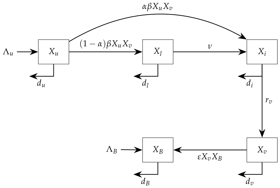
The schematic diagram (
Figure 1) illustrates the compartmental structure and interaction pathways of the model. It shows the five state variables—uninfected CD4
+ T cells (
), latently infected cells (
), actively infected cells (
), free virions (
), and B cells (
)—along with the infection routes
, delay stages
, and key processes such as latent cell activation
, viral production
, and B-cell stimulation
in response to free virions.
Therefore, the proposed model illustrates the coupled, delay-dependent structure of HIV pathogenesis, emphasizing the roles of latency, delayed viral replication, and the role of B cells in antiviral response. In particular, the mathematical model provides the following key elements:
Two routes of infection—latent () and active ()—with distributed delays ().
Latent cells () activate at rate to become active cells ()—with distributed delay ().
Active cells produce virions after intracellular delay .
The presence of HIV stimulates the proliferation of B cells at a rate .
For
, the functions
represent probability density functions for the distributed delays, defined on
with
possibly infinite, satisfying
We define , satisfying .
Based on the schematic diagram (
Figure 1), we consider the following system of delay differential equations that describes the within-host dynamics of HIV infection, taking into account latent reservoirs, distributed delays in infection and viral production, and the immune response mediated by B cells:
for all
.
For each delay process , a probability density function is introduced, defined on the interval with possibly infinite. These density functions satisfy and . To incorporate both the distribution of the time lag and the decay of infected cells or virions during the delay period, the effective kernel is defined as , where is a decay rate. The total contribution from all past times to a given compartment at time t is then represented by the integral , where Y denotes the relevant variable (e.g., for infection terms, or or for activation and production terms). This formulation generalizes discrete delays (obtained when is a Dirac delta function) and allows for more realistic distributions such as gamma or uniform delays. The net effect of each delay on the infection threshold is summarized by the factor , which satisfies and appears explicitly in the delay-dependent basic reproduction number .
The system (
1)–(
5) is equipped with initial values given by continuous functions on the delay interval
:
where
, and
. The equations describe the HIV dynamics on
with initial values given on
.
Assumption 1 (Model Assumption). The death rates satisfy: .
This inequality establishes a biologically motivated hierarchy for the natural turnover rates of the T-cell populations. In fact, healthy cells are the most stable, latently infected cells form a persistent reservoir, and actively infected cells are short-lived due to viral cytotoxicity and immune attack.
Biological Interpretation of Terms
: Constant recruitment rate of uninfected CD4+ T cells.
: Production rate of B cells.
: Infection rate for both latent and active infections.
: Proportion of infections that directly lead to active infection. The remainder leads to latent infection.
: Activation rate of latently infected cells.
: Number of virions produced per actively infected cell per unit time.
: Neutralization rate of virions by B cells.
: Rate of B-cell proliferation stimulated by free virions. This term reflects the activation and expansion of the B-cell population in response to viral antigen, which enhances the humoral immune response.
: Death rates of uninfected T cells, latently infected cells, actively infected cells, free virions, and B cells, respectively.
Delays account for time between infection and appearance of latently/actively infected cells , delay in latent cell reactivation , and intracellular delay in virion production .
A summary of the biological interpretation of all variables and parameters in the distributed-delay HIV model (
1)–(
5) is given in
Table 2.
Remark 1. and describe the time from viral entry into a target cell until the cell becomes either latently infected () or actively infected (). During this period, reverse transcription, integration, and transcriptional silencing (for latency) or activation (for active infection) occur. This is the establishment delay. reflects the time from when a latently infected cell receives an activation stimulus (e.g., antigen encounter, cytokine signaling) until it transitions to an actively infected cell that produces virions. This is the reactivation delay. Thus, and do not double-count latency; rather, latency is the state in between. A latently infected cell exists for a period (with mean residence time ) before reactivation, and the delay represents the intracellular signaling and transcriptional initiation steps after stimulation.
Having established the full distributed-delay model with latent reservoirs and B-cell response, we next turn to a foundational analysis of the system in the absence of delays. This simplification allows us to derive the basic reproduction number and establish global stability properties in a more tractable setting, which will serve as a crucial benchmark for the subsequent analysis of the delayed system.
3. Global Analysis of the HIV Model Without Distributed Delays
Analyzing the non-delayed system first allows us to isolate the intrinsic dynamics of HIV infection from the effects of time lags. The threshold behavior established here provides a baseline against which the impact of distributed delays can be quantified in
Section 4. This section presents an analysis of the within-host HIV dynamics model in the absence of distributed delays. By setting all delay terms to zero, system (
1)–(
5) reduces to a system of ordinary differential equations (ODEs) that captures the fundamental interactions between uninfected CD4
+ T cells, latently infected cells, actively infected cells, free virions, and B cells. The simplified model allows for a more tractable examination of the system’s qualitative behavior, including the existence and stability of equilibria. We begin by establishing basic properties such as non-negativity and boundedness of solutions, ensuring the biological well-posedness of the model. Subsequently, the basic reproduction number
is derived using the next-generation matrix method, serving as a critical threshold that dictates the persistence or clearance of the infection. The global asymptotic stability of the infection-free equilibrium is proven for
, while the existence and global stability of a unique endemic equilibrium are established for
. These analytical results provide a foundational understanding of the system’s long-term behavior, which will later be extended to the more complex case incorporating distributed delays.
The HIV model without distributed delays is given hereafter.
for all
with initial condition
. The equations describe the HIV dynamics on
with initial values given at
.
3.1. Basic Properties: Positivity, Boundedness, and Invariant Region
This subsection establishes the fundamental mathematical properties of the ODE system (
7)–(
11) that ensure its biological plausibility and analytical tractability. We first prove that all state variables, uninfected CD4
+ T cells
, latently infected cells
, actively infected cells
, free virions
, and B cells
remain non-negative for all time
given non-negative initial conditions. This positivity property is essential for the model to represent meaningful biological concentrations. Subsequently, we demonstrate that the solutions of the system are ultimately bounded. By constructing appropriate Lyapunov-like functions and differential inequalities, we derive explicit upper bounds for each compartment and identify a positively invariant region
in the non-negative orthant
. This region acts as a global attractor, meaning all trajectories eventually enter and remain within
. Establishing these basic properties, positivity, boundedness, and the existence of a compact invariant set, forms the necessary foundation for the equilibrium and stability analysis carried out in the subsequent subsections. Let
.
Lemma 1. Dynamics (7)–(11) admit a positively invariant attractor set given by Proof. We have
Thus
for all
when
. Now, let us show the boundedness of the model’s solution. We we define
as
Then, we get
Thus,
and hence,
, for any
.
The non-negativity of solutions implies that , , if . □
3.2. Threshold Quantification and Equilibrium Analysis: The Basic Reproduction Number and Steady States
This subsection focuses on determining the long-term outcomes of the within-host HIV infection as predicted by the ODE model (
7)–(
11). The central object of this analysis is the basic reproduction number, denoted
, which serves as a critical epidemiological threshold.
is derived using the next-generation matrix method [
33,
34], explicitly accounting for both direct infection pathways (via actively infected cells) and the indirect contribution from the latent reservoir. We analytically characterize all possible steady-state solutions (equilibria) of the system. The infection-free equilibrium
, representing the complete clearance of the virus, is shown to always exist. Furthermore, we establish that a unique endemic (chronic) equilibrium
, corresponding to a persistent infection state, exists if and only if
. The proof of existence and uniqueness relies on constructing an auxiliary function and applying monotonicity arguments. This threshold condition,
, precisely delineates the parameter regime where the virus can establish a sustained infection, thereby framing the subsequent stability analysis in
Section 3.3. Let us start by defining the matrices
and
as follows:
and
. Therefore, the spectral radius representing the basic reproduction number is the dominant eigenvalue, given by
Lemma 2. Dynamics (7)–(11) admits a trivial steady state denoted by . If then dynamics (7)–(11) admits an endemic steady state .
Proof. Steady states are obtained by setting all equations of dynamics (
7)–(
11) to zero:
We find that the given model (
7)–(
11) has two equilibria:
Infection-free equilibrium, .
Endemic equilibrium,
, where
where
, which satisfies the following equation:
, where
We define the quadratic function
as
. Since
,
is a strictly convex function on
. Furthermore, we have
Therefore,
if
as well as
. Since
is continuous on
, the intermediate value theorem ensures the existence of at least one
such that
. Since
, the function
is strictly convex, and therefore, it can have at most two real roots. Moreover, its derivative is
, which is strictly increasing on
.
Assume, for contradiction, that
admits two distinct positive roots
. Then, by Rolle’s theorem, there exists
such that
Since
is strictly increasing, it has exactly one zero, given by
. Thus,
decreases on
and increases on
.
Now, since and , the function must be strictly decreasing at least on an interval starting from 0, which implies . Therefore, is strictly decreasing on and strictly increasing on .
This implies that can cross the horizontal axis at most once in and at most once in . However, since and , the sign change occurs before reaching the minimum point . Hence, the root lies in the strictly decreasing region . Consequently, can admit only one root in the interval . Thus, there exists a unique such that satisfies . As a result, we get , , and .
□
3.3. Global Stability Analysis of Equilibria
This subsection establishes the global asymptotic stability properties of the equilibria identified in
Section 3.2, providing a complete qualitative picture of the system’s long-term dynamics for all possible initial conditions. We employ the method of Lyapunov functions, constructing suitable scalar energy-like functions for each equilibrium [
35]. First, for the case
, we prove that the infection-free equilibrium
is globally asymptotically stable (GAS). This result implies that regardless of the initial viral load, the infection will be cleared from the host if the basic reproduction number is at or below unity. Conversely, when
, we demonstrate that the unique endemic equilibrium
is GAS. This means the system will converge to the chronic infection state for any non-trivial initial condition, confirming the epidemiological threshold established earlier. The proofs leverage the classical LaSalle’s Invariance Principle and careful algebraic manipulations to show the negativity of the Lyapunov derivatives. These global stability results confirm the threshold dynamics governed solely by
, with no possibility of bistability or oscillatory persistence in the non-delayed model.
Define H as the nonnegative function that only vanishes at .
Theorem 1. The trivial equilibrium point is globally asymptotically stable once .
Proof. The proof is based on the Lyapunov function
given by
and uses LaSalle’s Invariance Principle [
36] to prove that
is GAS if
. More details are given in
Appendix A.1. □
Theorem 2. The endemic equilibrium is GAS when .
Proof. The proof is based on the Lyapunov function
given by
and by using LaSalle’s Invariance Principle [
36] to prove that
is GAS if
. More details are given in
Appendix A.2. □
In conclusion,
Section 3 has provided a complete analytical framework for the within-host HIV model in the absence of distributed delays. We established the model’s well-posedness by proving the positivity and ultimate boundedness of solutions, confining the dynamics to a biologically relevant invariant region
. The critical threshold for infection persistence was precisely quantified through the basic reproduction number
, derived via the next-generation matrix method. Our analysis demonstrated that the system exhibits a sharp threshold dynamic: when
, the infection-free equilibrium
is globally asymptotically stable, guaranteeing viral clearance, whereas when
, a unique endemic equilibrium
emerges and is globally asymptotically stable, leading to chronic infection. These results, proven using Lyapunov function techniques and LaSalle’s Invariance Principle, establish a solid foundation for understanding the basic interaction dynamics. The insights gained here form a crucial benchmark against which the more complex effects of distributed delays, analyzed in the subsequent section, can be evaluated.
4. Dynamics with Distributed Delays: Incorporating Realistic Time Lags
This section extends the analysis of the within-host HIV model by incorporating distributed time delays, which account for essential biological latencies in the infection process. The model (
1)–(
5) generalizes the ODE system (
7)–(
11) by introducing four distinct distributed delays:
and
for the time between viral entry and the emergence of latently and actively infected cells, respectively;
for the intracellular delay in virion production; and
for the delay in B-cell activation. These delays are modeled using general probability density functions
, making the framework adaptable to various delay distributions (e.g., discrete, gamma-distributed). We begin by establishing the fundamental properties of the delay system, including the non-negativity and ultimate boundedness of solutions, and identify a positively invariant attracting region. Subsequently, we derive the corresponding basic reproduction number
, which incorporates the delay kernels through integral factors
. We prove the existence of a unique endemic equilibrium when
. The core of this section is dedicated to proving the global asymptotic stability of both the infection-free equilibrium (for
) and the endemic equilibrium (for
), employing suitably constructed Lyapunov functionals that explicitly account for the distributed delays. This analysis reveals how time lags quantitatively alter the threshold condition and system dynamics while preserving the qualitative threshold behavior established in the non-delayed case.
4.1. Basic Properties of the Delay System
This subsection establishes the fundamental mathematical properties of the distributed-delay HIV model given by system (
1)–(
5). Ensuring the biological plausibility and analytical tractability of the model requires proving that its solutions remain nonnegative at all times—reflecting the physical reality of cell and virus concentrations—and that they are ultimately bounded within a biologically feasible region. We demonstrate the nonnegativity of solutions using a recursive argument based on the form of the equations and the nonnegative initial conditions specified in (
6). Subsequently, we prove the ultimate boundedness of all state variables by constructing appropriate auxiliary functions and deriving differential inequalities that yield explicit upper bounds. These bounds collectively define a compact, positively invariant set
in the nonnegative orthant
, which acts as a global attractor for the system’s trajectories. Establishing these basic properties—nonnegativity, boundedness, and the existence of an invariant region—forms the essential foundation for all subsequent equilibrium and stability analysis in the presence of distributed delays, guaranteeing that the model is well-posed and that its long-term dynamics are confined to a biologically meaningful domain.
Lemma 3. Solutions of model (1)–(5) with the initial states (6) are nonnegative and ultimately bounded. Furthermore, the setis positively invariant with respect to model (1)–(5). Proof. Let us show the nonnegativity of solutions of model (
1)–(
5). Clearly, Equations (
1) and (
5) of model (
1)–(
5) give
Hence,
and
for any
. In addition, we have
for any
. Hence, by recursive argumentation, we obtain
for any
.
Let us prove the ultimate boundedness of solution
. From Equation (
1), we have
. To prove the ultimate boundedness of
, we define
Then, we get
It follows that
and then
Define
Then, we get
It follows that
then
Now, let us define
Then, we obtain
where
. It follows that
and thus,
and
□
4.2. Equilibria and Thresholds
This subsection establishes the existence and uniqueness of equilibrium points for the distributed-delay HIV model (
1)–(
5) and derives the corresponding basic reproduction number
. The analysis proceeds by setting the time derivatives in system (
1)–(
5) to zero and solving the resulting algebraic equations. Two distinct steady states are identified: the infection-free equilibrium
, which always exists and represents the complete absence of the virus, and an endemic equilibrium
, which exists if and only if the basic reproduction number exceeds unity. The threshold
is derived via the next-generation matrix method [
34] applied to the linearized system at the infection-free state. Crucially,
incorporates the distributed-delay kernels through the integral factors
, which quantify the net effect of the time lags on viral transmission and progression. This generalized reproduction number reduces to the non-delay counterpart
when all delays vanish (
). The existence proof for the endemic equilibrium employs an auxiliary function and monotonicity arguments, demonstrating a unique biologically feasible chronic-infection state when
. These results extend the threshold analysis of
Section 3 to the more realistic setting with distributed delays, confirming that the qualitative threshold dynamics—characterized by a transcritical bifurcation at
—are preserved despite the incorporation of biological latencies [
37].
We proceed by calculating the delayed reproduction number
by deriving it from the linearization of the distributed-delay system around the disease-free equilibrium (DFE), and by showing how the delay kernels lead naturally to the appearance of the factors
[
34,
38].
From the model (
1)–(
5), the disease-free equilibrium is
Let us define the infected variables vector
The dynamics of
is obtained from (
2)–(
4). Linearizing around
(i.e., replacing
and
by their DFE values), we obtain
The above system is a linear system with distributed delays of convolution type. It can be written abstractly as
where
contains the
new infection terms (with delays), and
contains transition and removal terms.
Crucially, the delay terms represent the probability that an individual survives the delay period and contributes to infection at time
t. Indeed, each kernel has the form
so that
is the probability density that the transition occurs after a delay
with survival.
To compute the basic reproduction number, we consider exponential solutions of the form
. Substituting
, the delay integrals become Laplace transforms:
At the threshold (
), these reduce to
Thus, at the invasion threshold, each delayed transition contributes a factor , which represents the expected survival through the delay period.
Using the above reduction, the linearized system becomes equivalent (at threshold) to the following ODE system:
where
Here,
collects new infection terms,
describes transitions and removals (including delayed transitions weighted by ).
The delayed basic reproduction number is defined as the spectral radius of the next-generation matrix:
After explicit computation, this yields
Each factor arises rigorously from the Laplace transform of the delay kernel evaluated at and represents the probability that an individual:
Thus, the distributed-delay system induces a natural modification of the next-generation matrix, where each infection pathway is weighted by the corresponding survival probability through delays.
The Lemma 4 systematically analyzes the resulting algebraic system, distinguishing between the infection-free and endemic cases. We demonstrate that a unique endemic equilibrium emerges if and only if the delay-dependent reproduction number exceeds unity, mirroring the threshold behavior observed in the non-delayed case.
Lemma 4. Dynamics (1)–(5) admits an infection-free equilibrium . If , then dynamics (1)–(5) admits a unique endemic equilibrium .
Proof. Note that for an equilibrium, all time derivatives are zero and state variables are constant. Substituting constants
into the integral terms gives:
which holds because
(constant). Thus the equilibrium equations become algebraic and the factors
appear naturally.
The existence of equilibria for the distributed-delay system is established by solving the steady-state equations derived from setting the time derivatives in (
1)–(
5) to zero.
We find that the given model (
1)–(
5) admits two equilibria:
Infection-free equilibrium, .
An endemic equilibrium,
, where
where
satisfies the following equation:
where
Let us define a function
as
. Function
is continuous on
. Then, we have
and
. Similarly to the proof of Lemma 2,
if
as well as
. Since
G is continuous on
, the intermediate value theorem ensures the existence of at least one
such that
.
Since , the function G is strictly convex, and therefore it can have at most two real roots. Moreover, its derivative is , which is strictly increasing on .
Assume, for contradiction, that admits two distinct positive roots . Then, by Rolle’s theorem, there exists such that . Since is strictly increasing, it has exactly one zero, given by . Thus, G decreases on and increases on .
Now, since
and
, the function must be strictly decreasing at least on an interval starting from 0, which implies
. Therefore,
G is strictly decreasing on
and strictly increasing on
. This implies that
G can cross the horizontal axis at most once in
and at most once in
. However, since
the sign change occurs before reaching the minimum point
. Hence, the root lies in the strictly decreasing region
. Consequently,
G can admit only one root in the interval
. Thus, there exists a unique
such that
satisfies
. As a result, we get
,
,
and
. This provides the existence and uniqueness of the endemic equilibrium
once
.
□
4.3. Global Stability
This subsection is devoted to establishing the global asymptotic stability properties of the equilibria for the distributed-delay HIV model (
1)–(
5). We construct explicit Lyapunov functionals that incorporate integral terms to account for the distributed delays, thereby extending the Lyapunov function techniques [
32] used in the non-delayed case. For the infection-free equilibrium
, we prove that it is globally asymptotically stable (GAS) whenever
, implying that the infection will be cleared from the host regardless of the initial viral load if the basic reproduction number is at or below the critical threshold. Conversely, when
, we demonstrate that the unique endemic equilibrium
is GAS, ensuring convergence to a chronic infection state for all positive initial conditions. The proofs rely on the construction of carefully chosen Lyapunov functionals that include memory terms capturing the delay history, and the application of LaSalle’s Invariance Principle [
32] for delay systems. These results confirm that the qualitative threshold behavior—where the dynamics are governed solely by
—persists even in the presence of distributed delays, with no emergence of bistability or sustained oscillations. The analysis thus provides a foundation for understanding how biological latencies influence the long-term fate of the infection without altering the fundamental eradication-persistence dichotomy.
Let us define the number . Note that .
Theorem 3. The system (1)–(5) is globally asymptotically stable (GAS) around the infection-free equilibrium if . Proof. The proof is based on the Lyapunov function
given by
and by using the Lyapunov–LaSalle asymptotic stability theorem [
32] to prove that
is GAS if
. More details are given in
Appendix B.1. □
Theorem 4. The system (1)–(5) is GAS around the endemic equilibrium once . Proof. The proof is based on the Lyapunov function
given by
and by using the Lyapunov–LaSalle asymptotic stability theorem [
32] to prove that
is GAS if
. More details are given in
Appendix B.2. □
In conclusion,
Section 4 has successfully extended the analytical framework of the within-host HIV model to incorporate distributed time delays, reflecting essential biological latencies in infection and immune response processes. We established the well-posedness of the delay system by proving the non-negativity and ultimate boundedness of solutions, confining the dynamics to a biologically meaningful invariant region. The generalized basic reproduction number
was derived, explicitly incorporating delay kernels through integral factors
, and shown to govern a sharp threshold for infection persistence. Using carefully constructed Lyapunov functionals that account for the delay history, we proved the global asymptotic stability of the infection-free equilibrium when
and of the endemic equilibrium when
. These results demonstrate that although distributed delays quantitatively alter the threshold condition and system dynamics—by reducing
through the factors
—they do not change the fundamental qualitative behavior: the system still exhibits a transcritical bifurcation at
, with no introduction of bistability or persistent oscillations. This analysis provides a robust theoretical foundation for understanding the impact of biological time lags on HIV dynamics and sets the stage for the numerical exploration of sensitivity, treatment effects, and delay-induced critical thresholds in
Section 5.
5. Numerical Results and Discussion
This section presents a numerical investigation of the distributed-delay HIV model to illustrate the analytical results derived in previous sections and to explore the quantitative impact of key biological and pharmacological factors. We begin by specifying the delay structure, choosing the Dirac delta function
as a particular probability density, which reduces the general distributed-delay system to a discrete-delay model as the one given in [
28] with fixed delays
and survival probabilities
. Using a biologically plausible set of parameter values (
Table 3), we perform numerical simulations to validate the stability theorems: first, by selecting parameters such that
and demonstrating convergence to the infection-free equilibrium
; and second, by increasing infection rates to achieve
and showing convergence to the endemic equilibrium
. We then conduct a detailed sensitivity analysis of
, deriving and computing normalized sensitivity indices to rank parameters by their influence on the basic reproduction number. This analysis identifies the most effective targets for intervention. Furthermore, we examine the dynamics under antiretroviral treatment by incorporating an efficacy parameter
, deriving the treatment-dependent reproduction number
and determining the critical drug efficacy
required for viral eradication. Finally, we investigate the specific impact of the intracellular production delay
on the threshold condition, computing the critical delay
that suppresses the infection. Together, these numerical explorations bridge the theoretical analysis with practical insights, highlighting how delays, treatment, and parameter variations shape the within-host dynamics of HIV.
By choosing the Dirac delta function
as a specific form of the probability distribution, we define
. In case
, we get
, and
. Then,
Hence, model (
1)–(
5) can be written as
for all
where the initial values are picked as constants functions on
. For simplicity, in all numerical simulations, we choose the delay parameters as
.
The basic reproduction number of model (
12) is given by:
5.1. Validation of Global Stability
This subsection provides numerical validation of the global stability theorems established in
Section 3 and
Section 4 by simulating the dynamics of the discrete-delay HIV model given by system (
12). Using the baseline parameter values from
Table 3 with
, we select two distinct incidence rates (
) to illustrate the threshold behavior governed by the basic reproduction number
. Note that our aim is qualitative validation of analytical stability results, not quantitative clinical prediction; nonetheless, the parameters lie within physiologically plausible ranges.
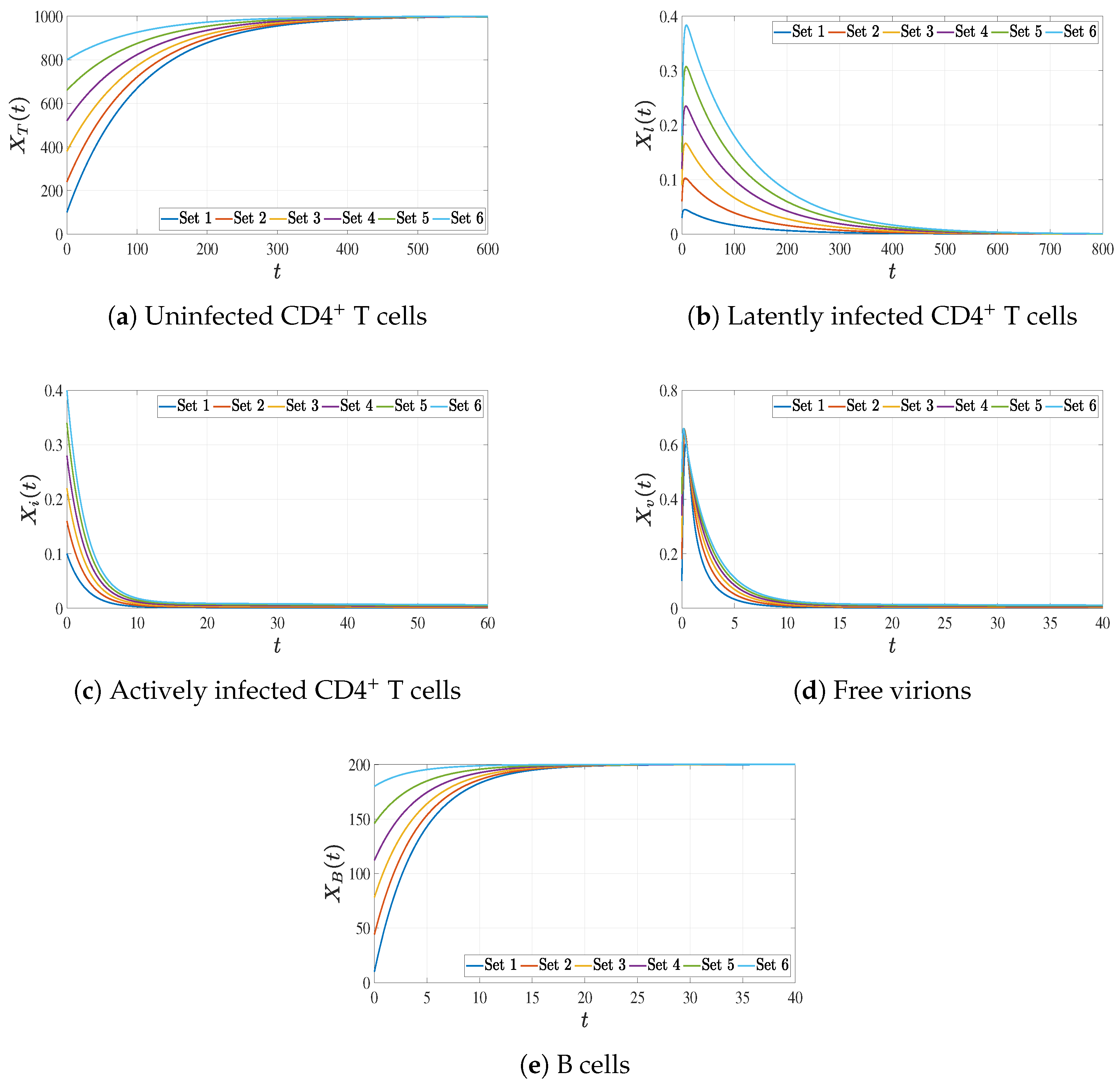
First, with infection rate
, we obtain
, confirming that the infection-free equilibrium
is globally asymptotically stable (GAS). Simulations of all compartment trajectories, uninfected CD4
+ T cells, latently infected cells, actively infected cells, free virions, and B cells demonstrate clear convergence to
, as shown in
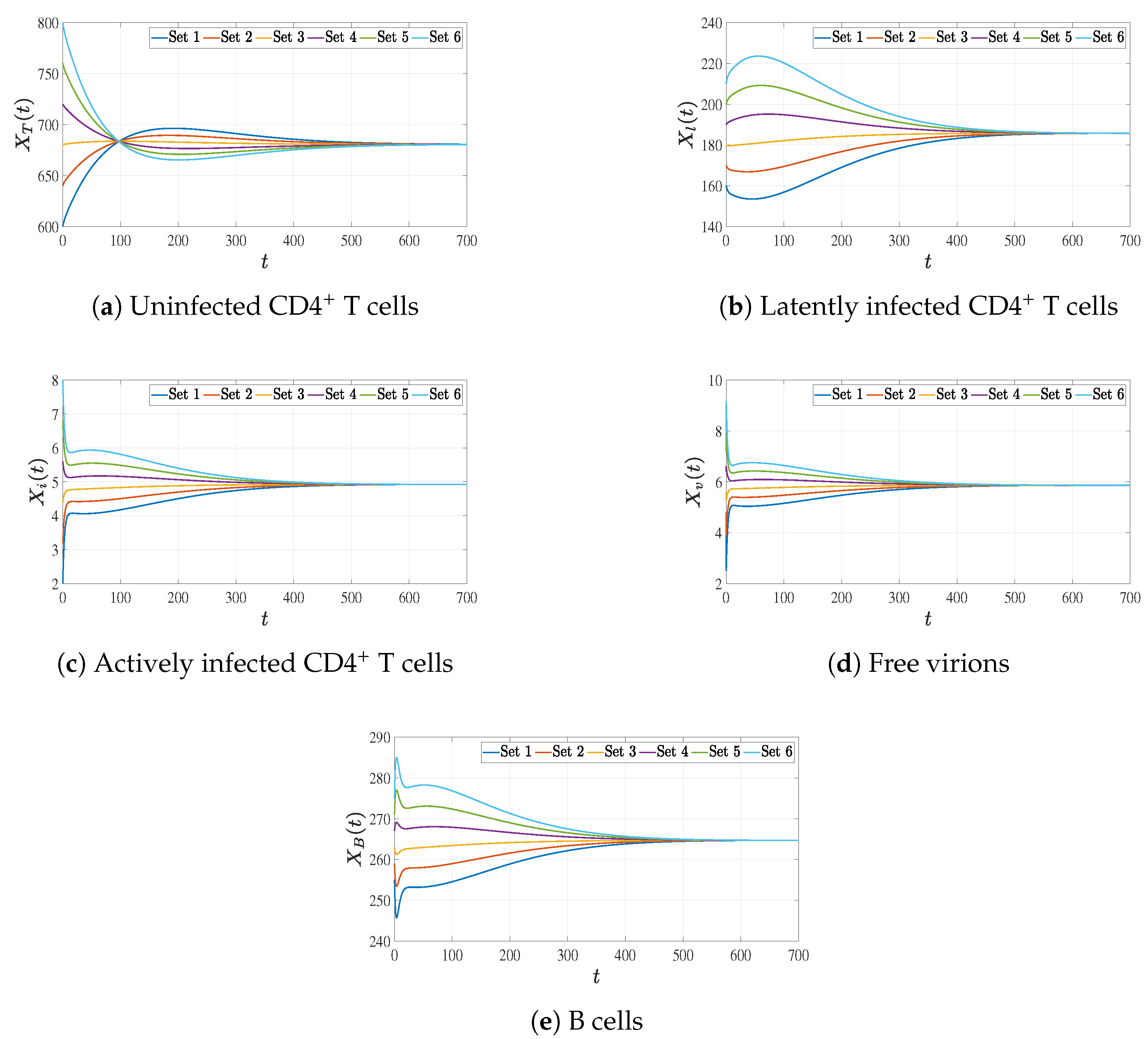
Figure 2. Second, by increasing the infection rate to
, we obtain
, which ensures the existence and global stability of the unique endemic equilibrium
. Corresponding simulations (
Figure 3) show convergence of all state variables to positive steady-state values, illustrating the establishment of a chronic infection. These numerical results not only corroborate the analytical stability proofs but also visually demonstrate the sharp threshold dynamics: the system transitions from viral clearance to persistent infection precisely as
crosses unity. The simulations were performed using standard delay differential equation solvers with biologically consistent initial conditions, further confirming the model’s robustness and the practical relevance of the theoretical threshold.
Figure 2 demonstrates convergence of all compartment trajectories to
. This confirms the theoretical result that when
, the infection is cleared and the system returns to a healthy state regardless of initial viral load.
Figure 3 shows trajectories converging to positive steady-state values, illustrating the establishment of a chronic infection. It validates the analytical prediction that a unique endemic equilibrium exists and is globally stable when
.
Figure 2.
Time series of the model variables for different constant history values (see
Table 2). Each color corresponds to one set of initial history values listed in
Table 4. For
, we get
, therefore,
is GAS.
Figure 2.
Time series of the model variables for different constant history values (see
Table 2). Each color corresponds to one set of initial history values listed in
Table 4. For
, we get
, therefore,
is GAS.
Figure 3.
Time series of the model variables for different constant history values (see
Table 3). Each color corresponds to one set of initial history values listed in
Table 5. For
, we get
; therefore,
is GAS.
Figure 3.
Time series of the model variables for different constant history values (see
Table 3). Each color corresponds to one set of initial history values listed in
Table 5. For
, we get
; therefore,
is GAS.
5.2. Sensitivity Analysis of
To quantify how variations in individual model parameters influence the basic reproduction number
, we perform a normalized forward sensitivity analysis [
48,
49]. The normalized sensitivity index (or elasticity) of
with respect to a parameter
p is defined as
.
The analytical expression for is , where the delay factors are given by . The partial derivatives of with respect to each parameter are computed, and the corresponding sensitivity indices are as follows:
Parameters appearing linearly in the numerator:
Parameters appearing linearly in the denominator:
Parameters in the activation term:
Parameters in the delay factors
:
Numerical Sensitivity Ranking
Using the baseline parameter values from
Table 3 with
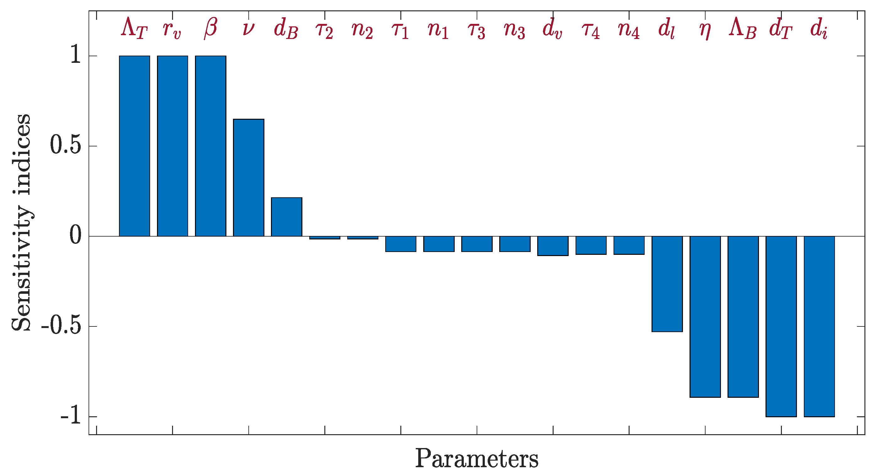
, the computed sensitivity indices are as shown below in
Figure 4 and
Table 6.
The bar chart in
Figure 4 displays normalized sensitivity indices (
) for each parameter, quantifying their relative influence on
. Positive values (e.g.,
,
,
,
) indicate that increasing the parameter raises
, while negative values (e.g.,
,
,
,
,
, delay-related parameters) signify a reducing effect. This visualization helps identify priority targets for intervention.
5.3. Treatment Effects
Drugs such as zidovudine (AZT), tenofovir, and emtricitabine inhibit the reverse transcription of viral RNA into DNA, thereby blocking new infections. In our model, this is represented by reducing the infection rate
by a factor
, where
represents drug efficacy:
Clinical studies by Deeks et al. [
50] report that RTIs typically achieve 70–90% inhibition of viral replication when used as monotherapy, and 90–95% when combined with other agents. The efficacy parameter
can be interpreted as the fraction of reverse transcription events that are successfully blocked.
The corresponding basic reproduction number under treatment,
, decreases linearly with increasing drug efficacy, directly linking pharmacological intervention to the infection threshold. We derive the critical drug efficacy
, which represents the minimum treatment effectiveness required to reduce
below unity and ensure viral eradication. Using numerical simulations, we explore how varying
influences the system’s long-term behavior.
Table 7 summarizes the values of
for different efficacies, illustrating the transition from endemic persistence (
) to infection clearance (
).
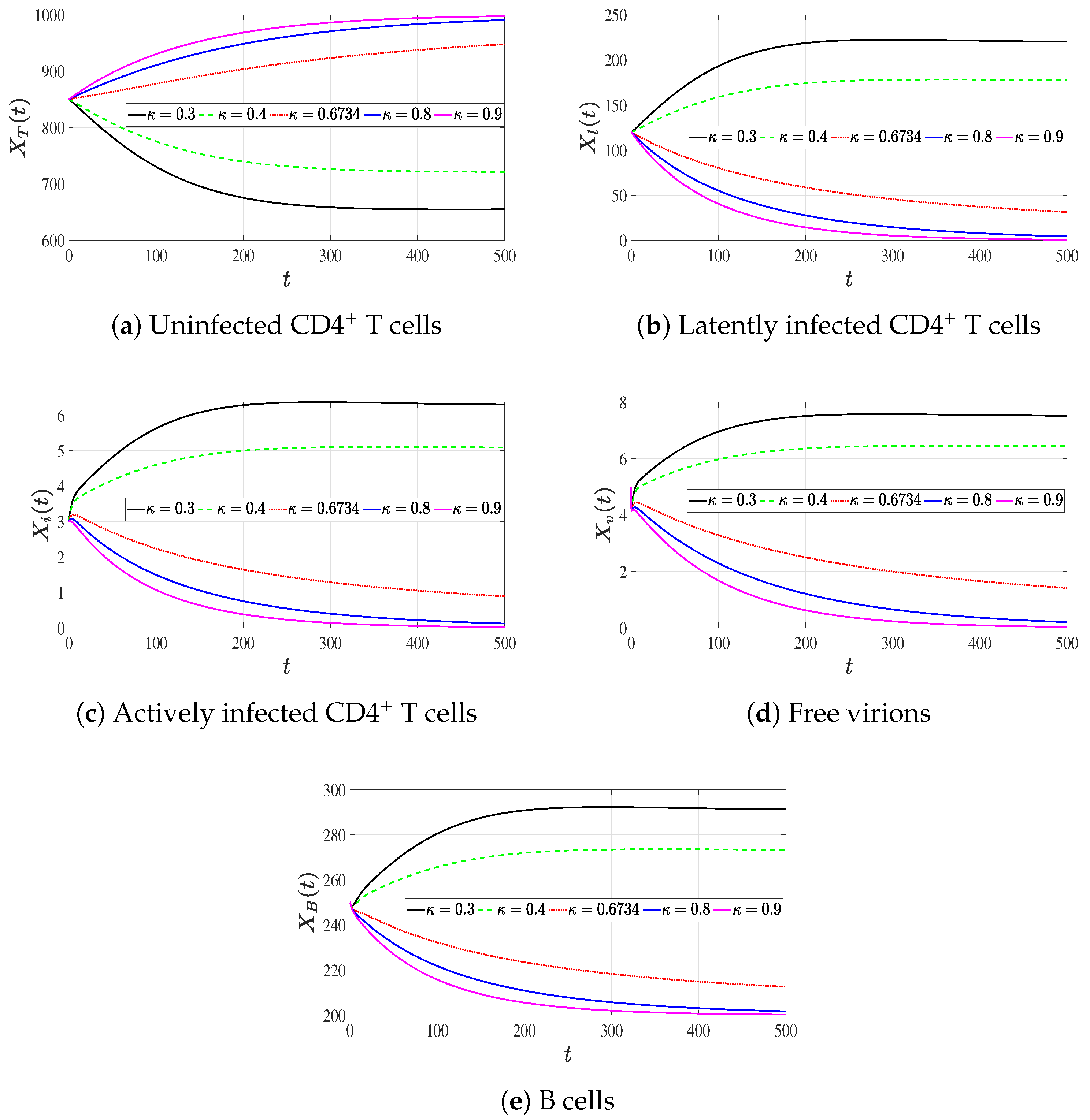
Figure 5 visually demonstrates this transition by plotting compartment trajectories for representative
values, showing how effective treatment suppresses viral load and enables immune recovery. These results highlight the critical role of treatment adherence and efficacy in achieving undetectable viral loads and provide a quantitative framework for assessing the necessary intervention intensity to shift the system from chronic infection to a disease-free state.
The model in the presence of treatment with an efficacy parameter
is given as follows:
for all
where the initial values are picked as constant functions on
.
The basic reproduction number in the presence of treatment can be expressed as follows: The critical drug efficacy necessary for viral eradication is obtained by solving the following inequalities: ensuring for all .
By using the baseline parameter values from
Table 3 and fixing the parameters
and
, and varying
, we study the impact of drug efficacy,
, on the stability of
. The approximated critical value of
is given by
. If
, then
, and the global stability of
. However, if
,
exceeds 1, destabilizing
.
The plots in
Figure 5 illustrate how varying levels of antiretroviral therapy affect viral load and immune cell populations. As
increases,
decreases, leading to suppression of the virus and eventual convergence to the infection-free state when
.
5.4. Delay Impact
This subsection examines the specific influence of the intracellular production delay
, representing the time between active infection and virion release, on the infection threshold and long-term dynamics. The basic reproduction number
depends exponentially on
via the factor
, making this delay a critical modulator of infection persistence. We derive an explicit expression for the critical delay
by solving
, yielding
If
, then
and the infection-free equilibrium is globally stable; conversely, if
, the endemic equilibrium prevails. Using baseline parameters, we compute
days.
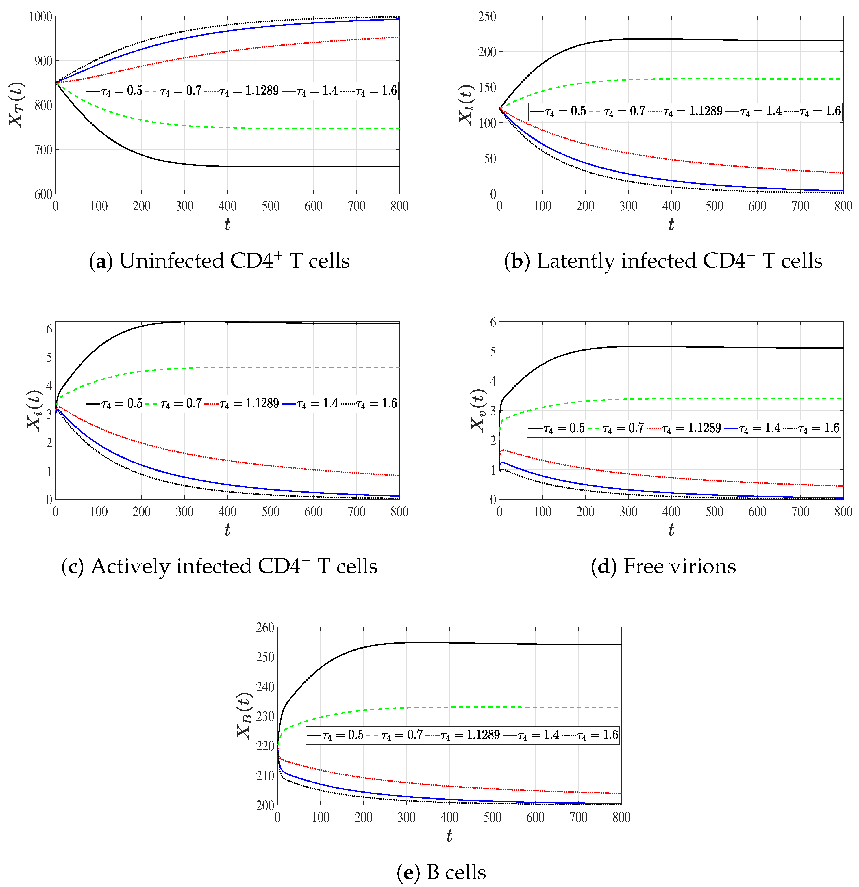
Figure 6 illustrates the effect of varying
on system trajectories, showing how increasing
progressively suppresses viral load and can eventually lead to infection clearance. This analysis underscores the potential role of delay-inducing therapeutic strategies, such as drugs that prolong the intracellular viral maturation phase, in pushing
below the critical threshold. It also highlights the sensitivity of the infection outcome to variations in this biological latency, providing insight into how natural or induced delays can fundamentally alter the course of HIV infection.
To guarantee that
, we compute the critical values
as
By using the baseline parameter values from
Table 3, fixing the parameters
and
, and varying
, we study the impact of the time delay,
, on the stability of
. The approximated critical value of
is given by
. If
, then
, and the global stability of
. However, if
,
exceeds 1, destabilizing
.
Figure 6 and
Table 8 show how increasing the intracellular production delay
reduces viral load and can shift the system from an endemic to an infection-free state when
. This highlights the potential therapeutic benefit of prolonging viral maturation.
6. Conclusions
This paper presented a mathematical analysis of a within-host HIV infection model incorporating latent reservoirs, distributed time delays, and a B-cell-mediated immune response. The model, formulated as a system of nonlinear delay differential equations, captures essential biological features: time lags between viral entry and infected cell emergence, latent cell reactivation, intracellular viral production, and B-cell proliferation in response to viral stimulation.
The study established well-posedness by proving non-negativity and boundedness of solutions, identifying a positively invariant region. For the non-delayed system, the basic reproduction number was derived, and a sharp threshold dynamic was proved using Lyapunov functions and LaSalle’s Invariance Principle: the infection-free equilibrium is globally asymptotically stable (GAS) when , while a unique endemic equilibrium is GAS when . These results were extended to the distributed-delay system, yielding a generalized reproduction number incorporating delay kernel integrals . The same threshold behavior persists: the infection-free equilibrium is GAS when , and the endemic equilibrium is GAS when , confirming that distributed delays quantitatively alter the threshold but do not introduce bistability or sustained oscillations.
Numerical simulations validated the analytical results. Sensitivity analysis identified the most influential parameters for intervention, including viral production rate , recruitment rates and , infection rate , neutralization rate , and death rates and . Treatment effects were explored, showing that drug efficacy linearly reduces , with critical efficacy derived for viral eradication. The intracellular delay was shown to act as a critical threshold, where increasing can suppress below unity, highlighting potential delay-inducing therapeutic strategies.
The model has several limitations: linear incidence terms (may not capture all virus–cell and immune nonlinearities); absence of spatial heterogeneity, drug resistance mutations, and CTL dynamics; the need for precise biological forms of delay kernels; and inter-patient variability affecting quantitative generalizability. The B-cell proliferation term assumes purely stimulatory effects without incorporating potential HIV-induced B-cell impairment or exhaustion, representing a baseline scenario for future extension once more detailed biological data become available.
Several future directions emerge: first, incorporating drug-specific mechanisms (reverse transcriptase inhibitors, protease inhibitors) and pharmacokinetics would improve representation of combination ART; second, extending the model to include CTL responses and viral mutation dynamics would allow study of immune escape and long-term treatment failure; third, connecting within-host to between-host transmission dynamics could bridge individual-level pathogenesis to population-level epidemiology; fourth, validating the model with longitudinal clinical data would enable patient-specific parameter estimation; fifth, exploring optimal control strategies based on sensitivity analysis could inform personalized treatment schedules, minimizing viral load while limiting toxicity and resistance; sixth, determining whether the global stability results extend to saturated (Holling type II) or other nonlinear incidence functions—numerical simulations suggest persistence of threshold behavior, but rigorous Lyapunov construction is non-trivial. Seventh, the distributed-delay formulation connects naturally to survival analysis frameworks: delay kernels
can be interpreted as survival-weighted probability densities, and factors
correspond to cumulative survival probabilities. This opens the door to estimating delay parameters from clinical survival data using inverse Gaussian or other parametric survival models [
51,
52], with future work combining survival analysis with DDEs. Eighth, while the present analysis proves global stability for positive kernels, bifurcation phenomena may arise under alternative assumptions; a systematic bifurcation analysis is deferred to future work, investigating saturated incidence, gamma-distributed delays, oscillatory kernels, and numerical bifurcation continuation to map stability regions and possible periodic solutions.
In summary, this work provides a mathematical framework for understanding the roles of latency, distributed delays, and immune response in HIV dynamics, underscoring threshold-based approaches for predicting infection outcomes and identifying therapeutic avenues.