Optimization of a Hybrid EKF-ANN Model via Double-Criterion Early Stop Pruning for Enhanced Wind Speed Forecasting

Abstract

A novel double-criterion early stopping pruning strategy is introduced in this study. The proposed approach enables the structural optimization of a hybrid filtering framework that integrates FeedForward Neural Networks with an adaptive Extended Kalman Filter, by simultaneously monitoring the validation error and the trace of the error covariance matrix. Unlike classical pruning methods, which are applied after the completion of the training process and aggressively remove network neurons, the proposed scheme exploits the learning procedure, achieving a more selective reduction of 2% to 13%, balancing effectively between strong generalization performance and computationally efficient training. The proposed framework is evaluated on wind speed forecasts obtained from a numerical weather prediction model, within a time-varying window scheme, demonstrating promising improvements. Key statistical indices, such as the Mean Absolute Error and the Root Mean Square Error, were significantly reduced, with reductions ranging from approximately 65% to 80% and 60% to 78%, respectively. These findings suggest that the proposed methodology offers a robust and accurate framework for time series forecasting in operational settings.

1. Introduction

Accurate forecasting of time series generated by stochastic dynamical systems remains a challenging problem in applied mathematics, particularly in the presence of uncertainty and model imperfections. In many real-world applications, the underlying processes are governed by complex, nonlinear dynamics, rendering purely deterministic or purely data-driven approaches insufficient for achieving reliable predictions. As a result, methodologies that utilize heavy statistical estimation techniques or advanced machine learning models have attracted increasing attention.

Kariniotakis and Pinson [1] demonstrated the effectiveness of fuzzy logic models in managing the inherent uncertainty of wind power data, while Kariniotakis et al. [2] established that the performance of such predictive models is heavily influenced by site-specific environmental characteristics. The importance of long-term stochastic modeling in capturing the variability of extreme physical phenomena was further explored by Vanem [3], providing a rigorous framework for time-dependent environmental variables. From a systemic perspective, Giebel [4] emphasized the benefits of understanding distributed power generation in mitigating the variability of stochastic energy sources. Furthermore, the mathematical foundations of risk and uncertainty in such complex systems were addressed by Resconi [5] through the geometry of morphogenetic systems.

Recent advances in time-series forecasting highlight the effectiveness of hybrid and error-correction-based approaches. Chang et al. [6] proposed a hybrid framework combining subsequence correction with multi-scale deep learning regression for long-term wind power forecasting, demonstrating improved performance in stochastic energy systems. Similarly, Aminjan et al. [7] addressed non-stationary and multi-regime dynamics in complex physical processes such as gas–liquid two-phase flows, where deep learning models are used to capture regime transitions and abrupt changes in system behavior.

Motivated by these requirements, hybrid estimation frameworks that integrate state-space modeling with neural network-based function approximation offer a promising direction for robust forecasting under uncertainty. Donas et al. [8] introduced such a hybrid framework that effectively enhances numerical weather and wave prediction models by dynamically adjusting to non-linear error patterns through parametrized ANNs. Within this context, the Hybrid Extended Kalman Filter (HEKF), which combines FeedForward Neural Networks (FFNNs) with an adaptive Extended Kalman Filter (EKF), has been successfully employed to produce accurate time series forecasts, reducing both systematic and non-systematic components of forecast error.

In this framework, an FFNN is first utilized to estimate an exogenous parameter (parametrized FeedForward Neural Network-pFFNN) governing the evolution of the EKF covariance matrices. Afterwards, based on the estimated parameter, the EKF is applied as a sequential training algorithm for a second FFNN, which generates the final improved predictions. This two-stage structure ensures both adaptability and computational efficiency, making the framework suitable for practical implementations.

Despite its effectiveness, the HEKF scheme presents a notable limitation, since the phenomenon of overfitting is poorly addressed, specifically in its second stage. Overfitting occurs when a model learns the training data too closely, resulting in reduced generalization performance on unseen data. Consequently, as Jabbar and Khan [9] note, controlling model complexity through robust strategies is crucial for maintaining predictive reliability in supervised learning tasks and for mitigating overfitting. Therefore, the present study extends the original HEKF formulation by introducing a novel double-criterion early stopping and pruning strategy to enhance its predictive performance.

More precisely, the proposed approach integrates validation-driven learning with a covariance-informed structural pruning mechanism, enabling the simultaneous control of model complexity and estimation uncertainty. Specifically, the training process is guided by the joint minimization of the validation error and the trace of the error covariance matrix. In addition, pruning decisions are based on the asymptotic properties of the error covariance matrix, allowing the removal of entire connection paths with negligible contribution. The novelty of the suggested modification lies in embedding the pruning mechanism within the sequential learning dynamics of the EKF, in contrast to classical pruning approaches that are applied after the training procedure. This formulation provides a statistically consistent framework for mitigating overfitting in hybrid filtering systems.

The effectiveness of the proposed mechanism is evaluated through its application to wind speed forecasts derived from the Weather Research and Forecasting (WRF) numerical weather prediction model with the Advanced Research dynamic core. More thoroughly, the analysis is conducted within a time-window framework, allowing for sequential training and evaluation. The suggested hybrid scheme is compared against the baseline HEKF, classical pruning techniques, and the raw WRF outputs, in terms of forecasting accuracy and computational efficiency.

In summary, the novelty and key contributions of the proposed study are as follows:

• Novel Double-Criterion Strategy: Introduction of a data-driven early stopping pruning mechanism that monitors both the validation error and the trace of the error covariance matrix simultaneously.
• Dynamic Structural Optimization: Pruning occurs dynamically during the EKF learning process, ensuring real-time model refinement rather than post-training adjustment.
• Selective Complexity Reduction: Achieves a balanced network by removing only 2–13% of redundant neurons, preserving essential non-linear mapping capabilities.
• Performance and Efficiency: Significant reduction in errors (up to 80% in MAE) combined with a 50% decrease in computational training time.

2. Methodology

The proposed hybrid framework is introduced in this section. Specifically, Section 2.1 presents the overall architecture, while Section 2.2 presents the core components of the HEKF. Section 2.3 introduces the proposed double-criterion pruning methodology, whereas Section 2.4 outlines the WRF time-window experimental design.

2.1. Hybrid Framework Overview

The original HEKF is structured into two main stages: (i) a selection stage, in which a FeedForward Neural Network is trained across different configurations of hidden neurons and memory parameter values to define the optimal combination, and (ii) an adaptive Extended Kalman Filter stage, acting as a training algorithm for a second FeedForward Neural Network, which produces the improved forecasts for the wind speed.

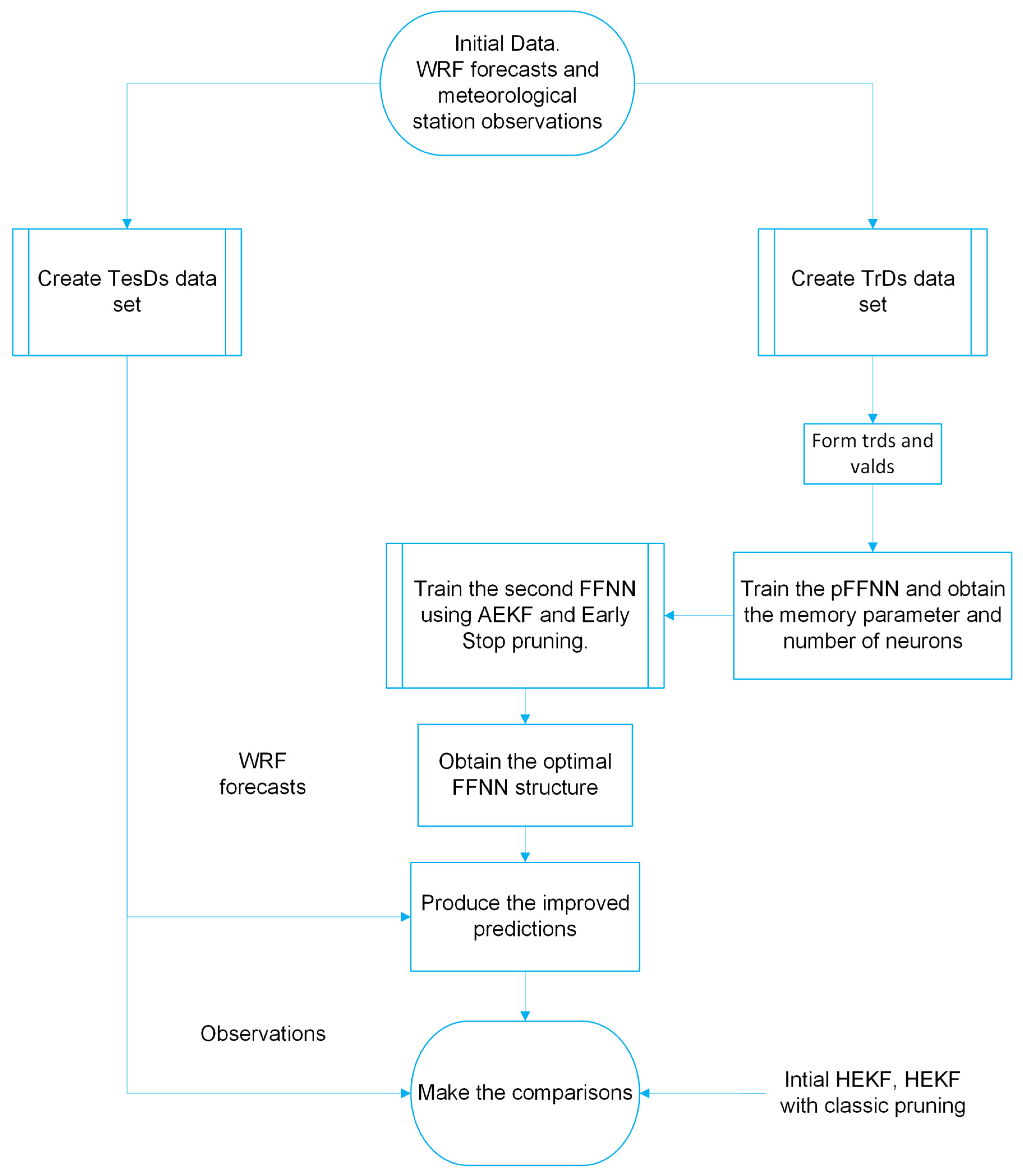
Initially, the available data, consisting of WRF forecasts and corresponding (recorded) observations, were partitioned into two subsets: the Training Dataset (TrDs) and the Testing Dataset (TesDs). The TrDs dataset trains the pFFNN and identifies the optimal combination, acting as a parameter estimation mechanism. To achieve this, the TrDs was further divided into the training data set (trds) and the validation data set (valds), where the former was employed to update the network weights, and the latter was used to monitor its (validation) error and determine the stopping point of the training process. That concludes the first stage of the initial HEKF approach.

Subsequently, the adaptive EKF framework was employed to train a distinct feedforward network, utilizing the optimal configuration obtained from the parametrized FFNN. More specifically, the chosen memory parameter updates dynamically the state and measurement covariance matrices during the EKF algorithm, while the selected number of hidden neurons determines the size of the second FeedForward Neural Network.

At this point of the second stage, the proposed expansion was introduced. In contrast to the baseline HEKF, which processes the TrDs in a single pass to estimate the optimal weights, the proposed framework suggests an iterative strategy. Particularly, the already defined training and validation subsets (trds and valds) were exploited over multiple passes, simulating the epochs of a conventional artificial neural network training process. During each epoch, the weights that minimize the (validation) error and also produce the lowest trace of the error covariance matrix were retained. Here, an epoch is defined as a complete pass through the entire training dataset (trds), during which all input–output pairs were sequentially processed.

Based on this dual-criterion selection, the pruning process was carried out by evaluating the contribution of each connectivity path to the network’s performance. The importance of each path was quantified using second-order information from the EKF error covariance matrix, capturing the influence of each path on the network’s predictive accuracy as measured on the validation dataset. If the aggregated contribution of a given path fell below a predefined threshold, the entire connection associated with the corresponding neuron was pruned.

The reduced network, along with the corresponding weights and the error covariance matrix, was used to initialize the subsequent epoch. In this way, the training of the second FFNN was no longer based on a single-pass estimation, but on a validation-driven strategy that boosts its generalization capability and effectively mitigates overfitting effects. If the error was not reduced for several epochs, particularly ten, the training process was terminated, using the weights that satisfy the double-criterion check. Thus, an Early Stop pruning was established for the adaptive Extended Kalman Filter.

Once the training process of this hybrid filter was completed, the optimized (second) network architecture, using the TesDs dataset, was employed to generate improved forecasts for the environmental parameter under study. These were compared, in terms of predictive accuracy and computational efficiency, with those derived from the initial methodology and the classical pruning EKF technique, in which the pruning process was performed after training completion based on the final error covariance matrix.

Overall, the proposed framework consists of two sequential stages involving two distinct neural networks. The first network was employed to determine the optimal architecture and memory parameter, while the second network was trained using the EKF, incorporating the information derived from the first stage. This separation ensures a clear distinction between structural optimization and adaptive learning. More precisely, in the first stage, an FFNN was trained by minimizing the Mean Squared Error, which constitutes the objective function of this stage. In the second stage, the training process of a different FFNN was formulated as a recursive minimization of the forecast error, defined as the difference between observed values and model forecasts, which defines the objective function of the second stage. Therefore, each stage of the proposed hybrid framework was associated with a distinct objective function, operating in a complementary and sequential manner.

The key components of the proposed hybrid modification are illustrated in Figure 1.

2.2. Baseline HEKF Formulation

This sub-section presents the baseline Hybrid Extended Kalman Filter, highlighting its core components: (i) the parametrized FeedForward Neural Network and (ii) the adaptive Extended Kalman Filter.

2.2.1. Parametrized FeedForward Neural Networks

Artificial Neural Networks [10,11] are supervised machine learning mechanisms inspired by the functions of the human brain, aiming to unlock complex, non-linear relationships between independent input variables and their corresponding target outputs. ANNs are composed of interconnected processing units, named neurons, that communicate through weighted connections. Each neuron receives inputs and applies an activation function to generate a corresponding output, enabling information to propagate throughout the entire network. Therefore, a wide range of ANN architectures can be constructed [12].

This study, however, focuses on FeedForward Neural Networks [13]. FFNNs establish a mapping between input data and output responses through a unidirectional flow of information. They generally consist of multiple fully connected layers organized in a directed acyclic topology. Here, a fully connected, three-layer FFNN structure was employed, including a single hidden layer. According to the universal approximation theorem, it is sufficient to approximate nonlinear mappings with arbitrary accuracy. Furthermore, as an activation function, the suggested architecture utilizes the log-sigmoid [14,15,16]:

$$\phi (x)={\displaystyle \frac{1}{1+e^{-x}}}.$$

(1)

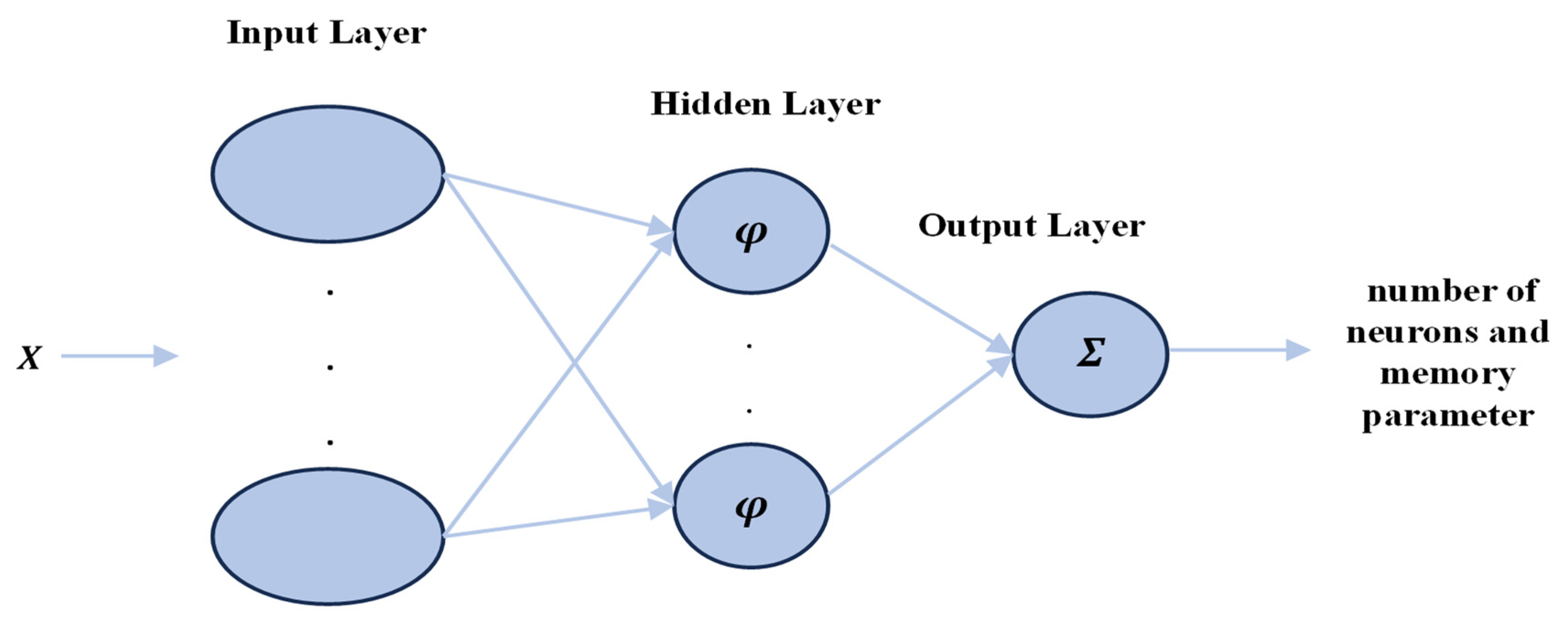
The proposed network was not designed to operate as a baseline forecasting tool, but rather as an estimation mechanism that determines the optimal combination of the number of hidden neurons and the value of a memory parameter, forming the so-called parametrized FeedForward Neural Network. To this end, the proposed network (Figure 2) utilizes an input matrix defined as:

$$X=(X_1,\dots ,X_t,\dots ,X_N,),$$

where $N$ presents the size of the TrDs, and $X_t$ represents the input vector at time $t$, consisting of two components: the WRF forecast (${for}_t$) and the memory parameter $\left(a\right)$; i.e.,

$$X_t={[{for}_t,a]}^T.$$

Based on this formulation, the pFFNN was trained for multiple values of the parameter $a$, aiming to identify the one that best captures the relationship between the input vectors and the corresponding targets, and for multiple numbers of hidden neurons. The parameter was selected within the range $[0.3, 0.4]$, while the number of neurons varies between 20 and 30. The structure that minimizes the Mean Squared Error (MSE) was considered optimal:

$$MSE={\displaystyle \frac{1}{N}}{\displaystyle {\sum }_{t=1}^N}{{(er}^t)}^2,$$

(2)

where ${er}^t=(T_t-X_t)$ denotes the training error between the scalar target $T_t$ and the corresponding input vector $X_t$.

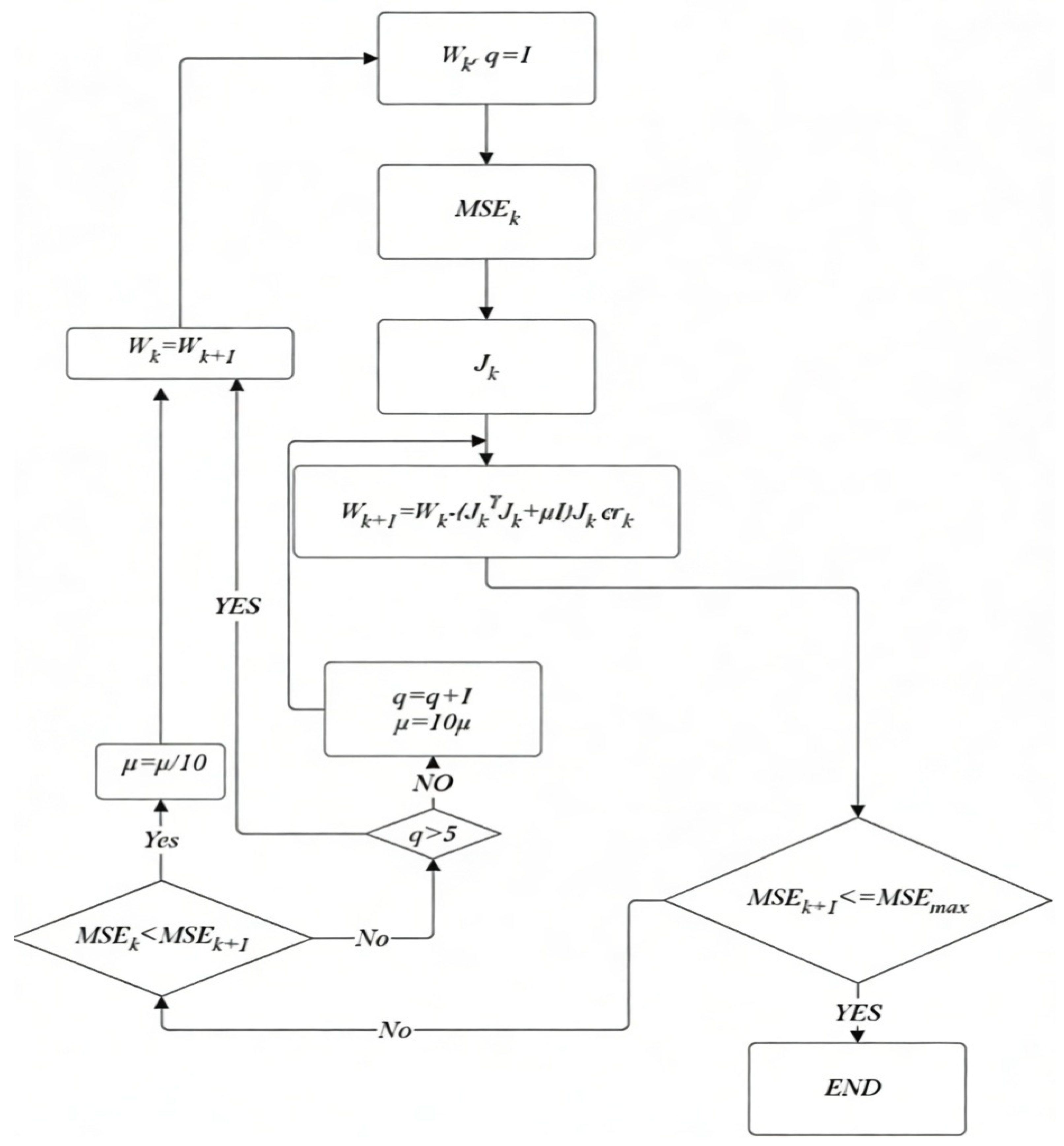
To minimize the MSE, an appropriate optimization procedure must be employed. Specifically, the Levenberg–Marquardt (LM) method was adopted in this study for training the pFFNN, due to its efficiency in problems involving a small number of the network’s weights and also because the MSE is used as a performance index [17]. The Levenberg–Marquardt algorithm integrates the principles of the steepest descent and Gauss–Newton methods to iteratively adjust the network weights during training. More specifically, at iteration $k$, the weight update is defined as follows [18]:

$$W_{k+1}=W_k-(J_k^T{J}_k+\mu {\rm I})J_k{er}_k,$$

(3)

where

• $W_k$ is a column vector consisting of the network’s variables (weights and biases).
• $J_k$ is the Jacobian matrix.
• ${er}_k$ represents the vectorized training error, i.e., ${er}_k={[{er}_k^1,\dots ,{er}_k^t,\dots {er}_k^N]}^T$.
• The quantity $(J_k^T{J}_k+\mu {\rm I})$ denotes an approximation of the Hessian matrix introduced by the LM algorithm, i.e., $Hes=(J_k^T{J}_k+\mu {\rm I})$.
• ${\rm I}$ is the identity matrix.
• $\mu$ is a combination parameter that takes positive values, ensuring the reversibility of the $J_k^T{J}_k$ matrix.

The computation of the Jacobian matrix constitutes a key step in the implementation of the LM algorithm, since it can be computationally intensive depending on the complexity of the network structure (number of neurons and hidden layers). In the case of the proposed parametrized FFNN, the Jacobian matrix is expressed as follows:

$$J_k={\displaystyle \frac{2}{N}}\left(\begin{array}{c}\begin{array}{cccccccccccc}{\displaystyle \frac{\mathsf{\partial }{er}_k^1}{\mathsf{\partial }{d}_{1,1}}}& {\displaystyle \frac{\mathsf{\partial }{er}_k^1}{\mathsf{\partial }{d}_{2,1}}}& \dots & {\displaystyle \frac{\mathsf{\partial }{er}_k^1}{\mathsf{\partial }{d}_{1,M}}}& {\displaystyle \frac{\mathsf{\partial }{er}_k^1}{\mathsf{\partial }{d}_{2,{\rm M}}}}& {\displaystyle \frac{\mathsf{\partial }{er}_k^1}{\mathsf{\partial }{b}_1}}& \dots & {\displaystyle \frac{\mathsf{\partial }{er}_k^1}{\mathsf{\partial }{b}_M}}& {\displaystyle \frac{\mathsf{\partial }{er}_k^1}{\mathsf{\partial }{v}_1}}& \dots & {\displaystyle \frac{\mathsf{\partial }{er}_k^1}{\mathsf{\partial }{v}_M}}& {\displaystyle \frac{\mathsf{\partial }{er}_k^1}{\mathsf{\partial }{b}_{out}}}\\ ⋮& ⋮& ⋮& ⋮& ⋮& ⋮& ⋮& ⋮& ⋮& ⋮& ⋮& ⋮\\ {\displaystyle \frac{\mathsf{\partial }{er}_k^t}{\mathsf{\partial }{d}_{1,1}}}& {\displaystyle \frac{\mathsf{\partial }{er}_k^t}{\mathsf{\partial }{d}_{2,1}}}& \dots & {\displaystyle \frac{\mathsf{\partial }{er}_k^t}{\mathsf{\partial }{d}_{1,M}}}& {\displaystyle \frac{\mathsf{\partial }{er}_k^t}{\mathsf{\partial }{d}_{2,{\rm M}}}}& {\displaystyle \frac{\mathsf{\partial }{er}_k^t}{\mathsf{\partial }{b}_1}}& \dots & {\displaystyle \frac{\mathsf{\partial }{er}_k^t}{\mathsf{\partial }{b}_M}}& {\displaystyle \frac{\mathsf{\partial }{er}_k^t}{\mathsf{\partial }{v}_1}}& \dots & {\displaystyle \frac{\mathsf{\partial }{er}_k^t}{\mathsf{\partial }{v}_M}}& {\displaystyle \frac{\mathsf{\partial }{er}_k^t}{\mathsf{\partial }{b}_{out}}}\\ ⋮& ⋮& ⋮& ⋮& ⋮& ⋮& ⋮& ⋮& ⋮& ⋮& ⋮& ⋮\\ {\displaystyle \frac{\mathsf{\partial }{er}_k^N}{\mathsf{\partial }{d}_{1,1}}}& {\displaystyle \frac{\mathsf{\partial }{er}_k^N}{\mathsf{\partial }{d}_{2,1}}}& \dots & {\displaystyle \frac{\mathsf{\partial }{er}_k^N}{\mathsf{\partial }{d}_{1,M}}}& {\displaystyle \frac{\mathsf{\partial }{er}_k^N}{\mathsf{\partial }{d}_{2,{\rm M}}}}& {\displaystyle \frac{\mathsf{\partial }{er}_k^N}{\mathsf{\partial }{b}_1}}& \dots & {\displaystyle \frac{\mathsf{\partial }{er}_k^N}{\mathsf{\partial }{b}_M}}& {\displaystyle \frac{\mathsf{\partial }{er}_k^N}{\mathsf{\partial }{v}_1}}& \dots & {\displaystyle \frac{\mathsf{\partial }{er}_k^N}{\mathsf{\partial }{v}_M}}& {\displaystyle \frac{\mathsf{\partial }{er}_k^N}{\mathsf{\partial }{b}_{out}}}\end{array}\end{array}\right)$$

wherein this case, we have the following:

• $d_{s,l}$ express the synaptic weight between the $s$ input and the $l$ neuron in the hidden layer. Here, $s=1,2$ and $l=1,\dots ,M$.
• $b_l$ and $v_l$ are the biases of the $l$ neuron and the corresponding synaptic weight between this neuron and the output layer, respectively.
• ${\displaystyle \frac{\mathsf{\partial }{er}_k^t}{\mathsf{\partial }{d}_{s,l}}}=-v_l\phi \prime ({net}_t^l)X_t^s$ and ${\displaystyle \frac{\mathsf{\partial }{er}_k^t}{\mathsf{\partial }{b}_l}}=v_1\phi \prime ({net}_t^l)$, with ${net}_t^l$ being the input of the $l$ neuron based on the $t$ training pattern, i.e., ${net}_t^l={\displaystyle {\sum }_{s=1}^2}{d}_{s,l}{X}_t^s+b_l$, where $X_t^s$ is the $s$ input of the $X_t$ input vector.
• ${\displaystyle \frac{\mathsf{\partial }{er}_k^t}{\mathsf{\partial }{v}_l}}={-v}_l\phi ({net}_t^l)$ and ${\displaystyle \frac{\mathsf{\partial }{er}_k^t}{\mathsf{\partial }{b}_{out}}}=-1$, where $b_{out}$ is the bias of the output layer.

Once the Jacobian matrix is computed, the training process of the suggested pFFNN based on the LM algorithm is illustrated in Figure 3.

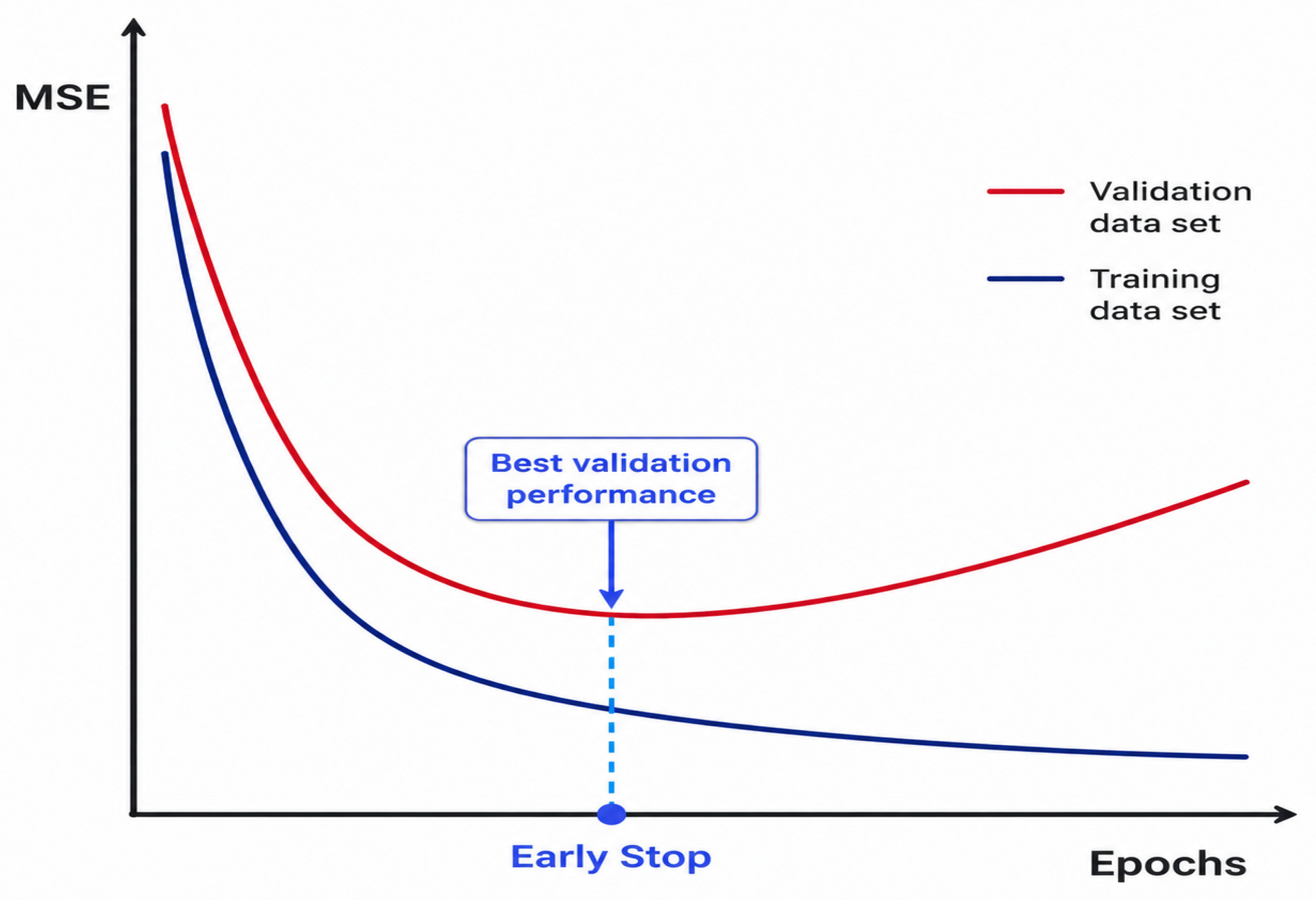
Apart from the training algorithm, another issue that emerges when dealing with ANNs is the phenomenon of overfitting [9]. To mitigate this malfunction and improve the network’s generalization, an early stopping strategy is employed [19]. During training, the network weights are updated using the training dataset at each epoch, while its performance is simultaneously evaluated on a validation dataset. If the validation error increases for several epochs, the training process is terminated, and the set of weights corresponding to the minimum validation error is selected as optimal (Figure 4). Properly handling overfitting is crucial for the successful implementation of the pFFNN.

Summarizing the above process,

Table 1. Basic elements of the parametrized FeedForward Neural Network.

ANN	FeedForward Neural Network
Neurons	20 to 30
Activation Function	Log-Sigmoid
Hidden Layers	1
Output Layer	One Linear Output
Memory Parameter $a$	0.3:0.01:0.4
Training Algorithm	Levenberg–Marquardt, $\mu =0.01$
Overfitting	Early Stop

presents the main characteristics of the proposed parametrized network, while in Appendix A, a detailed analysis of the first stage of the Hybrid Extended Kalman Filter is provided.

2.2.2. Adaptive Extended Kalman Filter

Once the training process of the pFFNN was finalized, the optimal combination of neurons and parameter $a$ was utilized in the following way: (i) the number of neurons determines the size of a second, three-layer, and fully connected FeedForward Neural Network, comprising a single hidden layer with a log-sigmoid activation function, that is trained using the Extended Kalman Filter [20,21], whereas (ii) the memory parameter was applied to update the state and the measurement covariance matrices during the EKF algorithm.

The selected network structure was consistent with the first stage of the proposed hybrid filter and also with the EKF-based training framework, as deeper architectures would significantly increase the dimensionality of the state vector and the associated computational cost of the covariance matrix updates. Therefore, an adaptive Extended Kalman Filter was created and employed as a learning rule, intending to determine the network’s optimal parameters.

Similar modified EKF algorithms have been frequently utilized as neural network training methods [22,23,24,25] due to their fast and efficient implementation [26]. These approaches are closely connected to sequential versions of the Gauss–Newton algorithm, and unlike the comparable batch variant, they do not require inversion of the approximate Hessian matrix [17].

To illustrate the training procedure of the adaptive EKF, a state-measurement model must be defined (Equations (4) and (5)). In this study, the corresponding model is formulated as:

$$W_t=W_{t-1}+w_{t-1}$$

(4)

$$y_t=f_t(W_t,{for}_t)+v_t,$$

(5)

where $W_t$ is a column vector that concludes the total weights of the FFNN at time $t$. The quantity $y_t$ presents the forecast error, defined as the difference between the recorded observation and the corresponding WRF forecast, at the same time. The variables $w_{t-1}$ and $v_t$ denote the Gaussian nonsystematic parts of the model error, with covariance matrices $Q_{t-1}$ and $R_t$, respectively. These are the state and measurement covariance matrices. Finally, $f(•)$ expresses the direct output of the second FFNN.

The proposed formulation assumes Gaussian noise characteristics, which is a standard assumption in Kalman filtering as it facilitates tractable probabilistic modeling and optimal state estimation under uncertainty [8,20,21]. Furthermore, the nonlinearity of the second FFNN, introduced by the $f(•)$ function, was addressed through local linearization of the measurement equation via a first-order Taylor expansion, as reflected in the computation of the Jacobian matrix required by the EKF.

When the state-measurement model is defined, the Hybrid Extended Kalman Filter conducts the following steps:

1.

Definition. Jacobian matrix of the nonlinear transition function $f(•)$.

$$F_{t/t-1}={\left.{\displaystyle \frac{\mathsf{\partial }{f}_t}{\mathsf{\partial }\mathrm{W}}}\right|}_{W={\widehat{W}}_{t/t-1}}$$

2.

Initialization. For $t=0$, set

$$\begin{gathered} \begin{array}{c}{\widehat{W}}_0=E\left[W_0\right],\\ {\mathrm{P}}_0=E\left[\left(W_0-{\widehat{W}}_0\right){\left(W_0-{\widehat{W}}_0\right)}^T\right],\end{array} \\ {\mathrm{R}}_0,Q_0 \end{gathered}$$

3.

Iteration. For $t=1,2,\dots$, compute the following:

• Prediction Step:

  $${\widehat{W}}_{t/t-1}={\widehat{W}}_{t-1}$$

  $$P_{t/t-1}=P_{t-1}+Q_{t-1},$$

  (6)
• Correction Step:

  $$d_{\mathrm{t}}=y_t-f_t\left({\widehat{W}}_{t/t-1}\right) \text{(innovation)}$$

  $$K_t=P_{t/t-1}{F}_{t/t-1}^T{[F_{t/t-1}{P}_{t/t-1}{F}_{t/t-1}^T+R_t]}^{-1}$$

  (7)

  $${\widehat{W}}_{t/t}={\widehat{W}}_{t/t-1}+K_t[y_t-f_t({\widehat{W}}_{t/t-1}\left)\right] \text{(first state correction)}$$

  $${\epsilon }_{\mathrm{t}}=y_t-f_t\left({\widehat{W}}_{t/t}\right) \text{(residual)}$$

Update the measurement covariance matrix:

$$R_t=\alpha R_{t-1}+(1-\alpha )\left({\epsilon }_t{\epsilon }_t^T+F_{t/t-1}{P}_{t/t-1}{F}_{t/t-1}^T\right)$$

(8)

$$K_t=P_{t/t-1}{F}_{t/t-1}^T{[F_{t/t-1}{P}_{t/t-1}{F}_{t/t-1}^T+R_t]}^{-1}$$

$$P_{t/t}=[I-K_t{F}_{t/t-1}]P_{t/t-1}$$

(9)

Update the state covariance matrix:

$$Q_t=\alpha Q_{t-1}+(1-\alpha )\left({\mathrm{K}}_t{d}_t{d}_t^T{\mathrm{K}}_t^T\right)$$

(10)

$${\widehat{W}}_{t/t}={\widehat{W}}_{t/t-1}+K_t[y_t-f_t({\widehat{W}}_{t/t-1}\left)\right] \text{(Second State Correction)}$$

(11)

Equation (6) defines the error covariance matrix, which reflects the filter’s confidence in its current estimates, i.e., the degree to which the estimated weights are considered optimal with respect to minimizing the training error. Equation (7) represents the Kalman gain, which constitutes a key component of the filtering process, as it governs the extent to which new observations influence the state update [27].

A critical challenge in Kalman filtering lies in the proper selection of the covariance matrices, as inappropriate choices may significantly degrade performance or even lead to filter divergence. Some approaches adopt fixed covariance matrices determined prior to the application of the algorithm [28,29], while others employ adaptive schemes that update these matrices during the filtering process, often based on recent estimates of the process and measurement noise [30,31].

However, this study employs Equations (8) and (10) to update the covariance matrices during the EKF algorithm. These formulations, originally developed by Shahrokh and Huang [32], are based on residual and innovation-based adaptive approaches, where the measurement and process noise covariance matrices are estimated through the discrepancies between observed, predicted, and filtered quantities. This adaptive nature of the covariance matrices contributes to stable convergence of the EKF training process.

Moving forward, the parameter $a$ controls the relative contribution of past and current information, determining the degree to which the covariance matrices adapt to new data; for this reason, it is referred to as a memory parameter. A detailed analysis of these Equations can be found in Shahrokh and Huang [32] and Dona et al. [8].

As initial values for the covariance matrices, $Q_0=I$, $R_0$ was initialized as the sample variance of the initial forecast errors computed over the first 24 h of the training dataset, and $P_0$ was initialized as a diagonal matrix with constant entries, reflecting moderate initial uncertainty in all network weights. This initialization ensures numerical stability during the early stages of the EKF iterations, while the adaptive update of the covariance matrices reduces sensitivity to the initial values.

Once the training process of the adaptive EKF is completed, the optimal weights of the second FFNN are obtained via column vector ${\widehat{W}}_t$ (Equation (11)). This feedforward architecture, defined by ${\widehat{W}}_t$, utilizes the TesDs dataset to generate the improved forecasts for the wind speed at time $t+1$ based on the formula:

$$Improved{For}_{t+1}={for}_{t+1}+f_t({\widehat{W}}_t,{for}_t)$$

(12)

2.3. Classic and Double-Criterion Early Stop Pruning

The major drawback of the initial Hybrid Extended Kalman Filter methodology is the lack of an efficient method that mitigates the phenomenon of overfitting in its second stage. To this end, the present study modifies a pruning technique suggested by Sum et al. [33] to reduce it, thereby boosting the forecasting performance of the HEKF.

Classical pruning [34,35,36] is a widely used technique for reducing neural network complexity after the training process is finalized. In pruning, the contribution of each weight or an entire network connection, such as a fully connected pathway from input data through a hidden neuron to the output layer, is evaluated for its impact on model performance. Components or connections with limited contribution are permanently removed, resulting in a simplified network architecture. Through this reduction, pruning prevents the model from relying on specific patterns or memorized random noise in the training data, thereby avoiding factors that cause overfitting. Consequently, the pruned network tends to have improved generalization capabilities on unseen data.

Its effectiveness, however, depends heavily on the quality of the final model, since pruning is applied after the training process. As a result, it does not influence the learning dynamics, which could further mitigate the phenomenon of overfitting. For that reason, the present study introduces a modified pruning approach. Specifically, a double-criterion early stopping strategy was proposed, based on both the validation error and the trace of the error covariance matrix.

2.3.1. Assessing Weight Importance via Error Covariance Matrix

A key aspect of a pruning method is to quantify the contribution of each weight after the training process has been completed. To illustrate that process for the HEKF, two fundamental elements must be taken into consideration after its training: (i) the estimated state vector ${\widehat{W}}_t=[{\widehat{W}}_{\mathrm{t},1},\dots ,{\widehat{W}}_{\mathrm{t},\kappa },\dots ,{\widehat{W}}_{t,n_{{\widehat{W}}_t}}]$ with $n_{{\widehat{W}}_t}$ denoting the size of the state vector ${\widehat{W}}_{\mathrm{t}}$, and (ii) the corresponding error covariance matrix ($P_t$-Equation (9)). Based on this information and under the assumption of convergence [33], the asymptotic behavior of the covariance matrix can be expressed as:

$$P_{\mathrm{\infty }}^{-1}={\left[P_{\mathrm{\infty }}+Q_0\right]}^{-1}+F_{t/t-1}{F}_{t/t-1}^T,$$

(13)

where

$$P_{\mathrm{\infty }}=\underset{t\to \mathrm{\infty }}{\mathrm{l}\mathrm{i}\mathrm{m}} P_{t/t},Q_0=I$$

and

$$P_{t/t}^{-1}=[P_{t/t-1}+Q_t{]}^{-1}+F_{t/t-1}{R}^{-1}{F}_{t/t-1}^T.$$

(14)

Let it also be assumed that there exists a time $t_1$ such that, for all $t>t_1$, each $P_t$ approaches the value of $P_{\mathrm{\infty }}$. Hence, it can be inferred that:

$$\begin{gathered} {\displaystyle \frac{1}{M-t_1}}{\displaystyle {\sum }_{t=t_1+1}^M} P_{\mathrm{\infty }}^{-1}-{\left[P_{\mathrm{\infty }}+Q_0\right]}^{-1}= \\ {\displaystyle \frac{1}{M-t_1}}{\displaystyle {\sum }_{t=t_1+1}^M} F_{t/t-1}{F}_{t/t-1}^T. \end{gathered}$$

(15)

When the size of $M$ is sufficiently large, the term on the right side of the above equation can be approximated by its expected value. Thus, Equation (13) can be transformed to:

$$P_{\mathrm{\infty }}^{-1}={\left[P_{\mathrm{\infty }}+Q_0\right]}^{-1}+E\left[F_{t/t-1}{F}_{t/t-1}^T\right].$$

(16)

Βy utilizing the diagonal form of the matrix $P_{\mathrm{\infty }}$, i.e., $P_{\mathrm{\infty }}=UD{U}^T$, Equation (16) can be rewritten as:

$$U\left[D^{-1}-(D+I{)}^{-1}\right]U^T=E\left[F_{t/t-1}{F}_{t/t-1}^T\right],$$

(17)

where $D$ is a diagonal matrix consisting of the eigenvalues of $P_{\mathrm{\infty }}$:

$$D=\left[\begin{array}{cccc}{\lambda }_1& 0& \dots & 0\\ 0& {\lambda }_2& \dots & 0\\ \dots & \dots & \dots & \dots \\ 0& 0& \dots & {\lambda }_{n_{{\widehat{W}}_t}}\end{array}\right],$$

and $U$ the matrix which contains the corresponding eigenvectors.

Now, if ${\beta }_k$ denotes the $k\mathrm{t}\mathrm{h}$ diagonal element of the matrix $\left[D^{-1}-(D+I{)}^{-1}\right]$, it can be written in the following form:

$${\beta }_k={\displaystyle \frac{1}{{\lambda }_k}}-{\displaystyle \frac{1}{{\lambda }_k+1}}={\displaystyle \frac{1}{{\lambda }_k\left({\lambda }_k+1\right)}}.$$

(18)

Based on Equation (18), two special cases can be defined:

$${\beta }_k\approx \left\{\begin{array}{ll}{\lambda }_k^{-1},& \mathrm{if} \mathrm{m}\mathrm{a}\mathrm{x}\left\{{\lambda }_k\right\}\ll 1\\ {\lambda }_k^{-2},& \mathrm{if} \mathrm{m}\mathrm{i}\mathrm{n}\left\{{\lambda }_k\right\}\gg 1\end{array}\right.$$

(19)

Empirically, John Sum et al. [33] have shown that the eigenvalues ${\lambda }_k$ typically exceed unity in practical applications, which justifies the approximation ${\beta }_k\approx 1/{\lambda }_k^2$. Substituting these values into Equations (16) and (17), an approximation for the quantity $E\left[F_{t/t-1}{F}_{t/t-1}^T\right]$ can be obtained:

$$\begin{gathered} \begin{array}{cc}E\left[F_{t/t-1}{F}_{t/t-1}^T\right]\hfill & \approx U\left[D^{-1}-(D+I{)}^{-1}\right]U^T\hfill \\ & =P_{\mathrm{\infty }}^{-2}\hfill \end{array} \\ \text{or} \\ {P}_{\mathrm{\infty }}^{-2}\approx E\left[F_{t/t-1}{F}_{t/t-1}^T\right]. \end{gathered}$$

By approximating the expected value $E\left[F_{t/t-1}{F}_{t/t-1}^T\right]$ using its mean, and substituting the definition of $F_t$, the following relation is obtained:

$$E\left[{({\displaystyle \frac{\mathsf{\partial }{f}_t({\widehat{W}}_{\mathrm{t}},{for}_t)}{\mathsf{\partial }{\widehat{W}}_{t,k}}})}^2\right]\approx {\left(P_{\mathrm{\infty }}^{-2}\right)}_{kk},$$

(20)

where ${(•)}_{kk\cdot }$ denotes the $k\mathrm{t}\mathrm{h}$ diagonal element.

Equation (20) quantifies how the expected change in the network output, with respect to the weight ${\widehat{W}}_{t,k}$ of the state vector, is influenced by the asymptotic behavior of the covariance matrix. By utilizing the second-order information from the EKF algorithm, this relationship enables the definition of a weight contribution measure, which can guide the pruning process.

2.3.2. Single Weight Pruning and Extension to Connection Paths

In this work, the contribution of entire network connections was evaluated; i.e., all the weights of this path were set to zero, thereby being pruned. To illustrate that procedure, a single weight pruned was first introduced to set the basis of the algorithm. Once the training process of the hybrid filter was finalized, an approximation (${\widehat{y}}_{\mathrm{t}}$) of the measurement equation ($y_t$) can be obtained. Thus, the expected predicted square error (EPSE) of this approximated function can be defined as:

$$E\left[{(y_t-{\widehat{y}}_{\mathrm{t}})}^2\right] \approx E\left[{\left(f_t(W_t,{for}_t)+v_t-f_t({\widehat{W}}_{\mathrm{t}},{for}_t)\right)}^2\right]$$

(21)

$$\approx E\left[{\left(f_t(W_t,{for}_t)-f_t({\widehat{W}}_{\mathrm{t}},{for}_t)\right)}^2\right]+{\sigma }^2,$$

(22)

where for simplicity ${\sigma }^2\equiv R_t$. It should be noted at this point that the expectation error was computed on the “future” data.

Now, consider that the $k\mathrm{t}\mathrm{h}$ element of state vector ${\widehat{W}}_{\mathrm{t}}$ is set to zero; i.e., ${\widehat{W}}_{\mathrm{t},\kappa }=0$, and let ${\widehat{y}}_{\mathrm{t},\mathrm{p}}$ denote the corresponding approximated function of the pruned state vector ${\widehat{W}}_{\mathrm{t},\mathrm{p}}$. The EPSE is then given by:

$$E\left[{\left(y_t-{\widehat{y}}_{\mathrm{t},\mathrm{p}}\right)}^2\right]\approx E\left[{\left(f_t(W_t,{for}_t)+v_t-f_t({\widehat{W}}_{\mathrm{t},\mathrm{p}},{for}_t)\right)}^2\right],$$

(23)

or by adding the term $f_t\left({\widehat{W}}_{\mathrm{t}},{for}_t\right)$ is given by:

$$\begin{gathered} E\left[{\left(y_t-{\widehat{y}}_{\mathrm{t},\mathrm{p}}\right)}^2\right]\approx E\left[{{\left(\right(f}_t\left(W_t,{for}_t\right)+v_t-f_t\left({\widehat{W}}_{\mathrm{t}},{for}_t\right))+(f_t\left({\widehat{W}}_{\mathrm{t}},{for}_t\right)-f_t\left({\widehat{W}}_{\mathrm{t},\mathrm{p}},{for}_t\right)\left)\right)}^2\right] \\ \approx E\left[{{(f}_t\left(W_t,{for}_t\right)-f_t\left({\widehat{W}}_{\mathrm{t}},{for}_t\right))}^2\right]+{\sigma }^2+E\left[{{(f}_t\left({\widehat{W}}_{\mathrm{t}},{for}_t\right)-f_t\left({\widehat{W}}_{\mathrm{t},\mathrm{p}},{for}_t\right))}^2\right]. \end{gathered}$$

(24)

Considering that the pruning operation introduces a small perturbation to the estimated state vector, a first-order Taylor series expansion around the unpruned solution ${\widehat{W}}_t$ can be employed to approximate the third term on the right-hand side of Equation (24), enabling an analytical approximation of the EPSE:

$${\rm E}[{\left(y_t-{\widehat{y}}_{\mathrm{t},\mathrm{p}}\right)}^2]\approx E\left[{(f_t\left(W_t,{for}_t\right)-f_t\left({\widehat{W}}_{\mathrm{t}},{for}_t\right))}^2\right]+{\sigma }^2+E\left[{({\displaystyle \frac{\mathsf{\partial }{f}_t({\widehat{W}}_{\mathrm{t}},{for}_t)}{\mathsf{\partial }{\widehat{W}}_{t,k}}})}^2\right]{\widehat{W}}_{t,k}^2$$

$$E[{\left(y_t-{\widehat{y}}_{\mathrm{t},\mathrm{p}}\right)}^2]-E\left[{\left(f_t\left(W_t,{for}_t\right)-f_t\left({\widehat{W}}_{\mathrm{t}},{for}_t\right)\right)}^2\right]-{\sigma }^2\approx E\left[{({\displaystyle \frac{\mathsf{\partial }{f}_t({\widehat{W}}_{\mathrm{t}},{for}_t)}{\mathsf{\partial }{\widehat{W}}_{t,k}}})}^2\right]{\widehat{W}}_{t,k}^2$$

$$\Delta E_k\approx E\left[{({\displaystyle \frac{\mathsf{\partial }{f}_t({\widehat{W}}_{\mathrm{t}},{for}_t)}{\mathsf{\partial }{\widehat{W}}_{t,k}}})}^2\right]{\widehat{W}}_{t,k}^2,$$

(25)

where $\Delta E_k$ denotes, through Equation (22), the expected error increment due to the pruned weight ${\widehat{W}}_{\mathrm{t},\kappa }$. Combining Equations (20) and (25), a relation between the matrix $P_{\mathrm{\infty }}$, the vector ${\widehat{W}}_{\mathrm{t}}$, and the expected error can be constructed:

$$\Delta E_k\approx {\left(P_{\mathrm{\infty }}^{-2}\right)}_{kk}{\widehat{W}}_{t,k}^2$$

(26)

Through Equation (26), the importance of each weight can be estimated and ranked according to their $\Delta E_k$, producing a ranking list denoted as $\left\{{\pi }_1,{\pi }_2,\dots ,{\pi }_{n_{{\widehat{W}}_t}}\right\}$, where $\Delta E_{{\pi }_i}\le \Delta E_{{\pi }_j}$ if $i<j$.

While Equation (26) enables the assessment and ranking of individual weights, neural network structures are inherently organized in terms of interconnected pathways. Therefore, instead of treating weights independently, the proposed approach evaluated and pruned groups of weights corresponding to entire connection paths.

To present that process, let ${\widehat{W}}_{t_a}$ denote the estimated state vector at time $t_a$, where the elements corresponding to the first $k$ weights have been set to zero, while the remaining elements are identical to those in ${\widehat{W}}_t$. The resulting incremental change in the EPSE can then be approximated as:

$$\Delta E_{\left[{\pi }_1,{\pi }_k\right]}\approx {\widehat{W}}_{t_a}^T\left(P_{\mathrm{\infty }}^{-2}\right){\widehat{W}}_{t_a}.$$

(27)

Using Equation (27), multiple weights can be pruned simultaneously, provided that $\Delta E_{\left[{\pi }_1,{\pi }_k\right]}<threshold$, thereby reducing the complexity of the neural network. It should be noted that the adopted path importance measure is based on sensitivity-related information derived from the EKF covariance matrix and does not explicitly account for the magnitude of the network weights. While this simplification ensures computational efficiency and consistency with the EKF framework, it may not fully capture the absolute contribution of each connection path. Future work will investigate hybrid importance measures combining sensitivity and weight magnitude information.

2.3.3. Double-Criterion Early Stop Pruning

Applied exclusively after the training process, classical pruning presents a notable limitation in mitigating overfitting, as it fails to exploit valuable information embedded in the learning dynamics. To address this, the present work proposes a simple yet effective modification to enhance its performance. Specifically, a double-criterion early stopping pruning strategy was introduced.

Instead of utilizing the entire training dataset (TrDs) for training the hybrid EKF, the suggested approach employed the trds and valds datasets. The former was used to update the network parameters, while the latter was employed to monitor the model performance through Equation (22). In this way, the “future data” involved in the error estimation corresponds to the validation dataset, forming the first criterion, which is defined as:

$$E_{val}={E\left[{(y_t-{\widehat{y}}_{\mathrm{t}})}^2\right]}_{val}.$$

(28)

However, to ensure that the minimization of the validation error was not due to random fluctuations but reflects the actual generalization capability of the network, a second criterion was introduced, namely the minimization of the trace of the error covariance matrix:

$$Tr\left(P_t\right)={\displaystyle {\sum }_{k=1}^{n_{{\widehat{W}}_t}}}{P}_{kk}.$$

(29)

Matrix $P_t$ expresses the confidence of the filter in its weight estimates, i.e., the extent to which the weights are minimizing the training error. Nevertheless, during the final stages of the EKF, the filter may become excessively confident about its estimates, which can lead to overfitting. The trace is adopted as a proxy for the total estimation uncertainty, as it provides a comprehensive measure of the cumulative variance across all network parameters. Unlike the determinant, which can be numerically unstable in high-dimensional weight spaces, or the spectral norm, which only accounts for the maximum eigenvalue, the trace offers a robust, computationally efficient, and holistic indicator of the filter’s convergence state. This makes it particularly suitable for the proposed double-criterion early stopping, ensuring that pruning occurs only when the global uncertainty has stabilized.

Since the Hybrid Extended Kalman Filter operates in a sequential manner, a conventional early stopping strategy is not straightforward. To overcome this issue, the training process was organized into multiple passes over the trds and valds datasets, effectively emulating training epochs. At each pass, the optimal weights and the corresponding covariance matrix, based on the suggested criterion, are retained and used as the initial conditions for the subsequent pass. Consequently, the optimal set of weights was selected as:

$${\widehat{W}}_{t^{\ast }},\mathrm{where} t^{\ast }=argmin{E}_{val} \mathrm{subject} \mathrm{to} minTr\left(P_t\right),$$

ensuring both strong generalization and controlled estimation uncertainty.

The simultaneous use of two stopping criteria was designed to capture different aspects of the learning process. The validation error monitors the generalization performance, while the covariance trace reflects the convergence behavior and uncertainty evolution within the EKF framework. Therefore, they serve complementary roles, ensuring a balanced trade-off between predictive accuracy and training stability. Moreover, this controlled behavior of the proposed combined mechanism helps prevent premature convergence and mitigates potential instabilities that may arise from abrupt structural changes during pruning.

In practical implementation, the selection process was performed in two stages. The validation error was used as the primary criterion to identify the best-performing candidate models. Subsequently, among solutions with similar validation error values, the trace of the covariance matrix was employed as a secondary criterion to select the model exhibiting more stable convergence behavior.

Based on this set of weights, the pruning process was then guided by the estimated increase in prediction error, expressed through:

$$\Delta E_{\left[{\pi }_1,{\pi }_k\right]}<threshold,$$

(30)

where the pruning threshold is defined in a relative and adaptive manner. Specifically, in this study, a connection path $i$ is removed if its importance measure (${\Delta {\rm E}}_{[{\pi }_1,{\pi }_{\kappa }]}^i$) is less than or equal to 20% of the mean importance ($\overline{\Delta {\rm E}}$) calculated across all candidate paths in the current iteration:

$${\Delta {\rm E}}_{[{\pi }_1,{\pi }_{\kappa }]}^i\le 0.2 \overline{\Delta {\rm E}}$$

(31)

This adaptive mechanism ensures that only paths with a marginal contribution to the network’s predictive performance are eliminated. Particularly, the selected scaling factor provides a stringent yet flexible filter that isolates paths with negligible contribution, ensuring that the pruning process targets only redundant parameters. Moreover, by utilizing the average importance of all active connections, the proposed methodology preserves the essential non-linear mapping capabilities required for complex wind speed patterns. Finally, the value $0.2$ was empirically selected to achieve a balanced trade-off between model simplification and predictive performance, while maintaining moderate pruning rates.

Overall, the proposed framework integrates covariance-based pruning with a double-criterion early stopping mechanism, enabling a dynamic trade-off between model complexity, estimation uncertainty, and generalization performance. A more analytic description of the modified Hybrid Extended Kalman Filter can be found in Appendix A.

2.4. Experimental Design

A time-window application is used to assess the performance of the proposed methodology. Specifically, the necessary forecasts for the weather parameter of 10 m wind speed are produced by the operational WRF model [37,38,39], particularly from its second nested domain (d02), with a horizontal grid spacing of 5 km, while the corresponding recorded observations are obtained from the meteorological station of the Department of Meteorology and Climatology (https://meteo.geo.auth.gr/en/; last accessed on 18 April 2026) in the School of Geology of the Aristotle University of Thessaloniki (AUTH; 40.63177° N, 22.95755° E). The analysis focuses on 10 m wind speed, as it constitutes a highly variable atmospheric parameter that is challenging to predict due to its sensitivity to both synoptic and local-scale processes. Furthermore, the AUTH station was employed, as it ensures a high-quality dataset without missing values.

The designed process produces improved forecasts based on a sequential pattern. Specifically, in each time window (TW), the available data were partitioned into the TrDs and the TesDs datasets. The TrDs dataset was employed to train the hybrid filter, whereas the TesDs was applied to generate the improved forecasts. Once the recorded observations corresponding to the forecasting period defined by the TesDs become fully available, they are incorporated into the TrDs, and the process advances to the next time window, where the HEKF is retrained using the updated TrDs, producing a new forecasting interval.

This sequential retraining approach effectively addresses the non-stationarity of wind speed by allowing the hybrid model to dynamically adapt to evolving atmospheric regimes and local-scale processes. This approach ensures that the hybrid scheme avoids the pitfall of overfitting to outdated patterns, maintaining high generalization even with relatively short training datasets.

In this work, each time window utilized 1 week of data for training and 1 day for testing. Each day consisted of 19 hourly records, as the forecasting procedure starts from the 6th forecast hour of the WRF model (due to the WRF spin-up time). Thus, each TW was trained using 133 h of data (TrDs: 133 h, split ~80/20 into trds/valds) and produces improved predictions for the next 19 h (TesDs: 19 h, a 1-day forecast horizon). This process was repeated for six consecutive time windows, corresponding to a total of six days. The algorithmic process of the time-window configuration is summarized in Appendix B.

To quantify the improvement achieved by the different strategies, three statistical metrics were utilized: BIAS, Mean Absolute Error (MAE), and Root Mean Square Error (RMSE). The joint use of these metrics ensures a thorough evaluation of forecasting performance. Particularly, BIAS quantifies systematic deviations, with positive (negative) values corresponding to underestimation (overestimation) by the model, whereas MAE and RMSE provide complementary information on the non-systematic component of the forecast error.

MAE reflects the average magnitude of the random deviations, treating all errors equally, while RMSE emphasizes larger deviations, highlighting the impact of occasional large errors on overall predictive performance. This combined assessment facilitates a deeper understanding of the extent to which the proposed filtering approach improves both the accuracy and robustness of the WRF model.

3. Results and Discussion

This section presents the results obtained from the various methodologies in terms of computational efficiency and predictive accuracy.

Table 2. Evaluation indicators of the 10m wind speed forecasts (m/s). Average results.

	WRF	Initial EKF	Classic Pruning	Early Stop Pruning
BIAS
January	−2.7400	−0.8929	−0.6900	0.2759
February	−4.2356	0.1160	0.4146	0.3356
March	−4.1367	−0.9246	0.5504	0.0497
April	−2.3448	−0.3307	0.2496	−0.0481
May	−1.7587	−0.4292	−0.7148	−0.1741
MAE
January	2.7795	2.3145	1.6620	0.7512
February	4.2356	1.3950	1.0034	0.9242
March	4.1446	2.8500	1.2285	0.8341
April	2.3696	1.9080	0.9709	0.8362
May	1.7722	0.9068	1.4104	0.5764
RMSE
January	3.1089	2.6007	1.8209	0.9386
February	4.5890	1.7533	1.1733	1.1201
March	4.7276	3.1977	1.3722	1.0543
April	2.6436	2.1753	1.1901	1.0329
May	1.9953	1.0607	1.5192	0.6994

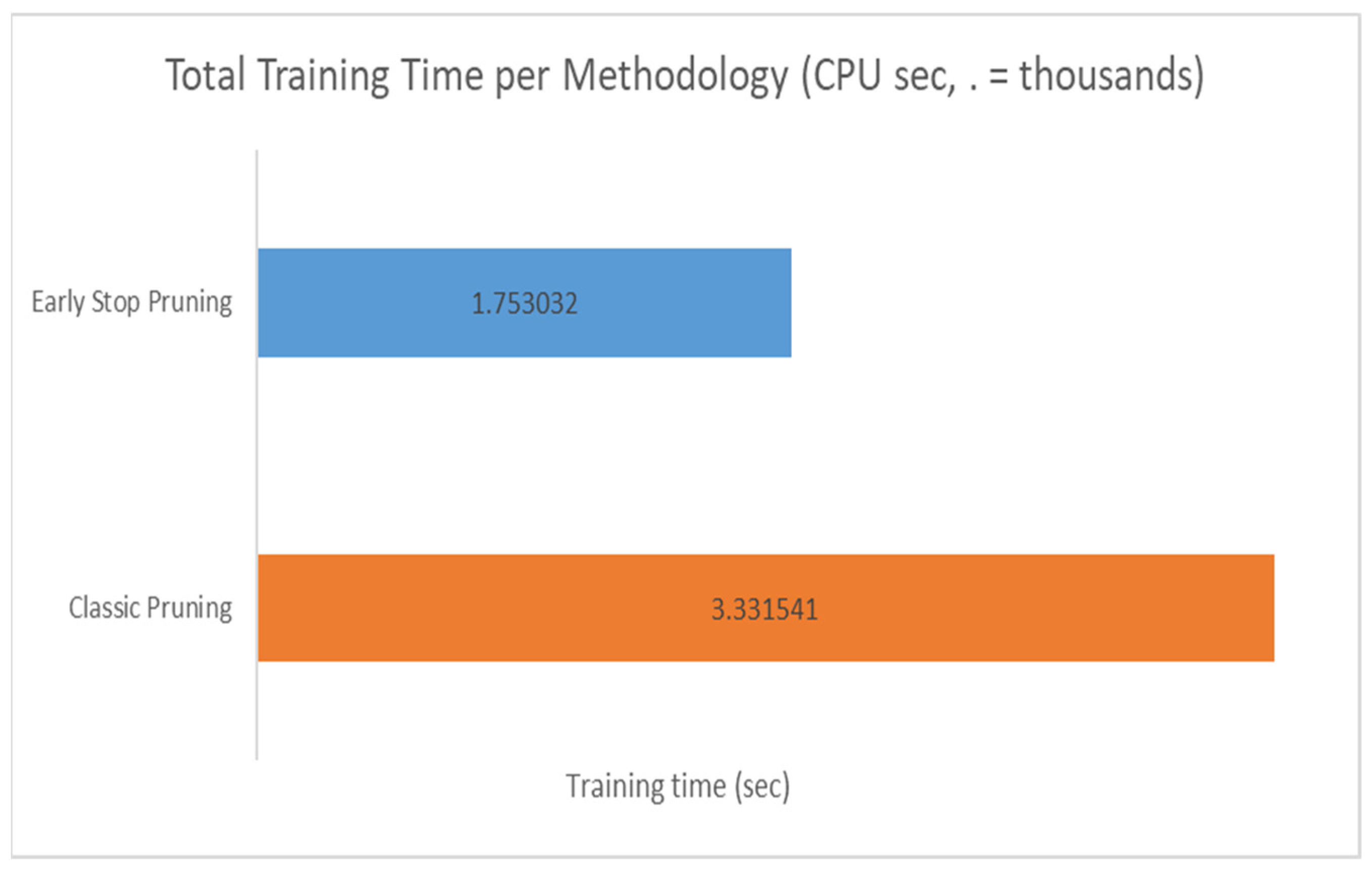
summarizes the average statistical metrics across the six time windows of the first five months of 2020, while Figure 5 illustrates the computational efficiency, expressed in terms of the computational requirements of the Classic and Early Stop Pruning methods.

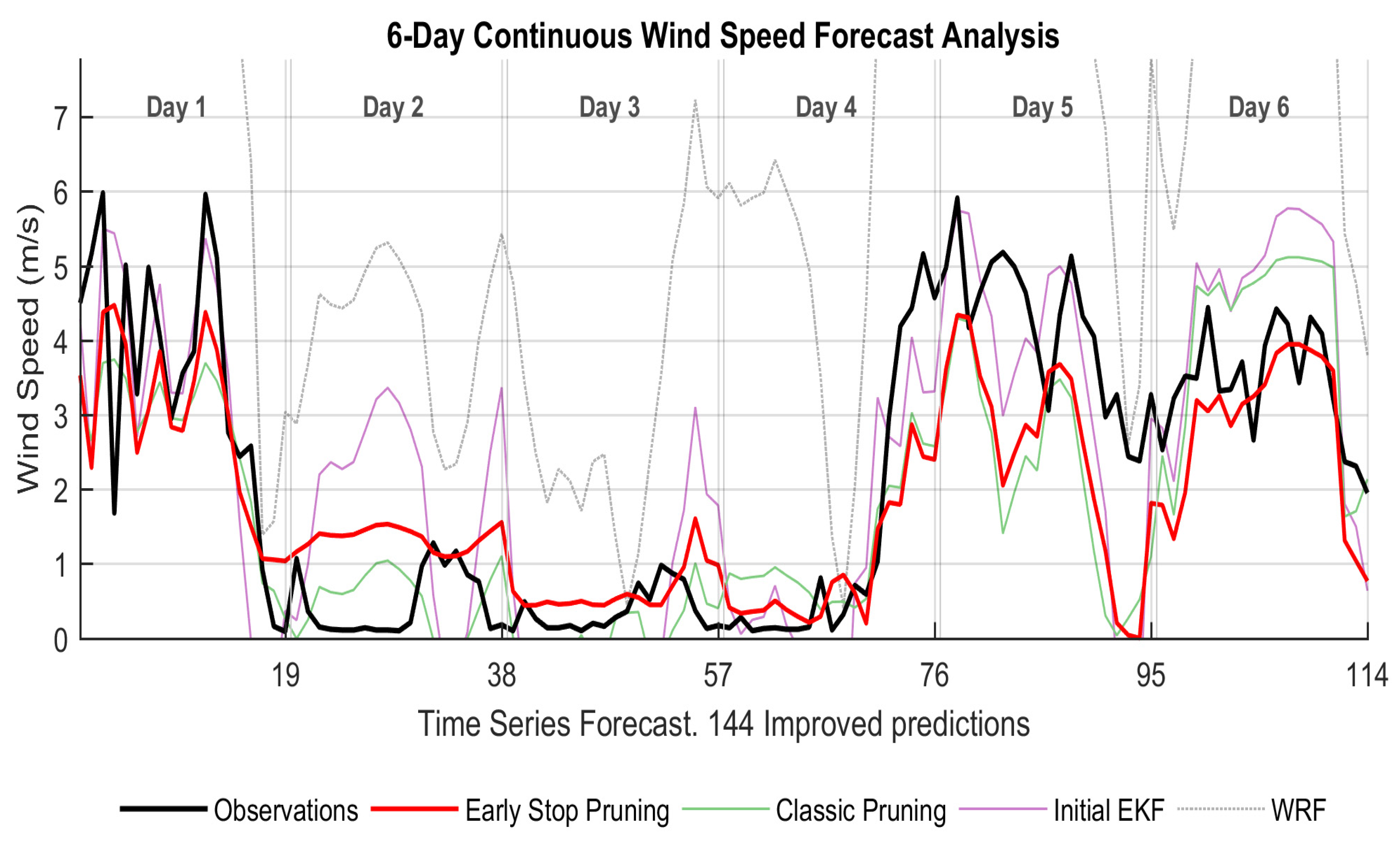
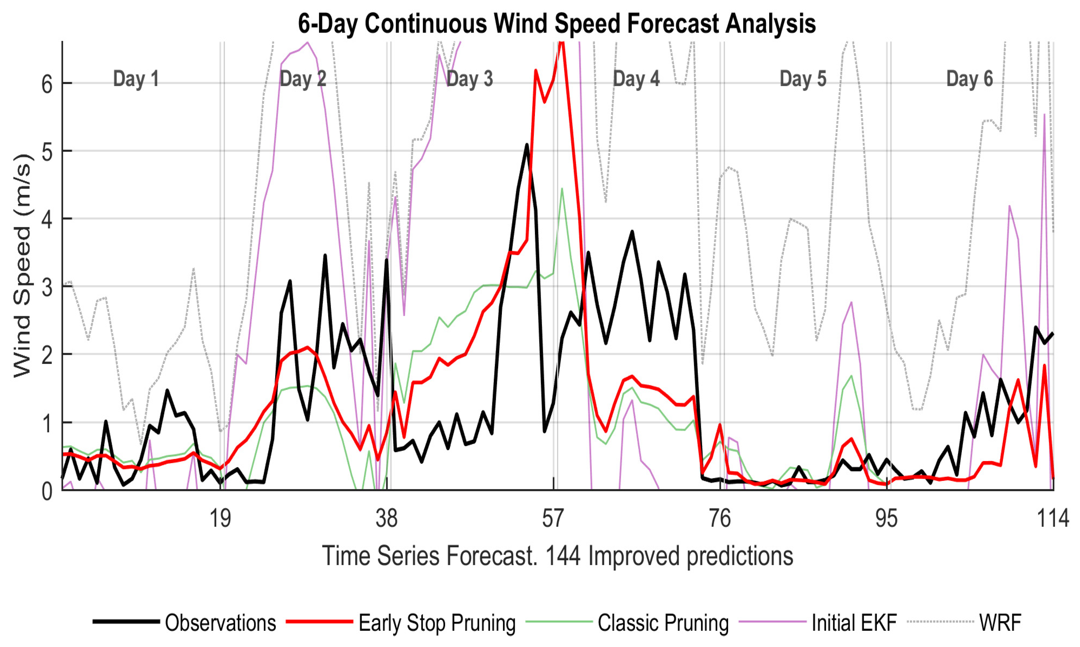
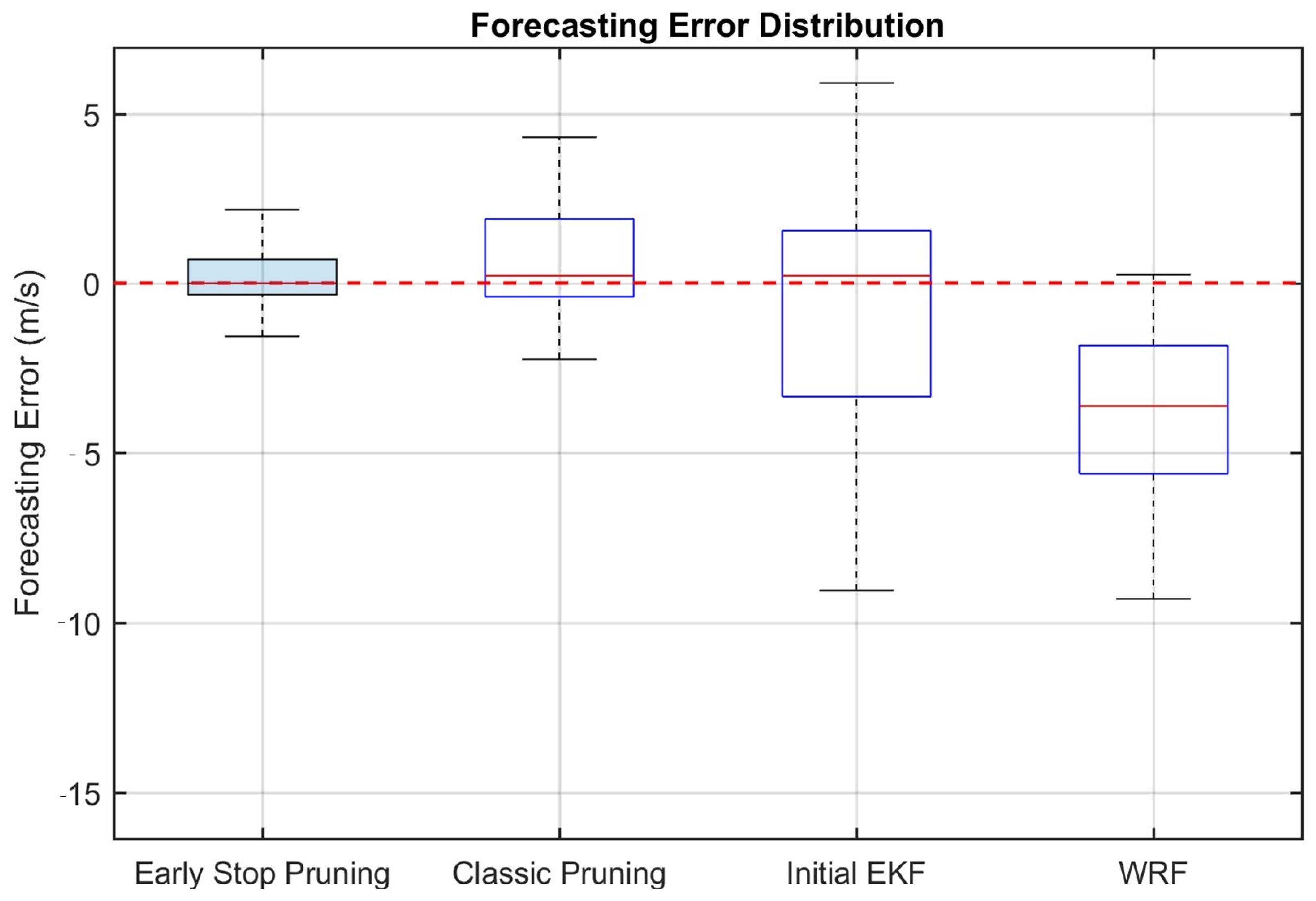
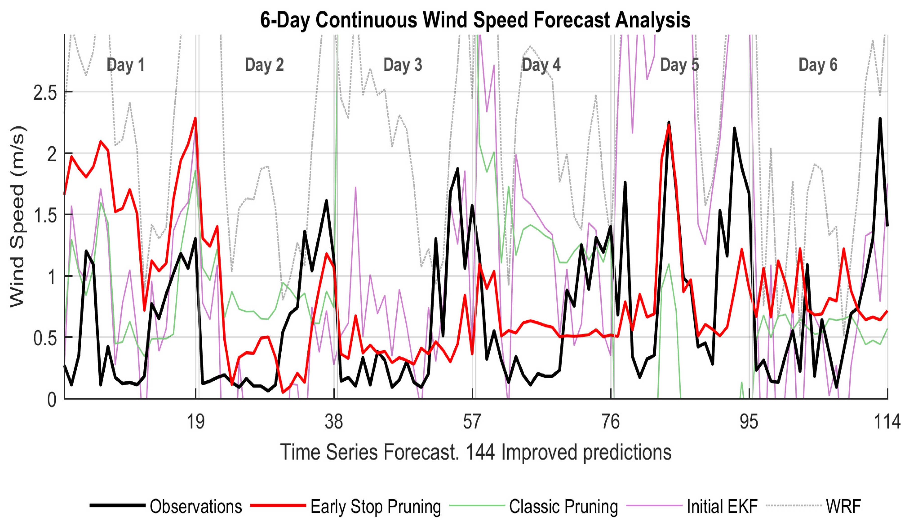
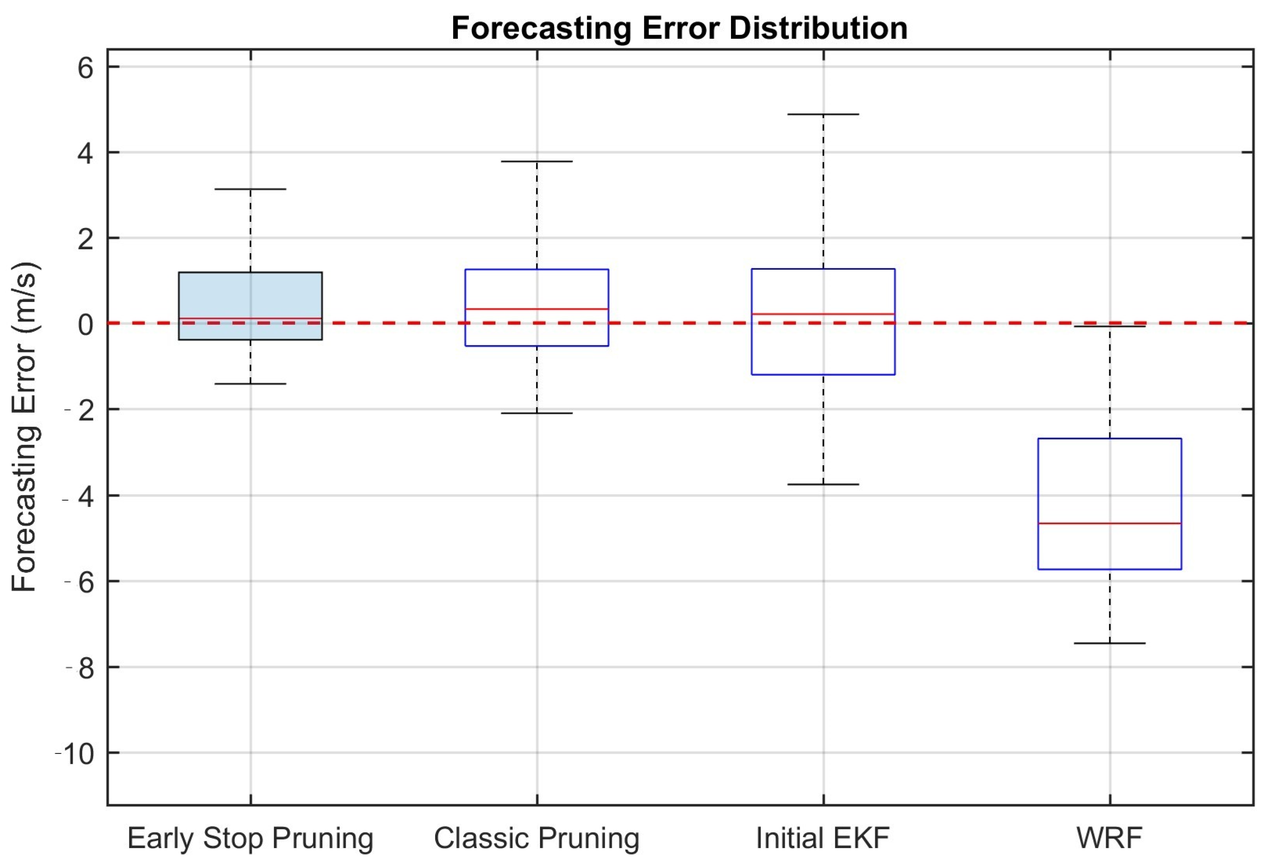
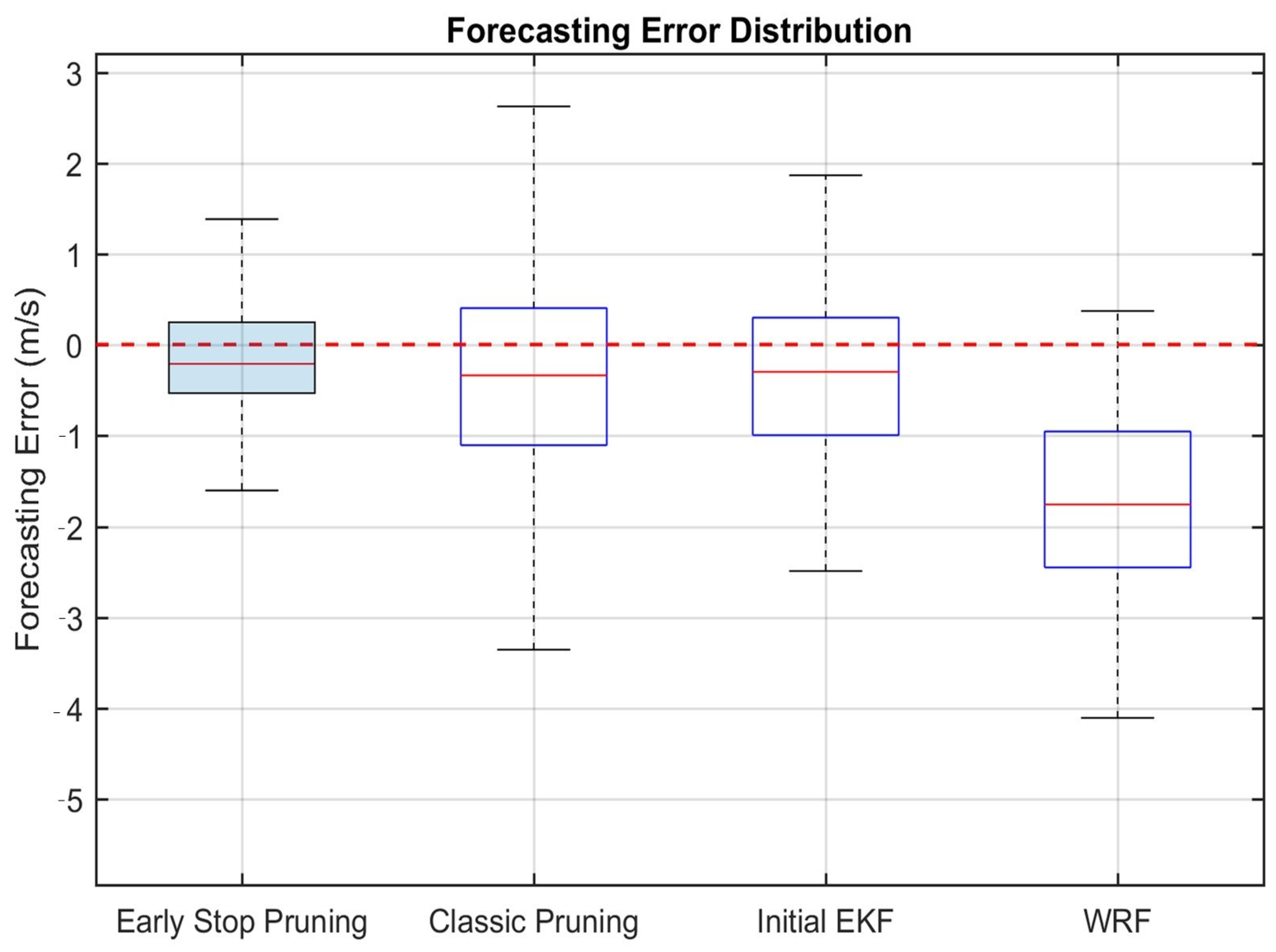
Figure 6, Figure 7 and Figure 8 depict the time series forecasts, and Figure 9, Figure 10 and Figure 11 present the corresponding boxplots of the forecasting errors (observation-forecast) for January, March, and May. These diagrams provide a visual comparison of forecast accuracy across the different methods and study periods, along with the corresponding quantitative assessment of error distributions. Specifically, the time series describes to what extent the produced forecasts capture the distribution of the weather parameter under study, while the boxplots indicate the forecast quality by measuring the variability of the forecast error.

Starting from the first week of each month, the time-window process is applied sequentially, producing consecutive daily forecasts, resulting in six forecasted days. Therefore, the horizontal axis in Figure 6, Figure 7 and Figure 8 presents these forecasted days, rather than the entire monthly period.

The overall evaluation period spans the first five months of 2020 (January–May), covering a wide range of atmospheric conditions and significant variability in wind patterns across 570 forecast instances (5 months × 6 days × 19 h). However, January, March, and May are selected as representative cases, as they effectively capture the diversity of the prevailing meteorological regimes (winter: Jan synoptic dominance; spring: Mar/May thermal/local influences). The terms Observations, Early Stop Pruning, Classic Pruning, and Initial EKF refer to the recorded data, the proposed approach, the classical pruning technique, and the initial hybrid EKF scheme, respectively. Finally, all examined approaches are trained under identical conditions, including the same number of epochs, identical pruning threshold and scaling factor, and the same training and validation datasets.

The comparative assessment of the statistical metrics, as presented in Table 2, reveals the enhanced predictive capabilities of the Early Stop Pruning method across all timeframes under consideration. A key observation is the substantial decrease in systematic error (BIAS). While the unrefined WRF model demonstrates a considerable and persistent overestimation of wind speed—exemplified by values as high as −4.24 m/s in February—the proposed methodology effectively reduces the BIAS to 0.3356 m/s in February and adjusts it to a value remarkably close to zero in other months (e.g., 0.0497 m/s in March and −0.0481 m/s in April). Consequently, this indicates that the suggested approach successfully mitigates the intrinsic “offset” of the physical model, thereby yielding nearly unbiased forecasts.

Furthermore, the evaluation of non-systematic errors through the MAE and RMSE metrics confirms the robustness of the proposed strategy. The Early Stop Pruning achieves the lowest MAE in the vast majority of cases, reaching a minimum of 0.58 m/s in May, which highlights its high precision in hourly intervals. More importantly, the notable decrease in RMSE compared to both the Initial EKF and the Classic Pruning (e.g., 0.94 m/s vs. 1.82 m/s in January) suggests that the proposed model is less prone to large forecasting outliers.

Quantitatively, the proposed approach achieves significant reductions, with RMSE reductions ranging from approximately 60% to 78% and MAE reductions between 65% and 80%, depending on the examined period, when compared to the initial WRF model output. This effectively bridges the gap between coarse physical simulations and local-scale observations. These significant enhancements can be partly attributed to the inherent limitations of the WRF model, which introduce systematic and non-systematic errors that affect the quality of its forecasts. Such errors arise from approximations in physical parameterizations, boundary conditions, and model resolution, leading to biases and reduced accuracy, particularly under complex atmospheric conditions.

Compared to the Classic Pruning technique, the Early Stop strategy generally leads to lower errors, although minor deviations may occur in specific cases. These findings, in conjunction with the computational efficiency analyzed in Figure 5, indicate that the double-criterion early stopping pruning not only mitigates overfitting, ensuring high-precision and stable final forecasts, but also leads to reduced computational requirements, making it suitable for real-time applications.

The visual examination of the time series diagrams (Figure 6, Figure 7 and Figure 8) confirms the superiority of the Early Stop Pruning method compared to other techniques. The proposed approach (red line) accurately reflects the observed data (black line), successfully avoiding the major overestimations seen in the raw WRF model (gray line) and the instabilities in the Initial EKF (purple line). In particular, during times of rapid wind speed changes—like Day 4 in February and Day 3 in March—the Early Stop method demonstrates a better ability to adapt to sudden shifts while maintaining a smooth and realistic forecasting trend. In contrast, the Classic Pruning (green line) often displays either delayed responses or unnatural swings during these transition periods.

A key benefit of the Early Stop Pruning strategy is its ability to effectively capture wind speed maxima events. In the 6-day continuous diagrams, the proposed model accurately represents peak wind speed values, usually with smaller “overshooting” or “undershooting” than the ones found in the Initial EKF and the raw WRF data. While the WRF model often makes unrealistic predictions, the Early Stop method connects the forecast with the physical limits of the local environment. During low wind speed periods, the proposed system shows strong stability, while the Classic Pruning often experiences erratic changes when wind speeds are near zero. The double-criterion approach ensures that the neural network maintains adequate structural complexity to accurately model low-wind conditions while removing unnecessary neurons that could add noise.

The analysis of error distribution (Figure 9, Figure 10 and Figure 11) supports these conclusions. Early Stop Pruning shows the most concentrated error distribution, with the Interquartile Range (IQR) being the narrowest among all the models compared. Furthermore, the median value closely matches the zero-error dashed line. This visually confirms that the proposed method effectively removes systematic bias and ensures high forecast consistency by significantly reducing the variance of the residuals. Additionally, the decrease in forecasting outliers is clear in the boxplot diagrams, where the “whiskers” of the proposed method are much shorter. In the March dataset, Early Stop Pruning keeps the error range within an exceptionally tight envelope. This stability, along with the previously analyzed computational efficiency, establishes the proposed method as a reliable option for real-time applications, ensuring accuracy across the entire operational range without high computational costs.

Summarizing the comparative analysis, the proposed double-criterion Early Stop Pruning technique demonstrates substantial improvements in meteorological time series forecasting, maintaining a computationally efficient framework. It yields consistent enhancements, as shown in Table 2, across all statistical performance metrics, effectively capturing the wind speed distribution, including periods of rapid temporal variability and abrupt transitions, thereby providing an accurate representation of maximum wind speed events. These findings indicate the consistent superiority, particularly in terms of significant bias reduction and improved MAE and RMSE values, highlighting its efficiency under varying conditions. Additionally, it should be highlighted that the observed improvements are consistent across all examined time periods, indicating that the performance gains are systematic rather than due to random fluctuations, with no notable variability observed during repeated executions of the training process.

Furthermore, the proposed methodology preserves a significantly greater segment of the network, constraining the reduction to a mere 2% to 13%, maintaining the critical non-linear mapping functionalities essential for modeling fluctuating wind patterns. This data-driven “intelligence” mitigates the excessive pruning seen in the conventional model, guaranteeing the network’s continued resilience in capturing the intricate dynamics revealed through time series analysis.

Importantly, the proposed hybrid scheme addresses a critical limitation of classical Kalman Filter-based approaches. Although traditional Kalman filtering is highly effective in reducing systematic bias, it often exhibits limited capability in reducing the variability of the forecast error, as measured by the RMSE and MAE, particularly in highly stochastic environments such as wind speed forecasting [40,41]. The suggested strategy, on the contrary, goes beyond that simple bias correction, improving both generalization and stability through the combined use of statistical and machine learning tools, leading to a more robust, balanced, and reliable forecasting performance compared to conventional methodologies.

4. Conclusions

In this study, a novel hybrid methodology was developed to enhance the accuracy of wind speed forecasting by integrating a Hybrid Extended Kalman Filter with an “Early Stop Pruning” mechanism. The proposed approach addresses the inherent limitations of Numerical Weather Prediction models, such as the WRF, which often exhibit increased forecast errors due to local topographic and climatic complexities.

The core contribution of this work lies in the development of a sequential pruning strategy that operates dynamically during the learning phase. By employing a dual-criterion evaluation based on validation error and the trace of the error covariance matrix, the model achieves a refined neural architecture that minimizes overfitting while maintaining high computational efficiency.

The obtained results demonstrate a significant improvement in forecasting performance. Specifically, the proposed approach reduces the RMSE and MAE up to 78% and 80%, respectively, compared to the raw WRF output. Furthermore, the BIAS was effectively neutralized, bringing the systematic error remarkably close to zero, indicating that the proposed hybrid scheme effectively constrains both types of forecast error. From a computational perspective, the “Early Stop” mechanism reduced the training time by nearly 50% compared to standard pruning methods, confirming its suitability for real-time operational applications. Overall, the proposed methodology provides a robust and efficient solution for wind energy forecasting.

Future research will focus on comparing the suggested hybrid scheme with modern deep learning architectures, such as Long Short-Term Memory (LSTM) and Gated Recurrent Units (GRUs), to further assess its performance and generalization capabilities.