Elastic Patterns: A Deformation-Based Approach to Interpretable Classification

Abstract

Elastic Patterns are presented as a novel approach to prototype-based pattern classification that integrates concepts from cognitive psychology, fuzzy logic, and physics. Traditional prototypes are revisited through their different formulations: psychological prototypes as central category elements, Fuzzy Prototypes addressing vagueness, and Deformable Prototypes incorporating elasticity to adapt to data variability. Elastic Patterns extend these ideas by representing each parameter as an independent elastic component, conceptualized as springs, which deform to fit new cases while minimizing deformation energy. Elastic Patterns operate at two levels: parameter-level deformation, measured through axial strain, and pattern-level deformation, expressed as cumulative deformation energy. This structure enables a transparent and adaptive recognition process, where classification is achieved by selecting the pattern requiring the least energy to deform. A case study on the MNIST dataset validates the proposal, achieving approximately 80% accuracy and reducing the need for extensive preprocessing. These results indicate that Elastic Patterns offer a promising alternative to conventional methods, combining interpretability, adaptability, and physical grounding in pattern recognition tasks.

1. Introduction

This paper presents a multidisciplinary approach to pattern recognition in elastic modeling. The proposed framework integrates concepts that have been successfully applied across different domains, using the notion of Prototype as a unifying element. Specifically, the concept of Prototype is presented from from different perspectives: cognitive psychology, where the notion of Prototype has been used to be able to group concepts in a simple way as the central axis of a category; fuzzy logic, through the concept of Fuzzy Prototypes, presents the notion of Prototype as a fuzzy scheme; and engineering, where Deformable Prototypes introduce adaptability through physical principles. Once these have been presented, the conceptualization of Prototype is also presented from a point of view closer to engineering, by means of the approach of Deformable Prototype, which recovers the conceptualization of Prototype as a central element of a category but enabling deformation-based recognition, presenting the prototype as a deformable element from the physical point of view, for which reason some similar basic physical concepts are also presented.

In prototype theory, categories are not assumed to exist as fixed entities in the external world. Instead, they are regarded as cognitive constructs that emerge from human perception. This perspective allows categories to be flexible and context-dependent, which is particularly relevant for modeling real-world data. The proposed Elastic Pattern framework builds on this idea by representing categories as Deformable Prototypes rather than rigid class definitions.

Recent advances in interpretable machine learning and prototype-based methods have highlighted the importance of transparent and physically meaningful models for classification tasks. In this context, the proposed approach is positioned within a growing body of work that seeks to balance performance with interpretability and conceptual clarity.

Based on the concepts discussed above, we introduce the notion of Fuzzy Prototypes, which has been widely applied as an improvement over previous approaches. This notion revisits prototyping within a fuzzy framework and incorporates the idea of Deformable Prototypes, allowing the prototype to adapt its structure. Building upon these foundations, we subsequently present a new framework extending Deformable Fuzzy Prototypes, namely Elastic Patterns.

Since prototype-based learning, fuzzy modeling, and interpretable machine learning have evolved along partially independent research directions, each addressing different aspects of classification and representation. Prototype-based methods focus on similarity to representative elements, fuzzy approaches introduce graded membership to handle uncertainty, and interpretable models aim to provide transparency in decision-making processes. Recent developments have sought to bridge these perspectives by combining structured representations with meaningful similarity measures. Within this context, the proposed Elastic Pattern framework can be understood as a unifying approach that integrates these lines of research. By introducing a deformation-based similarity grounded in physical principles, it extends traditional prototype-based formulations and provides a coherent interpretation of classification in terms of energy minimization. This perspective complements existing approaches while offering a physically interpretable mechanism for modeling variability within and across classes.

1.1. Comparative Analysis of Related Frameworks

The proposed EP framework is conceptually grounded in several research domains, including cognitive psychology [1], fuzzy logic [2], physics, and engineering. Each of these fields provides a distinct perspective on the notions of prototypes, similarity, and transformation.

In cognitive psychology, prototype theory describes categories in terms of representative exemplars, where membership is determined by similarity to a central prototype [1]. In fuzzy logic, this idea is formalized through graded membership functions, allowing elements to belong to categories with varying degrees [2]. In contrast, physics and engineering introduce the notion of deformation and energy, where transformations between states are quantified through measurable physical quantities.

The EP framework integrates these perspectives by combining prototype-based representation with a deformation-based similarity measure. In this context, classification is interpreted as an energy minimization process, where the most compatible prototype is the one requiring the least deformation.

To clarify these relationships,

Table 1. Comparative analysis of related frameworks across different research domains.

Aspect	Cognitive Psychology	Fuzzy Logic	Physics	Engineering	EP
Core concept	Prototype	Fuzzy set	Physical state	System model	Deformable prototype
Representation	Exemplar-based	Membership function	State variables	Parametric model	Elastic parametric representation
Similarity measure	Perceptual similarity	Degree of membership	Energy difference	Error or cost function	Deformation energy minimization
Transformation	Conceptual shift	Membership variation	Deformation	System response	Elastic deformation of parameters
Interpretability	High (intuitive)	Moderate	High (physical meaning)	Moderate	High (explicit and physically grounded)
Mathematical formalization	Limited	Strong	Strong	Strong	Integrated (multi-domain formulation)
Key references	[1,3,4]	[2,5,6,7]	[8,9,10]	[11]

provides a structured comparison of the main concepts across these domains.

The final column explicitly highlights how the proposed framework extends the contributions of the referenced domains. In particular, it combines the prototype-based reasoning introduced in cognitive psychology, the graded representation of fuzzy logic, and the deformation and energy principles derived from physics and engineering into a unified classification model.

The Elastic Pattern framework can be interpreted as a unifying model that bridges these domains by embedding prototype-based reasoning into a physically grounded deformation process.

1.2. Summary of Contributions

The main contributions of this work can be summarized as follows:

• A novel classification framework based on Deformable Prototype representations, referred to as Elastic Patterns, in which each class is modelled through a parametric structure inspired by physical systems.
• A unified formulation that integrates concepts from cognitive psychology, fuzzy logic, and physics, enabling a coherent interpretation of classification in terms of similarity, membership, and energy-based deformation.
• An ante hoc interpretable modeling approach, where classification decisions arise from explicit transformations of prototypes, allowing the reasoning process to be directly analyzed and understood.
• A deformation-based similarity measure, in which the affinity between an input instance and a class is quantified through the energy required to adapt the corresponding elastic prototype.
• A methodology that reduces dependence on task-specific preprocessing by modeling variability within the representation itself, rather than through external transformation pipelines.
• An experimental validation on both image-based and structured datasets, demonstrating the applicability of the proposed framework beyond standard benchmark scenarios.

These contributions collectively position Elastic Patterns as an alternative framework that prioritizes interpretability and conceptual transparency while maintaining a competitive and flexible modeling approach.

1.3. Notation and Definitions

For clarity and consistency, the main symbols, indices, and abbreviations used throughout the manuscript are summarized in this section.

1.3.1. Symbols

The main symbols used throughout the manuscript are as follows:

• x: Input instance (observed data sample).
• $p_{i,j}$: j-th parameter of prototype ${\mathbf{p}}_i$.
• p: Prototype representing a class or category.
• $x_j$: j-th component of the input vector.
• ${\epsilon }_i$: Axial deformation associated with the i-th component.
• $p1$, …, $pn$: A prototype defined by its parametric representation.
• $m_i$(v, $p1$, …, $pn$): Matching function of an input x over a prototype.
• S(x,p): Similarity measure between input x and prototype p.
• ${\epsilon }_{i,j}$: Axial deformation of parameter j for prototype i.
• $E_i\left(x\right)$: Total deformation energy associated with prototype i for input x.

In some classical formulations, particularly in the context of Deformable Prototypes, the term object is used to denote the input. In this manuscript, this concept is consistently represented by the variable x.

1.3.2. Indices

The main indices used throughout the manuscript are as follows:

• i: Index over class prototypes.
• j: Index over feature dimensions.

1.3.3. Derived Quantities

The axial deformation is defined as:

$${\epsilon }_{i,j}={\displaystyle \frac{x_j-p_{i,j}}{p_{i,j}}}$$

(1)

The total deformation energy is given by:

$$E_i\left(x\right)={\displaystyle \sum _{j=1}^n}{\epsilon }_{i,j}$$

(2)

1.3.4. Acronyms

The main acronyms used throughout the manuscript are as follows:

• EP: Elastic Patterns.
• ML: Machine learning.
• FCM: Fuzzy C-Means.
• KNN: k-Nearest Neighbours.

2. Related Work

As the complexity of conceptual categories increases, classification methods must handle increasingly complex patterns. This has encouraged the development of approaches capable of modeling uncertainty by integrating concepts from multiple domains, such as fuzzy logic, prototype theory, and energy-based modeling. These methods have proven effective in representing degrees of class membership rather than relying on binary decisions. Current approaches in interpretable machine learning have emphasized the importance of models that are transparent by design rather than relying on post hoc explanations [12].

For example, a fuzzy inference system for wafer defect classification [13], where patterns are assigned to classes based on a degree of conformity. This approach, in which a sample is classified as defective or not, is conceptually aligned with the basic concept of fuzzy logic, where an element does not belong entirely to a class, thus measuring the degree of conformity with the wafer that is being classified as defective or not. This is conceptually similar to EPs, as both approaches rely on deformation energy to classify a sample into a category, similar to the degree of conformity proposed by this approach.

Other proposals that incorporate concepts similar to EPs include the proposal for characterizing the boundary data of a class or cluster, such as the improved FCM approach proposed [14], where each central element of the cluster acts as a Fuzzy Prototype that adapts to classify elements within a category/cluster, the Fuzzy Prototypes proposed in this approach are conceptually similar to the representation of the parameters of EPs and how they deform within a category to classify an element of the EP.

Recent surveys have highlighted the growing relevance of prototype-based approaches within explainable artificial intelligence frameworks [15]; prototype-based methods have been widely explored as interpretable alternatives to black-box models, where classification is based on similarity to representative elements. There is a growing shift from post hoc explainability towards intrinsically interpretable models, motivating alternative approaches to classification [16,17]. In this context, intrinsically interpretable approaches aim to provide transparent and reliable decision mechanisms without relying on post hoc explanations [18].

Emerging advances in physics-informed machine learning have demonstrated the value of incorporating physical principles into data-driven models to enhance both interpretability and structural coherence [19]. These approaches emphasize the use of physically meaningful quantities, such as energy and deformation, to guide the modeling process. In this context, classification can be interpreted not merely as a statistical task, but as a transformation governed by underlying structural constraints.

Energy-based formulations have been proposed as an alternative paradigm for modeling complex systems, where compatibility is expressed through an energy function [20]. One example of a proposal is based on calculating energy consumption during the movement of a mobile robot [21]. This approach defines an energy coefficient, calculated based on motor current and velocity. This coefficient represents different energy patterns to adapt to different surfaces, subsequently using a probabilistic classifier to classify the current surface with previously known surfaces. This approach aligns with EP, as both approaches make use of the formulation of energy cost, where a system, the mobile robot or an EP, requires energy to classify a sample, the terrain on which the robot moves, or the classification of new samples by EP.

So, the EP approach constitutes a novel contribution because it integrates multiple concepts from different fields, such as cognitive psychology, fuzzy logic, and the physical characteristics of materials. Although these concepts or methods have been proven in multiple approaches, they are not usually used together. This is mainly due to the following reasons:

• EPs adopt a prototype-centered view of categorization from cognitive psychology, as introduced by E. Rosch [1], in which categories are organized around representative central elements rather than strict boundaries.
• EPs incorporate fuzzy logic, following L. Zadeh’s conceptualization [2], to model gradual class membership and handle uncertainty in a principled manner, combined with the energy needed to deform the parameters that form the prototype based on physical characteristics, thus also measuring the degree of belonging to a class.
• EPs draw inspiration from deformable patterns, such as those proposed by H. Bremermann [11], by allowing class representations to adapt their internal structure when confronted with new samples.
• EPs can be naturally framed within ante hoc XAI, as interpretability is embedded directly in their formulation rather than obtained through post hoc analysis. The classification process is explicitly defined in terms of parameter deformations and their associated energy, allowing each decision to be traced and understood in a transparent manner.

Finally, and most distinctively, EPs introduce a physically grounded simulation based on elastic elements, springs, where classification is based on the minimization of a deformation energy.

3. Intersection of Cognitive Psychology, Fuzzy Logic, Engineering and Physics

3.1. Prototypes in Cognitive Psychology

The process by which humans group or classify elements of the real world is a process that has been widely studied and debated within cognitive psychology, with one of the most established theories being that proposed by the psychologist Eleanor Rosch (E. Rosch). E. Rosch proposes that the categorizations that we humans make are actually non-existent in the real world on many occasions; for example, if we review one of the most celebrated paragraphs of the book The Art of War: A cartload of enemy grain that feeds your army is equal to 10, we can deduce that there are two categories—own grain, with a value of one, and enemy grain, with a value of 10—which is a categorization based on human perception, while the properties of the classified elements, grain, are practically similar, or there may be other categories, such as the type of grain, which have been ignored.

According to E. Rosch, the creation of categories in human thought takes place according to two principles [4]:

• The main objective of categorizing the elements existing in the real world is to offer the greatest possible information with the least possible effort. E. Rosch calls this principle Cognitive Economy.
• People tend to perceive the real world as structured information, and not as a set of unstructured information, in other words, as unstructured individual elements. However, the reality depends largely on who perceives it; each person, depending on their experiences, knowledge, etc., will tend to perceive reality and structure the information received in one way or another. For example, a veterinarian with extensive knowledge, for example, of feathers, fur, etc., knows that wings are more closely related to feathers than to fur. E. Rosch calls this principle Structured Perceived World.

Following the principle of cognitive economy, E. Rosch affirms that categories tend to be formed separately from each other, but at the same time as close as possible; a way of being able to carry out this way of constructing the categories is through the use of formal criteria, necessary and sufficient, for the creation of the categories. In many cases, this approach is commonly referred to as the logical approach [4]. A common criticism of this approach is that categories naturally do not have clearly defined boundaries despite the criteria used to create them, as perceived elements do not necessarily have a continuous set of attributes, which can be understood as meaning that not everyone perceives (or assigns) the same attributes to all perceived elements.

E. Rosch also proposes that another approach to understanding and creating categories can be based on very clear cases; the perceived information is structured into classes by the structural correlations among the attributes of the case, their structure and how they relate to each other. This approach is often referred to as the prototype approach. Therefore, E. Rosch defines the prototype as those cases that are clearer when defining the belonging to a category; thus, it is possible to understand the prototype as the central element of a category and to measure the belonging to this category of other elements according to the similarity with the prototype [4].

E. Rosch points out that it is common that the interpretation of the creation and understanding of categories on the basis of the two previously proposed approaches—the logical approach, which defines the category on the basis of necessary and sufficient criteria to define the category, and the prototype approach, which uses very clear cases to define the degree of belonging to the category—tends to be understood as mutually exclusive, although this does not have to be so, and in certain cases, they can be understood as complementary. For this purpose, E. Rosch relies on the concept of reasoning; reasoning is traditionally defined as conscious deliberation, but E. Rosch adds that reasoning can also be conscious deliberation. Rosch adds that reasoning can be any form of inference, deliberation or automatic/unconscious response, so both existing approaches to defining and creating categories can make use of reasoning. The logical approach will make use of reasoning to determine the logical structures of perceived elements, and the prototype approach will make use of reasoning using reference cases (prototypes) [22]. E. Rosch also clarifies that both types of reasoning are complementary. Rosch also clarifies that both types of reasoning, the one used in the logical approach and the one used in the prototype approach, begin to develop in childhood, and depending on what is more convenient in each case, one or the other approach is used intuitively.

Although it is true that the logical approach is traditionally the most used, due to the ease of understanding a simple scheme of attributes, the prototype approach, which is based on similarity, is more interesting for this work, so this approach is not examined further in this work. E. Rosch states that there are three ways of categorizing perceived elements using the prototype approach, and these are set out below [22]:

• Reasoning on the basis of cases, examples or events that may be in opposition to what might be inferred from general knowledge.
• Inference from salient reference points within an organized domain.
• Reasoning using representativeness. E. Rosch states that the prototyping approach, as previously stated, is based on clear cases and how similar they are to others, so a wider range of cases in which prototypes are used is needed.

As has been described in the previous list, the last case is the most common, so going deeper into it, other authors have proposed that prototypes are the best way to represent the relationship of representativity between different perceived elements [23]; representativity can be understood as the relationship between a process/model and an instance/event, and this relationship of representativity can be defined for the following cases:

1.

A value and a distribution. Representativeness is defined as a frequency or relative statistic perceived as the mean, median or mode of a distribution. The category artificial tends toward this kind of representativeness relationship [24].

2.

An instance and a category.

3.

An instance and a population.

4.

An effect and its cause, thus defining representativeness through the beliefs of the causes. A common criticism of this case is that it may resemble the logical approach to creating categories.

Research with common semantic categories is of types 2 and 3; e.g., a real-world item such as a robin can be treated as an instance of the category birds or as a sample of birds. Prototypes as reference points for categories can be representative either because the most representative members of the categories are taken as prototypes, or because these members are prominent points in a domain and the category tends to surround them and form around the prototype, thus making them representative of that category [22].

3.2. Other Conceptualizations of the Prototypes

The concept of prototype is universally understood as a very representative element of a class or category, i.e., a prototypical element is an element widely used and through which a class or category can be easily recognized, this notion has been used from different approaches, several of them relying on cognitive psychology.

Based on definitions, such as E. Rosch’s proposal [1] in the context of the study of cognitive concept organization, in the center of a category is the prototype, which describes the characteristic properties of the elements of that class. Based on this, it can be established that not all members of a class are equivalent, and some will be better examples and more characteristic of the category than others.

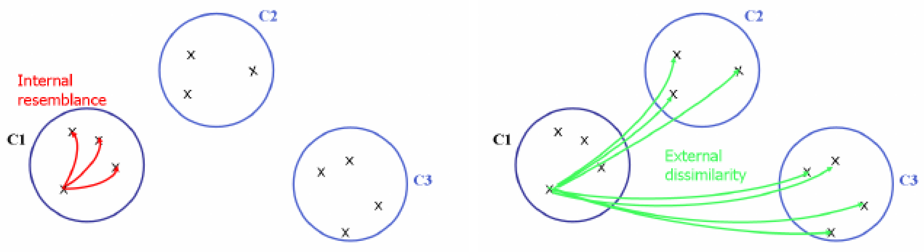
Based on this idea, some authors proposed that the degree of typicality of an element depends positively on its total resemblance to other objects of its class (internal resemblance) and on its total dissimilarity to objects of other classes (external dissimilarity) [25]; a graphical representation of this is shown in Figure 1.

Based on this approach to weigh the degree of typicality of an element and using fuzzy logic to adapt to the concept of degree of prototypicality, a method for the construction of Fuzzy Prototypes was proposed [25]:

1.

Calculate the internal resemblance degree of an element with the rest of the elements of the category and its external dissimilarity degree with the elements that are outside of the category.

2.

Aggregate the internal resemblance and the external dissimilarity degrees previously calculated to obtain the typicality degree of the element.

3.

Aggregate elements that have a sufficient degree of typicity, commonly established by a threshold.

In the context of prototype-based classification, it is useful to distinguish between internal and external similarities. Internal resemblance refers to the degree of resemblance between an instance and the prototype of its assigned category; it captures the internal coherence of the category and reflects how well the instance fits within it. External dissimilarity, by contrast, describes the relationship between an instance and prototypes of other categories. This notion is particularly relevant in regions where class boundaries are not clearly defined, as it accounts for potential overlaps and ambiguities between categories. These two forms of similarity play a complementary role in classification. While internal resemblance supports the assignment of an instance to a category, external dissimilarity provides a measure of separation between competing categories.

3.3. Fuzzy Prototypes

In 1981, Osherson and Smith presented an interesting critique in which they argued that the fuzzy set approach does not provide a suitable solution to the problems we encounter when constructing a theory of prototypes [26]. One of Osheron and Smith’s criticisms is based on the fact that in conjunctive concepts, for example, a square plate, the application of the rules of combination for fuzzy sets leads to a contradiction when the conjunctive concept is more prototypical than a conjunction of its parts. This criticism was also made in 1975 by Paul Smith, who observed that, in certain cases, the degree of membership of an object x in the intersection of two fuzzy sets A and B can be greater than the degree of membership in A or in B [5].

For this point of criticism, L. Zadeh proposes the following explanation: When we are faced with a sub-normal fuzzy set, a fuzzy set in which the maximum degree of membership is less than 1, and when we focus on the intersection of the sets A and B, that is, A $cap$ B, which we can call C, tacitly C is being normalized by relativizing the degrees of membership of C with respect to the maximum degree of membership of A $cap$ B. By doing this, we are generating a normalized fuzzy set, Normalized(A ∩ B), which is not a subset of A and B; therefore, an object x can have a higher degree of permanence in this new normalized fuzzy set, Normalized(A ∩ B), than in A or in B [27].

Another aspect related to this issue is that, according to fuzzy set theory, the conjunctive combination is detailed by the operator when the combination is non-interactive [27]. There is now a broad consensus that there is no single formula for conjunction that is able to define the large number of different ways in which conjunction is introduced into concept formation and meaning representation.

It should also be noted that what could be understood as a failure of compositionality in conjunctive concepts. These, in natural language, are usually denoted in a phrase of the form NA, where N is a noun, and A is a descriptor of N, where this form NA is not the intersection of the denomination of N and A, no matter how the intersection is defined. Returning to the conjunctive concept square plate, taking back the example given above, N would be the noun plate, and A would be the adjective square. The reason behind this fact is that, in many cases, A is not a descriptor of N, but is instead an operation that modifies N to transform it into the denotation AN.

A simple example to understand this could be the notation of light aircraft, where in this case what is being applied is the operator light on the denotation aircraft rather than the intersection of the denotations aircraft and light. Also, what seems to fail in the compositionality in this example is that the result of interpreting light as a descriptor of plane is that it is really an operator being applied to plane.

Another criticism raised by Osheron and Smith is that in fuzzy set theory, the conjunction of the set A with its complement A’ may not be the complete universe of discourse. This is directly related to a long-running debate about the validity of the middle term exclusion principle [6,28]. L. Zadeh claims that this principle is not a valid proposition in fuzzy set theory, since it cannot be applied in circumstances where one is dealing with classes whose boundaries are not clearly defined.

Osheron and Smith also suggest that disjunctive concepts in fuzzy set theory can lead to counter-intuitive results, giving an example in which they present the concept of financial health and how they are directly related to the concepts of liquidity and investment and how the degree of membership of either or both of these directly affects the degree of membership of financial health [26]. According to L. Zadeh, the problem here lies in the way Osheron and Smith define the notion of financial health as a disjunction of liquidity and investment, a definition that does not reflect our intuitive perception of the relationship between these variables. Zadeh proposes to the authors that a way to adequately define the relationship between the concepts is by following the examples defined by L. Zadeh himself in other works [7].

Osheron and Smith also criticize the approach of inclusion in fuzzy set theory, proposing that the proposition all grizzly bears inhabit North America is counter-intuitively falsified by the existence of a squirrel on Mars. L. Zadeh argues that the origin of the problem in this case is not the concept of inclusion in fuzzy set theory, but the fact that in natural language, the quantifier everything is not usually understood in its strict logical sense. So, in general, the quantifier all must in natural language be understood as a fuzzy proposition that is close to unity. Taking this into account, making use of the notion of cardinality of fuzzy sets [27], and the use of a threshold, which eliminates the elements of the objects below it, L. Zadeh considers Osheron and Smith’s criticism on this point to be valid, although he also proposes, as a solution to this criticism, carrying out a borrosification of the concept of inclusion, which has already been carried out in other works.

L. Zadeh proposes that the criticisms and difficulties proposed by Oserhon and Smith can be resolved as he proposes to each of the criticisms above, although a more serious problem appears in the shortcomings of the standard version of prototype theory summarized by Oserhon and Smith, as this version takes up several key points:

• In prototype theory, a prototype is understood as a representative element that captures the central characteristics of a category, rather than as a strict member defined by necessary and sufficient conditions.
• The similarity between an instance and a prototype can be interpreted as a measure of how closely the features of the instance align with the characteristic attributes of the category. In this sense, proximity to the prototype corresponds to a higher degree of membership.

L. Zadeh proposes two criticisms of this theory:

• It is possible to argue that, in general, the prototype is not a member of the class.
• An object can be far from the prototype, according to some kind of metric or evaluation, and still belong entirely to a particular class.

So, in order to give a satisfactory definition of a prototype, L. Zadeh proposes that it should be compatible with the following principles [2]:

• A prototype is not a single individual object or even a group of objects of A. It is more appropriate to understand it as a fuzzy scheme in order to generate a set of objects that are approximately coextensive with A.
• The prototypicality is a problem of degree; this implies that the concept of prototype is a fuzzy concept.
• The notion of prototype is an opaque concept in the sense that, although it may be possible to define it clearly or by exemplification, it may not be possible to define explicit criteria for assessing the degree to which a scheme qualifies as a prototype.

L. Zadeh, with these postulates, affirms that the goal of formalizing the notion of prototype, according to the standard theory, is impossible. According to this, it may be necessary to admit a fuzzier demise in which the gain of information is achieved by defining the opaque concept of prototype in terms of a more fundamental approach, the idea of summary. The definition of this idea, which uses the notion of $delta$ summary, which is a succession of summaries, to generate a set of prototypes for a set of objects, is defined below. This particular definition is only a partial definition of the process by which the prototype concept is defined, and is more or less in the style of definitions based on the probabilistic summary idea [29]. The starting point for defining a population A of objects need not be distinct objects $u_1,u_2,\dots ,u_n$; rather, they are presented as a fuzzy multi-set. The difference between a multi-set and a fuzzy set is that the former can include identical objects. This definition of A is understood as an element $u_1$, with a degree of membership ${\mu }_1$; an element $u_2$, with a degree of membership ${\mu }_2$; and so on up to $u_n$, with a degree of membership ${\mu }_n$. To reflect the identical elements of A, we can define them as:

$$A={\displaystyle \sum _{i=1}^n}{\displaystyle \frac{{\mu }_i}{u_i}}{\mu }_i\in [0,1]$$

(3)

In this definition, ${\mu }_i$ is a real number, which represents the multiplicity of $u_i$, that is, the number of times that element is found in the fuzzy multi-set.

An example of how this can be done in a simple way is the following: suppose that A is a population of commercial planes, and a term in the form ${\displaystyle \frac{0.8}{6}}\ast u_2$, which means that in the population being used, there are six identical planes with the common descriptor $u_2$, and that the degree of compatibility of each plane $u_2$ is 0.8, with the concept labelled as a commercial plane.

The purposes underlying the assumption that A is a fuzzy multi-set are:

• As a multi-set, A, provides information about the distribution of the elements of A, this is a factor that influences the perception of prototypicality.
• As a fuzzy multi-set, the definition of the type ${\displaystyle \frac{{\mu }_n}{m_n}}\ast u_n$ also defines the degree to which each object $u_i$ conforms to A as a notion.

These degrees serve as clues to the characteristics that distinguish good examples from bad examples, which, as stated in E. Rosch’s theory of prototypes [4], is an important aspect in the definition of prototypes.

L. Zadeh defines that it is useful to stratify the representation of A, grouping the elements that have the same or similar degree of belonging, thus creating a stratification of A in a few levels. L. Zadeh proposes representing A with a stratification in three levels:

$$A={\displaystyle \frac{High}{A_{Good}}}+{\displaystyle \frac{Medium}{A_{Borderline}}}+{\displaystyle \frac{Low}{A_{Poor}}}$$

(4)

where:

• $A_{Good}$, $A_{Borderline}$ and $A_{Poor}$ are multiple fuzzy sets of good, borderline and bad examples respectively.
• High, Medium and Low are fuzzy numbers representing the fuzzy degrees of membership.

L. Zadeh also states that it is important to ensure that the lower the degree of membership associated with a stratum, the less weight it should have in the creation of the prototype. Starting with the stratum $A_{Good}$, for each object in this stratum, we partially summarize by removing one or more features, indicating that these features do not affect the goodness of that object. As a result of this partial summarization, some of the objects in $A_{Good}$ are transformed into identical (or nearly identical) objects. By grouping the objects in this way, their multiplicity will inevitably increase, and thus, the number of distinct objects in $A_{Good}$ is reduced. If this process is repeated an indeterminate number of times, one will end up with a maximally summarized object $PT\left(A_{Good}\right)$, which can be considered a prototype $A_{Good}$. Following the same method for the strata $A_{Borderline}$ and $A_{Poor}$, and any other possible strata that have been defined, we will obtain their respective prototypes, or more generally, a group of prototypes $PT\left(A_{Borderline}\right)$, $PT\left(A_{Poor}\right)$, etc. Therefore the prototype of A is a fuzzy set, and it is fuzzy in the sense that the prototype of A can be interpreted as an object that is a summary of the initial objects of a given population.

$$PT\left(A\right)={\displaystyle \frac{High}{PT\left(A_{Good}\right)}}+{\displaystyle \frac{Medium}{PT\left(A_{Borderline}\right)}}+{\displaystyle \frac{Low}{PT\left(A_{Poor}\right)}}$$

(5)

L. Zadeh states that, in essence, a prototype is defined with a fuzzy scheme for generating/recognizing the elements of a population of objects; his definition, unlike other more classical definitions of prototyping, does not include any precise criteria of prototypicality, as it attempts to address the imprecision in the intuitive perception of the concept of prototyping by creating a fuzzy set of prototypes rather than a single prototypical object.

Prototype theory, originating in cognitive psychology, describes categories in terms of representative elements that capture their central characteristics. In this framework, membership is not defined through strict boundaries but through similarity to a prototype. Fuzzy logic provides a formal counterpart to this idea by introducing membership functions that assign a degree of belonging to each element. This allows the intuitive notion of similarity in prototype theory to be expressed in mathematical terms.

Within this perspective, the similarity between an instance and a prototype reflects the degree to which the features of the instance align with the characteristic attributes of the category. Consequently, proximity to the prototype can be interpreted as a higher degree of membership, providing a direct link between cognitive and mathematical representations. This conceptual relationship serves as the basis for the formulation adopted in this work, where prototype-based reasoning is combined with a deformation-based similarity measure.

3.4. Deformable Prototypes

H. Bremermann (Hans-Joachim Bremermann) was a German–American mathematician and biologist who contributed several works in the field of pattern recognition, based on previous works such as neural networks; one of his most notable works, although remaining only at a theoretical level, was his proposal of Deformable Prototypes.

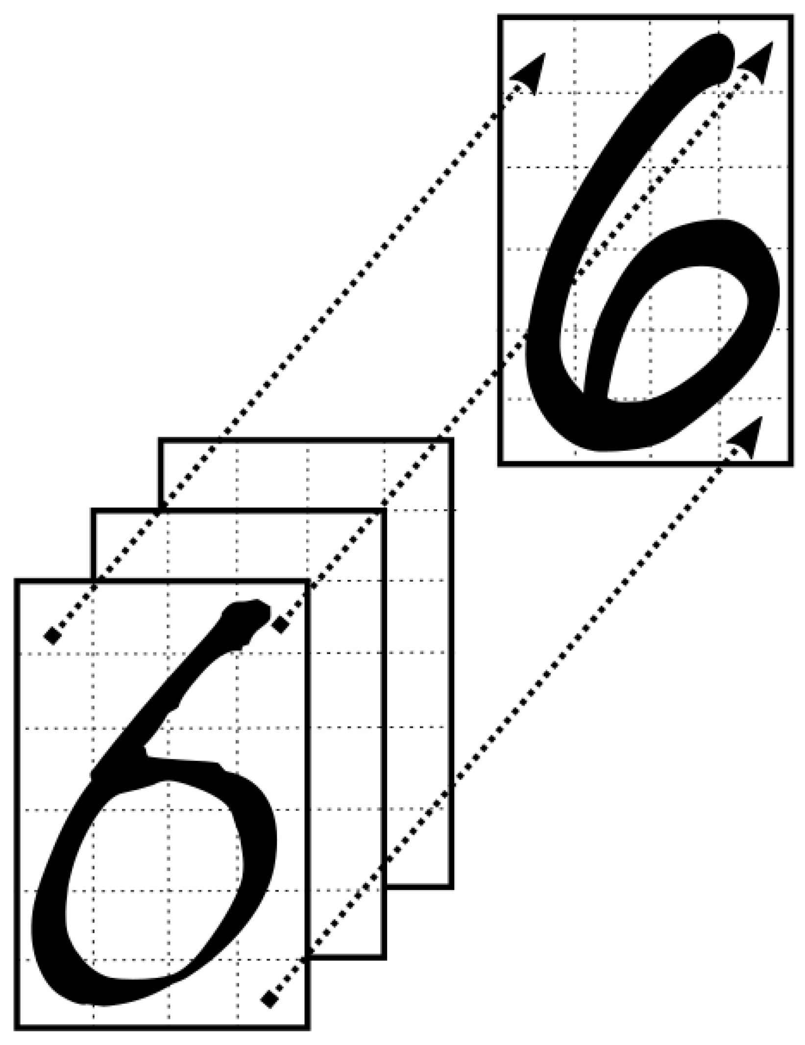
In general, H. Bremermann proposes that it can be considered that there is a universe U that contains all possible objects that can be recognized and classified. This universe is divided into different classes of objects, which are grouped under a common label (class). H. Bremermann also proposes, for simplicity, that this universe U can be represented in a plane called a retina.

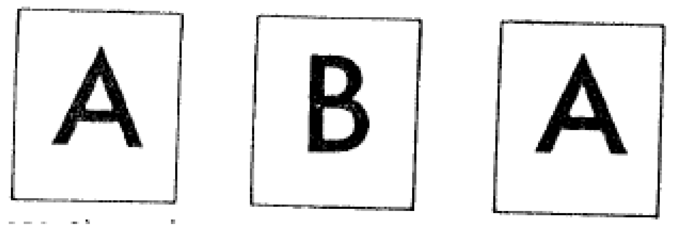
For example, in this plane (retina), handwritten characters appear individually, i.e., only a single character (at most) will appear at a time, as presented in Figure 2. In this case, our U universe would consist of all possible handwritten characters that could appear on the retina. Furthermore, if we include a class of nonsense characters, a class in which we group the possible characters that can appear on the retina that cannot be classified, our universe would include all the possible configurations that the retina can have. Since the set of possible configurations that can exist in the retina is very large, or practically infinite, it is common for practical reasons to carry out the discretization of the retina, as shown in Figure 3. Frank Rosenblat used, in his work on handwritten character recognition with perceptrons, discretization on a 20 × 20 square grid [30].

3.5. Deformable Prototypes and R. Hodges Implementation

A set of equivalent classes can be represented by individual members of those classes, and if a pattern is equivalent to a class and a set of related transformations, we can try to represent that pattern by an individual member of that class. In that case, these individual members can be called representatives of class prototypes [31].

A prototype is defined by a set of parameters ($p_i$) as follows:

$$\mathrm{Prototype} = \{p_1,\dots ,p_n\}$$

As has been shown, a prototype is represented by a series of parameters; that is, a prototype has a parametric representation. Therefore, deciding which parameters are going to define a prototype is a vital aspect; although there may be several possibilities to decide these parameters, for example, relying on expert knowledge, a first initial approach could be to carry out a feature extraction using some technique to determine these parameters. In other words, we can obtain the parametric representation of a prototype by extracting features from the set of objects belonging to the class that the prototype represents.

The main purpose of a prototype is to serve as a pattern to carry out recognition of new objects in our universe through the deformation of the prototype, that is, the deformation of the parameters that define the prototype. The prototype will be deformed until it exactly matches the new object to be recognized. For this purpose, H. Bremermann defined a matching function:

$$m_i(\mathit{x},p_1,\dots ,p_n)=\left|\mathit{x}-prototyp{e}_i(p_1,\dots ,p_n)\right|$$

(6)

where:

• $p_1,\dots ,p_n$ are the parameters that define both the prototype and the object, that is, the parameters that form the parametric representation.
• x is the new object in the universe to be recognized.
• $prototyp{e}_i$ represents each of the existing prototypes, i.e., one for each class in our U universe.

The minimum value of $m_i$ corresponds to the best match between the deformed patterns and the object that can be obtained. During the parametrization, to obtain the parameters that will define the patterns, a sufficient number of parameters must be chosen to be able to create a sufficiently large set of transformations, but it must also be in balance with the number of parameters chosen, since the smaller the number of parameters, the easier it is to use the matching function.

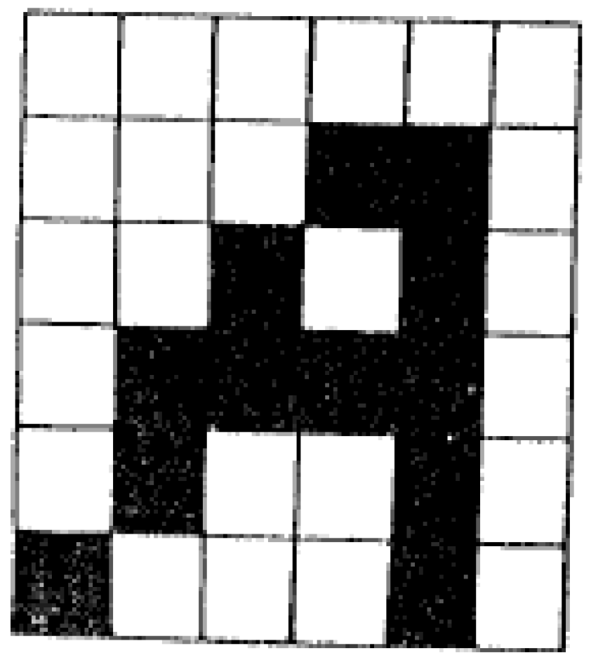
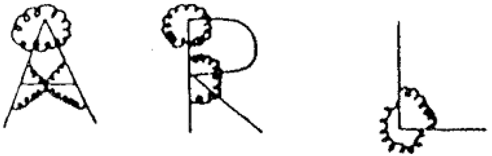
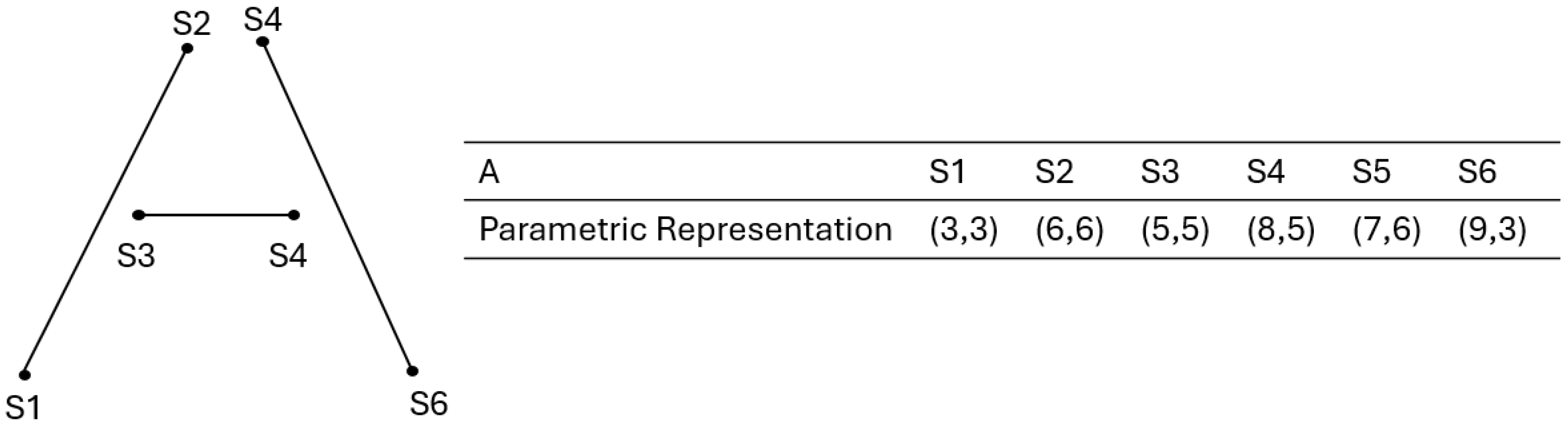
H. Bremermann believed that this matching function was not good for measuring the similarity of prototypes by itself, as some patterns can be very similar to each other and produce confusion, as shown in Figure 4, which can be a prototype of the handwritten character A or H.

Because of this, R. Hodges (a PhD student of H. Bremermann) proposed to include constraints. Hodges proposed that the prototypes should be elastic and that it was necessary to use energy to deform them; this deformation energy can be used as a measure of similarity. Hodges proposed prototypes as a set of bars and springs (later it was also proposed that a prototype could be made from a piece of an elastic matrix), as presented in Figure 5, which can be deformed by applying energy to them until they fit perfectly into an object.

R. Hodges proposed that prototypes have a fixed shape when they are in an idle state, but that they can be deformed to fit an object, although this requires energy expenditure, allowing the prototypes to be more or less rigid and better adapted to recognition. For each parametric representation, that is, for each set of parameters $p_1,\dots ,p_n$, a value of deformation energy is obtained, which is denoted as d($p_1,\dots ,p_n$); moreover, these recover their original shape when this deformation energy is no longer applied.

Combining the coincidence function proposed by H. Bremermann and deformation energy proposed by R. Hodges, they defined a function that combines the effects of both, which they called similarity function; this name should not be confused with other existing similarity functions:

$$Si{m}_i\left(x\right)=\underset{p_1,\dots ,p_n}{min}(m_i(x,p_1,\dots ,p_n)+w·d(p_1,\dots ,p_n))$$

(7)

where:

• x is the new object in the universe to be recognized.
• $p_1,\dots ,p_n$ are the parameters that define both the prototype and the object, that is, the parameters that form the parametric representation.
• $d(p_1,\dots ,p_n)$ denotes the distortion energy value by the prototype.
• w is a weighting constant; with this constant, we measure the impact of the deformation energy.
• min $p_1,\dots ,p_n$ is the minimum over all possible parameter combinations.

3.6. Fuzzy Deformable Prototypes

3.6.1. Fuzzy Prototypical Categories

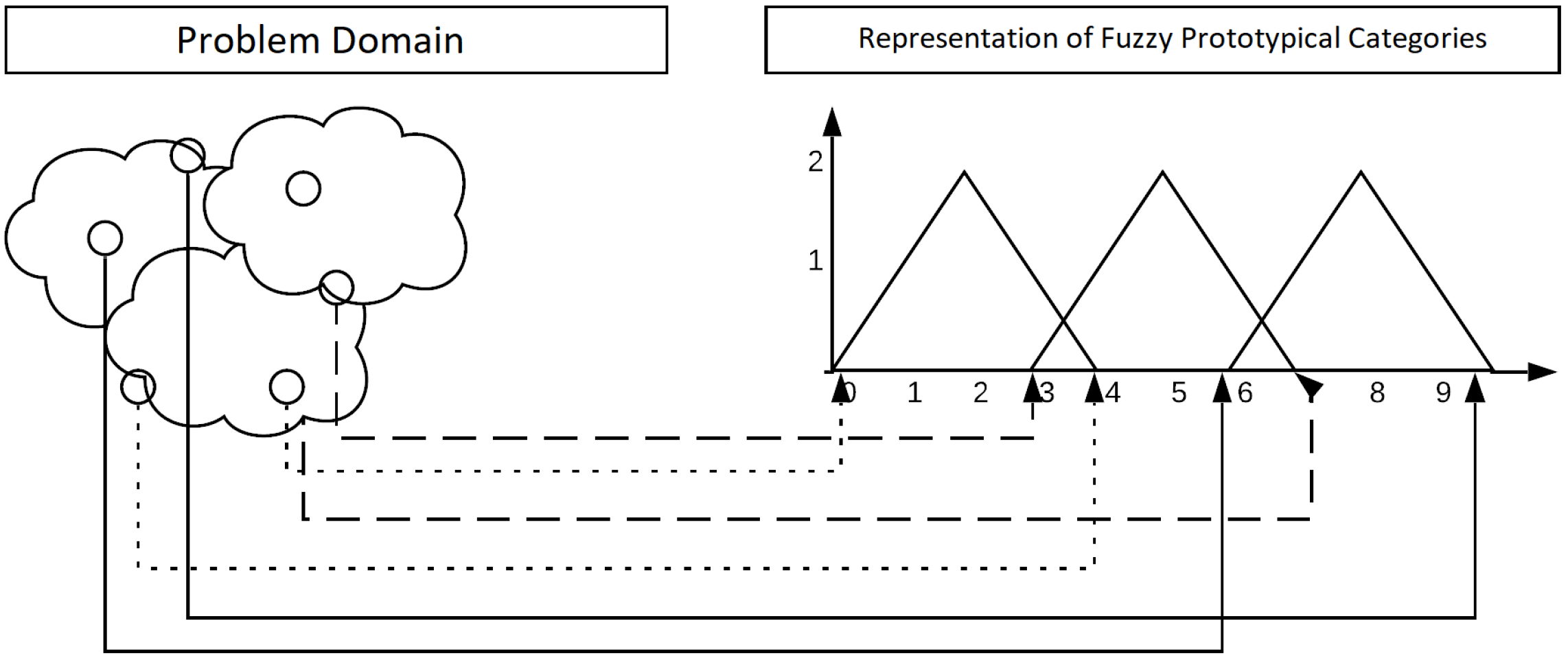
Based on previous studies in cognitive psychology and Lotfi A. Zadeh’s approach of prototypes, a new definition is given to the concept of prototype [2], which has a formal mechanism with tools from fuzzy logic. This framework is called Fuzzy Prototypical Categories [32], which inherits from psychology the characteristics listed below:

• The categories are internally structured by means of degrees of representativeness.
• The limits of the categories are not defined.
• There is a very close relationship between clusters and category structure and formation.

A graphical example of this is shown in the Figure 6.

This is formalized as follows:

• Since there is a very close relationship between attribute groups and category structure and formation, categories must be found by applying a hierarchical clustering algorithm.
• There can be as many categories as necessary to deal with the problem.
• These Conceptual Prototypes are represented by a set of terms, in which each term corresponds to a category, and this is represented by a fuzzy number.

3.6.2. Discovery of Fuzzy Prototypical Knowledge

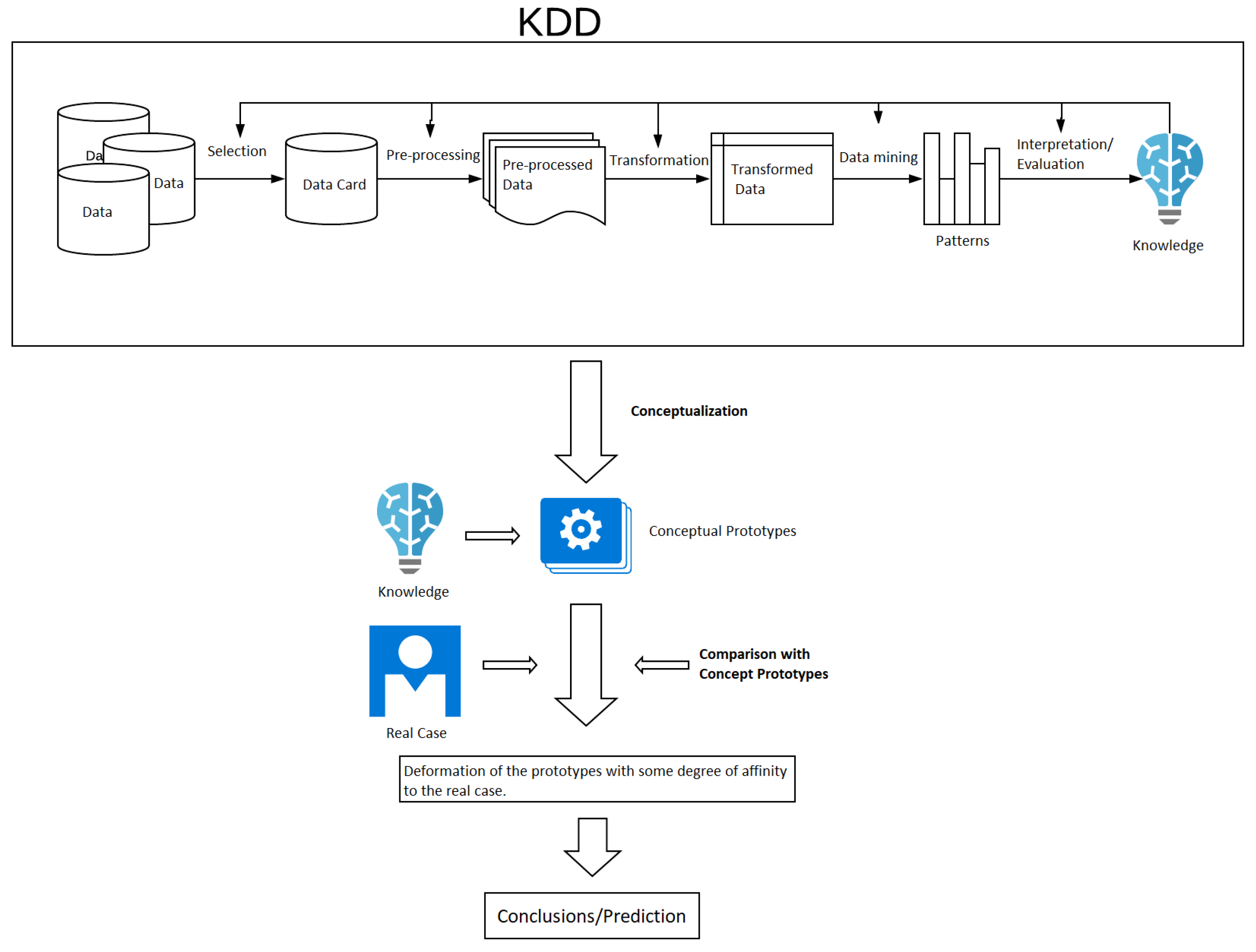
Fuzzy Prototypical Knowledge Discovery is a proposed modification of the KDD process, in which different phases with knowledge incorporation are added, where the result is ready to generate conceptual prototypes (these are based on the idea of Fuzzy Prototypical Categories) [32]. The proposed modifications to the KDD process are presented in Figure 7.

These modifications are defined as follows:

• The fuzzy model starts its development by the Data Mining phase on the available data.
• A set of contexts is defined, $A_1,\dots ,A_n$, for each one the models are generated based on Fuzzy Prototypical Categories.
• The complete model is designed taking into account the contexts $A_1,\dots ,A_n$ previously defined, inducing in each of them a collection of clusters.

This model has several advantages: its architecture is very modular since it is developed on different clusters of different contexts, and it is a very transparent model, in both execution and interpretation. Many fuzzy models focus on approximation, thus becoming black box models and losing interpretation capacity.

3.7. Prototypical Deformable Fuzzy Categories

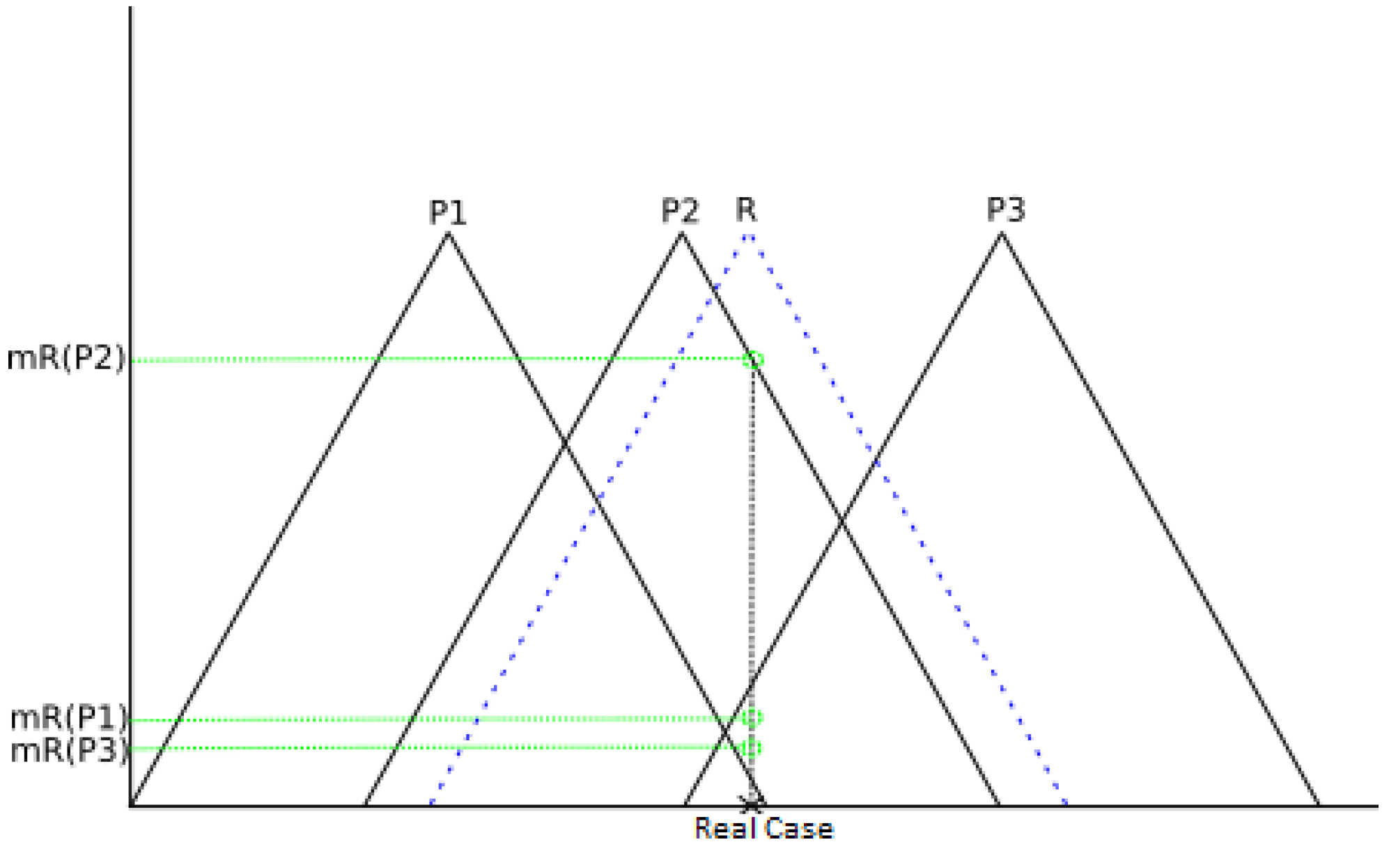
A Fuzzy Deformable Prototypical Deformable Category is a linear combination of Fuzzy Prototypical Categories with the ability to adapt to a real situation, where the coefficients are the degrees of membership of each Fuzzy Prototypical Category. In Figure 8, it is shown how this is done; a Fuzzy Deformable Prototypical Category is defined conceptually. The formal definition is shown below:

$$R.Case(w_1\dots w_2)=\mid \sum \mu p_i(v_i\dots v_n)\mid$$

(8)

where:

• R.Case: Real case.
• $(w1\dots w2)$: Parameters describing the real case.
• $\mu p_i$: Degrees of compatibility of the Fuzzy Prototypical Categories other than 0.
• $(v_i\dots v_n)$: Parameters of these Fuzzy Prototypical Categories.

Therefore, a Fuzzy Deformable Prototypical Category is a Parametric Representation in which the value of each of the parameters has been discovered through a KDD process. This new representation combines the concepts of fuzzy logic and the concept of Prototype proposed by Lofti A. Zadeh [2], including degrees of compatibility and ill-defined boundaries, Bremermann’s Proposed Deformable Prototypes, patterns with the ability to deform, and parametric representations of classes.

3.8. Elasticity

Since the proposed approach aims to simulate a physical behavior, it is important to provide an overview of relevant physical concepts, specifically in the field of Resistance of Materials, being especially interesting are the concepts of deformation and elasticity. It is therefore important to understand what happens when a force F is applied to a solid body. In general, among the possible effects that arise when a force F is applied on a solid body, the most interesting and useful ones for this work are displacement and deformation.

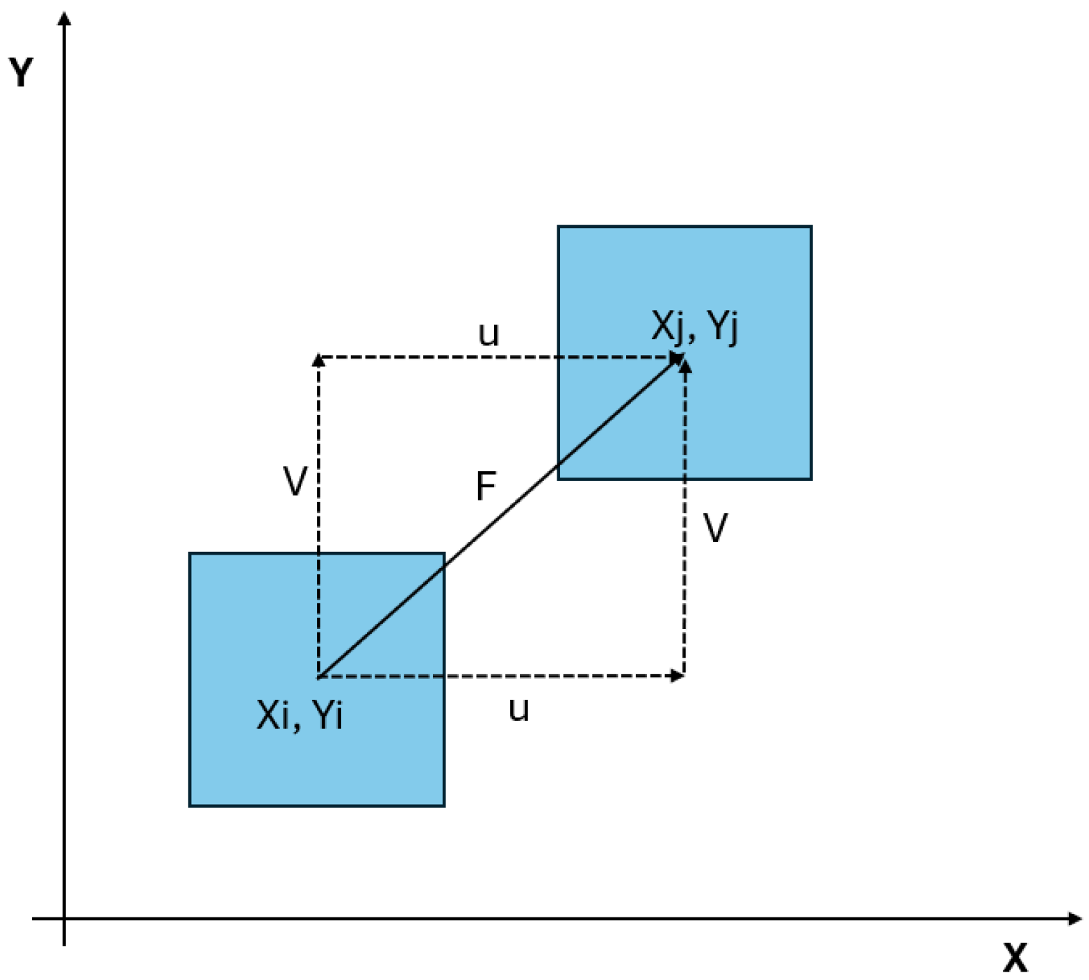
Displacement refers to the change in position of a solid body under an applied force. As illustrated in Figure 9, the body moves from an initial position $X_i,Y_i$ to a final position $X_j,Y_j$ without altering its shape. In this case, no deformation occurs [8].

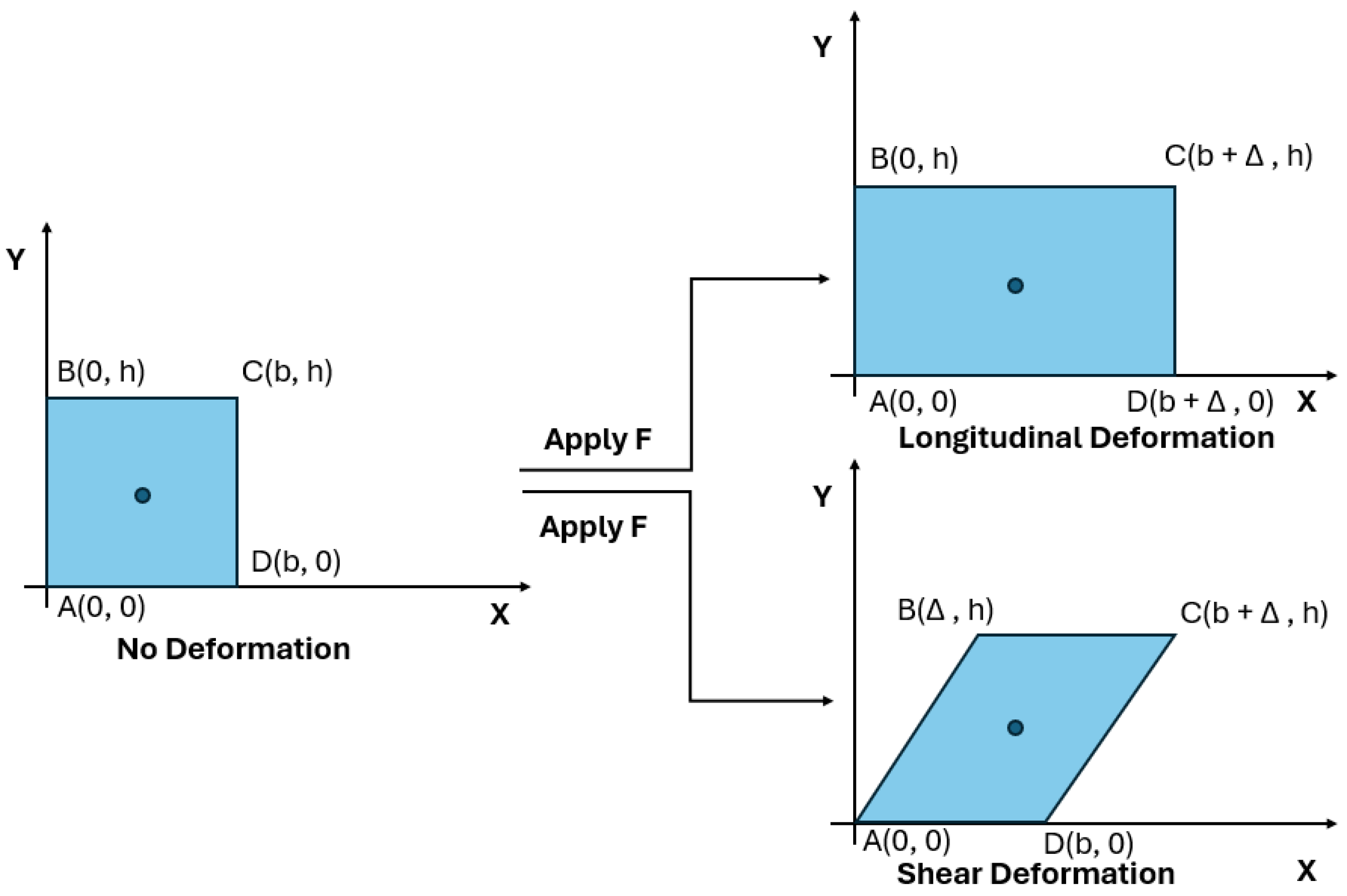
Deformation is the change, in shape or size, that a solid body undergoes when subjected to a force. In general terms, the deformations suffered by a solid body can be classified into the following categories, a graphical example of the types of deformation is shown in Figure 10:

• Longitudinal deformation. Longitudinal deformation is the deformation that produces a change in the size of a solid body due to the change in the longitudinal distance between two points after the application of force F.
• Shear deformation. Shear deformation is a deformation that produces a change in the shape of a solid body due to a change in the angle originally formed by the edges when a force is applied.

Elasticity can be defined as follows: Elasticity is the capacity of any solid object to recover its original shape after deformation caused by an applied force once the force is removed [8].

In general, we can differentiate between two types of deformation with respect to the ability of a solid object to recover its original shape after being subjected to a force and the force ceases:

• Elastic Deformation: These are the deformations of the solid object that disappear from the solid object when the force on it ceases; i.e., these deformations are temporary and are only present as long as some force is applied on the solid object.
• Plastic Deformation: These are the deformations that do not disappear from the solid object when the force on it ceases; i.e., these deformations are permanent after applying a force on the solid object.

In practice, no material is perfectly elastic; that is to say, when a force F is applied to a solid object, there will always appear a part of elastic deformation, which will disappear when ceasing F, and a part of inelastic/plastic deformations, which will remain in the solid object when ceasing F. For many materials, if the applied force does not exceed a certain threshold, permanent deformation remains negligible, and the material can be considered elastic. An example could be a steel spring. If the applied force at both ends of the spring does not exceed certain values when stretching it, it is able to recover its original form, and permanent deformations will not be appreciated in it when recovering its original form.

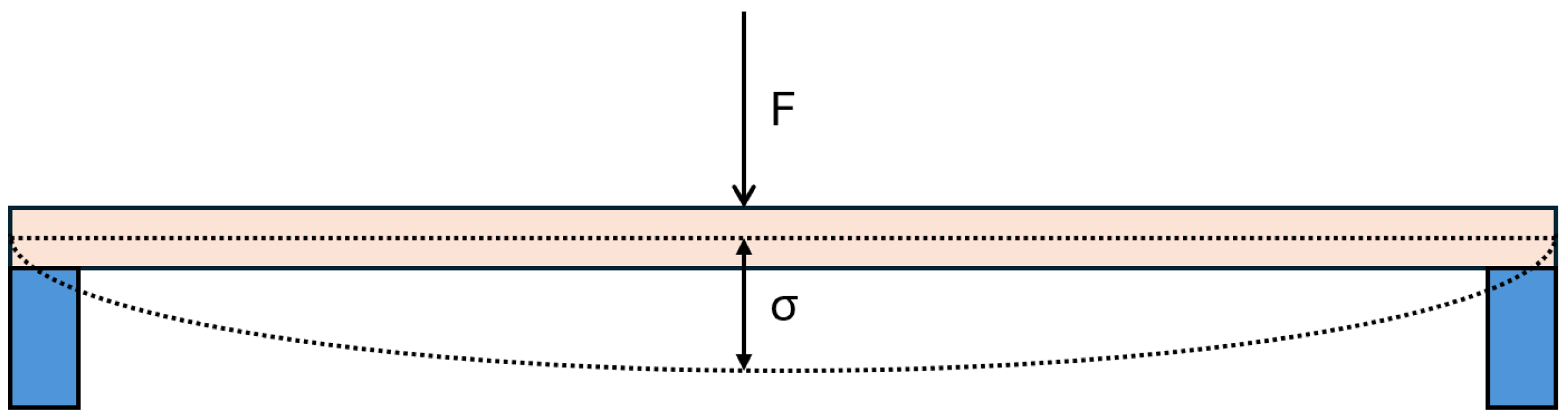
This approach of Elasticity can be understood in a simple way by means of the following experiment [8]. Consider a log of any material, for example, wood, which is resting on two supports at its extremes, such that it is elevated at a certain distance from the ground. If a force F is applied on the log, it deforms towards the ground, having a displacement $\sigma$; when the force is removed, the deformation disappears, together with the displacement $\sigma$, so the log recovers its original form. Therefore, an elastic deformation has been produced. However, if the force F exceeds a certain value, the log becomes excessively deformed, resulting in excessive displacement $\sigma$ and breaking the log, so that even if the force F ceases, the log will not recover its original shape; thus, an inelastic/plastic deformation has been produced. A graphical representation of this experiment is presented in Figure 11.

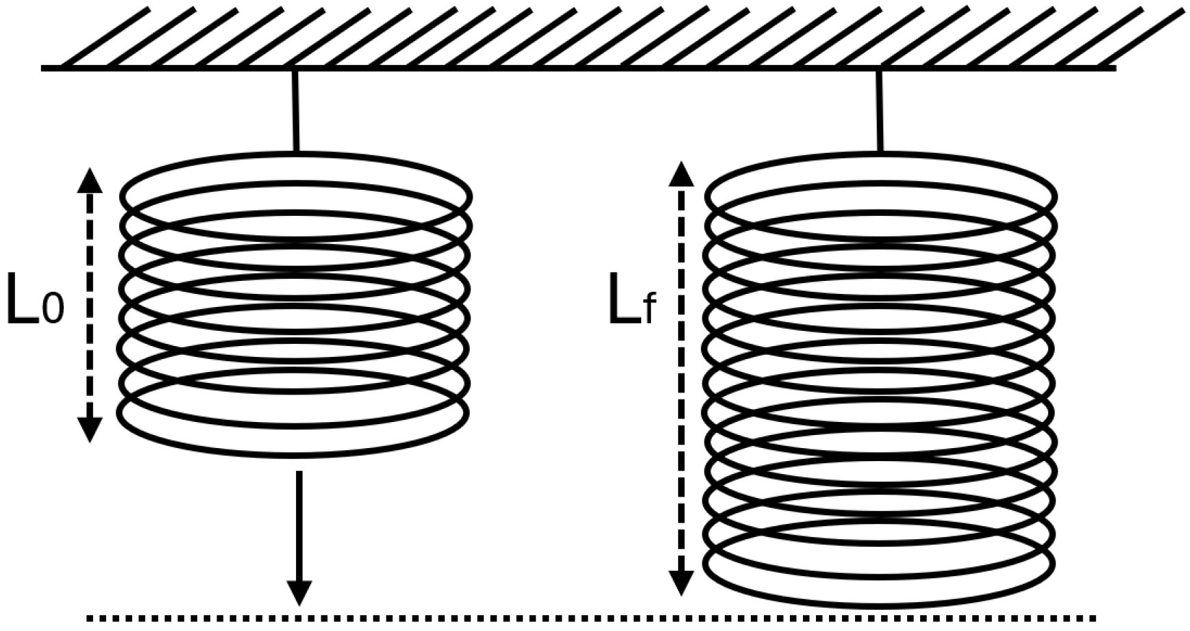
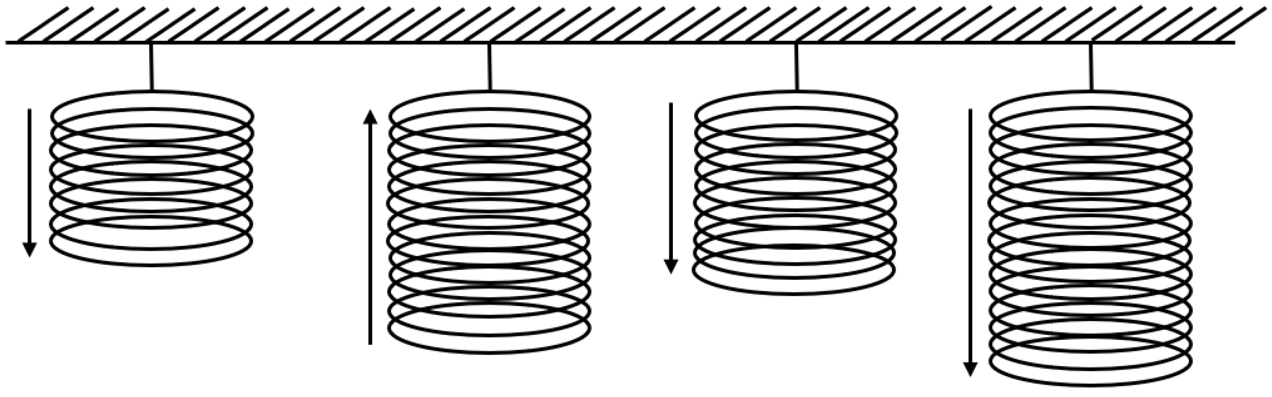
Once the basic physical approach for the behavior to be used in the proposal, such as elasticity and deformation, has been explained, it is possible to define the most important notion for this behavior. The Axial strain (also referred to as engineering strain or axial deformation) is the deformation of a solid body when a force is applied to it along a single axis. A typical example of axial deformation would be the following: Suppose that there is a solid body, for example, a spring of a material with good elastic capacity, which is fixed to a point of the ceiling at one end and a load is hung on the other, this suspended load produces a force F, which produces a deformation in the spring ($\sigma$), so the solid body has an original length (LO), and when the force F is applied, it deforms until it has a final length (LF). Figure 12 illustrates the concept of axial deformation. Given an initial value $L_0$ and a final length $L_F$, the axial deformation is defined as the relative change between these two quantities.

The axial deformation is described mathematically by the following formula:

$${\epsilon }_{i,j}={\displaystyle \frac{x_j-p_{i,j}}{p_{i,j}}}$$

(9)

where:

• $x_j$: Original length of the solid body, corresponding to $L_0$ in Figure 12.
• $p_{i,j}$: Final length of the solid body, corresponding to $L_f$ in Figure 12.

This approach provides a key advantage; it allows us to know the value of the final length of a solid body as a function of its initial length. In other words, it is possible to know how much the solid body has been deformed as a function of its original shape.

4. The Evolution to Elastic Patterns

In this section, we introduce a new framework, the EP, which will have the following bases:

• The approach of the Deformable Prototype proposed by H. Bremermann, adopting a parametric representation of the different patterns [31], which in turn is quite similar to the approach of the prototype of cognitive psychology as a central element of a category [3,4,22].
• The theoretical notion of the Fuzzy Prototype. [2] by Lotfi A. Zadeh.
• Fuzzy Deformable Prototypes, which are a combination of the previous points.

While previous works have been successful in their respective fields, Zadeh’s approach of Prototype has remained theoretical and has some limitations, for example, Fuzzy Deformable Prototypical Categories. Although these approaches effectively model real-world data, they present certain limitations. In particular, deformability is based solely on a single compatibility value, which is their degree of compatibility. So this work can be seen as an evolution of Fuzzy Deformable Prototypes.

4.1. Elastic Patterns

This new approach can be interpreted as a reformulation, recovering the Deformable Prototypes as they were conceived by H. Bremmermman and R. Hodges, but with a difference; instead of the prototype being formed by a single piece of deformable material (a spring, for example), the prototype is formed by a set of pieces of deformable material (a set of springs).

An EP can be defined as a Deformable Prototype-based representation in which each parameter is associated with an elastic component governing its adaptation to input data. From a conceptual perspective, this formulation integrates three complementary viewpoints. First, prototype theory provides the basis for representing categories through central or representative elements. Second, fuzzy logic introduces a graded notion of similarity, allowing instances to belong to a category with varying degrees. Finally, principles from physics and engineering are employed to model the deformation of the prototype as an energy-driven process.

Within this framework, classification is interpreted as the process of deforming a prototype to match an input instance, where the required deformation is quantified through an energy function. The most appropriate class is therefore identified as the one that minimizes this deformation energy. This interpretation moves beyond a purely metaphorical description and provides a mathematically grounded and physically interpretable model.

The EP can be interpreted as a higher-level model operating on top of any prototype generation mechanism. Therefore, the EP can be seen as a set of springs, which will deform independently and mimick physical spring behavior; in Figure 13, a graphical representation of the EP framework is presented. A two-level deformation is generated in order to perfectly match a new case to be characterized:

• At the parameter level (the deformation of the spring): Deforming each spring individually by means of Axial Deformation [9].
• At the pattern level (of the set of all the springs): Generating a deformation vector to introduce a general measure of deformation, the deformation energy, which will be the sum of the components of this vector.

In many classical approaches to artificial intelligence, particularly in pattern recognition, classification is performed by comparing a new instance to a set of predefined representations, such as prototypes, centroids, or stored examples. In this context, the notion of “adapting a case to existing patterns” refers to evaluating the similarity or distance between the input and these fixed structures. In contrast, the approach proposed in this work introduces a different perspective. Rather than treating patterns as static references, EPs allow prototypes to be elastically deformed in order to match the input instance. Classification is therefore interpreted as an energy-based adaptation process, where the most suitable class corresponds to the prototype requiring the least deformation. The following criterion is therefore established:

A new case is characterized by the most affine EP. The most affine EP will be the one that requires minimal energy to deform (Deformation Energy) and fits perfectly with the new case.

Since some of the fundamental aspects of this new approach are the Deformation Energy of the pattern (in order to obtain the pattern with the best match) and the deformation of each of the parameters of the pattern, obtaining these parameters, that is, the parametric representation of each of the patterns to be worked with, becomes a critical aspect, where Knowledge Engineering can be especially useful, since these patterns are going to represent classes existing in the real world.

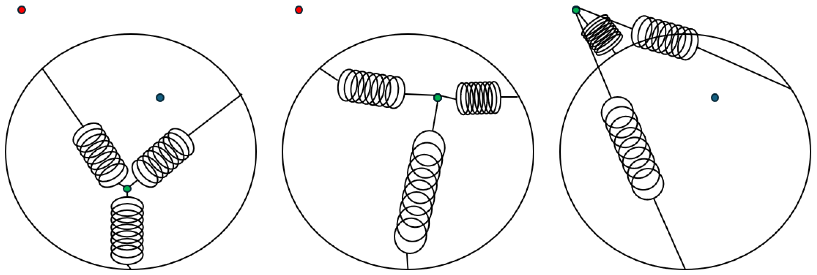
Taking up the concept of prototype from the point of view of cognitive psychology, if one conceptualizes the central element of the class, the Prototype, as a set of springs at rest (or as the constraints proposed by R. Hodges), these can be deformed to match any possible element, whether it is of the same class or not. The deformation required to exactly match an element of the same class (internal similarity) will be less than that required to exactly match an element of any other class (external dissimilarity). A graphical example of this conceptualization is shown in the Figure 14, where the black circle corresponds to a category, the blue point corresponds to elements of that category, the green point corresponds to an element to be classified, and the red point corresponds to an element of any other category. For the purpose of simplicity, in this example, the EP has three parameters, represented by three springs. Figure 14 shows three scenarios: the first in which the parameters, conceptualized as springs, are at rest; the second in which the parameters/springs are deformed to match the element to be classified with the element within the class; and the third scenario in which the springs are deformed much more than in the previous one to match the element to be classified with the element outside the class.

Therefore, this example shows how to deform the prototype, the set of springs and the first blue point, to the second blue point, a real-world object to be characterized; the energy expenditure (which we call deformation energy) is lower than that required to deform the prototype to the red point, a real-world object that does not belong to the class.

EPs offer a distinctive perspective on pattern recognition by integrating interpretability, adaptability, and a physically grounded similarity measure within a unified framework. From an interpretability standpoint, the model provides explicit insight into the classification process. Each decision is determined by the deformation required to transform a prototype into the input instance, and this transformation is quantified through an energy function. As a result, the contribution of each parameter can be directly analyzed, enabling a transparent understanding of the model behavior.

In terms of adaptability, the deformation mechanism allows the model to accommodate variations in the input data without relying on complex preprocessing or feature extraction pipelines. This property is particularly relevant in scenarios where data exhibit structural variability, as the model inherently adjusts its internal representation through controlled parameter transformations.

Regarding performance, the current implementation should be understood as a proof of concept. While it does not aim to compete with highly optimized machine learning models in terms of raw accuracy, it demonstrates that a deformation-based approach can achieve consistent and meaningful classification results. This suggests that EPs constitute a promising complementary framework, particularly in applications where interpretability and model transparency are of primary importance.

4.2. Deformation Energy Calculation

This section will give an overview of how deformation in EPs can be calculated, taking into account that, as previously explained, this deformation is carried out at two levels: the parameter level and the pattern level.

4.2.1. Calculation of Deformation Energy at Parameter Level

In order to weight the deformation at the parameter level, for each spring, it is possible to use the concept of axial deformation. This concept is commonly used to measure the deformation of a spring in a single axis, obtaining the deformation it undergoes as a function of its initial length; in other words, the deformation causes the final length of the spring to be n times the initial length [9].

This approach has a great advantage for EPs; the deformation is obtained in values relative to the spring to be deformed, not in absolute values, for example: the deformation suffered by a spring measuring 1 cm (l) and deformed by 1 cm (Δd) more is much greater than that suffered by a spring measuring 20 cm (L) and deformed by 1 cm more. In the first case, the spring would go from measuring 1 cm to measuring 2 cm (l’), which means doubling its total length, while in the second case, it would barely mean an increase in the length of the spring, which goes from measuring 20 cm to 21 cm (L’). This means that the deformations are relative to the initial measurement of the spring and, therefore, to the parameters of the prototype and the real case, so that, although the deformation in absolute values in both parameters is the same (1 cm, returning to the previous example), the relative deformation of the pattern on the real case is much greater in one parameter than in the other. The parameters that deform more individually should add more value to the total deformation when weighting the deformation energy of the pattern in the real case.

While axial deformation is defined at the parameter level, the aggregation of these local deformations gives rise to a global energy measure, which can be interpreted as a similarity criterion between the input and the prototype.

As given in Equation (1), the formula is reproduced here for clarity. The axial deformation of the parameter is defined as follows:

$${\epsilon }_{i,j}={\displaystyle \frac{x_j-p_{i,j}}{p_{i,j}}}$$

where:

• ${\epsilon }_{i,j}$: Deformation of the real-case parameter i on the prototype j, the same parameter for both.
• $x_j$: Real-case parameter.
• $p_{i,j}$: Parameter of the pattern.

Initially, $x_j$ and $p_{i,j}$ denote the real-case and prototype parameters, respectively, since conceptually they are the pattern parameters deformed to match the real-case parameter; an example of what this deformation would look like is shown below:

$$E={\displaystyle \frac{52-13}{13}}=3$$

However, this criterion may differ in real cases, as there are several possibilities not initially taken into account:

• The pattern parameter ($p_{i,j}$) can be larger than the real-case parameter ($x_j$), which raises several possible conflicting issues:

  –

  The parameter would be contracting rather than deforming/elongating. Although this was not a problem per se, the concept of axial deformation is intended to always be used with a final length greater than the initial length, which can be a contradiction conceptually.

  –

  The result of axial deformation by either elongating or contracting a parameter should be the same; however, the results differ. An example of this is given below.

  Assume that the real-case parameter has a value of 20, and the EP parameter has a value of 3; therefore, the axial deformation would be: ${\displaystyle \frac{20-3}{3}}\approx$ 5.66.

  Let us now assume that the values are reversed, the real case has a value of 3, and the EP has a value of 20; therefore, the axial deformation would be: ${\displaystyle \frac{3-20}{20}}\approx -0.85$. Deformation values are considered in absolute terms ${\displaystyle \mid \frac{3-20}{20}\mid }\approx 0.85$.

  As a first aproach, $x_j$ must always be the parameter with the largest value, whether it is the EP or the real case, and $p_{i,j}$ will be the parameter with the smallest value, regardless of whether they are the parameters of the real-world scenario or the EP; a more in-depth study of how the EP parameters can be modified could lead to new ways of adapting the EP to better suit the context.

• There is the possibility that some of the parameters, both in the EP and in the real case, have a value of zero, with the case in which $p_{i,j}$ (initially the prototype parameter) has this value being particularly conflictive. When applying the axial deformation formula, the result would be the following: ${\displaystyle \frac{20-0}{0}}\approx \infty$. This case can be interpreted as meaning that the EP must deform infinitely to coincide with the sample, which could be considered as a fracture in the EP, and this can lead to the fact that conceptually this parameter of the EP cannot be deformed, since it has a value of zero and is therefore non-existent. However, it is common for a parameter to have a value of zero, and this does not imply that the parameter is non-existent and can be deformed, but rather that this value is a label, the non-membership of a group, or that it has a semantic that indicates the absence of a characteristic. The following are several cases where this could occur, and the deformation should be able to be weighted:

  –

  In Computer Vision tools, it is very common for the encoding of a black pixel to have the value 255 and a white pixel to have the value 0, with all the possible range of greys in between these values. Therefore, the deformation of a black pixel to a white pixel is possible, even if this implies a very high deformation value.

  –

  The One-Hot Encoding technique is very commonly used to convert a categorical feature with one-hot values into numerical features. Assign a value of 0 to the new characteristic that is not the value of the original characteristic, and a 1 to the new characteristic that does represent the value of the original characteristic. An example of this would be a characteristic Colour that has the values: Blue, Red, and Green. This technique would convert this single feature (Colour) into three new style features—isBlue, isRed, and isGreen—with new columns having a value of 0 if the original record did not have the category value they represent or 1 otherwise. In this case, the value 0 has the semantics of not belonging to a class; deformation should be possible, since it would mean deforming a parameter so that this parameter changes its membership from one class to another, even if this means a penalty, which is reflected in high deformation.

  –

  Another case similar to this, where deformation should also be possible, would be a symptom vector for classifying a disease, where not all symptoms of that disease may be present, and other symptoms may be present but have little or no relation to the disease in question.

Initially this calculation of the Deformation Energy was proposed in a similar way to that used by Hopfield Networks, a type of artificial neural network in which an Energy Function is defined, which associates the state of the network to a value of energy; this energy depends on the state of the network, and as the weights of the neurons are updated, the energy decreases. However, this idea was finally discarded in favor of the previously proposed approach of using the concept of Axial Deformation, as it is conceptually closer to the representation of an EP as a set of springs.

4.2.2. Calculation of Deformation Energy at Pattern Level

The calculation of the Deformation Energy corresponds to the deformation at the level of the EP. This calculation is carried out by means of the notion of the deformation vector, which is based on the notion of the strain tensor [10]. This notion is commonly used in the mechanics of continuous media and the mechanics of deformable solids, with the aim of weighting the change in shape and volume in a body.

A deformation vector is a vector (initially one-dimensional) that represents the deformation that an EP undergoes in order to fit a real case perfectly. Each position of the deformation vector represents the deformation suffered by a specific parameter, which has been explained in the previous section on how to calculate it, so it is possible to define a deformation vector as follows:

$$\mathrm{Deformation} \mathrm{vector} = \{{\epsilon }_n,{\epsilon }_{n+1},\dots ,{\epsilon }_{n+i}\}$$

where:

• ${\epsilon }_n$: Axial deformation of the parameter n of the EP and the real case.

Finally, to calculate the Deformation Energy that an EP undergoes in a specific real case, Equation (2) is reproduced here for convenience:

$$E_i\left(x\right)={\displaystyle \sum _{j=1}^n}{\epsilon }_{i,j}$$

where:

• ${\epsilon }_{i,j}$: Each position of the deformation vector

That is to say, the Deformation Energy that a pattern undergoes to fit perfectly with a real case is the sum of each of the values of the deformation vector; that is to say, the Deformation Energy that affects the pattern is the sum of each of the individual deformations that each parameter undergoes.

4.3. Interpretability Advantage of Elastic Patterns

One of the main contributions of EPs lies not in maximizing predictive accuracy, but in providing a transparent and interpretable classification mechanism grounded in physically meaningful principles. In contrast to many contemporary ML approaches—particularly deep neural networks—which are often regarded as black-box models [33], EPs offer a fully traceable decision process.

The interpretability of EPs emerges naturally from their structural design. Each pattern is represented as a set of independent elastic components (springs), where each component corresponds to a parameter of the underlying representation. When a new instance is evaluated, the model computes the deformation required for each parameter, quantified through axial strain, and aggregates these into a global deformation energy. The classification decision is then obtained by selecting the pattern that minimizes this energy.

This process provides interpretability at two complementary levels:

• Parameter-level interpretability: Each parameter contributes independently to the final decision through its associated deformation. This allows practitioners to identify which features require the greatest adjustment, offering a direct explanation of why a particular classification is made.
• Global interpretability through energy minimization: The total deformation energy acts as a physically grounded similarity measure. Unlike abstract distance metrics, this energy has an intuitive interpretation: it quantifies the effort required to adapt a known pattern to a new instance. This aligns with the principle that similar instances require less transformation, providing a natural and interpretable decision criterion.

This dual-level interpretability distinguishes EPs from traditional prototype-based methods. While classical approaches such as KNN or centroid-based models provide some degree of transparency, they do not explicitly model the process of adaptation between instances. In contrast, EPs explicitly simulate this adaptation through deformation, making the reasoning process observable and quantifiable.

Furthermore, the proposed framework aligns with the growing body of research advocating for inherently interpretable models rather than post hoc explanations [33]. Unlike model-agnostic explanation techniques such as LIME [34] or SHAP [35], which approximate the behavior of complex models, EPs are interpretable by design. This eliminates the need for secondary explanation layers and avoids potential inconsistencies between the model and its explanations.

From a conceptual standpoint, the use of physically inspired principles—such as elasticity and energy minimization—provides an additional layer of interpretability. Physics-based analogies have been shown to facilitate human understanding of complex systems by grounding abstract computations in familiar mechanisms [36]. In this context, the deformation of springs offers an intuitive visual and conceptual metaphor for classification, making the model particularly suitable for domains where explainability is essential.

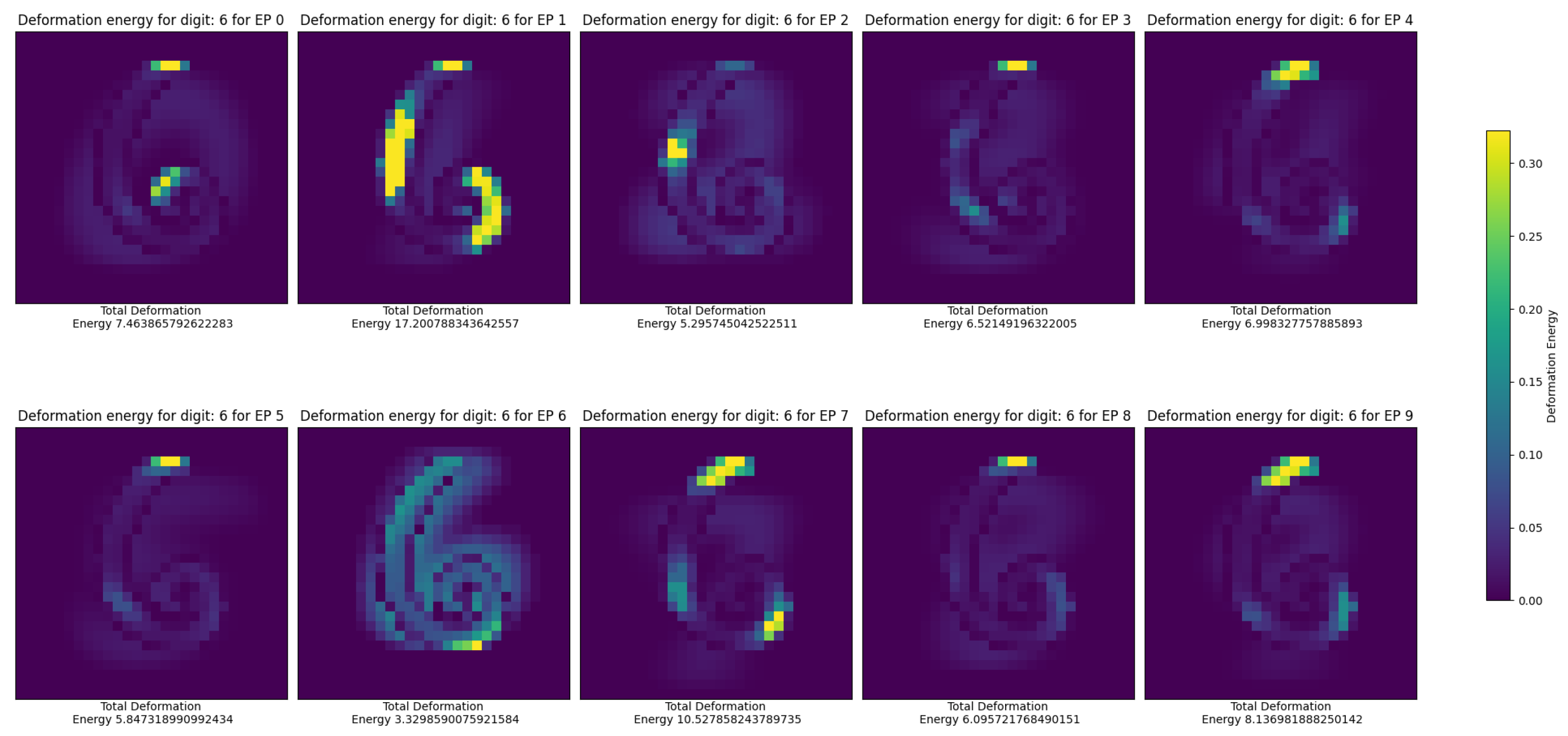
Figure 15 illustrates the deformation energy associated with each EP corresponding to the digits 0–9 when applied to an input sample representing the digit 6. This example is discussed in detail in Section 5. Each heatmap visualizes the spatial distribution of deformation energy, where lower values indicate regions of strong correspondence between the prototype and the input, and higher values reflect areas requiring greater adaptation. This representation provides an explicit and interpretable view of the matching process, as the classification decision emerges from the global energy minimization while remaining locally traceable. In this sense, the model offers ante hoc interpretability, as both the decision and its underlying rationale can be directly examined through the energy distribution, without the need for post hoc explanation mechanisms.

In summary, EPs should be understood as an interpretable, physics-inspired classification framework in which decisions are not only computed but also explained through their underlying mechanism. This positions the approach as a valuable alternative in scenarios where transparency, traceability, and conceptual clarity are prioritized over raw predictive performance.

4.4. Prototype Generation Strategy

In the present work, the generation of initial prototypes is intentionally kept simple in order to isolate and evaluate the contribution of the elastic deformation mechanism. Prototypes are constructed directly from the available data without employing advanced clustering or fuzzy modeling techniques.

It is important to note that the EP framework is inherently modular with respect to prototype construction. The deformation-based classification mechanism does not depend on a specific method for generating prototypes, and therefore, more sophisticated approaches can be incorporated without altering the core formulation.

In particular, methods based on fuzzy clustering, such as FCM, provide a natural extension of the proposed framework. These approaches would allow prototypes to be defined as fuzzy representatives of data distributions, thereby aligning more closely with the theoretical foundations derived from fuzzy set theory and cognitive prototype models.

5. A Case of Use: OCR with Elastic Patterns

5.1. MNIST Dataset

In order to study the viability of the EP, a preliminary experiment is proposed. MNIST is one of the most widely used datasets to carry out classification and artificial intelligence tasks due to the large set of classified and varied samples available. It has been widely used in numerous studies [37,38].

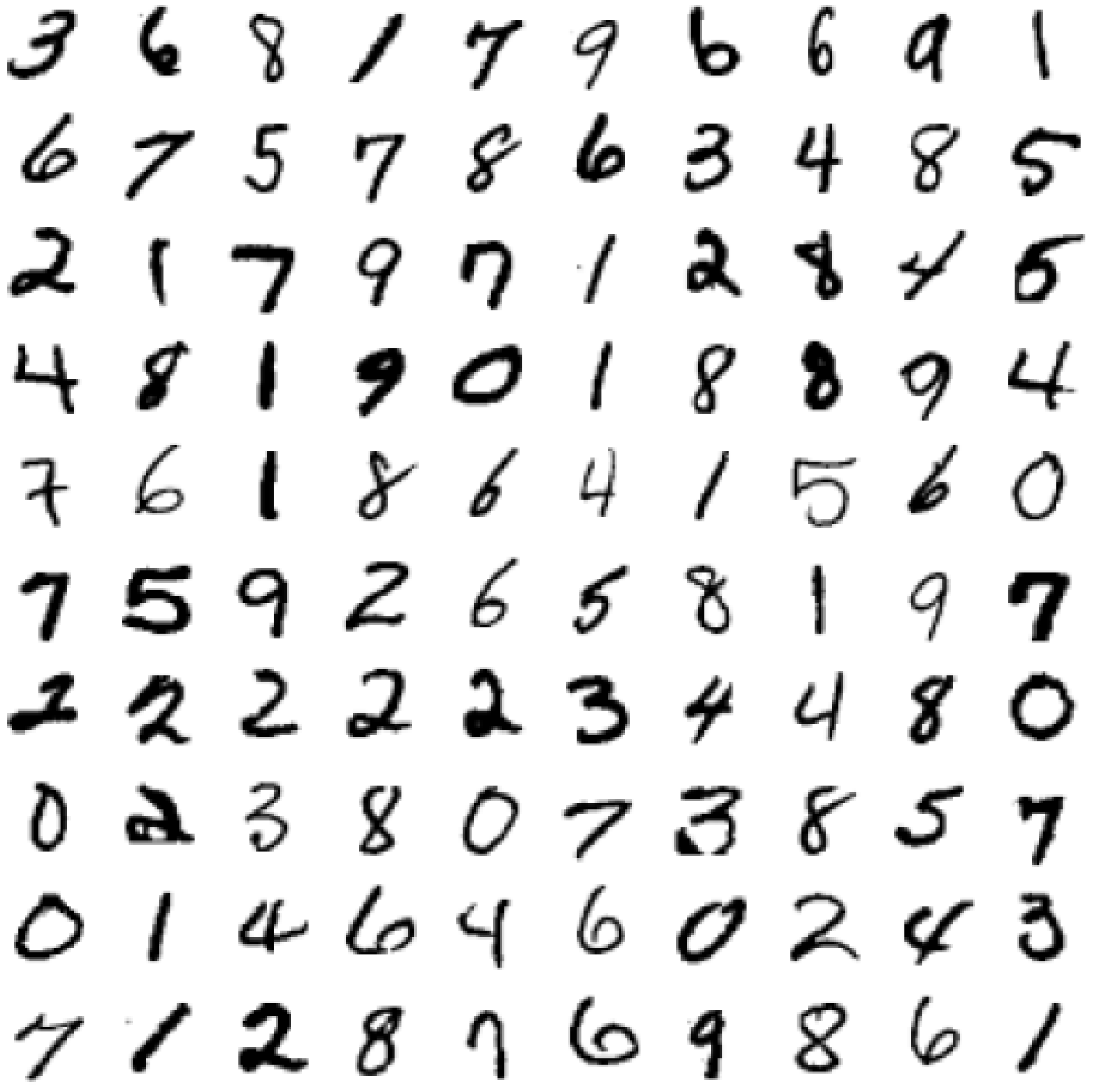
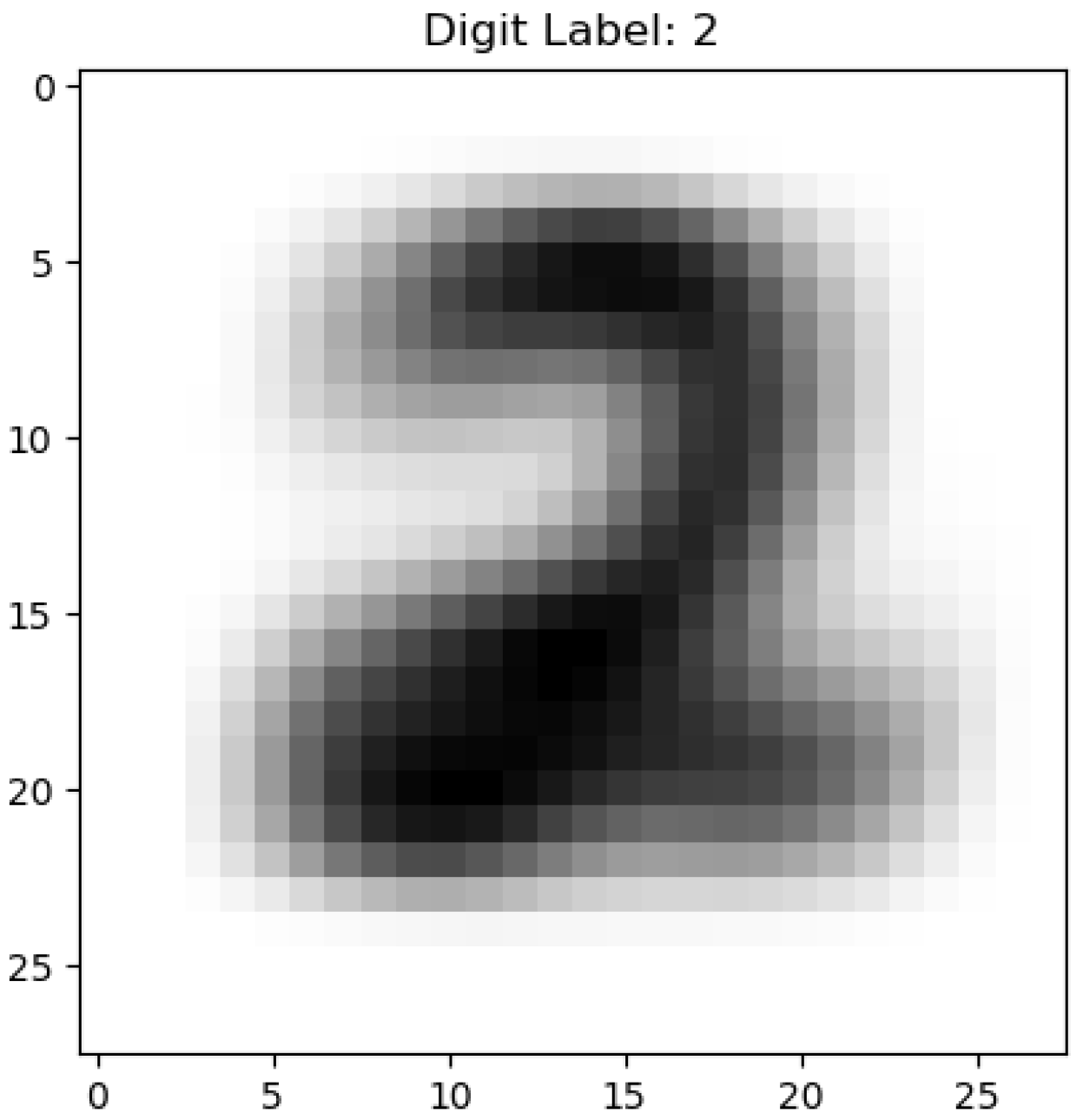
This database arises from a proposed modification of the NIST database, focusing especially on the Special Database 3 (SD-3) and Special Database 1 (SD-1) sets, which collect binary samples of handwritten data. NIST was originally designed to use the SD-3 set as the training set because this set is much cleaner and easier to use, and the SD-1 set is used as the test set. This is mainly because the set SD-3 was generated by collecting samples among workers of the US Census Bureau, while the set SD-1 was generated by collecting samples among students at different institutes [39]. Mixing the two sets resulted in a new set NITS–Modified (MNIST). An example of the available MNIST samples is shown in Figure 16.

It is important to note that the MNIST dataset is inherently pre-processed, including centring, normalization, and noise reduction. Therefore, the present evaluation does not fully reflect the behavior of EPs under raw input conditions. It is worth noting that MNIST is widely regarded as a relatively simple benchmark dataset. In this work, it is therefore used as a proof of concept to illustrate the feasibility of the EP framework. In order to assess the generality of the approach, additional experiments on datasets of different natures and complexities are considered.

5.2. Elastic Pattern Generation

As mentioned above, the generation of EPs is a fundamental aspect in the proposed classification method; however, the way to generate these EPs may be different depending on the problem and the context we are working with. In general, as in other works [32], as many EPs are generated as there are class labels in the context. As previously proposed, one fundamental aspect of the EP framework is the notion of parametric representation, that is, how an object (or prototype in this context) is represented by a set of sufficient parameters to be able to represent it and its related transformations. In Figure 17, an example of parametric representation is presented, based on the approach of H. Bremermann, defining a prototype of the character A as three lines in space, or six points. So, as a result, we can convert the prototype of the character A proposed by H. Brememann, which would have a parametric representation as a vector of six parameters: the endpoints of the three lines forming the character.

The context we are working with in this case, the MNIST database, has 10 possible values or categories, the digits from 0 to 9, so there will be 10 possible EPs, each of them representing a value or category, a digit in this context. In the following, we will show how to generate the EP necessary to classify new samples with the MNIST subset described above.

To generate the EP, it is possible to rely on the approach of mask [31]. Conceptually, these EPs are understood as a matrix of the same dimensions as the samples used in the training set, in which each position has a value in the range [0–255], with the value 0 being commonly understood as a white pixel and the value 255 a black pixel. Each position in this matrix, one pixel in particular, represents how common it is that in each of the samples, this pixel appears darkened; in other words, that in the sample, this pixel has been written on. For this purpose, a small algorithm is defined for the generation of each of the patterns:

1.

Select from the set of samples of the training set all the samples that share the same class, for example, all the samples that represent the digit 1 in this case.

2.

Generate a matrix of the same dimensions as each sample of the training set; this matrix will have all its positions with value 0, and this matrix will finally be the EP.

3.

An increment is calculated with the following formula:

$$\mathrm{increment} = 255/\mathrm{Number} \mathrm{of} \mathrm{samples} \mathrm{in} \mathrm{the} \mathrm{training} \mathrm{set}.$$

For this case, the value of the increment is:

$$\mathrm{increment} =255/\mathrm{60,000} = 0.00425.$$

4.

Scroll pixel by pixel through each of the previously selected samples; if this pixel has a value other than 0—that is, it is not a blank pixel and greater than a certain threshold U—this represents the user’s intentionality to write on that pixel. As a first approach, the U threshold was set to 80. The previously calculated increment value is added to the pixel corresponding to the EP.

5.

Finally, the obtained EP is checked pixel by pixel, rounding its value to an integer value, since, as previously explained, all pixel values will be in the range [0–255].

A graphical representation of the proposed method is shown in Figure 18. An example of how the obtained EP would be graphically represented is shown in Figure 19.

5.3. Elastic Pattern Recognition

Once the different EPs, which represent the digits from 0 to 9, have been generated, following the method proposed in the previous section, it is possible to make use of them to carry out characterization/recognition of new samples. During the recognition phase, each input instance is compared against the set of elastic prototypes by computing the deformation energy required for adaptation. The instance is then assigned to the class associated with the prototype that minimizes this energy.

One practical advantage of the proposed approach is that it does not require additional task-specific preprocessing or feature extraction beyond the standard representation of the data. In the case of the MNIST dataset, the input images are already normalized and structured, and the method operates directly on this representation. In contrast to many conventional approaches, which rely on carefully designed preprocessing pipelines to enhance feature extraction or reduce variability, the EP framework models variability through deformation of the prototype itself. As a result, the need for explicit preprocessing steps is reduced, as variations in the input are handled within the model through the deformation mechanism. This property should not be interpreted as the complete absence of preprocessing, but rather as a reduced dependence on explicit transformation pipelines.

In this case, and as previously proposed, there is the possibility that when calculating the axial deformation, that is, the deformation at the parameter level, some of the parameters have a value of 0, which does not mean that the parameter is non-existent, but rather that this value of 0 is a label. The value 0 for a parameter indicates that we are working with a white pixel; therefore, the deformation must be possible, and it must be possible to calculate it. However, applying the axial deformation formula with any of the parameters having a 0 value could be a problem, so in this case, if any of the parameters have such a value, it would be replaced by the 1 value; this represents a very small deformation over the total range of values that the parameter can take.

The proposed method for making use of the previously generated EP, and characterization/recognition of the test set samples is similar to that commonly used for recognition using masks:

1.

For each EP of those previously generated, obtain its deformation vector; to do so, calculate the deformation vector for each EP–sample pair to be recognized.

2.

Iterate parameter by parameter (pixel by pixel in this case) in parallel with the EP and the sample to be recognized, obtaining the axial deformation, in other words, the deformation at the parameter level, and adding that energy value to the deformation vector.

3.

Calculate the deformation energy of each EP based on its deformation vector.

4.

Given the energy consumed by each EP to perfectly match the sample to be recognized/characterized, the sample that requires the least deformation energy is the most affine, and therefore, the sample will be classified/recognized with the class of the most affine EP.

This formulation allows the classification process to be interpreted in terms of explicit transformations, where the contribution of each parameter to the final decision can be directly analyzed.

5.4. An Example of Using Elastic Patterns with MNIST

The following is an example of how to use EPs for the MNIST sample recognition use case; however, for simplicity, only four parameters (pixels) of the EP and one sample for recognition will be shown, since both have 78 parameters (pixels), and the performance of the proposed method is independent of the number of parameters. The data of this example are shown in

Table 2. Parameters (pixels) of the EP and of the sample to be classified.

	${\mathit{P}}_1$	${\mathit{P}}_2$	${\mathit{P}}_3$	${\mathit{P}}_4$
Sample	165	180	175	154
$P{E}_0$	0	32	52	46
$P{E}_1$	178	180	200	210
$P{E}_2$	75	45	65	72
$P{E}_3$	83	94	54	62
$P{E}_4$	120	124	132	142
$P{E}_5$	0	10	12	8
$P{E}_6$	90	110	122	112
$P{E}_7$	64	20	52	47
$P{E}_8$	64	20	52	47
$P{E}_9$	84	78	52	64

and

Table 3. Axial deformations of the parameters (pixels) and deformation energy of the patterns, with the results truncated to two decimal places.

	${\mathit{P}}_1$	${\mathit{P}}_2$	${\mathit{P}}_3$	${\mathit{P}}_4$	Deformation Energy
$P{E}_0$	164	4.62	3.84	2.34	174.8
$P{E}_1$	0.07	0	0.14	0.36	0.57
$P{E}_2$	1.2	3	1.69	1.13	7.02
$P{E}_3$	0.98	0.91	2.24	1.48	5.61
$P{E}_4$	0.37	0.45	0.32	0.08	1.22
$P{E}_5$	164	17	13.58	18.25	212.83
$P{E}_6$	0.83	0.63	0.43	0.37	2.26
$P{E}_7$	0.33	0.28	0.30	0.64	1.55
$P{E}_8$	1.57	8	2.36	2.27	14.2
$P{E}_9$	0.96	1.30	2.36	1.40	6.02

, including the calculation of the deformation vectors and the deformation energy of each pattern.

In Table 3, each of the rows obtained represents the deformation vector obtained for an EP and its deformation energy. As can be seen in the results obtained, the most affine EP is the one corresponding to the digit 1 (being able to classify the sample as a digit 1). We can also see how digits with a very different morphology, such as the digits 0 and 5, obtain a high deformation energy, and digits with a similar morphology, such as the digits 4 and 7, obtain a much lower deformation energy.

6. Application to Structured Data: Wisconsin Breast Cancer Dataset

In order to evaluate the generality of the EP framework beyond image-based data, an additional experiment has been conducted on a structured dataset. Unlike image classification tasks such as MNIST, where data are represented as spatial grids, structured datasets consist of feature vectors describing measurable properties. This experiment aims to demonstrate that EP can be naturally extended to this type of data without requiring modifications to the underlying deformation-based classification mechanism.

The dataset selected for this purpose is the Wisconsin Breast Cancer dataset, which is widely used as a benchmark in classification tasks involving medical diagnostic data. It consists of instances described by a set of numerical features extracted from digitized images of fine needle aspirates of breast masses. These features characterize properties such as radius, texture, perimeter, area, and smoothness, among others. Each instance is labelled as either benign or malignant, resulting in a binary classification problem with moderately high dimensionality.

To construct the EP, the dataset is first divided into two disjoint subsets: a training set and a test set. The training set is used to generate the parametric representation of each class, while the test set is employed for evaluation purposes. The generation of EPs is carried out through a simple aggregation strategy applied to the training data. For each conceptual class—a malignant sample or a benign sample—a grouping function is used to obtain a representative prototype. As a first implementation, this grouping function is defined as the arithmetic mean of each feature value across all training instances belonging to the same class. As a result, each class is represented by a vector of mean values, where each component corresponds to a parameter of the EP. The simplicity of the aggregation function allows isolating the effect of the deformation mechanism, while more sophisticated approaches (for example, fuzzy clustering) may further enhance the representational capacity of the model.

Once the EPs have been defined, the recognition process follows the same principles described for the MNIST case. Given a new instance from the test set, the model computes the deformation required for each parameter in order to match the instance to each class/EP. This deformation is quantified using the axial deformation measure, and the corresponding deformation energy is calculated at the pattern level by aggregating the contributions of all parameters.

The classification decision is then obtained by assigning the instance to the class whose EP requires the least deformation energy to adapt to the input. In this way, classification is interpreted as an energy minimization process, where the most compatible pattern is the one that undergoes the smallest transformation.

The results obtained in this experiment indicate that EPs can be successfully applied to structured numerical data, maintaining the interpretability and physical grounding of the model. Specifically, an accuracy of 91.48% has been achieved on the test set, demonstrating the feasibility of the approach in a non-image context. Although further improvements in prototype generation and parameter tuning may enhance performance, these results support the claim that the EP framework is not limited to image-based representations.

This experiment highlights the flexibility of the proposed method, showing that each feature of the dataset can be directly associated with an independent elastic component. Consequently, the deformation process provides a meaningful interpretation of how each feature contributes to the classification decision, reinforcing the interpretability of the model in practical applications.

7. Evaluation

7.1. For OCR with Elastic Patterns

After performing the generation of the EP and characterization/recognition of the set of test samples, the results obtained are presented; these may vary slightly from one run to another due to the fact that the training and test sets are created randomly, and therefore, from one run to another, the samples that form both sets change, although the results are very similar:

• The generation time of the EP is approximately 20 s.
• The correct classification rate is approximately 80 %; out of 10,000 samples in the test set, 8067 samples are correctly recognized.
• The run time is approximately 90 s.

In addition, a confusion matrix is obtained to see which digits are most confused when performing the classification, which is set out in

Table 4. Confusion matrix of the results obtained. The columns correspond to the assigned class and the rows to the actual class.

	0	1	2	3	4	5	6	7	8	9
0	952	0	7	4	1	4	6	0	67	0
1	0	983	23	12	1	30	8	1	57	1
2	20	2	804	12	6	0	48	6	57	3
3	13	6	71	767	1	16	9	9	64	39
4	6	1	30	4	713	9	20	4	55	136
5	41	4	12	125	14	558	20	3	68	23
6	18	10	27	0	3	27	875	0	19	1
7	19	10	14	4	27	2	1	774	49	99
8	12	21	27	63	7	21	5	1	823	39
9	28	1	11	8	83	7	1	29	60	818

.

Some conclusions can be drawn from this confusion matrix:

• The main diagonal, which represents the successes, has high values, so the percentage of successes is high.
• The digits with the highest number of hits are 0 and 1, with the digit with the lowest number of hits being 5, and then (with a fairly wide difference) 4 and 3. This is due to the fact that the numbers with the highest number of hits (0 and 1) have a less similar morphology (and therefore are less confusable) to the rest of digits, while the digits with a similar morphology to the rest of digits (5) are more easily deformed into these and therefore more easily confusable. For example, the digit 0 can be easily deformed (and therefore confused) into the digit 8 (as can be seen in the confusion matrix), while the digit 5 can be easily deformed (and therefore confused) with a larger number of digits, such as the digits 3, 6, 8, 9.
• Digits with a significantly different morphology would therefore require a large deformation of the EP and have a low number of failures in their classification. For example, no digit has ever been assigned as the digit 0 to a sample of the digit 1, as the digit 2 to a sample of the digit 5, or as the digit 7 to a sample of the digit 6.
• In this case, we are working with data prone to errors: user input errors, errors caused by malfunctioning of the writing instruments (causing ink smudging, for example), scanning errors, etc. For example, each person will have a different style of writing digits, so two samples of the same digit may differ a lot from each other, or even the opposite may be the case; two samples of different digits from two different people may be very similar to each other. Therefore, the higher the quality of the data in the training set (clearer samples, greater diversity, better processed, without typing errors, etc.), the higher the quality of the EP, which has a direct impact on their better performance.

In addition, the same test is carried out but using other widely tested and used classification methods; the results obtained are shown in

Table 5. Comparison of the results of the experiment with other common methods.

	Elastic Patterns	Random Forests	Adaboost	KNN
Success rate (%)	81.19%	63.62%	74.18 %	97.54%
Execution time (seconds)	80.49	103.03	176.22	734.87

.

7.2. Application to Structured Data

After performing the generation of the EP and characterization/recognition of the set of test samples, the results obtained are presented; these may vary slightly from one run to another, due to the fact that the training and test sets are created randomly, and therefore, from one run to another, the samples that form both sets change, although the results are very similar:

• The generation time of the EP is approximately 0.5 s.
• The correct classification rate is approximately 91 %; out of 188 samples in the test set, 172 samples are correctly recognized.
• The run time is approximately 0.5 s.

The results show that the choice of feature set and clustering function has a significant impact on the method’s performance. In particular, the use of features corresponding to mean and worst values, together with a group function based on the mean, yields the best result, achieving an accuracy rate of 91.48%. This result suggests that combining information on the mean and worst values of morphological characteristics may be particularly relevant for detecting patterns associated with malignant cells. This may be because, when classifying a cell as malignant, highly irregular morphology is a possible indicator.

A confusion matrix is obtained to see which digits are most confused when performing the classification, which is set out in

Table 6. Confusion matrix of the results obtained. The columns correspond to the assigned class and the rows to the actual class.

	Benign	Malignant
Benign	110	1
Malignant	15	62

.

In addition, the same test is carried out but using other widely tested and used classification methods; the results obtained are shown in

Table 7. Comparison of the results of the experiment with other common methods.

	Elastic Patterns	Random Forests	Adaboost	KNN
Success rate (%)	91.48%	87.97%	89.04%	96.54 %
Execution time (seconds)	0.6	0.7	0.5	6.74

:

The results obtained across different datasets suggest that EPs can be applied to heterogeneous data types, including both structured numerical data and image-based representations. However, performance tends to decrease as data complexity increases, indicating that further refinement of the prototype generation and deformation mechanisms is required to improve scalability.

8. Conclusions and Future Work

8.1. Conclusions

This work has introduced EPs as a novel classification framework that combines prototype-based reasoning, fuzzy representations, and physically inspired deformation mechanisms. The proposed approach departs from conventional classification paradigms by modeling patterns as collections of elastic components, enabling the adaptation of class representations to new instances through controlled deformation. The proposed framework demonstrates that it is possible to combine interpretability and adaptability within a physically grounded classification model. Although further optimization is required to improve performance, the results indicate that EPs represent a promising alternative for applications where transparency and conceptual clarity are essential.

A key contribution of this research is the explicit integration of interpretability into the core of the model. Unlike many contemporary ML approaches, where decision processes are often opaque, EPs provide a fully transparent mechanism in which each classification outcome can be understood in terms of parameter-level deformations and the associated deformation energy. This dual-level interpretability offers both local and global insight into the reasoning process, facilitating analysis, validation, and potential expert interaction.

The experimental evaluation on the MNIST dataset has demonstrated the feasibility of the approach as a proof of concept. Although the predictive accuracy is lower than that of established methods such as KNN or modern deep learning architectures, this result should be interpreted in the context of the model’s primary objective: to provide a physically grounded and interpretable classification mechanism rather than to optimize performance on benchmark datasets.

The evaluation on multiple datasets highlights both the flexibility of the EP framework and its current limitations when dealing with more complex data distributions. This reinforces the need for further research aimed at improving scalability and robustness.

A limitation of the present study is that the evaluation has been conducted on a pre-processed dataset. Future work should consider the application of EPs to raw and unstructured data in order to further validate their robustness to input variability.

A limitation of the current implementation is the use of a simplified prototype generation strategy, which does not fully exploit the concepts of fuzzy membership or cognitive clustering discussed in the theoretical background. While this choice allows for a clearer evaluation of the deformation mechanism, it introduces a gap between the theoretical foundation and the practical implementation. Bridging this gap constitutes an important direction for future research. In particular, the integration of fuzzy clustering techniques, such as FCM, would enable the construction of prototypes that better capture the internal structure of the data, potentially improving both interpretability and classification performance.

From a methodological perspective, EPs open a new line of research at the intersection of prototype theory, fuzzy systems, and physics-inspired modeling. The formulation based on deformation energy provides an intuitive and extensible framework that may be further refined through improved parameter estimation, alternative energy formulations, or hybridization with data-driven techniques.

In summary, EPs should be understood not as a competitor to state-of-the-art black-box models in terms of raw accuracy, but as an interpretable and conceptually grounded alternative that provides meaningful insight into the classification process.

8.2. Future Work

Future work will focus on enhancing the scalability and accuracy of the approach, exploring its application to more complex datasets, and investigating its integration with learning mechanisms that preserve interpretability. In addition, the explicit representation of deformation processes offers potential for visualization and human-in-the-loop systems, reinforcing the suitability of EPs for domains where explainability is a critical requirement. In addition, the explicit representation of deformation processes offers potential for visualisation and human-in-the-loop systems, reinforcing the suitability of EP for domains where explainability is a critical requirement. In addition, comprehensive study on how EP deforms and improve the functioning of the EP, its can be divided mainly into two distinct areas of work:

• A comprehensive study on how the deformation of the EP is carried out to fit the real case to be classified, with several possible purposes in this aspect: study how the deformation is produced at the parameter level, attempting to propose new possible deformation models for the EP, study how it is possible to work with problematic values, etc.
• Use the EP in a complex system within a cognitive environment to study and improve its adaptability and elasticity in this type of environment.

References

1. Mervis, C.B.; Rosch, E. Family resemblance: Studies in the internal structure of categories. Cogn. Psychol. 1975, 7, 573–605. [Google Scholar] [CrossRef]
2. Zadeh, L.A. A note on prototype theory and fuzzy sets. Cognition 1982, 12, 291–297. [Google Scholar] [CrossRef]
3. Rosch, E. Cognitive representations of semantic categories. J. Exp. Psychol. Gen. 1975, 104, 192. [Google Scholar] [CrossRef]
4. Rosch, E.; Lloyd, B.B. Principles of Categorization; Routledge: Oxfordshire, UK; Lawrence Erlbaum Associates: Hillsdale, NJ, USA, 1978. [Google Scholar]
5. Kay, P. A model-theoretic approach to folk taxonomy. Soc. Sci. Inf. 1975, 14, 151–166. [Google Scholar] [CrossRef]
6. Muir, A. Fuzzy sets and probability. Kybernetes 1981, 10, 197–200. [Google Scholar] [CrossRef]
7. Zadeh, L.A. A fuzzy-algorithmic approach to the definition of complex or imprecise concepts. Int. J. Man-Mach. Stud. 1976, 8, 249–291. [Google Scholar] [CrossRef]
8. Ruiz, M.C.; Díaz, E.B. Resistencia de Materiales; CIMNE: Barcelona, Spain, 2015. [Google Scholar]
9. Chrysanidis, T. Evaluation of Out-of-Plane Response of R/C Structural Wall Boundary Edges Detailed with Maximum Code-Prescribed Longitudinal Reinforcement Ratio. Int. J. Concr. Struct. Mater. 2020, 14, 3. [Google Scholar] [CrossRef]
10. Chen, H. Constructing continuum-like measures based on a nonlocal lattice particle model: Deformation gradient, strain and stress tensors. Int. J. Solids Struct. 2019, 169, 177–186. [Google Scholar] [CrossRef]
11. Bremermann, H. Systems Theory in the Social Sciences: Stochastic and Control Systems Pattern Recognition Fuzzy Analysis Simulation Behavioral Models; Chapter Pattern Recognition; Birkhäuser: Basel, Switzerland, 1976; pp. 116–159. [Google Scholar]
12. Lisboa, P.; Saralajew, S.; Vellido, A.; Fernández-Domenech, R.; Villmann, T. The coming of age of interpretable and explainable machine learning models. Neurocomputing 2023, 535, 25–39. [Google Scholar] [CrossRef]
13. Park, S.Y.; Kim, T.S. Fuzzy Inference System for Interpretable Classification of Wafer Map Defect Patterns. Electronics 2026, 15, 130. [Google Scholar] [CrossRef]
14. Mao, W.; Xu, K. Enhancement of the Classification Performance of Fuzzy C-Means through Uncertainty Reduction with Cloud Model Interpolation. Mathematics 2024, 12, 975. [Google Scholar] [CrossRef]
15. Narayanan, A.; Bergen, K. Prototype-Based Methods in Explainable AI and Emerging Opportunities in the Geosciences. arXiv 2024. [Google Scholar] [CrossRef]
16. Davoodi, O.; Mohammadizadehsamakosh, S.; Komeili, M. On the interpretability of part-prototype based classifiers: A human centric analysis. Sci. Rep. 2023, 13, 23088. [Google Scholar] [CrossRef]
17. Hassija, V.; Chamola, V.; Mahapatra, A.; Singal, A.; Goel, D.; Huang, K.; Scardapane, S.; Spinelli, I.; Mahmud, M.; Hussain, A. Interpreting black-box models: A review on explainable artificial intelligence. Cogn. Comput. 2024, 16, 45–74. [Google Scholar] [CrossRef]
18. Rudin, C.; Chen, C.; Chen, Z.; Huang, H.; Semenova, L.; Zhong, C. Interpretable machine learning: Fundamental principles and 10 grand challenges. Stat. Surv. 2022, 16, 1–85. [Google Scholar] [CrossRef]
19. Karniadakis, G.E.; Kevrekidis, I.G.; Lu, L.; Perdikaris, P.; Wang, S.; Yang, L. Physics-informed machine learning. Nat. Rev. Phys. 2021, 3, 422–440. [Google Scholar] [CrossRef]
20. LeCun, Y. A path towards autonomous machine intelligence. Open Rev. 2022, 62, 1–62. Available online: https://openreview.net/pdf?id=BZ5a1r-kVsf (accessed on 22 March 2026).
21. Belyaev, A.; Kushnarev, O. Energy-Based Surface Classification for Mobile Robots in Known and Unexplored Terrains. Robotics 2025, 14, 130. [Google Scholar] [CrossRef]
22. Rosch, E. Prototype classification and logical classification: The two systems. In New Trends in Conceptual Representation: Challenges to Piaget’s Theory; Psychology Press: Oxfordshire, UK, 1983; pp. 73–86. [Google Scholar]
23. Kahneman, D.; Tversky, A. The psychology of preferences. Sci. Am. 1982, 246, 160–173. [Google Scholar] [CrossRef]
24. Mervis, C.B.; Rosch, E. Categorization of natural objects. Annu. Rev. Psychol. 1981, 32, 89–115. [Google Scholar] [CrossRef]
25. Lesot, M.J.; Rifqi, M.; Bouchon-Meunier, B. Fuzzy prototypes: From a cognitive view to a machine learning principle. In Fuzzy Sets and Their Extensions: Representation, Aggregation and Models; Springer: Berlin/Heidelberg, Germany, 2008; pp. 431–452. [Google Scholar]
26. Osherson, D.N.; Smith, E.E. On the adequacy of prototype theory as a theory of concepts. Cognition 1981, 9, 35–58. [Google Scholar] [CrossRef] [PubMed]
27. Zadeh, L.A. PRUF—A meaning representation language for natural languages. Int. J. Man-Mach. Stud. 1978, 10, 395–460. [Google Scholar] [CrossRef]
28. Haack, S. Philosophy of Logics; Cambridge University Press: Cambridge, UK, 1978. [Google Scholar]
29. Smith, E.E.; Medin, D.L. Categories and Concepts; Harvard University Press: Cambridge, MA, USA, 1981. [Google Scholar]
30. Kussul, E.; Baidyk, T.; Kasatkina, L.; Lukovich, V. Rosenblatt perceptrons for handwritten digit recognition. In Proceedings of the IJCNN’01. International Joint Conference on Neural Networks. Proceedings (Cat. No. 01CH37222), Washington, DC, USA, 15–19 July 2001; IEEE: Piscataway, NJ, USA, 2001; Volume 2, pp. 1516–1520. [Google Scholar]
31. Bremermann, H. Pattern recognition by deformable prototypes. In Structural Stability, the Theory of Catastrophes, and Applications in the Sciences; Hilton, P., Ed.; Springer: Berlin/Heidelberg, Germany, 1976; pp. 15–57. [Google Scholar]
32. Olivas, J.A. Contribución al Estudio Experimental de la Predicción Basada en Categorías Deformables Borrosas. Ph.D. Thesis, Universidad Castilla-La Mancha, Ciudad Real, Spain, 2000. [Google Scholar]
33. Rudin, C. Stop explaining black box machine learning models for high stakes decisions and use interpretable models instead. Nat. Mach. Intell. 2019, 1, 206–215. [Google Scholar] [CrossRef] [PubMed]
34. Ribeiro, M.T.; Singh, S.; Guestrin, C. “Why should i trust you?” Explaining the predictions of any classifier. In Proceedings of the 22nd ACM SIGKDD International Conference on Knowledge Discovery and Data Mining, San Francisco, CA, USA, 13–17 August 2016; pp. 1135–1144. [Google Scholar]
35. Lundberg, S.M.; Lee, S.I. A unified approach to interpreting model predictions. Adv. Neural Inf. Process. Syst. 2017, 30, 4765–4774. [Google Scholar]
36. Karpatne, A. Theory-guided Data Science: A New Paradigm for Scientific Discovery in the Era of Big Data. In Proceedings of the 2017 AIChE Annual Meeting, Minneapolis, MN, USA, 29 October–3 November 2017. [Google Scholar]
37. Deng, L. The MNIST database of handwritten digit images for machine learning research [best of the web]. IEEE Signal Process. Mag. 2012, 29, 141–142. [Google Scholar] [CrossRef]
38. Schott, L.; Rauber, J.; Bethge, M.; Brendel, W. Towards the first adversarially robust neural network model on MNIST. arXiv 2018, arXiv:1805.09190. [Google Scholar] [CrossRef]
39. LeCun, Y.; Bottou, L.; Bengio, Y.; Haffner, P. Gradient-based learning applied to document recognition. Proc. IEEE 1998, 86, 2278–2324. [Google Scholar] [CrossRef]
Figure 1. Degree of typicality proposed in [25].
Mathematics 14 01628 g001
Figure 2. Retina proposed by H. Bremermann in [11].
Mathematics 14 01628 g002
Figure 3. Discretized Retina, proposed by H. Bremermann in [11].
Mathematics 14 01628 g003
Figure 4. Confusing prototype, proposed by H. Bremermann in [11].
Mathematics 14 01628 g004
Figure 5. Deformable Prototypes, proposed by R. Hodges in [11].
Mathematics 14 01628 g005
Figure 6. Fuzzy Prototypical categories, adapted from [32].
Mathematics 14 01628 g006
Figure 7. Fuzzy Prototypical Knowledge Discovery, adapted from [32].
Mathematics 14 01628 g007
Figure 8. Representation of a Prototypical Deformable Fuzzy Prototypical Category, adapted from [32].
Mathematics 14 01628 g008
Figure 9. Graphical representation of the displacement of a solid body when subjected to a force F.
Mathematics 14 01628 g009
Figure 10. Graphical representation of the deformations that a solid body can undergo when subjected to a force F.
Mathematics 14 01628 g010
Figure 11. Visual example of the experiment proposed in [8] to analyse the notion of Elasticity.
Mathematics 14 01628 g011
Figure 12. Graphical representation of axial deformation.
Mathematics 14 01628 g012
Figure 13. A graphical representation of an EP conceptualized as a set of springs and how they deform.
Mathematics 14 01628 g013
Figure 14. Graphical representation of the conceptualization and deformation of the Prototype as a set of springs, and different scenarios of parameters/spring deformation.
Mathematics 14 01628 g014
Figure 15. Both the EP and the sample exhibit overlap in each comparison; the pixels—and, by extension, the associated parameters—at which they coincide tend to correspond to regions of low deformation energy, whereas those that do not coincide are generally associated with higher deformation energy.
Mathematics 14 01628 g015
Figure 16. MNIST standardized random samples.
Mathematics 14 01628 g016
Figure 17. Parametric representation of the prototype of the character A as three line segments, equivalently defined by six endpoints, yielding a six-parameter vector.
Mathematics 14 01628 g017
Figure 18. Approximate graphic representation of the generation of EPs.
Mathematics 14 01628 g018
Figure 19. Graphic representation of Elastic Pattern for class of number 2.
Mathematics 14 01628 g019