Projection-Free Decentralized Federated Learning with Privacy Guarantees in Complex Systems

Abstract

Constrained decentralized federated learning (DFL) has garnered significant attention for its decentralized approach, primarily tackling distributed constrained optimization problems in complex systems. In complex scenarios, the computational overhead of projecting onto constraint sets can be substantial. Moreover, in distributed data storage, transmitted model parameters or gradients may contain privacy-sensitive data, risking privacy breaches. To tackle these issues, this paper presents a Differentially Private Decentralized Online Projection-Free Optimization (DPDOPFO) federated learning algorithm. DPDOPFO adopts a Frank–Wolfe (FW) methodology, avoiding projection operations in each iteration. It utilizes gradient information to guide updates, reducing computational costs for high-dimensional problems. Integrated with differential privacy techniques, DPDOPFO ensures individual privacy protection. Additionally, it employs gradient tracking techniques, enhancing model performance and robustness. Theoretical analysis demonstrates DPDOPFO’s sublinear convergence and $ϵ$-differential privacy. Simulation experiments validate its effectiveness in federated learning problems.

1. Introduction

In recent years, a substantial volume of extensive and disparate data has been consistently generated, often distributed among various IoT clients, including sensors or mobile devices [1]. Federated Learning (FL) technology has emerged as a solution, with its fundamental concept allowing a coalition of clients to collaborate with a trusted server, collectively learning a shared machine learning model while preserving the privacy of each client’s data [2,3]. For instance, in the domain of financial credit, banks and financial institutions can employ federated learning to cooperatively train risk models for detecting fraudulent activities while upholding customer privacy [4]. In FL environments, locating a dependable and robust central server can be challenging [5]. Furthermore, server failures can result in a single point of failure for the entire network. To address the limitations of conventional FL systems reliant on central servers, exploring decentralized federated learning (DFL) methods that eliminate the reliance on a central server proves to be highly advantageous [6,7,8].

The fundamental challenge in decentralized federated learning (DFL) can be conceptualized as a distinctive category of distributed optimization problems. Established distributed optimization algorithms, such as distributed gradient descent, prove instrumental for optimizing models within federated learning frameworks [9]. Decentralized online optimization accentuates the imperative of real-time processing and updating of optimization challenges within a decentralized system. In environments characterized by decentralized data across multiple nodes or devices, algorithms must dynamically adapt to changing data flows in real time to fulfill global optimization objectives. In the context of decentralized online optimization problems with constraint sets, a fundamental technique employed to address constraints involves projection operations. One prominent method for addressing convex optimization problems is Projected Stochastic Gradient Descent (pSGD), as proposed in [10]. The method proposed in [11] entails projecting the iterative variable back onto convex sets with low-rank structures and sparsity properties subsequent to a step in the negative stochastic gradient direction. However, in high-dimensional and complex constrained optimization problems, the computational cost of projecting onto such convex sets can be prohibitive, as highlighted in [12]. Another approach to addressing convex optimization problems is the projection-free method, a category of optimization algorithms characterized by the absence of projection operations on the solution at each iteration [13].

A prominent example of projection-free algorithms is the FW algorithm, also recognized as conditional gradient descent [14]. In contrast to traditional projection gradient descent methods [15], FW excels in swiftly computing solutions for sparse or low-rank constraints, relying solely on the first-order derivatives of the objective function in each iteration [16]. This capability renders it especially advantageous in high-dimensional problem settings [17]. Existing FW variants are predominantly tailored for centralized problems with constraints, as exemplified by [18], and lack direct applicability to decentralized scenarios [19]. The recent surge in decentralized projection-free methodologies attests to their growing significance. In the domain of decentralized optimization or federated learning (FL), the incorporation of projection-free algorithms enables better adaptation to dynamically changing data streams within decentralized environments, concurrently mitigating computational overhead. Ref. [20] delved into decentralized discrete-time FW algorithms applicable to convex and non-convex optimization. Ref. [21] proposed a decentralized quantized stochastic FW algorithm, leveraging gradient tracking techniques to ensure secure convergence to stable points in non-convex optimization without necessitating explicit projection operations. Subsequently, Ref. [22] proposed a solver employing distributed stochastic Frank–Wolfe method, integrating Nesterov’s momentum and gradient tracking strategies. Ref. [23] proposed decentralized FW optimization algorithms applicable to time-varying network topologies, offering greater generality and practicality than static networks. Ref. [24] developed a decentralized online FW optimization algorithm incorporating gradient tracking techniques. Projection-free algorithms demonstrate great potential in distributed environments, so it remains important to further enhance data privacy protection while ensuring algorithm performance.

DFL mitigates the risk of exposing sensitive data; however, since model parameters and gradients inherently carry privacy information from the client’s local dataset, there remains a potential for the disclosure of private data through reverse engineering of these parameters. Therefore, to uphold privacy, additional privacy protection strategies must be employed. Technologies like differential privacy (DP) proposed in [25], Secure Multi-Party Computation (SMPC) proposed in [26], and Homomorphic Encryption introduced in [27] play crucial roles in privacy protection. While the latter two often involve more intricate computation and key management, leading to significant computational and communication overhead, particularly in handling large-scale data, differential privacy secures data by introducing noise, as articulated in [28], preserving data availability to some extent. Ref. [29] uses Laplace noise to perturb the objective function, ensuring that any queries to the function or its attributes possess the property of differential privacy (DP). Ref. [30] delved into maintaining differential privacy in sparse empirical risk minimization (ERM) distributed optimization models. Additionally, Ref. [31] amalgamated differential privacy with FL to enhance the DP capability of the model. Notably, Ref. [32] considered practical challenges in distributed learning systems, including variations among users. Ref. [33] proposed incorporate federated learning with local differential privacy (LDP) to streamline the execution of machine learning models in crowd sourcing applications. Moreover, Ref. [34] introduced a decentralized wireless federated learning algorithm that integrates differential privacy into DFL. Building upon these insights, this paper proposes a decentralized online FW algorithm based on global gradient tracking technology, incorporating differential privacy to protect the confidentiality of individual nodes.

Existing decentralized projection-free methods often overlook the joint challenges of time-varying networks and rigorous privacy guarantees. To bridge this gap, we propose a novel decentralized online Frank–Wolfe algorithm that integrates gradient tracking with local differential privacy, enabling projection-free learning under dynamic topologies while preserving data confidentiality.

In light of the context provided, we introduce a novel decentralized projection-free dynamical approach to tackle constrained optimization problems within multi-agent networks. The contributions are delineated as follows.

• In contrast to existing decentralized Frank–Wolfe variants designed primarily for static or balanced topologies, this paper introduces the first online projection-free algorithmic framework suitable for time-varying, imbalanced directed networks. By incorporating gradient tracking techniques, DPDOPFO dynamically aggregates neighborhood gradient information, effectively addressing non-IID data distributions and network asynchrony. Compared to existing methods in Refs. [35,36], this design enables the algorithm to avoid projection operations on high-dimensional constraint sets, thereby significantly reducing per-iteration computational and communication overhead.
• This paper provides a rigorous privacy and convergence analysis for DPDOPFO. On the privacy side, by introducing a local Laplace mechanism combined with advanced composition theorems, we prove that the algorithm satisfies $ϵ$-differential privacy over all communication rounds, overcoming the single-round analysis limitation prevalent in prior work. Regarding convergence, we derive, for the first time in the setting of time-varying directed graphs, a dynamic regret upper bound that explicitly quantifies the dependence on function variation $H_T$, gradient variation $D_T$, and privacy noise. This result generalizes and strengthens the analyses in Refs. [22,24], by incorporating network dynamics and privacy constraints.
• Local simulation experiments have been conducted, and the results indicate that, in scenarios involving non-Independent Identically Distributed (non-IID) datasets, an accuracy level comparable to that of the FedAvg algorithm proposed in Ref. [37] is attained by our algorithm. Notably, efficient convergence within a relatively small number of communication rounds is demonstrated by DPDOPFO, showcasing its practical applicability and efficiency.

The remaining sections of this paper are structured as follows: Section 2 introduces graph theory, discusses differential privacy, explores one-point feedback strategies, and describes problem setting. Section 3 outlines the proposed algorithm, showcases our primary findings, and analytically proves the convergence of the algorithm. Section 4 verifies the findings of this paper through practical simulation experiments. Section 6 provides the conclusion.

Notations: $\mathbb{R}$, ${\mathbb{R}}^n$, and $\mathbb{Z}\left({\mathbb{Z}}_{+}\right)$ represent the real numbers set, the vector space, and the (positive) integers set, respectively. We denote by $\mathcal{E}$ the set of communication edges, distinguishing it from the privacy parameter $ϵ$. The diameter of constraint set $\mathcal{Z}$ is denoted by M, and the spectral gap of the communication graph is denoted by $\lambda$; $\Vert · \Vert$ denotes the L2-norm of any vector; ${\Vert · \Vert }_q$ denotes the $Lq$-norm of any vector. ${\left[x\right]}_i$ denotes the i-th element of vector x. ${\left[A_t\right]}_{ij}$ denotes the element in the i-th row and j-th column of matrix $A_t$. $\mathbb{E}\left[·\right]$ represents the expectation operator; ${\mathbb{E}}_t\left[·\right]$ represents the conditional expectation $\mathbb{E}\left[·\mid {\mathcal{F}}_t\right]$ on the sigma field ${\mathcal{F}}_t$ encompassing all types of randomness prior to iteration t.

2. Preliminaries and Problem Formulation

2.1. Federated Learning Architecture

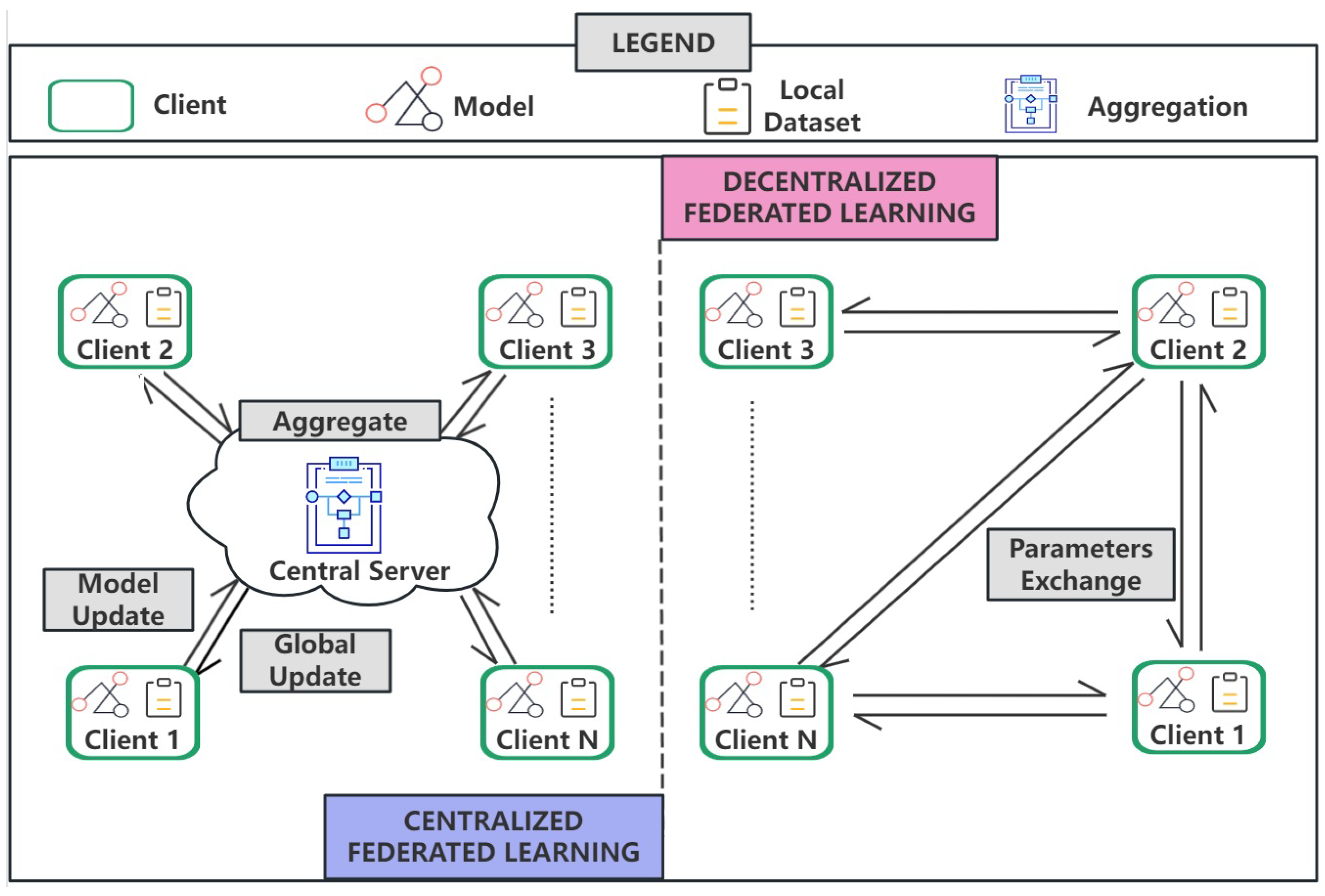
The FL, as shown in Figure 1, has two architectures. In centralized FL, each client trains the model utilizing its local data. Subsequently, each client uploads the updated model to the central server. Upon receiving model updates from clients, the central server combines the model parameters to create a unified global model update. The central server then dispatches the unified global model update to each individual client. This process iterates until the model completes the designated training epochs. This server globally coordinates the training process of the model, ensuring that each client contributes to the improvement of the overall model. However, this architecture has certain limitations; for example, in large-scale FL systems, the central server may become a performance bottleneck, and in some cases, centralized data aggregation may raise concerns related to privacy and security.

In the DFL framework, each client initiates local training using its own dataset, subsequently updating its local model. Clients then engage in direct communication, exchanging model parameters or gradient information. Upon receiving data from other clients, each client aggregates this information with its local model, resulting in an updated local model. This iterative process allows DFL to execute federated learning tasks across distributed devices, with each client contributing insights from its raw data without the need to transmit the data to a central server, thus maintaining data privacy. This method of direct communication mitigates communication latency, enhances real-time system responsiveness, and reduces reliance on a central server, thereby increasing system flexibility and decentralization. Consequently, DFL is well suited for machine learning scenarios that prioritize decentralization, collaboration, and privacy protection.

2.2. Problem Formulation

Suppose a directed graph $\mathcal{G}=\{C,\mathcal{E},A_t\}$ with the set of n clients $C:=\{1,\dots ,n\}$, the communication channels $\mathcal{E}\subseteq C\times C$, and the adjacency matrix $A_t\in {\mathbb{R}}^{n\times n}$. For each pair $\left(i,j\right)\in \mathcal{E}$, there exists an information transmission channel from client i to client j at time t. When i is regarded as an in-neighbor of j, j is regarded as out-neighbor of i in contrast. Regarding ${\mathcal{N}}_{i,in}^t=\{j\subseteq C|(j,i)\in \mathcal{E}\}\cup \left\{i\right\}$ as the in-neighbors set of i at time t, the adjacency matrix obeys when ${\left[A_t\right]}_{ij}>0$ if $j\in {\mathcal{N}}_{i,in}^t$, and there is a positive scalar $\zeta$ such that ${\left[A_t\right]}_{ij}>\zeta ,t\in \left\{1,\dots ,T\right\}$. Further, $A_t$ is doubly-stochastic which satisfies ${\sum }_{j=1}^n{\left[A_t\right]}_{ij}={\sum }_{i=1}^n{\left[A_t\right]}_{ij}=1$ for all $\left(i,j\right)\in C$, for any $t\in \left\{1,\dots ,T\right\}$.

Assumption 1.

For any $Q\in {\mathbb{Z}}_{+}$, the combined graph ${\bigcup }_{i=kQ+1}^{\left(k+1\right)Q}{\mathcal{G}}_i$ exhibits strong connectivity for all integers $k\ge 0$.

Remark 1.

For the definition of the spectral gap parameter $\lambda$, let $W_t=A_t^{\top }{A}_t$ be the mixing matrix at time t. We define $\lambda \in [0,1)$ as the uniform upper bound on the second largest singular value of $\mathbb{E}\left[W_t\right]$, i.e., $\lambda \ge {\sigma }_2\left(\mathbb{E}\left[W_t\right]\right)$, for all t, where ${\sigma }_2(·)$ denotes the second largest singular value. The term $(1-\lambda )$ represents the spectral gap of the expected communication network, which quantifies the connectivity and consensus speed of the graph. A smaller $\lambda$ (larger spectral gap) indicates faster information diffusion across the network.

At each iteration $t\in \left\{1,\dots ,T\right\}$, consider a federated learning scenario where each client i trains a model locally, and the client’s dataset $d_i$ is non-IID. The probability density function for each client is represented as $f_i$, and distinct data distribution can be represented as follows: $f_1\left(d_1\right)\ne f_2\left(d_2\right)\ne \dots f_n\left(d_n\right)$. Specifically, each client performs an action $z_i^t\in Z,Z\subset {\mathbb{R}}^d$, where Z is a convex and compact feasible set. Additionally, based on local data, each client computes a time-varying local loss function $l_i^t:{\mathbb{R}}^d\to \mathbb{R}$. Subsequently, each client collaboratively updates the model with others through information exchange. The primary objective is to minimize the cumulative local cost functions of all clients, i.e.,

$$\underset{z\in Z}{\min }\sum _{t=1}^T\sum _{i=1}^n{l}_i^t\left(z;d_i\right),$$

(1)

where function l is differentiable and whose gradient is symbolized as $\nabla l\left(·\right)$.

The function is called K-smooth over a given convex set Z when it satisfies

$$l_i^t\left(a\right)-l_i^t\left(b\right)\le 〈\nabla l_i^t\left(b\right),a-b〉+{\displaystyle \frac{K}{2}}{∥a-b∥}^2,\forall a,b\in Z,$$

where K is a positive constant. The function is convex on a convex set Z when it satisfies

$$l_i^t\left(a\right)-l_i^t\left(b\right)\ge 〈\nabla l_i^t\left(b\right),a-b〉,\forall a,b\in Z.$$

To evaluate the algorithm’s performance, we introduce regret. Regret is the difference between the total cost over all iterations and the cost of the optimal fixed choice when all functions are known beforehand. For each client j, its individual dynamic regret is defined as below

$$R_j^T=\sum _{t=1}^T\sum _{i=1}^n{l}_i^t\left(z_j^t\right)-\sum _{t=1}^T\sum _{i=1}^n{l}_i^t\left(z_{*}^t\right),$$

(2)

where $z_{*}^t\in arg{min}_{z\in Z}{\sum }_{t=1}^T{\sum }_{i=1}^n{l}_i^t\left(z\right)$. The objective is to make sure the algorithm obtains the dynamic regret satisfying the sublinear condition, i.e., $li{m}_{T\to \infty }\left(R_j^T/T\right)=0,\forall j\in C$.

It is widely recognized that dynamic regret cannot attain sublinear convergence unless the variation budget exhibits sublinear dependence on T. Keep in consideration that the variations in the function, denoted as $H_T$, and the gradient variation, denoted as $D_T$, associated with the bound of $R_j^T$, are defined as follows:

$$H_T=\sum _{t=1}^T\underset{i\in C}{max}\underset{z\in Z}{max}\left|l_i^{t+1}\left(z\right)-l_i^t\left(z\right)\right|,$$

(3)

$$D_T=\sum _{t=1}^T\underset{i\in C}{max}\underset{z\in Z}{max}∥\nabla l_i^{t+1}\left(z\right)-\nabla l_i^t\left(z\right)∥.$$

(4)

The following assumptions are typically introduced as the foundation for analyzing and demonstrating the performance of algorithms.

Assumption 2.

Local convex cost function $l_i^t$ is $L_i$-Lipschitz for all $i\in C$, i.e., $\forall z_1,z_2\in C$, $\left|l_i^t\left(z_1\right)-l_i^t\left(z_2\right)\right|\le L_i∥z_1-z_2∥$, in which ${\sum }_{i=1}^n{L}_i=L$.

Assumption 3.

Subgradient $\nabla l_i^t\left(z\right)$ of $l_i^t\left(z\right)$ at z is G-Lipschitz, i.e., for $\forall z_1,z_2\in Z$, $∥\nabla l_i^t\left(z_1\right)-\nabla l_i^t\left(z_2\right)∥\le G∥z_1-z_2∥$.

Assumption 4.

The constraint set Z holds a finite diameter M, namely, for $\forall z_1,z_2\in Z$, $su{p}_{z_1,z_2\in Z}∥z_1-z_2∥\le M$.

In distributed optimization, Assumptions 2 and 3 are standard setting such as in [20]. According to Lemma 2.6 in [38], Assumption 2 implies $∥\nabla l_i^t\left(z\right)∥\le L_i$. Although deep neural networks typically exhibit non-convex loss function surfaces, Assumptions 2–4 provide a controlled framework to rigorously analyze the interaction between differential privacy noise and optimization dynamics; establish sublinear regret bounds quantifying performance in non-stationary environments; and isolate the effects of gradient tracking in decentralized settings. Empirical validation in Section 4 will examine how insights gained from convexity analysis translate to non-convex practical scenarios.

Remark 2.

The doubly-stochastic condition on $A_t$ assumes a bounded-delay synchronization model within each communication round, which is a common technical assumption in decentralized consensus analysis. In practice, the weights can be generated locally (e.g., via the Metropolis rule) based on the known neighborhood structure, requiring only that all neighbors eventually exchange information within a round. This model does not require strict global clock alignment but implies that nodes are loosely synchronized. If a neighbor is temporarily unavailable, the node uses the most recent information received from that neighbor.

2.3. Differential Privacy

In this section, the definition and related concepts of differential privacy are introduced. The formal definition of $ϵ$-differential privacy for a stochastic mechanism ${\mathcal{M}}_{\mathcal{C}}$ with the parameter $ϵ$ is provided. To achieve differential privacy, we then introduce the concept of sensitivity.

Definition 1.

For $ϵ>0,\delta >0$, a random mechanism ${\mathcal{M}}_{\mathcal{C}}$ is ϵ-differentially private if for all δ-adjacent function sets only one record in both data sets is disparate and if any S or $S^{\prime }$ for all events O in the out space of ${\mathcal{M}}_{\mathcal{C}}$, ${\mathcal{M}}_{\mathcal{C}}$ satisfies

$$P_r\left({\mathcal{M}}_{\mathcal{C}}\left(S\right)\in O\right)\le e^{ϵ}·P_r\left({\mathcal{M}}_{\mathcal{C}}\left(S^{\prime }\right)\in O\right).$$

(5)

The concept of $ϵ$-differential privacy highlights that a minor alteration in the private dataset will not substantially impact the algorithm’s output. Hence, the algorithm produces a closer output set when processing adjacent data sets S and $S^{\prime }$. $ϵ>0$ signifies the degree of privacy protection offered by mechanism ${\mathcal{M}}_{\mathcal{C}}$. A smaller $ϵ$ indicates stronger privacy protection.

We adopt the local differential privacy (LDP) model, where each client perturbs its shared information locally before transmission. This contrasts with centralized DP that requires a trusted aggregator. This paper adopts the local differential privacy model. Each client independently adds Laplace noise before sending information to its neighbors.

Definition 2.

The ${\mathsf{\ell }}_1$-sensitivity of Algorithm 1 at iteration t is defined as follows:

$${\mathrm{\Delta }}_t=\underset{D\sim D^{\prime }}{sup}{∥{\mathcal{M}}_{\mathcal{C}}\left(D_t\right)-{\mathcal{M}}_{\mathcal{C}}\left(D_t^{\prime }\right)∥}_1,$$

(6)

where $D_i\sim D_i^{\prime }$ denotes two adjacent local datasets that differ in a single entry.

Sensitivity indicates the extent to which altering a solitary individual’s data can influence the algorithm. It plays a crucial role in deciding the amount of perturbation needed to ensure a specific level of privacy preservation. Consequently, we can manage the intensity of stochastic noise by limiting sensitivity, ensuring the enforcement of differential privacy. Consequently, we can manage the intensity of stochastic noise by limiting sensitivity, ensuring the enforcement of differential privacy.

3. Algorithm Design

3.1. Algorithm

This section proposes the DPDOPFO algorithm. Its core design revolves around three objectives: avoiding the projection overhead in high-dimensional constrained settings, protecting local data privacy during communication, and mitigating optimization bias caused by non-IID client data through a gradient tracking mechanism. In each iteration, each client executes the following collaborative process in parallel: First, noise-injected weighted average consensus (8) is executed based on time-varying communication topologies. Laplace noise (${\gamma }_j^t$) is added during neighborhood model aggregation to provide preliminary privacy protection, yielding a local estimated model. Subsequently, the gradient tracking phases (9) and (10) dynamically integrate local and neighborhood gradient information, supplemented by gradient information noise (${\eta }_j^t$), to more accurately approximate the global gradient direction while ensuring privacy. Subsequently, the Frank–Wolfe algorithm (11) solves the linear subproblem over the feasible set to directly obtain the descent direction, completely avoiding the computational burden of traditional projection operations. Finally, the local model is updated (12) along this direction with a step size $\alpha$, ensuring that the iterate always remains within the feasible domain. The entire algorithm operates within a fully decentralized architecture, achieving strict $ϵ$-differential privacy through noise injection, and enables efficient and stable collaborative learning in environments with complex constraints and data heterogeneity via gradient tracking and projection-free updates.

In the context of federated learning, this algorithm leverages communication and model updates among decentralized clients to achieve differentially private projection-free optimization over multiple iterations. The average consensus step facilitates information exchange among clients, while the Frank–Wolfe steps ensure that model updates remain within the feasible set, all while maintaining differential privacy. This algorithm exemplifies the collaborative and privacy-preserving nature of federated learning, effectively balancing the need for distributed computation with stringent privacy requirements. In terms of complexity, each iteration requires solving a linear optimization subproblem, which for common constraint sets such as the ${\mathsf{\ell }}_1$-ball or nuclear-norm ball incurs a cost of $O(dlogd)$ or $O\left(d^3\right)$ (SVD), respectively, while traditional projected gradient descent (e.g., pSGD) typically needs $O\left(d^2\right)$ projection operations. The per-round communication cost is $O\left(\right|\mathcal{E}|·d)$, where $\left|\mathcal{E}\right|$ is the number of edges in the communication graph, and the overhead of adding Laplace noise is only $O\left(d\right)$ per node, which does not dominate the overall complexity.

Remark 3.

As shown in Equations (7) and (8), each client i transmits both the local model $z_i^t$ and the gradient tracking variable $s_i^t$ to its neighbors in every round, resulting in a per-round communication payload of $2d$ floats per link. This is double the cost of algorithms that only share gradients (e.g., DGD) or models (e.g., decentralized FedAvg). The purpose of sharing $s_i^t$ is to enable gradient tracking, which is critical for achieving fast consensus on the global gradient direction under time-varying networks and non-IID data distributions. While this increases the per-round communication cost, it significantly accelerates convergence and reduces the total number of communication rounds required to reach a target accuracy.

3.2. Complexity Analysis

To justify the projection-free advantage of DPDOPFO, we analyze the computational complexity per iteration and compare it with projection-based methods. The computational cost of DPDOPFO consists of three main components: (1) the consensus step (Equation (7)), (2) gradient tracking (Equations (8) and (9)), and (3) the Frank–Wolfe linear oracle (Equation 10). While the consensus and gradient tracking operations have standard O(d) complexity for d-dimensional vectors, the Frank–Wolfe step requires special attention.

The complexity of this operation depends critically on the structure of the constraint set Z.

Table 1. Computational complexity comparison between Frank–Wolfe linear oracle and projection operations for different constraint sets.

Constraint Set Z	Frank–Wolfe Linear Oracle	Projection Operation
Simplex	$O(dlogd)$	$O(dlogd)$
${\mathsf{\ell }}_1$-ball	$O(dlogd)$	$O(dlogd)$
${\mathsf{\ell }}_2$-ball	$O\left(d\right)$	$O\left(d\right)$
Nuclear norm ball	$O(k·mn)$	$O(mn·min(m,n\left)\right)$
Trace norm ball	$O(r·d^2)$	$O\left(d^3\right)$
Polytope	$O\left(md\right)$ n	$O\left(m{d}^2\right)$

provides a detailed comparison of computational complexities for different constraint sets commonly encountered in federated learning applications. The constraint set Z includes simplex $({\mathrm{\Delta }}_d=x\in {\mathbb{R}}^d:x\ge 0,{\sum }_{i=1}^d{x}_i=1)$; ${\mathsf{\ell }}_1$-ball $\left(x\in {\mathbb{R}}^d:{\left|x\right|}_1\le r\right)$; ${\mathsf{\ell }}_2$-ball $\left(x\in {\mathbb{R}}^d:\left|x\right|2\le r\right)$; nuclear norm ball ($X\in {\mathbb{R}}^{m\times n}:\left|X\right|*\le r,$ using rank-k approximation); trace norm ball with rank constraint; and polytope $\left(x:Ax\le b\right)$ with m constraints.

For many structured constraint sets commonly encountered in machine learning—particularly those promoting sparsity or low rank—the Frank–Wolfe linear oracle demonstrates higher computational efficiency compared to projection methods. Specifically: (1) for low-rank matrix constraints (e.g., kernel norm ball constraints), the Frank–Wolfe algorithm requires only rank-k singular value decomposition (SVD), with complexity $O(k·mn)$, whereas the full projection method requires $O(mn·min(m,n\left)\right)$. When $k\ll min(m,n)$, an acceleration factor of $O(min(m,n)/k)$ is achieved; (2) for sparse vector constraints (e.g., ${\mathsf{\ell }}_1$ ball constraints), both methods exhibit theoretical complexity of $O(dlogd)$. However, the Frank–Wolfe algorithm naturally produces sparse iteration results (with at most t nonzero elements after t iterations), thereby reducing memory and computational overhead in subsequent steps; (3) for decomposable constraints (Cartesian products of simple sets), the Frank–Wolfe algorithm employs coordinate decomposition, supporting parallel computation and reducing complexity from $O\left(d^3\right)$ in the projection method to $O\left({\sum }_j{d}_j^3\right)$. In practice, for bounded convex sets considered under Assumption 4, we implement an efficient structure-adaptive approach for the linear oracle. The Frank–Wolfe algorithm maintains high efficiency even in high-dimensional neural network experiments—thanks to its simple oracle operations (e.g., extremum coordinate selection), inherent sparse/low-rank update properties, and reduced need for hyperparameter tuning related to projection.

Moreover, the per-iteration communication cost of DPDOPFO is $O\left(d\right)$, identical to projection-based distributed methods, while the computational advantage $T_{\mathrm{DPDOPFO}}/T_{\mathrm{Proj}}$ often falls below one for structured constraints, justifying the projection-free approach. For unconstrained cases, both methods exhibit similar costs, yet DPDOPFO retains advantages in numerical stability and avoidance of projection-related issues.

We further analyze the communication cost of DPDOPFO. Per iteration, each client transmits both its model parameter $z_i^t$ and its gradient tracking variable $s_i^t$ to neighbors, resulting in a per-round communication volume of $O\left(2d\right)$ per link, compared to $O\left(d\right)$ for DGD that transmits only gradients. However, gradient tracking crucially reduces the variance of gradient estimates in decentralized settings with non-IID data and time-varying objectives, which in turn significantly decreases the number of communication rounds T required to reach a target accuracy. The total communication cost over T rounds is $O(2d·T_{\mathrm{DPDOPFO}})$. Our theoretical bound in Lemma 2(c) and the regret analysis in Theorem 2 show that the term involving $\sum \parallel d_i^t\parallel$, while growing with T, is essential for controlling the optimization error caused by data heterogeneity; without it, the required T would be substantially larger. In practice, for non-IID data, the reduction in T often outweighs the per-round cost doubling. Compared to variance-reduced methods like SAGA, DPDOPFO operates in a fully decentralized online setting without requiring storage of past gradients, making it more suitable for resource-constrained edge devices.

3.3. Convergence Results

In this part, we demonstrate that DPDOPFO ensures $(ϵ,\delta )$-differential privacy and analyze the dynamic regret upper bound defined in (2). Before presenting the formal lemmas and theorems, we outline the proof strategy to provide intuition. The analysis must address three challenges in the time-varying private network: consensus error under privacy noise, gradient tracking error in non-IID settings, and the propagation of noise through iterations. Our strategy first bounds the consensus and gradient tracking errors and then integrates these bounds with the properties of the Frank–Wolfe update to establish the final regret guarantee. For this purpose, we first introduce several lemmas, followed by the presentation of the main results.

Then we provide the condition of the stochastic noise ${\pi }_i^t$ as follows.

Assumption 5.

The stochastic noises ${\pi }_i^t,i\in C,t\in \left\{1,\cdots ,T\right\}$ together comprise a stochastic variable which is independent and satisfies $\mathbb{E}\left[{\pi }_i^t\mid {\mathcal{F}}_{t-1}\right]=0$. Also, presume that $\mathbb{E}\left[∥{\pi }_i^t∥\right]\le {\tau }_i$.

Bounding the sensitivity helps determine a suitable quantity of stochastic noises to achieve $ϵ$-differential privacy. Thus, we initially constrain the sensitivity of DPDOPFO as follows.

Lemma 1.

Presuming that Assumption 4 holds, the sensitivity of Algorithm 1 has an upper limit

$$\begin{array}{c}\hfill {\mathrm{\Delta }}_t\le \alpha \sqrt{d}M.\end{array}$$

(7)

Algorithm 1: Differentially Private Decentralized Online Projection-Free Optimization (DPDOPFO)

Input: any client $i\in C$: Epoch T, Initialized Model $z_1^i\in Z$, Initialized Gradient $s_i^1=\nabla l_i^t\left({\widehat{z}}_i^1\right)$. for $t=1$ to T do    Average Consensus: $${\widehat{z}}_i^t=\sum _{j\in {\mathcal{N}}_i}{\left[A_t\right]}_{ij}\left(z_j^t+{\gamma }_j^t\right),$$ (8)     where ${\mathcal{N}}_{i,in}^t$ is client i’s in-neighbors set.    Gradient Tracking: $$\begin{array}{cc}\hfill & p_i^t=\sum _{j\in {\mathcal{N}}_i}{\left[A_t\right]}_{ij}\left(s_j^t+{\eta }_j^t\right),\hfill \end{array}$$ (9) $$\begin{array}{cc}\hfill & s_i^{t+1}=p_i^t+\nabla l_i^{t+1}\left({\widehat{z}}_i^{t+1}\right)-\nabla l_i^t\left({\widehat{z}}_i^t\right).\hfill \end{array}$$ (10)    Frank–Wolfe steps: $$\begin{array}{cc}\hfill & {\theta }_i^t=\underset{\psi \in Z}{argmin}〈s_i^t,\psi 〉,\hfill \end{array}$$ (11) $$\begin{array}{c}\hfill z_i^{t+1}={\widehat{z}}_i^t+\alpha \left({\theta }_i^t-{\widehat{z}}_i^t\right),\end{array}$$ (12)    where step size satisfies $0<\alpha \le 1.$ end return $z_{t+1}^i$ for all client $i\in C$.

Next, we present the theorem and its proof guaranteeing $ϵ$-differential privacy for DPDOPFO.

Theorem 1.

Under Assumptions 4 and 5, and given that the noise ${\gamma }_i^t$ is drawn i.i.d. from $\mathit{Lap}{(0,\sigma )}^d$ with scale $\sigma ={\mathrm{\Delta }}_t/{ϵ}_0$, the overall execution of Algorithm 1 over T rounds satisfies $(ϵ,\delta )$-differential privacy. The total privacy budget $ϵ$ is given by the advanced composition theorem: $ϵ={ϵ}_0\sqrt{2Tln(1/\delta )}+T{ϵ}_0(e^{{ϵ}_0}-1)$ for any $\delta >0$, where ${ϵ}_0$ is the single-round privacy parameter.

Proof of Theorem 1.

Recall the definition in (6); it has

$${∥z_i^{t+1}-{\left(z_i^{t+1}\right)}^{\prime }∥}_1\le {\mathrm{\Delta }}_t.$$

Then, in accordance with the Laplace distribution, it is sufficient that

$$\begin{array}{cc}\hfill \mathrm{\prod }_{i=1}^n\mathrm{\prod }_{k=1}^d{\displaystyle \frac{Pr\left[x_{i,k}^t-z_{i,k}^t\right]}{Pr\left[x_{i,k}^t-{\left(z_{i,k}^t\right)}^{\prime }\right]}}& \le \mathrm{\prod }_{i=1}^n\mathrm{\prod }_{k=1}^{d}exp\left({\displaystyle \frac{\left|x_{i,k}^t-{\left(z_{i,k}^t\right)}^{\prime }-x_{i,k}^t+z_{i,k}^t\right|}{{\sigma }_t}}\right)\hfill \\ \hfill & \le exp\left({\displaystyle \frac{∥z_{i,k}^t-{\left(z_{i,k}^t\right)}^{\prime }∥}{{\sigma }_t}}\right)\hfill \\ \hfill & \le exp\left({\displaystyle \frac{{\mathrm{\Delta }}_t}{{\sigma }_t}}\right).\hfill \end{array}$$

(13)

Further, it has

$$P_r\left({\mathcal{M}}_{\mathcal{C}}\left(S\right)\in O\right)=\mathrm{\prod }_{t=1}^{T}Pr\left[{\mathcal{M}}_{\mathcal{C}}\left(S_t\right)\in O\right].$$

Integrate both sides of (13) with the last equation; then, the following is obtained:

$$\mathrm{\prod }_{t=1}^{T}Pr\left[{\mathcal{M}}_{\mathcal{C}}\left(S_t\right)\in O\right]\le \mathrm{\prod }_{t=1}^{T}exp\left({\displaystyle \frac{{\mathrm{\Delta }}_t}{{\sigma }_t}}\right)·Pr\left[{\mathcal{M}}_{\mathcal{C}}\left({S_t}^{\prime }\right)\in O\right],$$

which in accordance with ${\displaystyle \frac{{\mathrm{\Delta }}_t}{{\sigma }_t}}=\epsilon$ yields that

$$Pr\left[{\mathcal{M}}_{\mathcal{C}}\left(S\right)\in O\right]\le exp\left(\epsilon \right)·Pr\left[{\mathcal{M}}_{\mathcal{C}}\left(S^{\prime }\right)\in O\right]$$

and by the definition in (5), the proof is completed.    □

To simplify the proof and analysis, we introduce the concept of the max function variation $V_f^t$ at time t, the max gradient variation $V_g^t$ at time t and difference of gradient $d_i^t$ of agent i as below:

$$\begin{array}{cc}\hfill V_f^t& =\underset{i\in C}{max}\underset{z\in Z}{max}\left|l_i^{t+1}\left(z\right)-l_i^t\left(z\right)\right|,\hfill \end{array}$$

(14)

$$\begin{array}{cc}\hfill V_g^t& =\underset{i\in C}{max}\underset{z\in Z}{max}∥\nabla l_i^{t+1}\left(z\right)-\nabla l_i^t\left(z\right)∥,\hfill \end{array}$$

(15)

$$\begin{array}{cc}\hfill d_i^t& =\nabla l_i^t\left({\widehat{z}}_i^t\right)-\nabla l_i^{t-1}\left({\widehat{z}}_i^{t-1}\right).\hfill \end{array}$$

(16)

The convergence analysis of Algorithm 1 relies on the essential lemmas presented below.

Lemma 2.

The decision sequence $\left\{z_i^t\right\}$ is yielded by Algorithm 1. Under Assumptions 2–4, for any $T\ge 2$, it has

(a) 

${\sum }_{i=1}^n{s}_i^{t+1}={\sum }_{i=1}^n\nabla l_i^{t+1}\left({\widehat{z}}_i^{t+1}\right)+{\sum }_{i=1}^n{\sum }_{l=1}^t{\eta }_i^l$,

(b) 

${\overline{z}}^{t+1}={\overline{z}}^t+{\overline{\gamma }}^t+{\displaystyle \frac{\alpha }{n}}{\sum }_{i=1}^n\left({\theta }_i^t-{\widehat{z}}_i^t\right)$,

(c) 

${\sum }_{t=2}^T{\sum }_{i=1}^n∥d_i^t∥\le 2G{\sum }_{t=2}^T{\sum }_{i=1}^n∥{\widehat{z}}_i^{t-1}-{\overline{z}}^{t-1}∥+n{D}_T+\alpha TnMG+G{\sum }_{t=2}^T{\sum }_{i=1}^n∥{\gamma }_i^t∥$.

Lemma 3.

By Assumption 4 and the property of the adjacency matrix $A_t$, consider the decision sequence $\left\{z_i^t\right\}$ produced by Algorithm 1; then, for $T\ge 2$, the following is obtained:

$$\begin{array}{cc}\hfill \mathbb{E}\left[\sum _{t=1}^T\sum _{i=1}^n∥{\widehat{z}}_i^t-{\overline{z}}^t∥\right]\le & {\displaystyle \frac{n\Gamma }{1-\lambda }}\sum _{j=1}^n∥z_j^1∥+{\displaystyle \frac{\alpha T{n}^{2}M\Gamma }{1-\lambda }}+\left({\displaystyle \frac{n\Gamma }{1-\lambda }}+n\right){\displaystyle \frac{\sqrt{2}ndM\alpha T}{\epsilon }}.\hfill \end{array}$$

Lemma 4.

Let the sequence $\left\{p_i^t,\nabla l_i^t\left({\widehat{z}}_i^t\right)\right\}$ be generated by Algorithm 1; then, by the property of adjacency matrix and Assumption 2, for any $T\ge 2$, it holds that

$$\begin{array}{cc}\hfill \sum _{t=1}^T\sum _{i=1}^n∥p_i^t-{\displaystyle \frac{1}{n}}\sum _{j=1}^n\nabla l_j^t\left({\widehat{z}}_j^t\right)∥\le & {\displaystyle \frac{n\Gamma }{1-\lambda }}\sum _{j=1}^n∥\nabla l_j^1\left({\widehat{z}}_j^1\right)∥+{\displaystyle \frac{n\Gamma }{1-\lambda }}\sum _{t=2}^T\sum _{i=1}^n∥d_i^t∥\hfill \\ \hfill & +{\displaystyle \frac{n\Gamma }{1-\lambda }}\sum _{t=2}^T\sum _{i=1}^n∥{\eta }_i^t∥.\hfill \end{array}$$

(17)

Lemma 5.

Algorithm 1 generates the decision sequence denoted as $\left\{z_i^t\right\}$. Then, under Assumptions 2–4, for any $T\ge 2$, the following is achieved:

$$\begin{array}{cc}\hfill \sum _{t=1}^T{l}_i^t\left({\overline{z}}^t\right)-\sum _{t=1}^T{l}_i^t\left(z_{*}^t\right)\le & {\displaystyle \frac{2H_T}{\alpha }}+{\displaystyle \frac{L_{i}M}{\alpha }}+M{D}_T+2M\sum _{t=1}^{T-1}\sum _{i=1}^n∥{\displaystyle \frac{1}{n}}\sum _{j=1}^n\nabla l_j^t\left({\widehat{z}}_j^t\right)-p_i^t∥\hfill \\ \hfill & +{\displaystyle \frac{2MG}{n}}\sum _{t=1}^{T-1}\sum _{j=1}^n∥{\widehat{z}}_j^t-{\overline{z}}^t∥+{\displaystyle \frac{K{M}^2\alpha T}{2}}+{\displaystyle \frac{L_i}{\alpha }}∥{\overline{\gamma }}^t∥.\hfill \end{array}$$

(18)

In this part, a detailed analysis of the upper bound for the dynamic regret, as defined in Formula (2), is given for Algorithm 1.

Theorem 2.

Presume Assumptions 2–5 hold. Consider Algorithm 1 generates the decision sequence $\left\{z_i^t\right\}$. Then, for $T\ge 2$ and $j\in C$, the dynamic regret is bounded as below

$$\begin{array}{c}\hfill \mathbb{E}\left[R_j^T\right]\le A_1+A_2\alpha T+{\displaystyle \frac{2n}{\alpha }}{H}_T+{\displaystyle \frac{A_3}{\alpha }}+A_4{D}_T,\end{array}$$

(19)

where

$$\begin{array}{cc}\hfill A_1& =L\sum _{i=1}^n∥{\widehat{z}}_i^1-{\overline{z}}^1∥+{\displaystyle \frac{2M{n}^2\Gamma }{1-\lambda }}\sum _{i=1}^n∥\nabla l_i^1\left({\widehat{z}}_i^1\right)∥+{\displaystyle \frac{\sqrt{2}dML}{\epsilon }}\hfill \\ \hfill & +{\displaystyle \frac{n\Gamma }{1-\lambda }}\left(L+2MG+{\displaystyle \frac{4MG{n}^2\Gamma }{1-\lambda }}\right)\sum _{i=1}^n∥z_i^1∥,\hfill \\ \hfill A_2& =2nLM+{\displaystyle \frac{n^{2}M\Gamma }{1-\lambda }}\left(L+2MG+2nMG+{\displaystyle \frac{4MG{n}^2\Gamma }{1-\lambda }}\right)+{\displaystyle \frac{K{M}^{2}n}{2}}\hfill \\ \hfill & +\left({\displaystyle \frac{n\Gamma }{1-\lambda }}+n\right){\displaystyle \frac{\sqrt{2}ndM}{\epsilon }}\left(L+{\displaystyle \frac{4MG{n}^2\Gamma }{1-\lambda }}\right)\hfill \\ \hfill & +{\displaystyle \frac{\sqrt{2}dM}{\epsilon }}\left({\displaystyle \frac{2M{n}^3\Gamma }{1-\lambda }}+{\displaystyle \frac{2MG{n}^3\Gamma }{1-\lambda }}+L\right),\hfill \\ \hfill A_3& =LM,A_4=nM+{\displaystyle \frac{2M{n}^3\Gamma }{1-\lambda }}.\hfill \end{array}$$

Proof of Theorem 2.

By Assumption 2,

$$\begin{array}{cc}\hfill \mathbb{E}\left[R_j^T\right]=& \mathbb{E}\left[\sum _{t=1}^T\sum _{i=1}^n\left(l_i^t\left(z_j^t\right)-l_i^t\left(z_{*}^t\right)\right)\right]\hfill \\ \hfill =& \mathbb{E}\left[\sum _{t=1}^T\sum _{i=1}^n\left(l_i^t\left(z_j^t\right)-l_i^t\left({\overline{z}}^t\right)+l_i^t\left({\overline{z}}^t\right)-l_i^t\left(z_{*}^t\right)\right)\right]\hfill \\ \hfill \le & \mathbb{E}\left[\sum _{t=1}^T\sum _{i=1}^n\left(L_i∥z_j^t-{\overline{z}}^t∥+l_i^t\left({\overline{z}}^t\right)-l_i^t\left(z_{*}^t\right)\right)\right].\hfill \end{array}$$

(20)

Based on Lemma 2(b) and the Algorithm 1, for any $t\ge 2$, the following is obtained:

$$\begin{array}{cc}\hfill ∥z_i^t-{\overline{z}}^t∥=& ∥{\widehat{z}}_i^{t-1}+\alpha ({\theta }_i^{t-1}-{\widehat{z}}_i^{t-1})-{\overline{z}}^{t-1}-{\overline{\gamma }}^{t-1}-{\displaystyle \frac{\alpha }{n}}\sum _{i=1}^n\left({\theta }_i^t-{\widehat{z}}_i^t\right)∥\hfill \\ \hfill =& ∥{\widehat{z}}_i^{t-1}-{\overline{z}}^{t-1}+\alpha ({\theta }_i^{t-1}-{\widehat{z}}_i^{t-1})-\alpha ({\overline{\theta }}^{t-1}-{\overline{z}}^{t-1})-\alpha {\overline{\gamma }}^{t-1}∥\hfill \\ \hfill \le & ∥{\widehat{z}}_i^{t-1}-{\overline{z}}^{t-1}∥+2\alpha M+∥{\overline{\gamma }}^{t-1}∥.\hfill \end{array}$$

(21)

Recalling the notion of individual regret, the following is obtained:

$$\begin{array}{cc}\hfill \mathbb{E}\left[R_j^T\right]\le & \mathbb{E}\left[\sum _{t=2}^{T-1}\sum _{i=1}^n{L}_i\left(∥{\widehat{z}}_i^t-{\overline{z}}^t∥+∥{\overline{\gamma }}^t∥\right)\right]+\mathbb{E}\left[\sum _{i=1}^n{L}_i(∥{\widehat{z}}_i^1-{\overline{z}}^1∥+∥{\overline{\gamma }}^1∥)\right]\hfill \\ \hfill & +2nLM\alpha T+\mathbb{E}\left[\sum _{t=1}^T\sum _{i=1}^n\left(l_i^t\left({\overline{z}}^t\right)-l_i^t\left(z_{*}^t\right)\right)\right]\hfill \\ \hfill \le & L\sum _{i=1}^n∥{\widehat{z}}_i^1-{\overline{z}}^1∥+L\sum _{t=1}^{T-1}\sum _{i=1}^n∥{\widehat{z}}_i^t-{\overline{z}}^t∥+L{\displaystyle \frac{\sqrt{2}dM\alpha T}{\epsilon }}+2nLM\alpha T\hfill \\ \hfill & +\mathbb{E}\left[\sum _{t=1}^T\sum _{i=1}^n\left(l_i^t\left({\overline{z}}^t\right)-l_i^t\left(z_{*}^t\right)\right)\right].\hfill \end{array}$$

(22)

This inequality, together with Lemma 2(c) and Lemmas 3–5, readily achieves the result in Theorem 2. The proof is complete.    □

The main outcomes related to dynamic regret are presented in Theorem 2. It is worth noting that the regret bound of Algorithm 1 is contingent on the choice of $\alpha$. Therefore, we can derive the following corollary by selecting appropriate step sizes.

Corollary 1.

Presume that the condition in Theorem 2 holds. After that, if $H_T=\mathcal{O}\left(T\right),D_T=\mathcal{O}\left(T\right)$ holds, taking $\alpha =\beta \sqrt{{\displaystyle \frac{H_T+1}{T}}}$, the following is obtained:

$$\begin{array}{c}\hfill R_j^T\le \mathcal{O}\left(\sqrt{T\left(H_T+1\right)}+D_T\right),\end{array}$$

(23)

where β is a positive adjustment constant to guarantee $\alpha \le 1$.

Proof of Corollary 1.

According to Theorem 2, $R_j^T\le \mathcal{O}\left(\alpha T+D_T+{\displaystyle \frac{1}{\alpha }}\left(1+H_T\right)\right)$. After that, (23) is readily achieved by taking $\alpha T={\displaystyle \frac{1}{\alpha }}\left(1+H_T\right)$. The proof is complete.    □

Remark 4.

Corollary 1 aligns with the centralized result in [39], offering a tighter bound than the upper limit of $\mathcal{O}\left(\sqrt{T}\left(1+H_T+\sqrt{D_T}\right)\right)$ with the same linear oracle complexity. Moreover, our approach extends the range of $H_T$ from $\mathcal{O}\left(\sqrt{T}\right)$ to $\mathcal{O}\left(T\right)$ in [39], achieving a sublinear regret bound, effectively expanding the applicability to optimization problems. To further interpret the result, the bound $\mathcal{O}(\sqrt{T(H_T+1)}+D_T)$ explicitly quantifies the cost of environmental non-stationarity ($H_T$ and $D_T$) and the overhead of decentralization and privacy (absorbed in the constants $A_1$–$A_4$). The term $\sqrt{T(H_T+1)}$ is fundamental to online learning in drifting environments, while the additive $D_T$ term captures the impact of gradient variability. Compared to prior decentralized Frank–Wolfe analyses (e.g., [22,24]), our bound explicitly incorporates the effects of time-varying graphs and local differential privacy.

4. Simulation Results

In this section, we leverage Algorithm 1 as a foundational framework for conducting decentralized federated learning experiments. The efficacy of Algorithm 1 is demonstrated through experiments conducted on FashionMNIST and MNIST datasets, simulating scenarios involving non-IID data distributions. By conducting these simulations, our goal is to validate the efficacy of the suggested algorithm.

4.1. Experimental Settings

All experiments are conducted under a unified configuration. Using the MNIST and Fashion-MNIST datasets, non-IID datasets were generated by performing non-uniform sampling from a Dirichlet distribution (where the degree of non-uniformity of samples is denoted by DE and set to DE = 0.5) and distributed to 20 clients. The smaller the DE value, the more skewed the distribution, indicating higher data heterogeneity among clients. Each client trains a CNN model locally, comprising two convolutional layers and one fully connected layer, using SGD with a local learning rate of 0.01, a batch size of 32, and one local epoch per communication round. The communication topology is a randomly generated sequence of time-varying directed graphs. The consensus weight matrices are constructed via the Metropolis–Hastings rule, with an average spectral gap of approximately 0.4.

The step size of our proposed DPDOPFO algorithm is set to 0.05. Local differential privacy is employed as the privacy mechanism: Laplace noise is added to both the model and gradient tracking variables, with its scale determined by the sensitivity and the per-round privacy budget. Four levels of per-round privacy budget are tested: 0.05, 0.1, 1, and 2. The overall privacy guarantee is achieved via the advanced composition theorem with $\delta$ fixed at ${10}^{-5}$. The baseline algorithms for comparison include FedAvg, Distributed Gradient Descent, and Swarm Learning, with their learning rates set to 0.05, 0.01, and default configurations, respectively.

Algorithm 1 employed an enhanced Convolutional Neural Network (CNN) model for training on both the FashionMNIST and MNIST datasets at the local client level. The improved model incorporates three convolution operations with multiple kernels, followed by two max-pooling layers to capture essential features and mitigate overfitting. To expedite model training and address the challenge of gradient vanishing, ReLU non-linear activation functions are applied three times. The model’s output is converted into a probability distribution utilizing the softmax function, providing predictions for the 10-class classification task. The FashionMNIST and MNIST datasets are utilized for the Non-IID data setting. The privacy budget parameters and exploration parameters are set to $ϵ=0.05$, $ϵ=0.1$, $ϵ=1$, $ϵ=2$, and $\delta =1$, respectively.

Additionally, a distributed machine learning system consisting of 20 clients has been established. As the weight matrix evolves, the exchange weights for information on the communication topology also change accordingly. To assess the effectiveness of Algorithm 1, its performance is compared with the following algorithms.

4.2. Algorithms Comparison

We compare DPDOPFO with three representative baselines chosen to cover centralized, decentralized, and gradient-based approaches, enabling a comprehensive evaluation of performance, privacy, and decentralization aspects.

(a) FedAvg: A conventional centralized FL algorithm that does not introduce noise. It serves as a non-private, server-dependent benchmark for accuracy and convergence speed.

(b) Swarm Learning: A fully decentralized learning approach that emphasizes peer-to-peer coordination without a central server. It provides a comparison for decentralized collaboration but does not natively include differential privacy.

(c) Distributed Gradient Descent (DGD): A classic distributed optimization method that aggregates local gradients. We include DGD to assess performance in unbalanced directed networks and to highlight the benefits of our gradient-tracking mechanism in non-IID settings.

FedAvg is well-suited for large-scale federated learning, such as model training on mobile devices. Swarm Learning is more appropriate for dynamic, heterogeneous, and self-organizing network environments, emphasizing direct communication between nodes. DGD is typically used in traditional distributed machine learning scenarios. These algorithms all leverage the concept of collaborative training, making them suitable for general distributed learning scenarios. In comparison to algorithms like FedAvg and DGD, Algorithm 1 does not require a central server for model updates through averaging or gradient aggregation. In contrast to Swarm Learning, Algorithm 1, by introducing gradient tracking technology, can better adapt to changes in the data, showing superior performance on non-IID data. Additionally, FW updates the model in a projection-free manner, making it more efficient in handling high-dimensional and complex constrained optimization problems.

4.3. Results and Discussion

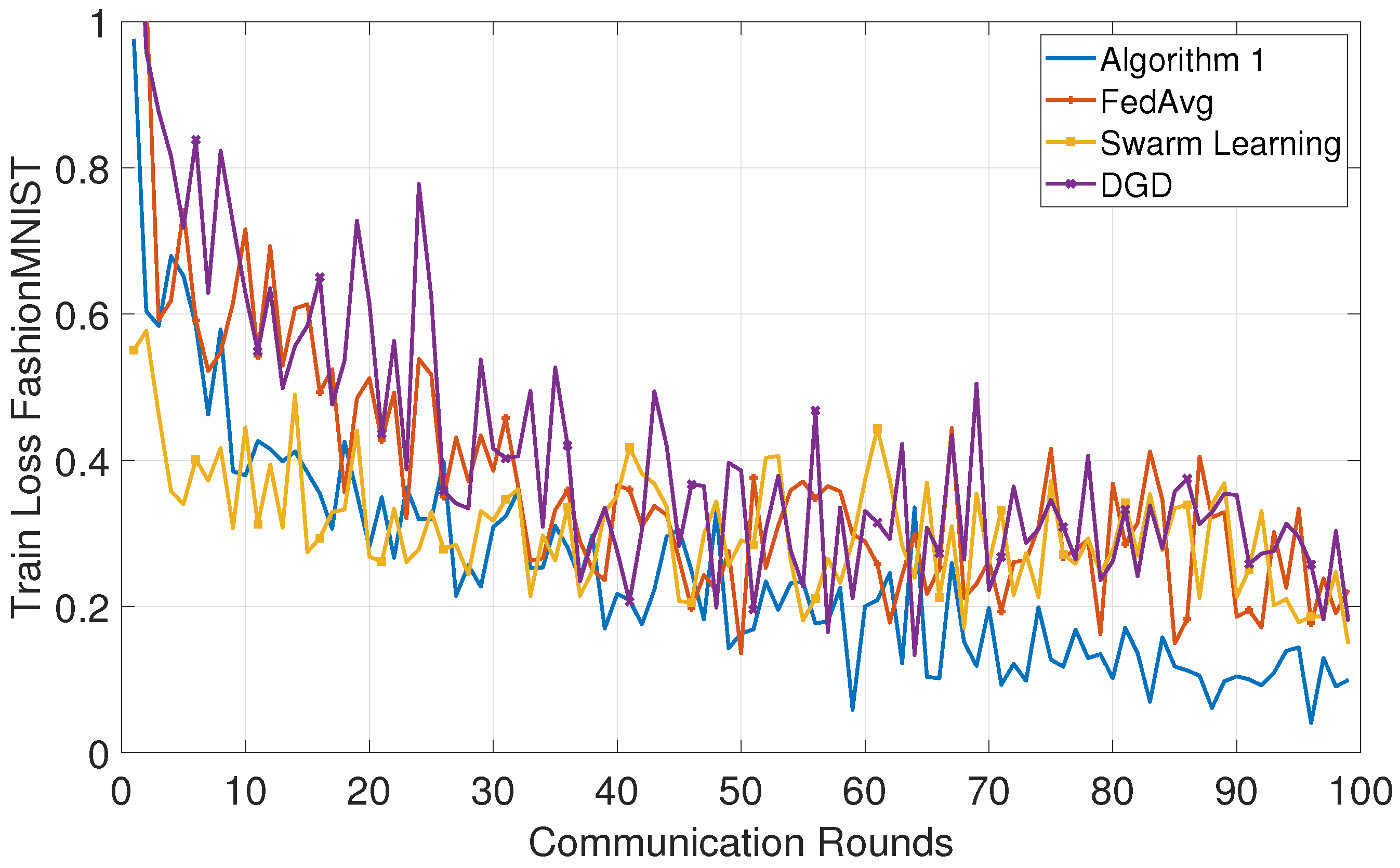
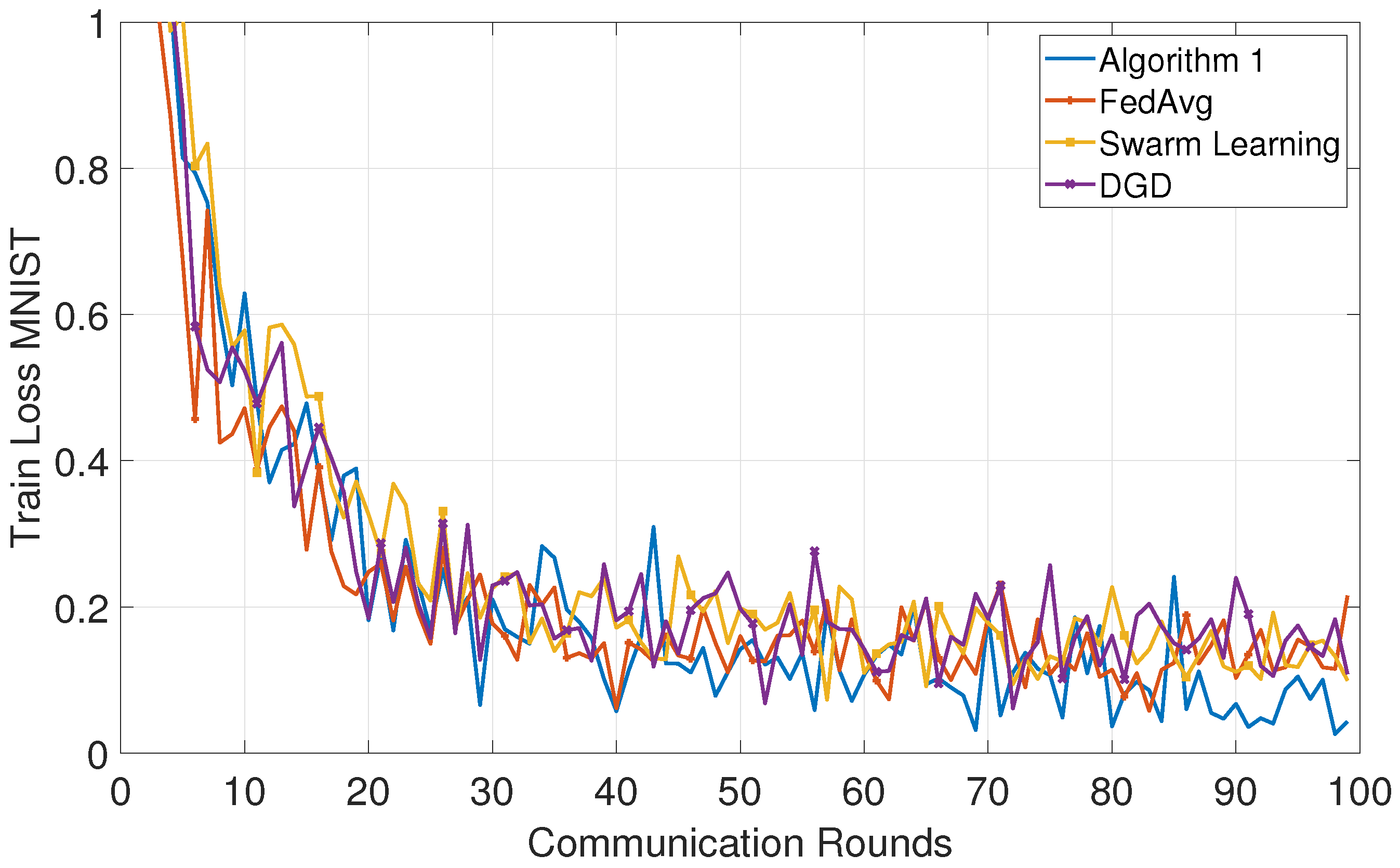
(a) The variation in model training loss across different datasets as the number of communication rounds increases is vividly illustrated in Figure 2 and Figure 3. This analysis sheds light on the dynamic behavior of the training process under varying communication scenarios. As observed, with each additional communication round, the training loss for each client consistently decreases, a testament to the iterative refinement of the models. Moreover, it is noteworthy that Algorithm 1 demonstrates a distinct advantage over other algorithms, with its clients consistently achieving lower training loss values. This suggests that Algorithm 1 is more adept at leveraging the available data and optimizing the model parameters effectively. This observation underscores the effectiveness of Algorithm 1 in achieving model convergence within a relatively small number of communication rounds.

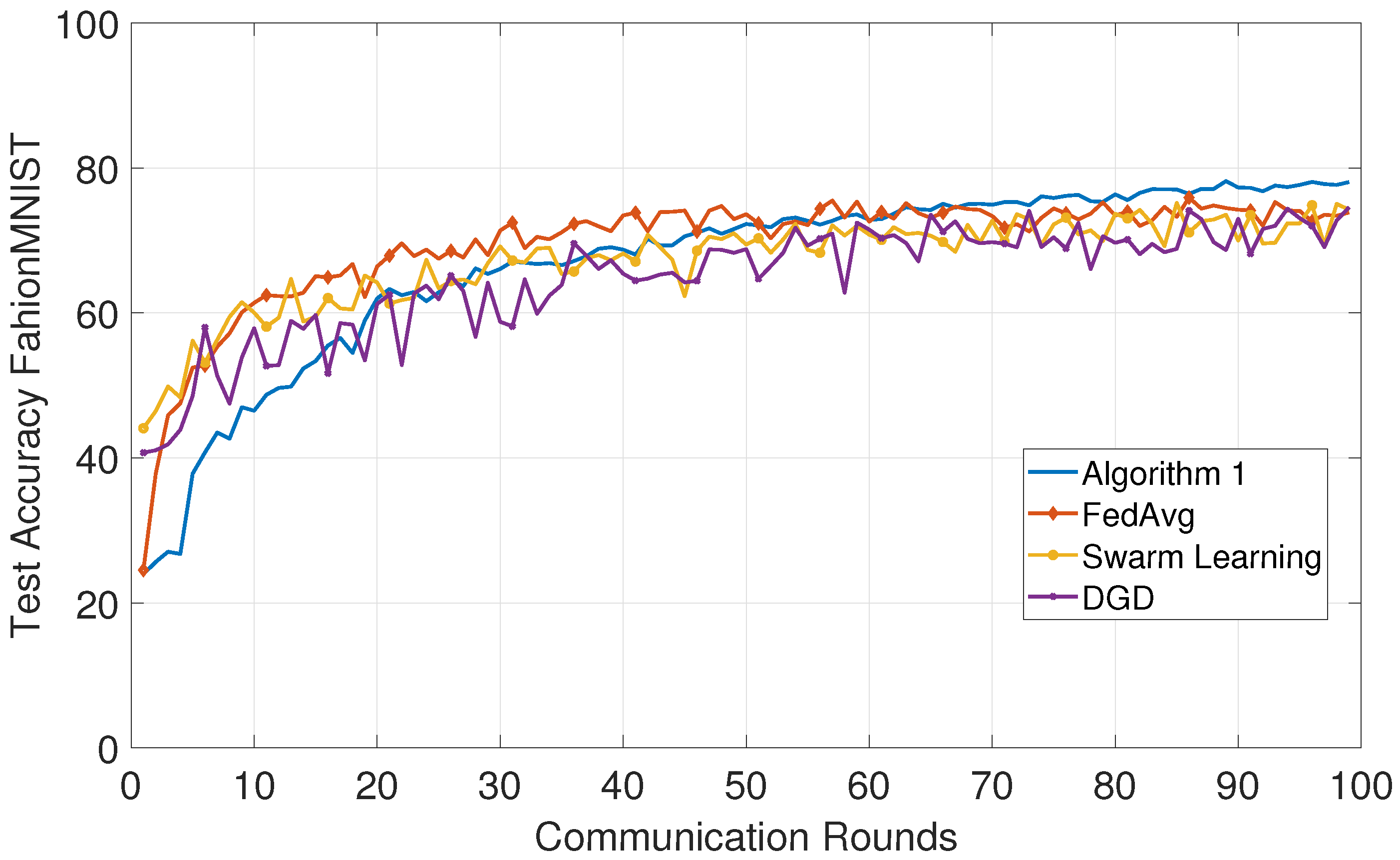
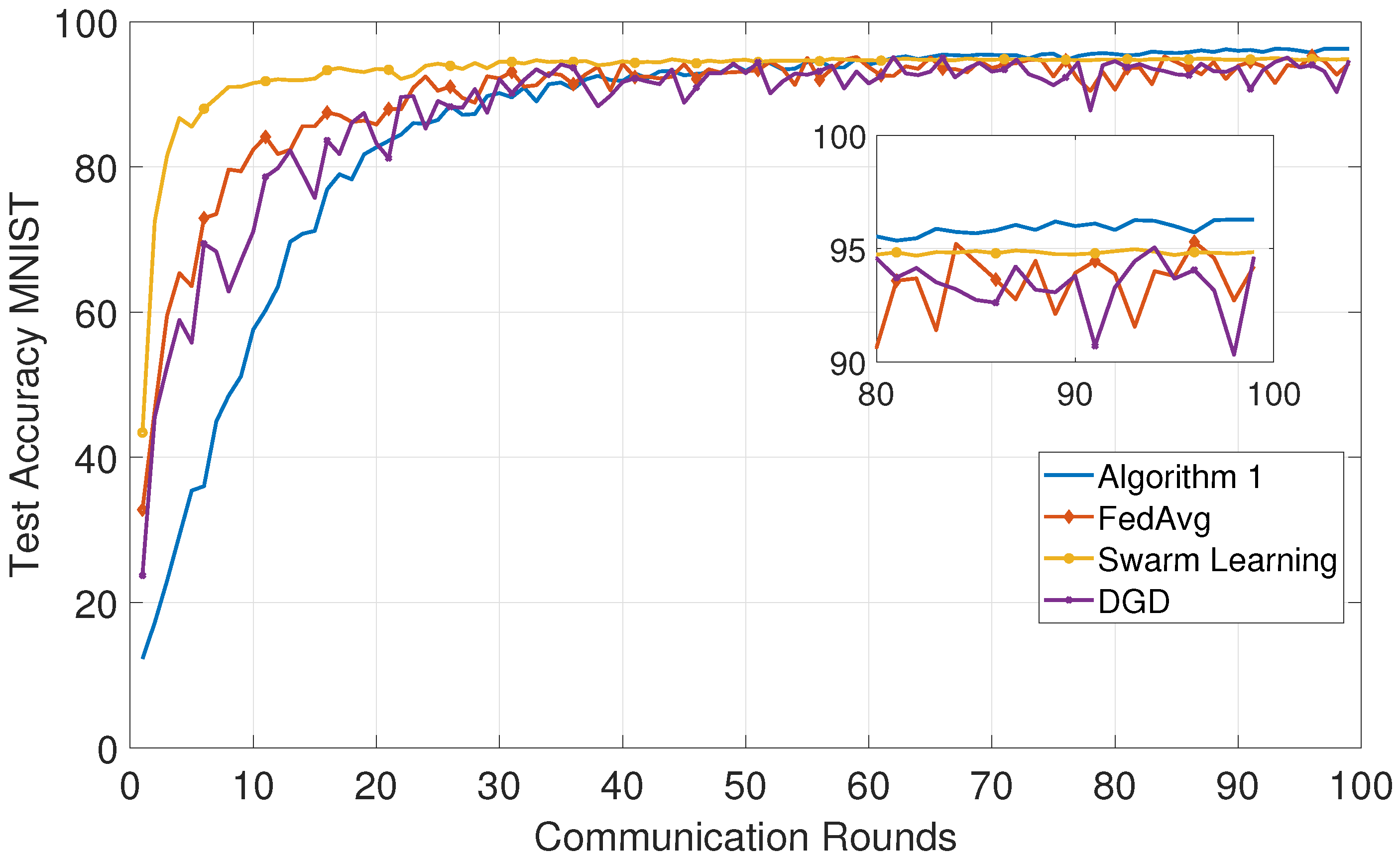
(b) The evolution of test accuracy for the four algorithms in the non-IID scenario is depicted by Figure 4 and Figure 5. Notably, Algorithm 1 exhibits a slower convergence rate yet achieves substantial test accuracy compared to alternative algorithms after several iterations. This observation highlights the algorithm’s robustness and ability to learn effectively from non-IID data distributions. Interestingly, when linear constraints are present, Algorithm 1 demonstrates accuracy akin to Swarm Learning, suggesting its adaptability to diverse constraint settings. The algorithm’s capability to conduct a linear search within the feasible domain at each step proves effective in handling constraint boundaries, ensuring that the optimization process remains efficient and effective. Operating in a fully decentralized fashion, Algorithm 1 ensures client privacy through the implementation of local differential privacy mechanisms, a crucial aspect in sensitive data environments. This dual capability underscores that Algorithm 1 can maintain high accuracy while prioritizing privacy, making it suitable for a wide range of real-world applications.

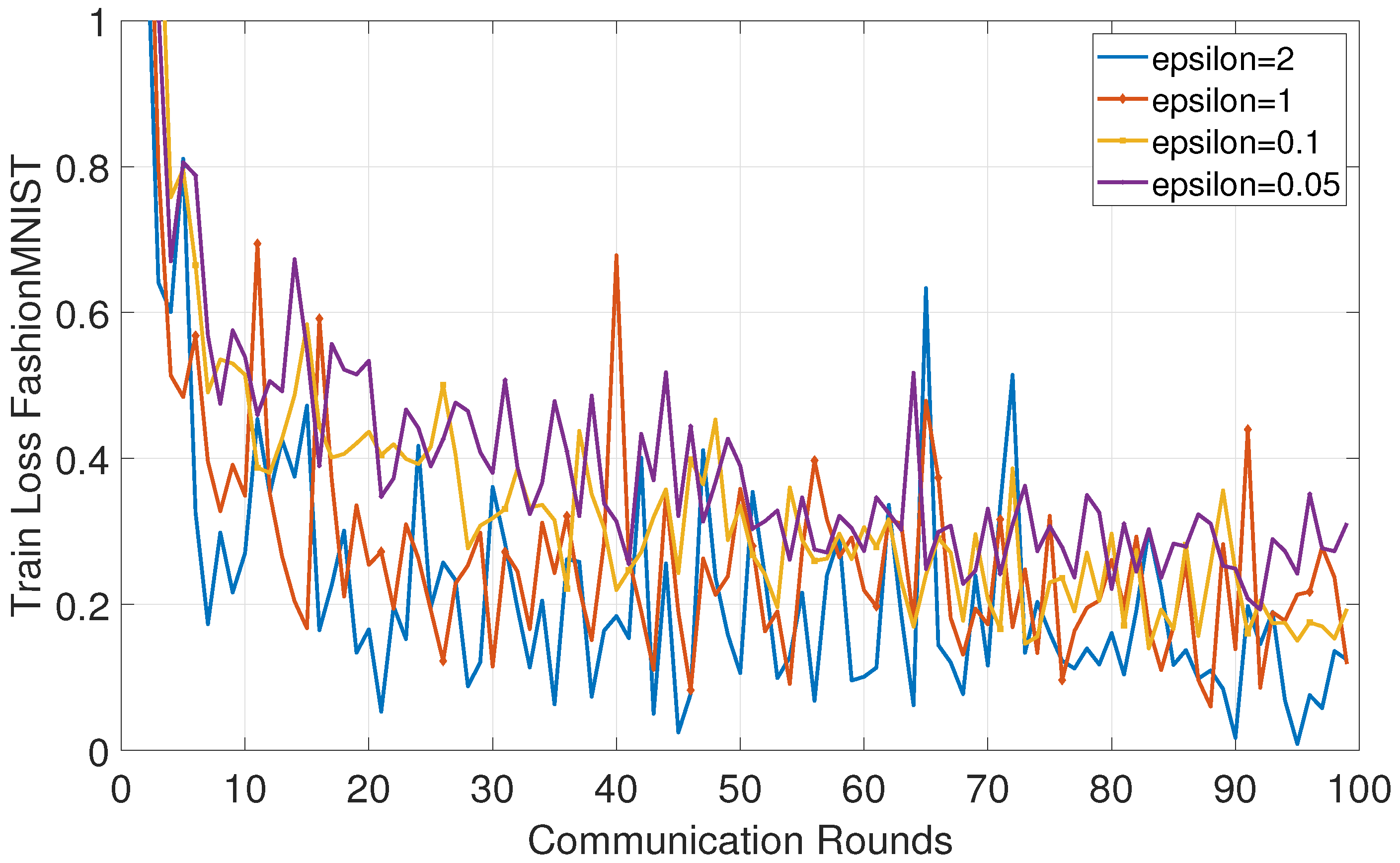
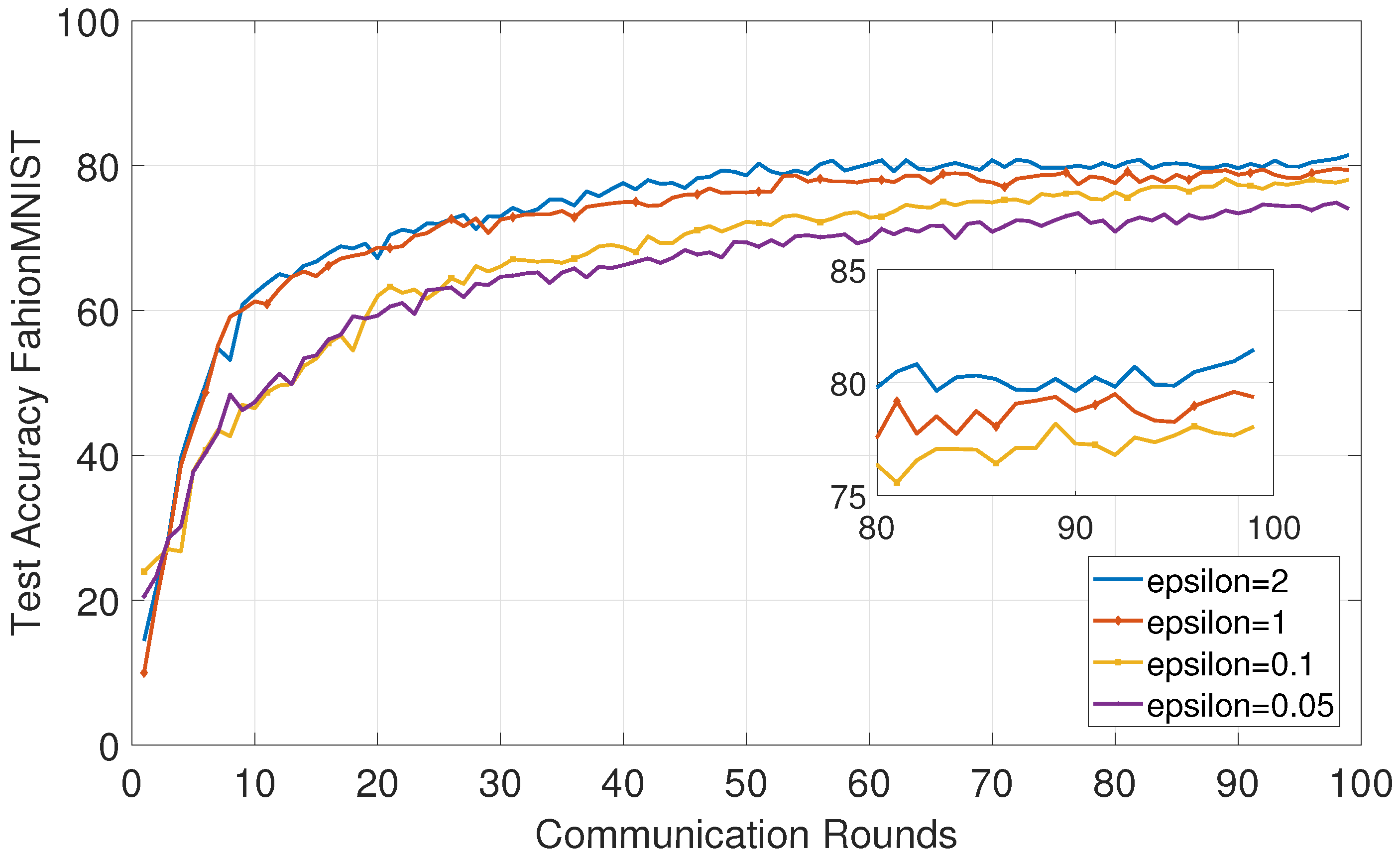
(c) In our simulation, we delve into the delicate balance between optimization accuracy and privacy budget by implementing our algorithm across different privacy budget settings. The simulation outcomes, as portrayed in Figure 6 and Figure 7, underscore a notable trend: higher privacy budgets correlate positively with enhanced accuracy and superior convergence rates. This observation not only emphasizes the critical role of adequately allocating privacy budgets but also sheds light on the pivotal relationship between privacy preservation and model performance in federated learning contexts. It suggests that prioritizing privacy measures can yield dual benefits: safeguarding sensitive data while simultaneously optimizing model efficacy. Therefore, it underscores the imperative of integrating robust privacy-preserving techniques into federated learning frameworks to ensure the attainment of both privacy objectives and model performance goals.

As shown in

Table 2. Performance comparison under different data heterogeneity levels.

Algorithm	DE = 0.85 Test Accuracy (%)	DE = 0.65 Test Accuracy (%)	DE = 0.45 Test Accuracy (%)
DPDOPFO	98.6	98.1	96.2
FedAvg	98.4	97.7	94.5
Swarm Learning	98.3	97.9	95.3
DGD	97.9	96.8	92.1

, with increasing heterogeneity from low to high (smaller DE values indicate higher data heterogeneity), the performance of all algorithms deteriorates (final accuracy decreases). As heterogeneity intensifies, the performance gap between DPDOPFO and other algorithms continues to widen. Under high heterogeneity conditions, DPDOPFO achieved a final accuracy $3.3\%$ higher than FedAvg. This demonstrates that DPDOPFO’s gradient tracking mechanism effectively mitigates the negative impact of data heterogeneity by promoting consistency in gradient estimates across clients. These results confirm that DPDOPFO maintains its relative advantage even in severe non-IID scenarios that exceed mild label bias.

(d) To validate the impact of heterogeneity on the proposed algorithm, we evaluated the performance difference between DPDOPFO and the baseline algorithm at three quantified heterogeneity levels (DE = 0.45, DE = 0.65, and DE = 0.85), as detailed in Table 2.

(e) To validate the effectiveness of the proposed algorithm in handling constrained problems and demonstrate the computational advantage of its projection-free updates, we conduct experiments on a constrained logistic regression task. The task is binary classification (digits 0 vs. 1) on the MNIST dataset under an L1-ball constraint (i.e., ${\parallel \mathbf{w}\parallel }_1\le 10$). We compare the following algorithms: DPDOPFO ($ϵ=0.1$), Differentially Private Projected Stochastic Gradient Descent (DP-PSGD, $ϵ=0.1$), non-private Projected Stochastic Gradient Descent (PSGD), and non-private Frank–Wolfe (FW). All algorithms start from the same initial point, and step sizes are tuned fairly.

Table 3. Performance and efficiency comparison on the constrained logistic regression task (MNIST binary classification, L1-ball constraint).

Algorithm	Projection	Constrained	Test Accuracy (%)	Test Loss
DPDOPFO ($ϵ=0.1$)	No	Yes	95.2	0.15
DP-PSGD ($ϵ=0.1$)	Yes	Yes	94.8	0.16
PSGD (non-private)	Yes	Yes	96.0	0.12
FW (non-private)	No	Yes	95.5	0.14

summarizes the performance and computational efficiency of each algorithm after 100 communication rounds. In terms of test accuracy and loss, DPDOPFO achieves performance close to that of the non-private FW method while guaranteeing differential privacy, and slightly outperforms DP-PSGD. This indicates that the projection-free approach can effectively optimize under constraints while preserving privacy.

(f) In order to clarify the respective roles of gradient tracking (GT) and Frank–Wolfe (FW) updates in the DPDOPFO algorithm, we conducted an ablation study under the same non-IID setting ($DE=0.5$) and privacy budget ($\epsilon =0.1$), comparing the full algorithm (DPDOPFO-full), a variant without gradient tracking (DPDOPFO-noGT), and a variant where the FW update is replaced by projected gradient descent (DPDOPFO-Proj). As shown in

Table 4. Results of ablation study comparing different variants of the proposed algorithm.

Algorithm Variant	Test Accuracy (%)	Convergence Stability	Time (s/round)
DPDOPFO-full	86.5	Stable	5.0
DPDOPFO-noGT	79.2	Unstable	5.1
DPDOPFO-Proj	85.8	Stable	8.0

, the full algorithm achieves the highest test accuracy (86.5%) with stable convergence, and the per-round running time is 5.0 s. In contrast, removing gradient tracking leads to a significant drop in accuracy (79.2%) and noticeable fluctuations in convergence, which verifies the critical role of the GT mechanism in maintaining performance and stability under data heterogeneity. The variant using projected gradient descent achieves comparable accuracy (85.8%), but its per-round running time increases to 8.0 s, which is about 60% longer than that of the full algorithm, demonstrating the computational efficiency advantage of the FW update in constrained optimization. These results clearly indicate that gradient tracking is essential for effective convergence in heterogeneous data environments, while the Frank–Wolfe update significantly improves computational efficiency without compromising accuracy.

5. Discussion

This work investigates differentially private decentralized online projection-free optimization over time-varying complex networks, and the theoretical and empirical findings suggest several implications and limitations worth discussing. First, the dynamic regret analysis reveals how the performance of the proposed DPDOPFO algorithm explicitly depends on the variation budgets of the loss functions and gradients, as well as on the mixing properties of the communication graph. In particular, the obtained regret bound shows that sublinear dynamic regret is achievable under modest assumptions on function smoothness and graph connectivity, thereby extending dynamic Frank–Wolfe-type results from centralized settings to fully decentralized federated learning architectures. This highlights that projection-free methods, when combined with gradient tracking, can achieve competitive online learning guarantees without incurring the high cost of repeated projections. Importantly, while our theoretical guarantees are derived under convexity assumptions, they provide valuable design principles for complex systems with high-dimensional constraints, data heterogeneity, and privacy requirements. Our experiments demonstrate that these principles remain effective even in non-convex neural networks.

The integration of differential privacy introduces a fundamental trade-off between privacy protection and learning accuracy. Theoretical sensitivity analysis justifies the use of Laplace noise with a privacy-budget-dependent scale, and the numerical experiments on benchmark image datasets (e.g., FashionMNIST and MNIST) demonstrate that larger privacy budgets (i.e., weaker noise) lead to faster convergence and higher accuracy, whereas stronger privacy (smaller $ϵ$) inevitably degrades performance. Nonetheless, within a practical range of $ϵ$, DPDOPFO maintains accuracy comparable to or better than representative baselines such as FedAvg, Swarm Learning, and decentralized gradient descent in non-IID settings, indicating that the algorithm can offer meaningful privacy guarantees without completely sacrificing utility in decentralized federated learning scenarios.

While the Laplace mechanism provides straightforward $(ϵ,\delta )$-DP guarantees, its utility in high-dimensional settings warrants careful consideration. Lemma 1 shows that the ${\mathsf{\ell }}_1$-sensitivity scales as ${\mathrm{\Delta }}_t\le \alpha \sqrt{d}M$, where d is the model dimension. This $\sqrt{d}$ dependence implies that the variance of the required Laplace noise grows linearly with d (since $\sigma \propto {\mathrm{\Delta }}_t\propto \sqrt{d}$). In practical federated learning scenarios with high-dimensional neural networks (e.g., $d>{10}^6$), achieving strong privacy (small $ϵ$) may necessitate noise that dominates the true gradient signal, significantly degrading learning utility. This fundamental tension between privacy and utility in high dimensions is not unique to our algorithm but represents a general challenge for DP in machine learning.

Several directions could mitigate this issue in future work. First, the Gaussian mechanism with moment accountant analysis often provides better privacy–utility trade-offs for high-dimensional queries under $(ϵ,\delta )$-DP, as it relies on ${\mathsf{\ell }}_2$-sensitivity which may be smaller than ${\mathsf{\ell }}_1$-sensitivity for gradient vectors. Second, dimensionality reduction techniques such as random projection or gradient compression (e.g., top-k sparsification) applied before noise addition can effectively reduce the sensitivity. Third, leveraging the structure of constraint sets in projection-free algorithms may offer inherent robustness to noise; for instance, the linear oracle for the ${\mathsf{\ell }}_1$-ball constraint selects only a few coordinates, potentially limiting the impact of noise across all dimensions. Exploring these alternatives within our decentralized framework would be valuable for scaling privacy-preserving federated learning to very high-dimensional models.

Furthermore, while our experimental evaluation focuses on unconstrained neural network training for benchmark comparison, the computational advantages of the projection-free Frank–Wolfe approach become particularly pronounced when dealing with complex constraint sets. The experimental results underline the role of network topology and gradient tracking in coping with heterogeneity across clients. Operating over time-varying directed graphs, DPDOPFO exploits local consensus and gradient tracking to reduce disagreement among agents and to follow the global gradient more accurately, which is crucial when data distributions are highly non-IID and communication links are imbalanced or intermittent. From the perspective of complex systems and complex networks, this suggests that appropriately designed mixing matrices and sufficiently frequent information exchange can partially compensate for data heterogeneity and noise injection, thereby stabilizing training and improving robustness in decentralized learning over large-scale multi-agent networks. The Laplace mechanism employed in this work for providing LDP guarantees relies on a noise scale that depends on the sensitivity. As shown in Lemma 1, the upper bound of the sensitivity grows with the square root of the model dimension d (i.e., ${\mathrm{\Delta }}_t\propto \sqrt{d}$). This implies that in high-dimensional problems, achieving the same level of privacy requires injecting a larger amount of noise, which may more significantly degrade model utility. Future work could explore noise mechanisms better suited to high-dimensional spaces, such as adopting the Gaussian mechanism combined with the moments accountant for tighter privacy accounting, or designing projection-based noise techniques that leverage the structural properties of the constraint set, so as to achieve a better privacy–utility trade-off under strict privacy protection.

Despite these advantages, several limitations remain. The current analysis is restricted to convex and smooth loss functions with compact constraint sets and relies on synchronous updates and idealized local computation. Real-world deployments may involve non-convex deep models, asynchronous or event-triggered communication, time-varying participation of clients, and more structured constraints (e.g., low-rank or sparsity-inducing sets) that may alter both the regret behavior and the privacy–utility trade-off. Furthermore, only Laplace-based local differential privacy is considered; exploring alternative mechanisms (e.g., Gaussian mechanisms, Rényi differential privacy, or adaptive noise schedules) and their impact on dynamic regret and empirical performance is an important direction for future research. Finally, applying DPDOPFO to domain-specific complex systems—such as industrial IoT, smart grids, or large-scale cyber–physical infrastructures—will require additional considerations on system-level reliability, communication overhead, and secure deployment, which go beyond the scope of the present simulation-based evaluation.

6. Conclusions

This paper investigates the problem of privacy-preserving distributed online convex optimization in time-varying unbalanced networks. To address the challenges associated with the costly computation of projections onto high dimensional complex constraint sets, we propose a distributed online Frank–Wolfe algorithm based on differential privacy techniques. In this algorithm, each agent collaboratively minimizes the global cost function through local exchanges with neighbors on the time-varying network. Theoretical analysis indicates that the algorithm achieves sublinear regret while preserving privacy, elucidating the relationship between privacy levels and accuracy. The algorithm’s effectiveness is validated through comprehensive simulation experiments. Future research directions include enhancing regret bounds, addressing scenarios with more complex constraints, extending results to non-convex and non-smooth functions, and exploring applications in other domains.