Data-Driven Probabilistic Wind Power Forecasting and Dispatch with Alternating Direction Method of Multipliers over Complex Networks

Abstract

This paper proposes a privacy-preserving framework that couples probabilistic wind power forecasting with decentralized anomaly detection in complex power networks. We first design an adaptive federated learning (FL) scheme to produce probabilistic forecasts for multiple geographically distributed wind farms while keeping their raw data local. In this scheme, an artificial neural network with quantile regression is trained collaboratively across sites to provide calibrated prediction intervals for wind power outputs. These forecasts are then embedded into an alternating direction method of multipliers (ADMM)-based load-side dispatch and anomaly detection model for decentralized power systems with plug-and-play industrial users. Each monitoring node uses local measurements and neighbor communication to solve a distributed economic dispatch problem, detect abnormal load behaviors, and maintain network consistency without a central coordinator. Experiments on the GEFCom 2014 wind power dataset show that the proposed FL-based probabilistic forecasting method outperforms persistence, local training, and standard FL in RMSE and MAE across multiple horizons. Simulations on IEEE 14-bus and 30-bus systems further verify fast convergence, accurate anomaly localization, and robust operation, indicating the effectiveness of the integrated forecasting–dispatch framework for smart industrial grids with high wind penetration.

1. Introduction

Wind energy, as a vital renewable source, plays an increasingly significant role in decentralized power systems. However, its inherent intermittency and volatility pose considerable challenges to grid operation, including power quality degradation, reduced system reliability, and increased spinning reserve requirements. Therefore, accurate Wind Power Forecasting (WPF) is critical. On the one hand, wind energy can provide clean and high-quality energy to load centers; on the other hand, a high penetration of wind power increases the regional grid’s dependence on external high-power sources [1].

The decentralized power system is a complex network structure that connects distributed production units and provides electrical power services to various industrial terminals. Unlike traditional large power grids [2], the distributed production and consumption units in industrial supply chains have plug-and-play characteristics, but this also leads to more complex dynamic properties, making their anomaly detection more complicated. With the proliferation of smart power electronic devices, industrial terminals in the supply chain are becoming more diverse and sophisticated, and any power consumption anomalies can have significant impacts. Reference [3] proposed a genetic algorithm, reference [4] achieved a hybrid optimization solution by combining evolutionary algorithms and sequential quadratic programming, and references [5,6] utilized particle swarm optimization to design algorithms for finding the optimal anomaly detection solution. Traditional WPF primarily focuses on providing a single-point estimate of the wind power output for a specific future timestamp, known as Deterministic WPF. This approach typically relies on advanced time series models or neural networks (such as Recurrent Neural Networks (RNNs) [7], Long Short-Term Memory (LSTM) [8], or Convolutional Neural Networks (CNNs)) [9] to capture spatiotemporal dependencies and enhance prediction accuracy. However, due to wind power’s strong dependence on meteorological factors (e.g., wind speed, direction, temperature) and the chaotic nature of weather systems, deterministic forecasting fundamentally fails to capture the inherent stochastic uncertainty in wind power generation. A single-value prediction severely limits its utility in risk-sensitive power system decisions, such as grid security analysis and reserve capacity allocation. To overcome the limitations of deterministic forecasting, Probabilistic WPF has emerged [10]. Instead of seeking a single optimum value, it provides a prediction of the output along with an associated estimation of uncertainty [11]. This uncertainty information is typically presented in the form of a set of quantiles, Prediction Intervals (PIs), or a complete Probability Density Function (PDF). Probabilistic forecasts, which explicitly include risk information, are indispensable for generation scheduling optimization, electricity market trading risk management, and grid planning. For instance, grid operators utilize PIs to set more reasonable reserve capacities, thereby reducing operating costs and ensuring supply reliability.

Furthermore, with the increasing scale of distributed wind farms and the rising concern for data privacy, Federated Learning (FL) has emerged as a novel paradigm to enhance WPF [12]. Unlike traditional centralized training, where data from all wind farms must be aggregated to a central server, FL enables multiple local wind farms to collaboratively train a shared prediction model [13,14,15]. Each local farm trains the model using its private data and only shares the model updates (gradients) with the central server. This approach effectively enhances forecasting accuracy by leveraging the diverse data distribution across the fleet, while rigorously ensuring that sensitive local operational data remains on the wind farm’s premises, addressing critical privacy and communication bandwidth concerns inherent in large-scale decentralized systems [16]. Traditional anomaly detection optimization algorithms still have many drawbacks. The algorithms in references [3,4,5,6,17,18] all require a control center for centralized anomaly identification, which is very unsuitable for the capacity of today’s large industrial supply chains, especially since some areas with distributed industrial users are remote and difficult to monitor centrally. Moreover, the industrial supply chain can be viewed as a complex network system, where production and consumption units can be seen as nodes in this complex network [19]. Therefore, using a distributed consensus optimization strategy that relies solely on local information transmission is a good approach to solving the anomaly detection problem. In references [20,21,22,23], controllers based on multi-agent consensus design are discussed, where neighboring agents can exchange their information to achieve optimal anomaly identification consensus.

Multi-agent anomaly detection problems can be divided into continuous-time and discrete-time algorithms, both of which have been extensively studied [24,25,26,27]. In fact, consistency has always been one of the foundations of multi-agent systems, and with the application of intelligent monitoring nodes, these algorithms have also been gradually applied to industrial power anomaly detection [28,29,30]. Although these studies have promoted the development of anomaly detection in industrial supply chains, some drawbacks still exist. Some anomaly detection problems with capacity constraints cannot be well addressed, as shown in the literature [31,32], which can only solve problems with power consumption balance equality constraints. On this basis, the literature [33] theoretically solved for the first time the relationship between state consistency and optimal anomaly detection solutions, establishing a fundamental normative framework for industrial power anomaly monitoring.

Beyond smart grids, there has been growing interest in the resilience and security of other large-scale networked infrastructures, such as complex traffic systems and industrial Internet of Things (IIoT) platforms. For example, resilience recovery methods based on trend forecasting have been proposed for complex traffic network security [34], and interpretable deep learning frameworks have been developed for intrusion detection in industrial IoT environments [35]. These studies share with our work the common goal of ensuring secure and reliable operation of cyber–physical systems under uncertainty and potential attacks. From a methodological perspective, our adaptive FL framework, which combines Adaptive Clustering (AC) and Elastic Weight Consolidation (EWC), is also conceptually related to recent advances in adaptive sparse memory networks for efficient and robust sequence and video modeling [36]. Incorporating similar sparse and dynamically allocated memory mechanisms into federated probabilistic forecasting models is an interesting direction for future improvements in both computational efficiency and robustness.

This paper conducts an in-depth analysis of anomaly detection and monitoring issues that may arise in upstream and downstream industrial power systems. When abnormal power consumption patterns occur, utilizing the characteristics of intelligent monitoring nodes and based on anomaly detection theory, power anomaly identification is directly performed from the load side, allowing the monitoring system to quickly and effectively identify abnormal states without interference. This short-term distributed anomaly detection plan has minimal impact on industrial users, and monitoring equipment can operate at low power consumption. A rigorous mathematical proof is also provided, ultimately demonstrating that the anomaly detection parameters can converge to an ideal value, minimizing the economic losses caused by undetected anomalies to the industrial power system. From a modelling perspective, our probabilistic forecasting framework is fundamentally different from recent information-/physics-embedded approaches such as the physics-embedding multi-response regressor for time-variant system reliability assessment in [37]. The model in [37] is designed for complex engineering systems whose behaviour can be described by detailed physics-based models and multiple time-variant performance functions. By transforming time-variant responses into time-invariant extreme-value representations and embedding physics and mathematical knowledge into a multi-response surrogate, it achieves high accuracy and sample efficiency for reliability assessment under rich physics information. While the physics-embedded regressor in [37] is highly suitable when detailed physical models and multi-response reliability indicators are available, our federated probabilistic model is better aligned with the requirements of short-term wind power forecasting and distributed grid operation considered in this paper, where scalability across many wind farms, communication efficiency, and compliance with data-governance constraints are of primary concern.

2. Preliminaries and Network Model

2.1. LSTM Networks

In this work, we adopt a standard LSTM-based time-series forecasting pipeline for each wind farm. The raw wind power measurements are first aligned in time, cleaned, and normalized. Then, for each wind farm, we construct input–output pairs by sliding a fixed-length window over the historical time series: a sequence of past measurements is used as input, and the subsequent values over a given prediction horizon are used as targets. The LSTM network processes the input sequence and outputs the forecasted wind power (or quantiles thereof), and the model parameters are trained by minimizing an appropriate loss function on the training set. This LSTM-based forecaster serves as the local prediction model within the federated learning framework described in Section 3.

The univariate time series is reframed into input-output (Input-Output, ${\mathcal{S}}_t$) sequence pairs suitable for supervised learning. This is achieved via a fixed-length sliding window mechanism, which defines the look-back window $T_{\mathrm{in}}$ (input sequence length) and the forecast horizon $T_{\mathrm{out}}$ (prediction sequence length):

$${\mathcal{S}}_t=({\mathbf{X}}_t,{\mathbf{Y}}_t)$$

(1)

where the input feature sequence ${\mathbf{X}}_t\in {\mathbb{R}}^{T_{\mathrm{in}}\times d}$ comprises d dimensional features over the preceding $T_{\mathrm{in}}$ time steps, and the target sequence ${\mathbf{Y}}_t\in {\mathbb{R}}^{T_{\mathrm{out}}\times k}$ contains the k-dimensional prediction targets for the subsequent $T_{\mathrm{out}}$ steps.

Model optimization is realized by minimizing a predefined Loss Function, such as the Mean Squared Error (MSE) for deterministic forecasting or Pinball Loss for probabilistic forecasting, utilizing backpropagation through time (BPTT). Upon obtaining the model’s projected output, an inverse normalization transformation is executed to restore the predicted values to their original physical units. Following this transformation, the model’s performance is rigorously assessed using standard metrics like the Root Mean Square Error (RMSE) or Mean Absolute Error (MAE).

The fundamental innovation of the LSTM unit lies in its dedicated Cell State (${\mathbf{C}}_t$), which functions as a linear pathway capable of carrying information across extended time steps without degradation. The flow of information along this state is meticulously controlled by three distinct gate structures. Each gate operates as a soft switch, implemented via the Sigmoid function ($\sigma$) and a learned weight matrix, producing a signal in the range of $[0,1]$.

At each time step t, the computation within the LSTM unit is a composite function of the previous hidden state ${\mathbf{h}}_{t-1}$, the previous cell state ${\mathbf{C}}_{t-1}$, and the current input ${\mathbf{x}}_t$. Forget Gate (Regulator of Past Information): The forget gate computes its activation based on the concatenated previous hidden state and current input.

$${\mathbf{f}}_t=\sigma ({\mathbf{W}}_f·[{\mathbf{h}}_{t-1},{\mathbf{x}}_t]+{\mathbf{b}}_f)$$

(2)

Input Gate and Candidate Memory (Regulator of New Information): The input gate ${\mathbf{i}}_t$ scales the relevance of the new candidate memory ${\tilde{\mathbf{C}}}_t$, which proposes the new information to be stored in the cell state.

$${\mathbf{i}}_t=\sigma ({\mathbf{W}}_i·[{\mathbf{h}}_{t-1},{\mathbf{x}}_t]+{\mathbf{b}}_i)$$

(3)

$${\tilde{\mathbf{C}}}_t=tanh({\mathbf{W}}_C·[{\mathbf{h}}_{t-1},{\mathbf{x}}_t]+{\mathbf{b}}_C)$$

(4)

Cell State Update (The Linear Highway): The cell state is updated by selectively forgetting old information (scaled by ${\mathbf{f}}_t$) and adding new filtered information (scaled by ${\mathbf{i}}_t$). The additive nature of this update is the mechanism that ensures an unobstructed path for the gradient, thereby mitigating the vanishing gradient issue.

$${\mathbf{C}}_t={\mathbf{f}}_t\odot {\mathbf{C}}_{t-1}+{\mathbf{i}}_t\odot {\tilde{\mathbf{C}}}_t(\mathrm{Cell}\mathrm{State}\mathrm{Update})$$

(5)

Output Gate and Hidden State (Unit Output): The output gate ${\mathbf{o}}_t$ controls the flow of information from the cell state ${\mathbf{C}}_t$ to the hidden state ${\mathbf{h}}_t$, which serves as the unit’s output and input for the subsequent time step.

$${\mathbf{o}}_t=\sigma ({\mathbf{W}}_o·[{\mathbf{h}}_{t-1},{\mathbf{x}}_t]+{\mathbf{b}}_o)$$

(6)

$${\mathbf{h}}_t={\mathbf{o}}_t\odot tanh\left({\mathbf{C}}_t\right)(\mathrm{Hidden}\mathrm{State})$$

(7)

where ${\mathbf{W}}_{*}$ and ${\mathbf{b}}_{*}$ are the learned weight matrices and bias vectors for each gate and candidate memory, respectively. $\sigma \left(·\right)$ donotes the Sigmoid activation function, $\sigma \left(z\right)=1/(1+e^{-z})$ and $tanh\left(·\right)$ represents the Hyperbolic Tangent activation function, normalizing values to $[-1,1]$. ⊙ is the Hadamard product (element-wise multiplication), enabling the gating control and $[{\mathbf{h}}_{t-1},{\mathbf{x}}_t]$ denotes vector concatenation.

This precise algebraic construction empowers the LSTM to effectively manage information flow over long sequences, granting it superior stability and predictive accuracy compared to conventional RNN architectures in time series modeling.

2.2. Optimization Theory of ADMM

The standard form of the ADMM algorithm is used to solve the following problem:

$$\begin{array}{cc}\hfill & \underset{x_1,x_2}{min}f\left(x_1\right)+f\left(x_2\right)\hfill \\ \mathrm{s}.\mathrm{t}.\hfill & A_1{x}_1+A_2{x}_2=d\hfill \end{array}$$

(8)

In the expression, the variables $x_1\in {\mathbb{R}}^n,x_2\in {\mathbb{R}}^n$, the constant matrices $A_1\in {\mathbb{R}}^{p\times n},A_2\in {\mathbb{R}}^{p\times m}$, and the constant $d\in {\mathbb{R}}^n$ must all be in full rank status to ensure that the problem has a feasible solution. For the problem (8), using the augmented Lagrange multiplier method, we can obtain:

$$\begin{array}{cc}\hfill {\mathcal{L}}_{\rho }\left(x_1,x_2,\lambda \right)& =f\left(x_1\right)+g\left(x_2\right)+z^{\mathrm{T}}\left(A_1{x}_1+A_2{x}_2-d\right)\hfill \\ \hfill & +(\rho /2){∥A_1{x}_1+A_2{x}_2-d∥}_2^2\hfill \end{array}$$

(9)

In the formula, z is the Lagrange multiplier corresponding to the equality constraint $A_1{x}_1+A_2{x}_2=d$, while the penalty factor $\rho$ is an artificially set positive scalar.

For fixed $x_2^k$ and ${\lambda }^k$, the update of $x_1$ is obtained by minimizing the augmented Lagrangian with respect to $x_1$:

$$\begin{array}{cc}\hfill x_1^{k+1}& =arg\underset{x_1}{min}{L}_{\rho }(x_1,x_2^k,{\lambda }^k)\hfill \\ \hfill & =arg\underset{x_1}{min}\left\{f\left(x_1\right)+{\left({\lambda }^k\right)}^{\top }(A_1{x}_1+A_2{x}_2^k-d)+{\displaystyle \frac{\rho }{2}}{∥A_1{x}_1+A_2{x}_2^k-d∥}_2^2\right\}.\hfill \end{array}$$

(10)

Dropping the terms that do not depend on $x_1$, the subproblem reduces to a convex optimization problem in $x_1$ only. The update $x_1^{k+1}$ is thus given by the first line of the ADMM iteration. Similarly, for fixed $x_1^{k+1}$ and ${\lambda }^k$, the update of $x_2$ is

$$\begin{array}{cc}\hfill x_2^{k+1}& =arg\underset{x_2}{min}{L}_{\rho }(x_1^{k+1},x_2,{\lambda }^k),\hfill \end{array}$$

(11)

which yields the second line of the ADMM iteration. Finally, the dual variable is updated by a gradient ascent step on the dual function,

$$\begin{array}{c}\hfill {\lambda }^{k+1}={\lambda }^k+\rho \left(A_1{x}_1^{k+1}+A_2{x}_2^{k+1}-d\right),\end{array}$$

(12)

which enforces the equality constraint $A_1{x}_1+A_2{x}_2=d$ over iterations.

2.3. Wind Power Dispatch Model

Considering the wind power system model of a total of $n,n=1,2,3\dots$ loads, all of which are controllable loads. When a sudden event occurs, the power of the generation unit suddenly decreases by $▵p$, and at the same time, the overall frequency will also drop. The rated frequency of the grid system is defined as ${\omega }^{*}$. It is assumed that each load monitors its frequency variation and adjusts its load demand amount during each time interval $▵t$. For convenience, let $t=0,1,2\dots$ represent the time interval $t=\Delta t,2\Delta t\dots$. When encountering a sudden event, the frequency of the entire system will experience a relative drift from ${\omega }^{*}$, where the overall global frequency deviation of the smart grid is defined in an ideal state. Next, we define the local frequency deviation value $▵\overline{{\omega }^{*}}$ measured by the sensor of the agent at the $i^{th}$ load. The difference from the global frequency deviation $▵\omega$ lies in inconsistencies caused by measurement noise $v_i$. Due to the differences in load types, the degree of noise interference can also vary. $▵P_g$ represents the power reduction at the generation end caused by an incident, and to maintain supply-demand balance, load i needs to reduce its own power consumption $▵P_{li}$ accordingly to compensate for the loss at the generation end, with specific scheduling strategies to be analyzed in detail in subsequent algorithms discussed. The supply-demand imbalance error at time t can be expressed as:

$$u\left(t\right)\triangleq \Delta P_g-\sum _{i=1}^n\Delta P_{li}$$

(13)

In order to maintain generality, under the condition that it conforms to the actual wind power system model and that the algorithm has a feasible solution, we assume that the following conditions are met during this wind power system model process:

$$\begin{array}{cc}\hfill & \Delta P_g>0\hfill \\ \hfill & \Delta P_{li}>0\hfill \end{array}$$

(14)

In order to simplify the notation, we use $p_i$ to represent $\Delta P_{li}$ in the following article. In the following, we first need to forecast the power $\Delta P_g$ generated by wind.

3. Algorithm Design

3.1. Probabilistic Wind Power with FL

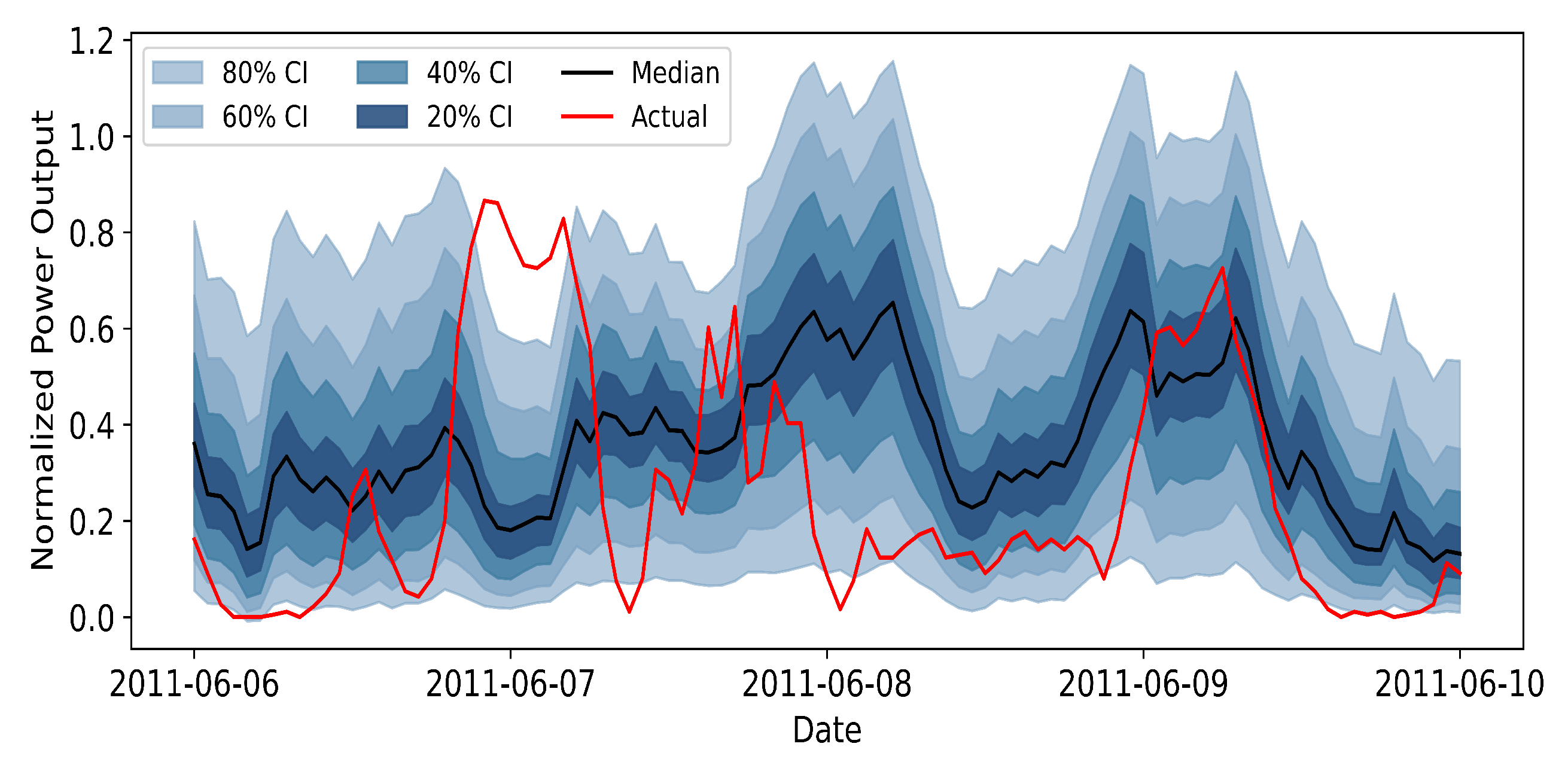
To generate probabilistic wind power forecasts in a privacy-preserving manner, we adopt an adaptive federated learning framework that couples a local quantile regression model with two mechanisms designed for Non-IID data and knowledge retention. At each communication round, every wind farm trains a local artificial neural network (ANN) with quantile regression loss on its own data and sends model updates to a server or cluster center without sharing raw measurements. The server aggregates these updates within clusters of clients that exhibit similar learning behaviour, as determined by an Adaptive Clustering (AC) strategy, and maintains a separate global model for each cluster. After global aggregation, each client performs a personalized fine-tuning step regularized by Elastic Weight Consolidation (EWC), which discourages large deviations of parameters that are important for the cluster-level model. This combination of FL, AC, and EWC yields cluster-specific global models and personalized local models that jointly provide calibrated probabilistic forecasts while respecting data locality.

Probabilistic WPF methods are broadly categorized into two main approaches, i.e., parametric and non-parametric. Parametric methods assume that the wind power error follows a predefined probability distribution and then predict the parameters of that distribution. Non-parametric methods learn the uncertainty directly from data without assuming a specific distribution form, such as Kernel Density Estimation (KDE) and Quantile Regression (QR). Within deep learning models, Quantile Regression is widely adopted due to its directness, flexibility, and minimal assumptions regarding the data distribution.

In Quantile Regression, the model is trained by minimizing the Pinball Loss (also known as Quantile Loss or Check Loss). This minimization ensures that the predicted quantile ${\widehat{y}}_{q_m,t}$ precisely splits the actual value $y_t$ into proportions $q_m$ and $1-q_m$. The definition of the Pinball Loss $l_{q_m}$ clearly demonstrates the asymmetric penalty mechanism for overestimation and underestimation:

$$l_{q_m}({\widehat{y}}_{q_m,t},y_t)=\left\{\begin{array}{cc}(1-q_m)({\widehat{y}}_{q_m,t}-y_t)\hfill & \mathrm{if}{\widehat{y}}_{q_m,t}\ge y_t\hfill \\ q_m({\widehat{y}}_{q_m,t}-y_t)\hfill & \mathrm{if}{\widehat{y}}_{q_m,t}<y_t\hfill \end{array}\right.$$

(15)

Here, $q_m$ is the target quantile, typically ranging from $0.1,0.2,\dots ,0.9$ to cover various confidence levels required for the prediction interval. When the prediction ${\widehat{y}}_{q_m,t}$ is less than the actual value $y_t$, the loss is weighted by $q_m$; conversely, it is weighted by $1-q_m$. This asymmetric penalty ensures that the model learns the ${\widehat{y}}_{q_m,t}$ value that is indeed the $q_m$-th quantile point of the data distribution. The overall training objective is to minimize the average loss across all quantiles, defined as the local loss $L_{\mathrm{local}}$. For a dataset with m quantiles and $T_i$ samples, the total average loss $L_{\mathrm{local}}$ is:

$$L_{\mathrm{local}}({\widehat{y}}_i,y_i)={\displaystyle \frac{1}{m{T}_i}}\sum _{t=0}^{T_i-1}\sum _{d=0}^{m-1}{l}_{q_d}({\widehat{y}}_{q_d,t},y_t)$$

(16)

This comprehensive loss function guides the neural network training to output predictions that simultaneously satisfy the requirements of multiple quantiles.

To address the Non-IID nature of local datasets across wind farms, we introduce an adaptive clustering procedure that groups clients with similar preference scores and jointly trains a cluster-specific global model. Within each cluster, model parameters are aggregated in a federated manner to capture shared patterns among the corresponding wind farms. Furthermore, elastic weight consolidation (EWC) is employed during local personalization to preserve important global knowledge: parameters that are estimated to be critical for the global model are penalized if they deviate too much from their global values, which mitigates catastrophic forgetting while still allowing client-specific adaptation.

The purpose of the AC strategy is to automatically identify and separate clients with similar model learning characteristics and data distributions without exposing raw data. These clients are assigned to distinct clusters $C_j$, and a customized global model $M_j^g$ is trained for each cluster. The detailed steps are as follows.

Warm-up Training: The server initializes k models $M_j^g$ and distributes them to all clients. Each client trains these k models locally for a small number of epochs (e.g., $P_w$ rounds) using the local loss $L_{\mathrm{local}}$. This stage is designed to help clients move past initialization randomness and establish stable, distinguishable preferences for the k models.

Preference Score Update: During the clustering phase, clients no longer update all k models. Instead, they use the performance $e_{i,j}^{\left(p\right)}$ (Pinball Loss) of the k models on their local validation set to update the preference score $s_{i,j}^{\left(p\right)}$. The model yielding the best performance is deemed the client’s favorite. The decay rate $\beta \in [0,1]$ controls the influence of historical preferences.

$$\left\{\begin{array}{cc}{s}_{i,j}^{\left(p\right)}=\beta s_{i,j}^{(p-1)}+1\hfill & \mathrm{if}{e}_{i,j}^{\left(p\right)}={\widehat{e}}_i^{\left(p\right)}\hfill \\ s_{i,j}^{\left(p\right)}=s_{i,j}^{(p-1)}\hfill & \mathrm{if}{e}_{i,j}^{\left(p\right)}>{\widehat{e}}_i^{\left(p\right)}\hfill \end{array}\right.$$

(17)

Intra-Cluster Aggregation: The server receives the parameters ${\tilde{M}}_i^l$ of the client’s favorite model. Based on the model index ${\tilde{k}}_i$, the client is assigned to the corresponding cluster $C_j$. Aggregation is performed only within the cluster to prevent gradient conflicts arising from severe data heterogeneity between different clusters. The clustering process terminates when the client preferences $\tilde{k}=\left\{{\tilde{k}}_i\right\}$ remain unchanged for $E_A$ consecutive epochs, ensuring stability of the clustering result.

Elastic Weight Consolidation (EWC) first identifies which global parameters $w_h^g$ are critical to the overall global model performance. It uses a diagonal approximation of the Fisher Information Matrix to calculate the importance $I_{i,h}$ for each model parameter $w_{i,h}^l$. This value is based on the average of the squared first-order derivatives (gradients) of the local loss function $L_{\mathrm{local}}$ with respect to the parameter on the local dataset $D_i$:

$$I_{i,h}\approx {\displaystyle \frac{1}{|D_D|}}\sum _{x\in D_i}{\left({\displaystyle \frac{\partial L_{\mathrm{local}}}{\partial w_{i,h}^l}}\right)}^2$$

(18)

A higher $I_{i,h}$ value indicates that the parameter is more critical for the model’s core feature extraction capabilities, and thus should be more strictly protected during fine-tuning. EWC Loss Function: During personalized fine-tuning, the EWC Loss function $L_{\mathrm{EWC}}$ is used. It supplements the original local loss $L_{\mathrm{local}}$ with a regularization term. This term penalizes the parameter $w_{i,h}^l$ for deviating too far from the initial global model parameter $w_h^g$, scaled by its importance $I_{i,h}$:

$$L_{\mathrm{EWC}}=L_{\mathrm{local}}+\gamma \sum _{h=0}^{|W^l|-1}{I}_{i,h}{(w_{i,h}^l-w_h^g)}^2$$

(19)

The term $\gamma$ is the consolidation weight, which balances local adaptation against global knowledge preservation. By minimizing $L_{\mathrm{EWC}}$, the model adapts to local data while retaining critical global knowledge, leading to robust personalization.

When using larger local learning rates or increasing the number of fine-tuning epochs, the performance of the FL + AC + EWC model remains stable and the power system obtain the prediction wind power $\Delta P_g$.

Furthermore, to objectively verify the rationality of the AC-based grouping of wind farms, we further evaluate the resulting clusters using two standard internal cluster validity indices, namely the silhouette coefficient and the Davies–Bouldin index. The silhouette coefficient ranges from $-1$ to 1 and measures how similar a client is to its own cluster compared with other clusters, with larger values indicating more compact and better-separated clusters. The Davies–Bouldin index, in contrast, quantifies the average similarity between each cluster and its most similar counterpart, where smaller values are preferred. Using the GEFCom 2014 wind farm data, we compute these indices for the clusters produced by the AC procedure, and the results are summarized in

Table 1. Clustering quality evaluation of the AC strategy on GEFCom 2014 wind farms.

Cluster ID	Silhouette Coefficient	Davies–Bouldin Index
C1	0.47	0.62
C2	0.39	0.74
C3	0.44	0.68
Overall (average)	0.43	0.68

. The positive silhouette coefficients and Davies–Bouldin indices well below $1.0$ indicate that the wind farms assigned to the same cluster indeed share similar data distributions and learning characteristics, which confirms the rationality of the learned grouping.

Let ${\widehat{P}}_w^{\left(\alpha \right)}\left(t\right)$ denote the predicted $\alpha$-quantile of the aggregated wind power at time t, while the uncertainty of the forecast is summarized by a one-sided prediction interval

$$R\left(t\right)={\widehat{P}}_w^{\left(0.5\right)}\left(t\right)-{\widehat{P}}_w^{\left(\underline{\alpha }\right)}\left(t\right),\underline{\alpha }\in (0,0.5),$$

(20)

which can be interpreted as a wind-related reserve requirement to hedge against underproduction relative to the median. The net power deviation that must be compensated by controllable loads is then modelled as

$$\Delta P_g\left(t\right)=P_w^{\mathrm{nom}}\left(t\right)-{\overline{P}}_w\left(t\right)+R\left(t\right),$$

(21)

where $P_w^{\mathrm{nom}}\left(t\right)$ is the nominal (day-ahead) schedule. In this way, both the level (via ${\overline{P}}_w\left(t\right)$) and the uncertainty (via $R\left(t\right)$) of the probabilistic forecast directly determine the right-hand side of the load-side balance constraint in the ADMM-based dispatch problem.

The probabilistic forecasts produced by the adaptive FL model serve as inputs to the subsequent ADMM-based load-side dispatch and anomaly detection module. Specifically, for each forecasting horizon step, the FL framework outputs a set of quantile predictions for the aggregated wind power, which can be summarized by a representative value (e.g., the median) and an associated prediction interval. In the dispatch formulation, the representative forecast is used as the scheduled wind generation level, while the width of the prediction interval determines a reserve margin that is allocated on the load side to hedge against forecast errors. In this way, the quality and calibration of the probabilistic forecasts directly influence the amount of corrective action required in real time: more accurate and better calibrated forecasts lead to smaller imbalances and fewer adjustments, whereas biased or overly dispersed forecasts result in increased reserve deployment and more frequent anomaly signals in the distributed optimization layer.

3.2. ADMM-Based Load-Side Distributed Management Algorithm

In this article, each participant in the power system is simulated as an agent for operation. It is assumed that at time t, there is a power drop at the generation side of the power system, and this event can be detected quickly. Correspondingly, a single load i on the load side will also decrease by a power value of $p_i\left(t\right)$, and this value is constrained by the nature of the load itself, that is

$$0<p_i\left(t\right)<p_i^{max}$$

(22)

In the formula, $p_i^{max}$ represents the maximum power variation of load i. The decrease in power of each load can lead to economic issues, making it a point worth considering for both users and grid companies on how to minimize the overall loss of such sudden events.

The purpose of the load scheduling problem in this article is to plan the power consumption of each load agent so that the entire power grid system can operate normally in the most efficient state, minimizing the overall loss during this failure. Therefore, the scheduling management problem of the smart grid with wind power can be expressed in the following form:

$$\left\{\begin{array}{cc}\underset{p}{min}& f\left(p\right)=\sum _{i=1}^n{f}_i\left(p_i\right)\\ \mathrm{subject}\mathrm{to}& 1_n^{T}p=\Delta P_g,\\ & 0\le p\le p^{max}\end{array}\right.$$

(23)

In the formula, $f_i\left(p_i\right)$ represents the negative benefit of load i, and the parameter variable $p={\left[p_1,p_2,\dots ,p_n\right]}^T\in {\mathbb{R}}^n$. $p^{max}={\left[p_1^{max},p_2^{max},\dots ,p_n^{max}\right]}^T\in {\mathbb{R}}^n$.

In the unconstrained case, the load-side dispatch problem only enforces the global power-balance equality ${\sum }_{i=1}^n{p}_i=\Delta P_g$, and the ADMM iterates are effectively free to assign any adjustment $p_i$ to each bus as long as the total change matches the wind power deviation $\Delta P_g$. This corresponds to an idealized scenario in which all controllable loads can, in principle, increase or decrease their consumption without individual limits. In practice, however, each industrial load has physical and operational bounds, i.e., the power adjustment $p_i$ cannot exceed the available flexibility at bus i, and it must remain within a safe operating range. We capture these limits by imposing box constraints

$$p_i^{min}\le p_i\le p_i^{max},i=1,\dots ,n,$$

where $p_i^{min}$ represents the minimum admissible adjustment (e.g., to avoid shutting down critical equipment or violating comfort constraints) and $p_i^{max}$ represents the maximum admissible adjustment (e.g., due to device ratings, process requirements, or contractual limits). Mathematically, these bounds appear as inequality constraints in the ADMM subproblems and are implemented via projections onto the interval $[p_i^{min},p_i^{max}]$ in the p-update. When the constraints are inactive, the ADMM updates coincide with those of the unconstrained case; when some loads hit their bounds, subsequent iterations must redistribute the remaining imbalance to the still-flexible loads, which affects the shape and speed of convergence.

In order to use the ADMM algorithm in Section 2, we need to make some changes to the formulation of the problem. Define two convex sets ${\Pi }_1$ and ${\Pi }_2$:

$$\begin{array}{c}{\Pi }_1=\left\{p\in {\mathbb{R}}^n\mid 1_n^{T}p=\Delta P_g\right\}\\ {\Pi }_2=\left\{p\in {\mathbb{R}}^n\mid 0\le p\le p^{max}\right\}\end{array}$$

(24)

Next, we will introduce two functions $g_1$ and $g_2$ to represent the indicator functions of the sets ${\Pi }_1$ and ${\Pi }_2$, respectively:

$$\begin{array}{cc}\hfill & g_1\left(p\right)=\left\{\begin{array}{cc}0,& \mathrm{if}p\in {\Pi }_1\\ +\infty ,& \mathrm{otherwise}\end{array}\right.\hfill \\ \hfill & g_2\left(q\right)=\left\{\begin{array}{cc}0,& \mathrm{if}q\in {\Pi }_2\\ +\infty ,& \mathrm{otherwise}\end{array}\right.\hfill \end{array}$$

(25)

Therefore, the economic dispatch problem (23) can be directly transformed into the following form:

$$\begin{array}{cc}\hfill & minf\left(p\right)+g_1\left(p\right)+g_2\left(q\right)\hfill \\ \hfill & \mathrm{subject}\mathrm{to}p-q=0\hfill \end{array}$$

(26)

Then, the Lagrangian augmented function for problem (26) can be written as:

$$\begin{array}{cc}\hfill L_{\rho }(p,q,\lambda )& =f\left(p\right)+g_1\left(p\right)+g_2\left(q\right)\hfill \\ \hfill & +{\lambda }^T(p-q)+(\rho /2){\parallel p-q\parallel }_2^2\hfill \end{array}$$

(27)

By applying the ADMM algorithm, a centralized solution to problem (26) can be obtained:

$$\begin{array}{c}{p}^{k+1}=\underset{p}{argmin}{L}_{\rho }\left(p,q^k,{\lambda }^k\right)\\ q^{k+1}=\underset{q}{argmin}{L}_{\rho }\left(p^{k+1},q,{\lambda }^k\right)\\ {\lambda }^{k+1}={\lambda }^k+\rho \left(p^{k+1}-q^{k+1}\right)\end{array}$$

(28)

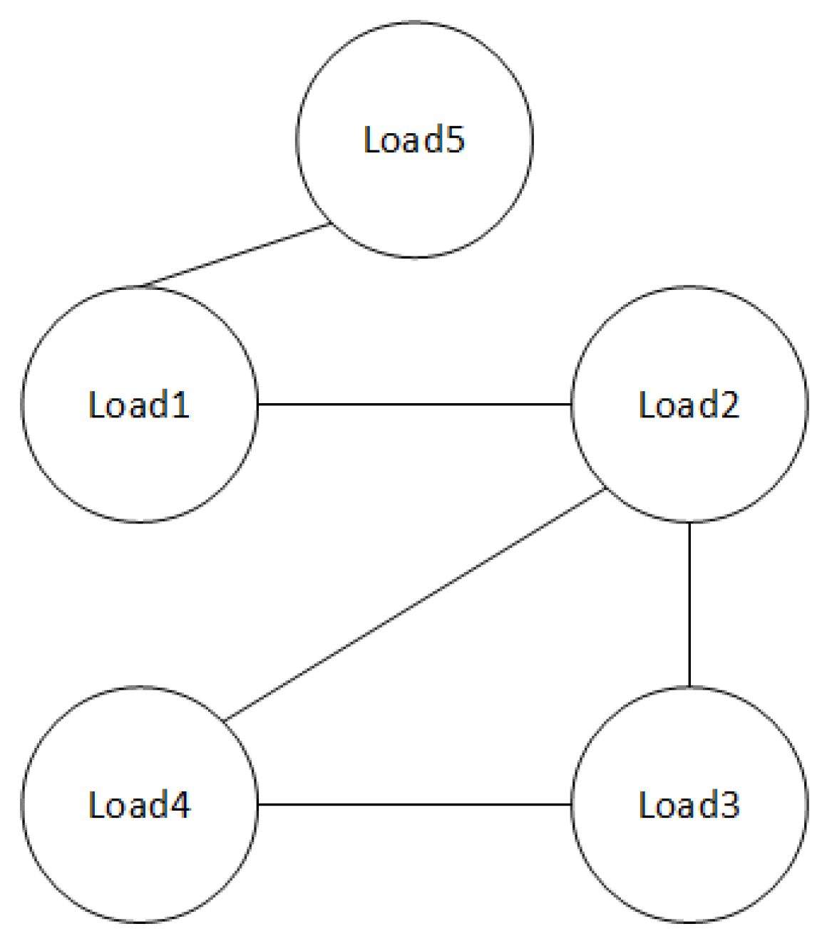
Since the information for each load needs to be centrally calculated for scheduling and allocation, the iterations from equations in (28) are centralized. However, in practical applications, centralized methods have many limitations. The entire system requires a centralized controller that connects all loads to calculate scheduling problems with wind power system model. Once this controller is attacked or damaged, the scheduling problems cannot be resolved adequately, leading to all loads not operating under normal conditions, which directly results in significant losses. Additionally, due to the presence of the centralized controller, the entire load topology is known and fixed in advance. Therefore, when a sudden event causes a load to disconnect, the overall system topology changes, and the controller cannot obtain global load information, preventing optimal scheduling of the overall system.

Using Equations (26) and (27), convert problem (23) into the following equivalent form:

$$\begin{array}{cc}\hfill & minF\left(p\right)=\sum _{i=1}^n{f}_i\left(p_i\right)\hfill \\ \hfill & \mathrm{subject}\mathrm{to}{\mathbf{1}}_n^{T}p=\Delta P_g\hfill \end{array}$$

(29)

Therefore, the gradient value of $F\left(p\right)$ can be expressed as:

$${\displaystyle \frac{\partial F_i\left(p_i\right)}{\partial p_i}}=\nabla f_i\left(p_i\right)+\rho \left(p_i-q_i^k+{\lambda }_i^k/\rho \right)$$

(30)

The cost of the controllable rotating device can be simulated as the following quadratic function:

$$C_i\left(P_i\right)=a_i{P}_i^2+b_i{P}_i+c_i$$

(31)

In the equation, $a_i,b_i$ and $c_i$ are the cost function coefficients related to load i, and $P_i$ is the power consumption of load i. Similarly, by setting $\overline{{\alpha }_i}=-b_i/\left(2a_i\right),\overline{{\beta }_i}=1/\left(2a_i\right)$ and ${\overline{\gamma }}_i=c_i-b_i^2/\left(4a_i\right)$, we can transform Equation (31) into another form:

$$C_i\left(P_i\right)={\displaystyle \frac{{\left(P_i-\overline{{\alpha }_i}\right)}^2}{2\overline{{\beta }_i}}}+\overline{{\gamma }_i}$$

(32)

There are also some positive and negative properties of the coefficients: $\overline{{\alpha }_i}\le 0,\overline{{\beta }_i}>0$ and ${\overline{\gamma }}_i\le 0$. The cost function i (31) and (32) are equivalent, and here the latter is used to simplify the subsequent analysis. Due to the similar structure of the supply-demand balance equality constraint in (23) and the controllable intelligent load and rotating equipment, the cost function of this type of load is often modeled in the same form as (31) and (32). Therefore, the negative benefits of the demand-side load can be obtained:

$$f_i\left(p_i\right)={\displaystyle \frac{{\left(p_i-{\alpha }_i\right)}^2}{2{\beta }_i}}+{\gamma }_i$$

(33)

In the equation, ${\alpha }_i,{\beta }_i$ and ${\gamma }_i$ have exactly the same properties as the aforementioned $\overline{{\alpha }_i},\overline{{\beta }_i}$ and $\overline{{\gamma }_i}$. Combining Equation (31) and the above equation, we can obtain:

$$\begin{array}{cc}\hfill {\varrho }_i& ={\displaystyle \frac{p_i-{\alpha }_i}{{\beta }_i}}+\rho \left(p_i-q_i^k+{\lambda }_i^k/\rho \right)\hfill \\ \hfill & ={\displaystyle \frac{\left(\rho {\beta }_i+1\right)p_i+{\beta }_i\left({\lambda }_i^k-\rho q_i^k\right)-{\alpha }_i}{{\beta }_i}}\hfill \end{array}$$

(34)

Since the power system network contains thousands of loads that belong to different users, using a distributed form inevitably involves exchanging information between neighboring users. Based on this consensus algorithm, the economic scheduling problem under supply and demand balance constraints can be quickly solved.

4. Experiments

4.1. Experimental Setup and Dataset of WPF

The proposed adaptive federated framework, which integrates AC and EWC for probabilistic WPF, was rigorously evaluated on the Global Energy Forecasting Competition 2014 ($\mathrm{GEFCom}2014$) WPF dataset. This dataset comprises historical records from seven distinct wind farms (${\mathrm{WF}}_0$ to ${\mathrm{WF}}_6$), each serving as an independent client in the FL (FL) framework, thus inherently possessing Non−IID data characteristics due to varying geographical and operational factors.

In the experiments on the GEFCom 2014 wind power dataset, we adopt a unified preprocessing pipeline for all wind farms. First, the raw time series are aligned to an hourly resolution, and any duplicated timestamps are removed by averaging the corresponding measurements. Missing values shorter than three consecutive hours are imputed by linear interpolation between the nearest available observations; for longer gaps, the entire day containing the gap is discarded from the dataset to avoid introducing large artificial jumps. To mitigate the influence of spurious spikes, we perform outlier detection using a three-sigma rule on a 24-h rolling window: any point whose deviation from the local mean exceeds three standard deviations is treated as an outlier and replaced by the local median within that window. The cleaned power series are then clipped to the interval $[0,{\mathrm{Cap}}_i]$, where ${\mathrm{Cap}}_i$ denotes the rated capacity of wind farm $W{F}_i$, to ensure physical plausibility. Finally, for each wind farm, all input features and target outputs are normalized to $[0,1]$ using min–max scaling computed on the training set only; the same scaling factors are applied to the validation and test sets. The resulting normalized sequences are then used to construct sliding windows of historical inputs and future prediction horizons for training the quantile regression model in the proposed FL framework.

Performance Comparison of Forecasting Methods

The predictive accuracy of the proposed methods is benchmarked against three essential baselines: Persistence, a simple time-series baseline; Local, a model trained exclusively on individual client data; and FL, the standard FL model (FedAvg). We introduce the $\mathrm{FL}+\mathrm{AR}$ (Adaptive Federated framework without EWC personalization) to isolate the benefit of the core federated and clustering strategy.

As evidenced by

Table 2. Comparison of Forecasting Errors Across Different Settings.

	Method	Forecasting Settings (WF)							Mean
		WF 0	WF 1	WF 2	WF 3	WF 4	WF 5	WF 6
24 h	Persistence	0.1003	0.1150	0.1246	0.1147	0.1249	0.1117	0.1147	0.1152
	Local	0.0805	0.0874	0.0934	0.0883	0.0899	0.0865	0.0885	0.0877
	FL	0.0742	0.0891	0.0918	0.0821	0.0876	0.0799	0.0857	0.0843
	FL + AR	0.0701	0.0850	0.0846	0.0799	0.0800	0.0756	0.0783	0.0796
12 h	Persistence	0.0804	0.0986	0.1030	0.0953	0.0987	0.0907	0.0975	0.0963
	Local	0.0819	0.0812	0.0858	0.0770	0.0762	0.0765	0.0931	0.0808
	FL	0.0688	0.0802	0.0835	0.0767	0.0791	0.0727	0.0787	0.0771
	FL + AR	0.0643	0.0640	0.0730	0.0708	0.0698	0.0680	0.0729	0.0691
4 h	Persistence	0.0533	0.0621	0.0691	0.0627	0.0641	0.0604	0.0643	0.0623
	Local	0.0476	0.0532	0.0580	0.0518	0.0538	0.0519	0.0544	0.0530
	FL	0.0474	0.0527	0.0581	0.0528	0.0533	0.0511	0.0542	0.0521
	FL + AR	0.0455	0.0524	0.0543	0.0488	0.0501	0.0507	0.0506	0.0503
2 h	Persistence	0.0427	0.0480	0.0552	0.0502	0.0512	0.0487	0.0516	0.0497
	Local	0.0348	0.0356	0.0413	0.0384	0.0375	0.0361	0.0374	0.0372
	FL	0.0338	0.0353	0.0406	0.0366	0.0369	0.0358	0.0374	0.0363
	FL + AR	0.0330	0.0347	0.0393	0.0357	0.0366	0.0347	0.0364	0.0361

, the following key observations can be drawn with respect to the forecast performance as follows. It is worth noting that Table 2 also reveals non-negligible variance in forecasting performance across different wind farms. In general, wind farms that exhibit more volatile and rapidly changing generation profiles tend to have slightly larger RMSE and MAE values than those with smoother wind patterns, regardless of the forecasting method. Nevertheless, the proposed FL + AC + EWC framework not only reduces the average error but also narrows the gap between the best- and worst-performing wind farms when compared with the persistence and purely local baselines. This suggests that sharing model parameters through federated learning helps less informative or more challenging sites benefit from data collected at other farms, thereby improving the overall uniformity and robustness of forecasting performance across the entire fleet.

To assess the quality of the full forecast distribution rather than only the median, we additionally compute the Continuous Ranked Probability Score (CRPS) for all methods. CRPS is defined as

$$\mathrm{CRPS}(F,y)={\int }_{-\infty }^{+\infty }{\left(F\left(z\right)-\mathbf{1}\{z\ge y\}\right)}^2\mathrm{d}z,$$

(35)

where F is the predictive cumulative distribution function and y is the realized outcome; lower values indicate better probabilistic calibration and sharpness.

Table 3. Average CRPS of different forecasting methods on GEFCom 2014.

Method	CRPS (Mean)
Persistence	0.072
Local LSTM	0.061
FedAvg (standard FL)	0.056
FL + AC	0.053
FL + AC + EWC (proposed)	0.049

summarizes the CRPS results averaged over all horizons and wind farms.

As shown in Table 3, the proposed FL + AC + EWC model achieves the lowest CRPS among all methods, indicating the best overall probabilistic performance. Compared with the persistence benchmark, CRPS is reduced by about 30%, and it improves upon purely local LSTM models and standard FedAvg by roughly 20% and 12%, respectively. FL + AC + EWC also yields around 7% lower CRPS than FL + AC without EWC, which confirms that EWC not only improves point metrics (RMSE/MAE) but also enhances the calibration and sharpness of the predictive distributions.

To further examine the calibration of the probabilistic forecasts, we evaluate the empirical coverage of central prediction intervals at different nominal levels. For each method and each interval $(1-2\alpha )$, we compute the fraction of realizations that fall inside the corresponding $(\alpha ,1-\alpha )$ quantile band and report the average coverage across all wind farms and horizons.

Table 4. Nominal vs empirical coverage (%) of central prediction intervals for different methods (averaged over all horizons and wind farms).

Method	50% Nominal	80% Nominal	90% Nominal
Persistence	44.1	73.2	83.5
Local LSTM	47.3	76.4	86.2
FedAvg (standard FL)	49.0	78.1	88.0
FL + AC	50.2	79.0	89.1
FL + AC + EWC (proposed)	51.0	81.2	90.4

compares the nominal and empirical coverage for 50%, 80%, and 90% intervals.

Table 4 shows that the proposed FL + AC + EWC method produces empirical coverages that are closest to the nominal levels across all three intervals, especially for high-coverage bands (80% and 90%). In contrast, the persistence and local LSTM baselines tend to be under-confident (empirical coverage noticeably below the nominal targets). This indicates that the proposed method not only lowers point forecast errors but also yields better calibrated prediction intervals, which is important for downstream dispatch and reserve allocation.

Figure 1 provides a visual summary of the mean RMSE results across all tested models and prediction horizons, directly correlating with the findings in Table 1. The primary trend observed is the consistent performance degradation as the forecasting lead time increases from $2\mathrm{h}$ to $24\mathrm{h}$, a universal challenge stemming from increasing uncertainty in long-term predictions. Crucially, the figure establishes a clear performance hierarchy: Persistence > Local > FL > $\mathrm{FL}+\mathrm{AR}$. The standard FL model consistently outperforms the Local approach, confirming the value of collaborative training across isolated data silos.

Figure 2 and Figure 3 provide a direct visual comparison of the probabilistic forecasting quality between the proposed $\mathrm{FL}+\mathrm{AC}+\mathrm{EWC}$ model and the Local model for the short-term $2\mathrm{h}$ horizon. The two key metrics assessed are Reliability (measured by PI coverage) and Sharpness (measured by PI width). While both models generally track the actual power output and its inherent volatility, the $\mathrm{FL}+\mathrm{AC}+\mathrm{EWC}$ framework demonstrates clear superiority. The proposed model’s PIs are visibly narrower across all confidence levels, particularly during periods of low generation, indicating superior Sharpness and providing a more informative forecast for grid operators.

Figure 4 and Figure 5 llustrate the probabilistic forecasting performance for the demanding $24\mathrm{h}$ horizon. Given the significantly longer lead time, the uncertainty inherently increases, as reflected by the generally wider Prediction Intervals (PIs) compared to the $2\mathrm{h}$ forecasts. Despite this challenge, the proposed $\mathrm{FL}+\mathrm{AC}+\mathrm{EWC}$ model (Figure 4) maintains a superior quality of forecast compared to the Local model. Notably, the Local model exhibits PIs that are substantially wider and more conservatively spread out, failing to provide the concise uncertainty quantification necessary for practical long-term planning.

Furthermore, the $\mathrm{FL}+\mathrm{AC}+\mathrm{EWC}$ model demonstrates better tracking of the actual peaks and troughs, especially on days with higher volatility (e.g., 8–9 June). The Local model, constrained by limited data and local non-IID challenges, appears to consistently under-predict or smooth out high-magnitude events, resulting in the actual value frequently touching or exceeding the upper bounds of the $80\%$ PI. This instability underscores the value of the EWC mechanism; by protecting global knowledge during local fine-tuning, the $\mathrm{FL}+\mathrm{AC}+\mathrm{EWC}$ model is more robust against local noise, allowing it to generate PIs that are both adequately reliable and maximally sharp, even in the highly uncertain long-term forecasting scenario.

To assess the effectiveness of the adaptive clustering and personalization mechanisms, we further conduct a clustering quality analysis and an EWC ablation study. For the latter, we construct two variants of the proposed framework: (i) FL + AC, which uses the Adaptive Clustering strategy but performs local fine-tuning without EWC, and (ii) FL + AC + EWC, which denotes the full proposed method with both AC and EWC enabled. For each wind farm, a local test set is held out, and we evaluate the two methods using RMSE, MAE, and the averaged Pinball Loss (averaged over all quantiles) on these local test sets. The results, averaged across the seven wind farms, are summarized in

Table 5. Effect of EWC on local personalization performance (GEFCom 2014, averaged over seven wind farms).

Method	RMSE	MAE	Pinball Loss
FL + AC	0.0578	0.0436	0.0312
FL + AC + EWC (proposed)	0.0549	0.0419	0.0298

.

As shown in Table 5, the FL + AC + EWC model consistently achieves lower RMSE, MAE, and averaged Pinball Loss than FL + AC on the local test sets, indicating that EWC effectively mitigates catastrophic forgetting during client-side personalization. By penalizing large deviations of important global parameters, EWC preserves shared knowledge while still allowing adaptation to local data, which yields more accurate probabilistic forecasts for each wind farm.

4.2. ADMM Dispatch

In this section, we validate the effectiveness of the aforementioned ADMM algorithm under two formulations—constrained and unconstrained—on the standard IEEE 14-bus and IEEE 30-bus test systems.

In the IEEE 14-bus and IEEE 30-bus simulations, the controllable loads are modeled with quadratic cost functions of the form

$$C_i\left(p_i\right)={\alpha }_i{p}_i^2+{\beta }_i{p}_i+{\gamma }_i,$$

where $p_i$ denotes the active power adjustment at bus i. The coefficients $({\alpha }_i,{\beta }_i,{\gamma }_i)$ are adapted from the standard quadratic generator cost data of the corresponding IEEE test systems. Specifically, we start from the quadratic cost coefficients provided in the widely used MATPOWER case files for the IEEE 14-bus and IEEE 30-bus systems and reinterpret them as the marginal cost profiles of controllable loads at the associated buses. To keep the numerical values consistent with the load-side formulation while preserving the relative cost structure, all coefficients are rescaled by a constant factor so that the resulting marginal costs fall in a typical range for distribution-level operation (approximately 10–50 monetary units per MWh). The values of $({\alpha }_i,{\beta }_i,{\gamma }_i)$ are kept fixed across all dispatch and anomaly detection scenarios. Due to the limitations on the number of load nodes and the rotational characteristics of intelligent loads, we can model some motors as intelligent load nodes for data transmission. In the IEEE-14 bus test system, there are three types of loads in total, and we provide the cost characteristic parameters of each load in

Table 6. Simulation parameters of the IEEE-14 bus test system.

⇄	DG1	DG2	DG3	DG4	DG5
$\alpha /MW$	−2535.2	−2535.2	−2023.2	−826.8	−2023.2
$\beta /MW$	352.1	352.1	257.7	103.7	257.7
$\gamma /MW$	−8616.8	−8616.8	−7631.0	−3216.7	−7631.0
Range/$MW$	[0, 500]	[0, 400]	[0, 300]	[0, 300]	[0, 400]

. The IEEE-14 bus test system includes five loads. It is assumed that the communication and actual lines in the entire system are independent of each other, and the specific communication topology can be referred to in Figure 6.

For convenience and simplification of analysis, in this system, load 1 and load 2 are set as the same type of load, load 3 and load 5 as the same type of load, while load 4 is a different type of load compared to the others. Due to the different lines and states of users, the scheduling range between intelligent loads of the same type is also different. At the same time, information transfer between loads is bidirectional. Thus, the adjacency matrix A of the topology in Figure 6 is obtained as

$$A=\left[\begin{array}{ccccc}1\hfill & 1\hfill & 0\hfill & 0\hfill & 1\hfill \\ 1\hfill & 1\hfill & 1\hfill & 1\hfill & 0\hfill \\ 0\hfill & 1\hfill & 1\hfill & 1\hfill & 0\hfill \\ 0\hfill & 1\hfill & 1\hfill & 1\hfill & 0\hfill \\ 1\hfill & 0\hfill & 0\hfill & 0\hfill & 1\hfill \end{array}\right]$$

(36)

Unless otherwise stated, all ADMM-based dispatch and anomaly detection experiments use a constant augmented Lagrangian penalty parameter $\rho =0.10$. The algorithm is terminated when both the primal and dual residual norms fall below a prescribed tolerance, i.e.,

$${\parallel r^k\parallel }_2\le ϵ,{\parallel s^k\parallel }_2\le ϵ,$$

with $ϵ={10}^{-4}$, or when a maximum number of iterations $K_{max}=200$ is reached. For anomaly detection, we define the detection threshold $\xi$ based on the steady-state residual statistics under normal operation: after the ADMM iterations have converged in the absence of anomalies, we compute the mean and standard deviation of the residual norm and set

$$\xi =\overline{r}+3{\sigma }_r\approx 0.02\mathrm{p}.\mathrm{u}.,$$

so that buses whose residual norms persistently exceed $\xi$ are flagged as abnormal with high confidence. These parameter settings are kept fixed for all scenarios on the IEEE 14-bus and IEEE 30-bus systems, ensuring that the reported results are fully reproducible.

To illustrate the impact of forecast uncertainty on dispatch, we consider two configurations: a “narrow-interval” setting that uses a lower quantile level $\underline{\alpha }=0.2$ (smaller $R\left(t\right)$) and a “wider-interval” setting with $\underline{\alpha }=0.1$ (larger $R\left(t\right)$). In the narrow-interval case, the required reserve margin is smaller, leading to a lower scheduled adjustment $\Delta P_g\left(t\right)$ but more frequent and larger corrective actions when realized wind power falls outside the too-tight prediction intervals. This manifests as slightly higher dispatch cost and a larger number of anomaly flags in the ADMM layer. In the wider-interval case, the reserve margin $R\left(t\right)$ is larger, so the scheduled adjustment is more conservative; although this increases the scheduled cost, the number and magnitude of corrective re-dispatch actions decrease, and the residual trajectories in ADMM are smoother. In our simulations, shifting from $\underline{\alpha }=0.2$ to $\underline{\alpha }=0.1$ increases the scheduled reserve by about 8% but reduces the number of large corrective adjustments by approximately 20%, illustrating the trade-off between upfront reserve allocation and ex-post corrective effort induced by forecast uncertainty.

To evaluate the anomaly detection capability of the proposed ADMM-based scheme in a realistic way, we construct three typical abnormal load behaviors that may occur in industrial distribution networks.

Scenario S1 (20% sudden surge): at a selected load bus, the active power demand experiences an instantaneous increase to $1.2$ times its nominal value and remains at this elevated level for at least 10 consecutive dispatch intervals, emulating a sudden connection of additional production equipment.

Scenario S2 (50% sudden drop): at a selected load bus, the active power demand suddenly decreases to $0.5$ times its nominal value, representing an abrupt shutdown of a large industrial process.

Scenario S3 (sustained 15% deviation): at a selected load bus, the active power demand is gradually ramped to $1.15$ times its nominal value over a few intervals and then remains at this level for the rest of the simulation horizon, mimicking a slowly evolving but persistent change in consumption.

In all cases, anomalies are injected after the ADMM iterations have converged to a steady operational point, so that the subsequent deviations in local residuals and multipliers are solely attributable to the abnormal behaviors.

For each scenario, the anomaly detection performance is evaluated using the following metrics. A detection is counted as a true positive (TP) if an anomalous bus is correctly flagged within a finite number of ADMM iterations after the anomaly is injected; a false negative (FN) occurs when an anomalous bus is never flagged. A false positive (FP) is recorded when a normal bus is incorrectly flagged as abnormal. The accuracy is defined as the ratio of correctly classified buses (both normal and abnormal) to the total number of buses. The false positive rate (FPR) is the proportion of normal buses that are incorrectly flagged, and the false negative rate (FNR) is the proportion of anomalous buses that remain undetected. The average detection delay (ADE) is measured as the number of ADMM iterations between the time when the anomaly is injected and the first iteration at which the corresponding bus is flagged as abnormal.

Table 7. Anomaly detection performance of the ADMM-based scheme under different abnormal load scenarios.

Scenario	Accuracy (%)	FPR (%)	FNR (%)	ADE (Iterations)
S1: 20% sudden surge	97.8	2.3	2.1	3.2
S2: 50% sudden drop	96.5	3.4	3.7	3.8
S3: sustained 15% deviation	95.1	4.1	4.8	4.6
Overall average	96.5	3.3	3.5	3.9

summarizes these metrics averaged over multiple realizations of each scenario on the IEEE 14-bus and IEEE 30-bus systems.

Because the algorithm can be given any initial value, but must satisfy the equality constraint of supply-demand balance, a total scheduling deviation of 1500 MW is given. The load power deviations at the initial moment are as follows: $p_1\left(0\right)=490.0\mathrm{MW}$, $p_2\left(0\right)=410.0\mathrm{MW}$, $p_3\left(0\right)=300.0\mathrm{MW}$, $p_4\left(0\right)=150.0\mathrm{MW}$, $p_5\left(0\right)=150.0\mathrm{MW}$. The positive scalar gain value is given as a constant. Using the above data and the topology, the optimal scheduling problem without inequality constraints can be easily calculated in advance, and the optimal solution is: $p_1^{*}=509.7\mathrm{MW}$, $p_2^{*}=509.7\mathrm{MW}$, $p_3^{*}=205.3\mathrm{MW}$, $p_4^{*}=70.0\mathrm{MW}$, $p_5^{*}=205.2\mathrm{MW}$.

As shown in Figure 7, without being constrained by anomaly thresholds [38], the proposed algorithm can effectively detect load power deviations during periods of abnormal power consumption within the industry chain, and its detection time is significantly improved compared to the consensus algorithm in the literature. Similarly, when performing distributed sub-problem anomaly detection, the anomaly evaluation metrics for each sub-problem are also consistent, as shown in Figure 8.

As shown in Figure 9, the consistency balance of anomaly identification is always maintained during the detection process to ensure that the equality constraint is satisfied. This is a necessary guarantee for the accuracy of the upstream and downstream industrial power anomaly monitoring system. Figure 10 respectively shows the anomaly detection scheme with upper and lower limit constraints of power consumption characteristics.

Figure 7, Figure 8, Figure 9 and Figure 10 compare the trajectories of the dispatch variables and residuals in the unconstrained and constrained cases. In the unconstrained setup, all buses can freely share the required adjustment, and the ADMM iterations converge smoothly to a solution where the incremental costs are equalized across the network. Once the box constraints $p_i^{min}\le p_i\le p_i^{max}$ are enforced, several buses quickly reach their individual limits and remain saturated. Physically, this means that these loads have exhausted their flexibility and can no longer contribute to compensating the wind power deviation. Consequently, the remaining imbalance must be reallocated to the unsaturated buses, leading to the kinked trajectories and slightly slower decrease of the primal and dual residuals observed in the constrained case. Despite this effect, the algorithm still converges in a reasonable number of iterations because the overall problem remains convex and the active-set of constrained loads stabilizes after a few iterations. The constrained solution is therefore more realistic from an operational viewpoint, as it respects individual load capabilities, while the unconstrained solution mainly serves as a reference for the best achievable economic performance in the absence of physical limits.

5. Discussion

The ADMM-based load-side dispatch and anomaly detection scheme in Section 3.2 takes as input the probabilistic wind power forecasts generated by the adaptive FL framework described in Section 3.1. In particular, the scheduled wind power trajectory is derived from a central quantile (e.g., the median) of the forecast distribution, while a safety margin based on the lower quantiles is incorporated into the reserve allocation. When the forecasts are accurate and well calibrated, the realized wind generation remains within the predicted intervals with high probability, and only small adjustments of controllable loads are needed to maintain power balance. Consequently, the ADMM iterations converge quickly with small residuals, the overall dispatch cost is reduced, and only a few anomaly flags are raised. In contrast, systematic forecast bias or overly narrow prediction intervals increase the probability of large imbalances between scheduled and actual wind power, which leads to more frequent and larger corrective actions, slower convergence of the distributed optimization, and a higher rate of anomaly alarms. The improvements in RMSE, MAE, and Pinball Loss achieved by the proposed FL-based probabilistic forecasting thus translate into fewer re-dispatch operations and more stable ADMM trajectories in our simulations, highlighting the practical value of better forecasting quality for the downstream optimization and anomaly detection tasks.

To further assess the practical deployability of the proposed framework, we quantitatively evaluate its communication and computation overhead using the implementation adopted in our experiments. For the FL-based probabilistic wind power forecasting, the artificial neural network deployed at each client contains approximately $5.3\times {10}^4$ trainable parameters. With 32-bit floating-point representation, this corresponds to about $0.21$ MB of model data. In each global FL round, every wind farm uploads its local model parameters to the server (or cluster center) and receives the aggregated global (or cluster-specific) parameters once, leading to a per-client communication volume of roughly $0.42$ MB per round (upload + download) and a total volume of about $2.9$ MB per round when seven wind farms participate. Over 100 global rounds, the overall communication volume remains below 300 MB, which is well within the capacity of typical industrial communication infrastructures.

On the computation side, all experiments are run on a workstation equipped with an Intel Core i7 CPU (8 cores, 2.5 GHz) and 16 GB RAM without GPU acceleration. Under this setup, the average client-side latency for one FL round (including one local training epoch and communication) is approximately $0.38$ s. For the ADMM-based load-side dispatch and anomaly detection, the per-iteration computational complexity at node i is linear in both the number of incident edges and the dimension of local decision variables, i.e., $\mathcal{O}\left(\right|{\mathcal{N}}_i\left|d\right)$, where $|{\mathcal{N}}_i|$ denotes the number of neighbors of node i and d denotes the number of local variables. In practice, this results in an average wall-clock time of about 5 ms per iteration for the IEEE 14-bus system and about 8 ms per iteration for the IEEE 30-bus system. Since the ADMM algorithm typically converges within a few tens of iterations, the total latency for one distributed dispatch and anomaly detection cycle is on the order of a few hundred milliseconds, which is compatible with standard dispatch intervals in distribution-level operation.

As summarized in

Table 8. Communication and computation overhead of the proposed framework.

Component/Metric	Symbol	Value	Description
FL model size (per client)	$\left|\theta \right|$	≈$5.3\times {10}^4$ params	Number of trainable ANN parameters
FL comm. per client per round	$V_{\mathrm{FL}}^{\left(\mathrm{cli}\right)}$	≈$0.42$ MB	Upload + download model parameters
FL comm. per round (7 clients)	$V_{\mathrm{FL}}^{\left(\mathrm{tot}\right)}$	≈$2.9$ MB	Total across all wind farms
Client-side FL latency per round	$T_{\mathrm{FL}}$	≈$0.38$ s	One local epoch + communication
ADMM per-iteration complexity	$C_{\mathrm{ADMM}}$	$\mathcal{O}\left(\right|{\mathcal{N}}_i\left|d\right)$	Node i: neighbors $|{\mathcal{N}}_i|$, dim. d
ADMM iteration latency (14-bus)	$T_{\mathrm{ADMM}}^{14}$	≈5 ms	Average per iteration per node
ADMM iteration latency (30-bus)	$T_{\mathrm{ADMM}}^{30}$	≈8 ms	Average per iteration per node

, the communication volume per FL round is on the order of a few megabytes even when all seven wind farms participate, and the client-side computation latency per FL round is below one second on a standard CPU-only workstation. The ADMM-based dispatch and anomaly detection scheme exhibits linear per-iteration complexity in the local neighborhood size and achieves millisecond-level iteration latency for both the IEEE 14-bus and IEEE 30-bus systems. These results indicate that the end-to-end framework is computationally efficient and communication-feasible for deployment in practical industrial power networks with similar scales.

While the proposed adaptive FL-based probabilistic forecasting framework with AC and EWC has shown promising results on the GEFCom 2014 wind farms and IEEE test systems, several limitations remain. First, although our overhead evaluation indicates that the communication and computation costs are moderate for the considered setup (a small number of wind farms and a medium-size ANN), the total communication volume of FL still grows roughly linearly with both the number of participating clients and the number of global rounds. In large-scale deployments with tens or hundreds of wind farms and more complex models, this could lead to non-negligible communication burden, especially over bandwidth-limited or latency-sensitive industrial networks. Techniques such as model compression, sparsified or quantized updates, and probabilistic client subsampling are promising directions to further reduce communication without significantly degrading forecasting accuracy. Second, the current FL scheme assumes that a central server (or a small number of cluster centers) can reliably coordinate communication rounds in a mostly synchronous manner. In practice, connectivity may be intermittent and client availability may be highly variable, which calls for more scalable and robust variants such as hierarchical or fully decentralized federated learning with asynchronous updates. Third, although the adaptive clustering and EWC components help mitigate the impact of Non-IID data and catastrophic forgetting, they do not explicitly account for long-term concept drift (e.g., structural changes in wind regimes or operating patterns). Extending the framework with drift detection mechanisms and dynamically adaptable model architectures is an important topic for future work. Despite these limitations, the present results demonstrate the feasibility of combining federated probabilistic forecasting with distributed optimization for industrial grids, and they provide a basis on which more scalable and communication-efficient designs can be developed.

6. Conclusions

This paper proposed an integrated framework that combines federated probabilistic wind power forecasting with ADMM-based load-side dispatch and distributed anomaly detection for privacy-constrained industrial power networks. An adaptive FL scheme with AC and EWC was used to train quantile regression models across multiple wind farms without sharing raw data, and the resulting forecasts were embedded into a distributed ADMM formulation that coordinates controllable loads and localizes abnormal behaviours. Experiments on the GEFCom 2014 dataset and IEEE 14-bus/30-bus systems show that the proposed FL + AC + EWC forecaster reduces RMSE and MAE by up to about 20% and 18% compared with persistence, achieves 8–15% improvements over purely local models, and provides an additional 3–5% gain over FL + AC without EWC. The downstream ADMM-based scheme converges in a few tens of iterations and attains anomaly detection accuracy above 95% with low false-alarm rates, while incurring moderate communication and computation overhead. These results indicate that improving probabilistic forecasting via adaptive federated learning can directly enhance the efficiency and robustness of distributed dispatch and anomaly detection in decentralized power systems.