Statistical Inference for Two Lomax Populations Under Balanced Joint Progressive Type-II Censoring Scheme

Abstract

In recent years, joint censoring schemes have gained significant attention in lifetime experiments and reliability analysis. A refined approach, known as the balanced joint progressive censoring scheme, has been introduced in statistical studies. This research focuses on statistical inference for two Lomax populations under this censoring framework. Maximum likelihood estimation is employed to derive parameter estimates, and asymptotic confidence intervals are constructed using the observed Fisher information matrix. From a Bayesian standpoint, posterior estimates of the unknown parameters are obtained under informative prior assumptions. To evaluate the effectiveness and precision of these estimators, a numerical study is conducted. Additionally, a real dataset is analyzed to demonstrate the practical application of these estimation methods.

1. Introduction

With the increasing reliability of modern products, censored data have become essential in survival analysis, reliability assessments, and medical research. They play a crucial role in minimizing both the time and cost of life-testing experiments. Depending on the study’s objectives, different censoring strategies can be employed, with Type-I and Type-II censoring being the most widely used.

However, neither of these schemes permits the removal of experimental units during life testing. To address this limitation, the progressive censoring scheme introduces flexibility by allowing units to be withdrawn throughout the experiment. In particular, the progressive Type-II censoring scheme enables unit removal while ensuring that a predetermined number of failures are recorded, thereby improving the efficiency of the experiment. Kyeongjun and Youngseuk [1] explored both classical and Bayesian approaches to estimate parameters, hazard functions, and reliability functions of the inverted exponentiated half-logistic distribution within a progressive Type-II censoring scheme. Gürünlü Alma and Arabi Belaghi [2] focused on the complementary exponential geometric distribution under the same censoring framework, employing the Structural Equation Modeling algorithm alongside the Markov Chain Monte Carlo (MCMC) method for parameter estimation. The inference of the inverted exponentiated Rayleigh distribution using an adaptive Type-II progressive hybrid censored sample, along with Bayesian estimation via the MCMC method and the Metropolis–Hastings (M-H) algorithm, was presented in Panahi and Moradi’s study [3]. Panahi and Asadi’s work [4] featured parameter estimation for the Burr Type-III distribution under the same censoring model, where Bayesian estimates were derived through the Lindley method and the M-H sampling technique.

Previous studies have primarily focused on analyzing a single population, with relatively little attention given to research involving multiple samples. However, in recent years, two-sample joint censoring schemes have gained increasing attention due to their ability to effectively reduce time and costs in life-testing experiments. Under the Type-II joint censoring scheme, two independent samples are tested simultaneously until a predetermined number of failures occur. This approach allows for more efficient data collection on the lifetimes of different samples, enabling more comprehensive comparisons and analyses under the same experimental conditions. Not only does this method improve data utilization efficiency, but it also enhances the practical applicability of experiments, making it widely valuable in fields such as reliability analysis and product quality assessment. Balakrishnan and Rasouli [5] proposed a Type-II censoring scheme for two populations and developed a parameter estimation method for two exponential distributions. Ashour and Abo-Kasem [6] applied this approach to conduct classical inference for two Weibull populations. Expanding on this, Mondal and Kundu [7] extended the framework to generalized exponential distributions with two parameters, employing both maximum likelihood and Bayesian estimation. Furthermore, the issue of interval estimation for two Weibull populations under a joint Type-II progressive censoring scheme was addressed in Parsi and Ganjali’s study [8]. Balakrishnan [9] established the conditional maximum likelihood estimates and Bayesian estimates for the k exponential mean parameters, utilizing a joint progressively Type-II censored sample from k independent exponential populations. Similarly, statistical inference for the three-parameter Burr-XII distribution under a joint progressive Type-II censoring scheme for two independent samples was explored in Mohamed and Mustafa’s paper [10], where both maximum likelihood and Bayesian estimation methods were applied. Ismail [11] introduces an adaptive Type-I progressively hybrid censoring scheme under a step-stress partially accelerated test model, offering advantages over existing schemes.

More recently, Mondal and Kundu [12] introduced the balanced joint progressive Type-II censoring (B-JPC) scheme, considering it superior to the conventional JPC method. In contrast to the traditional approach, the B-JPC scheme is more practical and easier to implement. Moreover, estimators derived from this scheme are not only simpler to compute but also demonstrate better performance compared to those obtained using the JPC method. It has drawn much attention in comparative lifetime testing in reliability engineering. As pointed out by Mondal and Kundu [13], Bayesian inference for two Weibull populations sharing a common shape parameter but with different scale parameters was examined under the B-JPC scheme. Statistical inference for two Lindley populations, along with criteria for optimal censoring design, was presented in Goel and Krishna’s study [14]. Similarly, Shi and Gui’s paper [15] addressed parameter estimation for two Gompertz populations.

The Lomax distribution (LD), introduced by Lomax [16], also known as the Pareto II distribution, was initially designed to model business failures. However, its applications extend far beyond this original use. Over the years, it has proven to be a useful tool in various fields, particularly reliability modeling and life testing, as emphasized by Hassan and Al-Ghamdi [17]. The LD has become widely adopted to analyze diverse datasets. Moreover, as highlighted by Holland [18], the LD is applicable across a wide range of fields, including biological sciences and the distribution of computer file sizes on servers. Mahmoud [19] proposed a lifetime performance index based on progressive Type-II sampling under the Lomax distribution and evaluated the performance of the maximum likelihood and Bayesian methods in estimating the lifetime performance index. Pak and Mahmoudi [20] applied the Newton–Raphson method and the EM algorithm to obtain the maximum likelihood estimates of the Lomax distribution parameters under the progressive Type-II censoring scheme. Furthermore, Bayesian estimates were computed and compared using Monte Carlo simulations in terms of estimation bias and mean squared error. Mustafa [21] performed Bayesian inference for two Lomax populations under joint progressive Type-II censoring, with an emphasis on engineering applications.

This paper addresses the estimation challenges related to the LD. We derive maximum likelihood estimators (MLEs) for the unknown parameters; however, we find that the MLEs cannot be expressed in closed form. To resolve this, we propose approximate maximum likelihood estimators (AMLEs) that can be explicitly calculated. We also employ the asymptotic distribution of the MLEs and the bootstrap method to construct confidence intervals (CIs) for the unknown parameters. In addition, we perform Bayesian inference, assuming independent Gamma priors, and compute Bayesian estimators under squared error (SE) and linear exponential (LINEX) loss functions. To assess the performance of these estimators, we conduct Monte Carlo simulations and compare point estimates based on their mean values and mean squared error (MSE). Furthermore, we evaluate the effectiveness of 95% two-sided interval estimates by analyzing their average confidence lengths, ensuring a comprehensive assessment of interval estimation precision. To further validate our methodology, we conduct a comparative analysis between frequentist and Bayesian approaches, highlighting their respective advantages and limitations in different parameter settings. Lastly, we apply our methodology to real data to demonstrate its practical application and effectiveness, illustrating its potential use in real statistical inference problems.

The structure of this paper is as follows: Section 2 outlines the B-JPC scheme and formulates the model. The maximum likelihood estimation and the coverage probabilities of the model parameters are discussed, deriving asymptotic confidence intervals using the observed Fisher information matrix (FIM) in Section 3. Section 4 presents Bayesian estimation methods, employing the Metropolis–Hastings algorithm. Section 5 provides numerical simulations and real data analysis. Lastly, Section 6 summarizes the findings and concludes this study.

2. Model Description

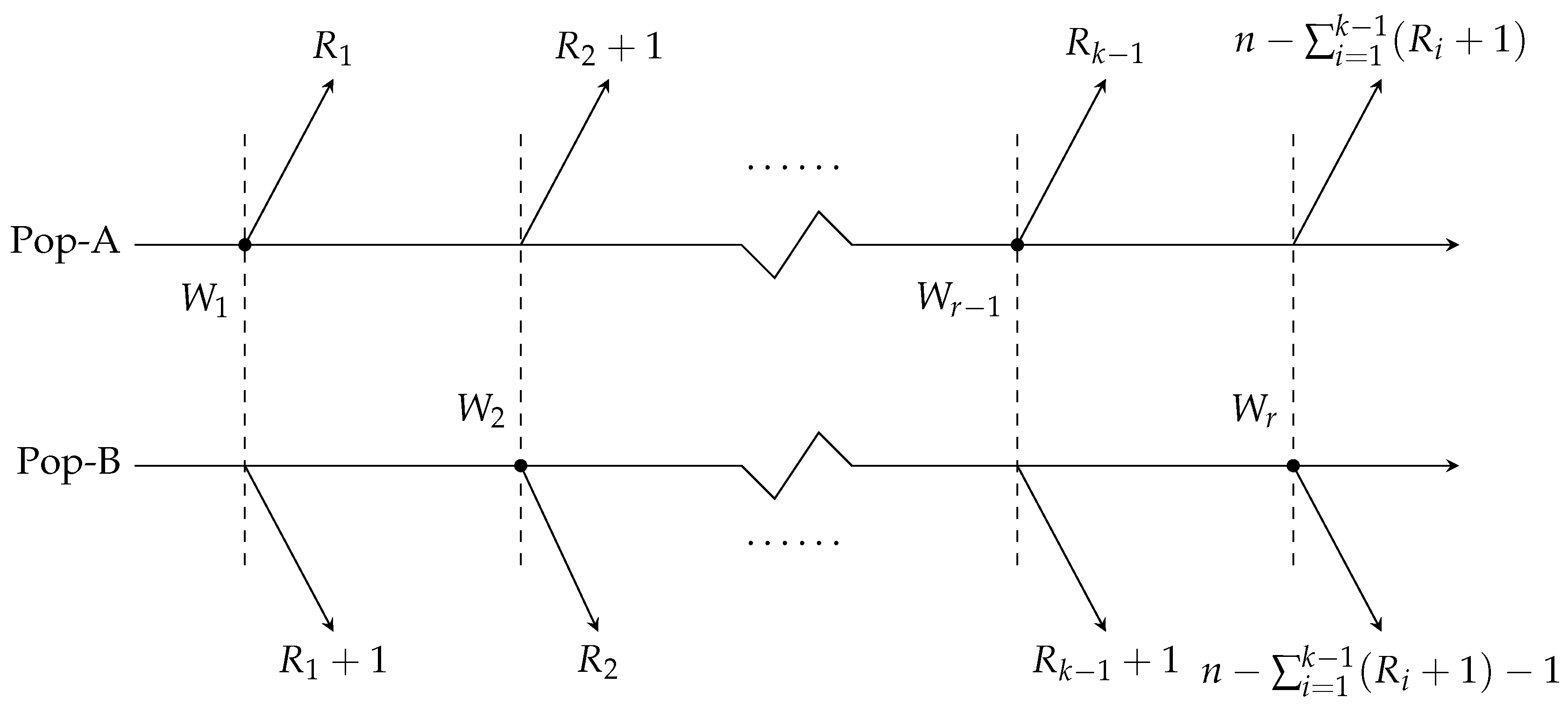
The B-JPC scheme is described as follows. Consider two similar products, denoted as A and B, for which we need to compare their relative performance. We draw a sample of size n from each product population, known as Pop-A and Pop-B. Let k denote the total number of failures observed in the life-testing experiment, where $k<n$. The removal pattern R, given by $R_1, R_2,\dots ,R_k$, consists of non-negative integers such that ${\sum }_{i=1}^{k-1}(R_i+1)<n$, and each $R_i\ge 0$.

In the B-JPC scheme, both populations undergo testing simultaneously. When the first failure occurs in Pop-A at time $W_1$, $R_1$ units are randomly removed from its remaining $n-1$ surviving units, while $R_1+1$ units are removed from the n surviving units of Pop-B. If the second failure occurs in Pop-B at time $W_2$, then $R_2+1$ units are withdrawn from the remaining $n-R_1-1$ units of Pop-A, and $R_2$ units are removed from the remaining $n-R_1-2$ units of Pop-B. This process continues, with each subsequent failure triggering the removal of units from either Pop-A or Pop-B, until a total of k failures are observed, at which point the experiment concludes.

This life-testing experiment introduces a new set of random variables, Z.

$$Z_i=\left\{\begin{array}{c}1,W_i\in \mathrm{Pop}-A\hfill \\ 0,\mathrm{otherwise}\hfill \end{array}\right.$$

Let $k_1$ and $k_2$ denote the number of failures from Pop-A and Pop-B, respectively. The random variables $Z_i$ indicate whether the i-th failure is from Pop-A ($Z_i=1$) or Pop-B ($Z_i=0$). The total number of failures from Pop-A and Pop-B is $k_1={\sum }_{i=1}^k{Z}_i$ and $k_2=k-k_1$, respectively. A schematic of the B-JPC scheme is provided in Figure 1.

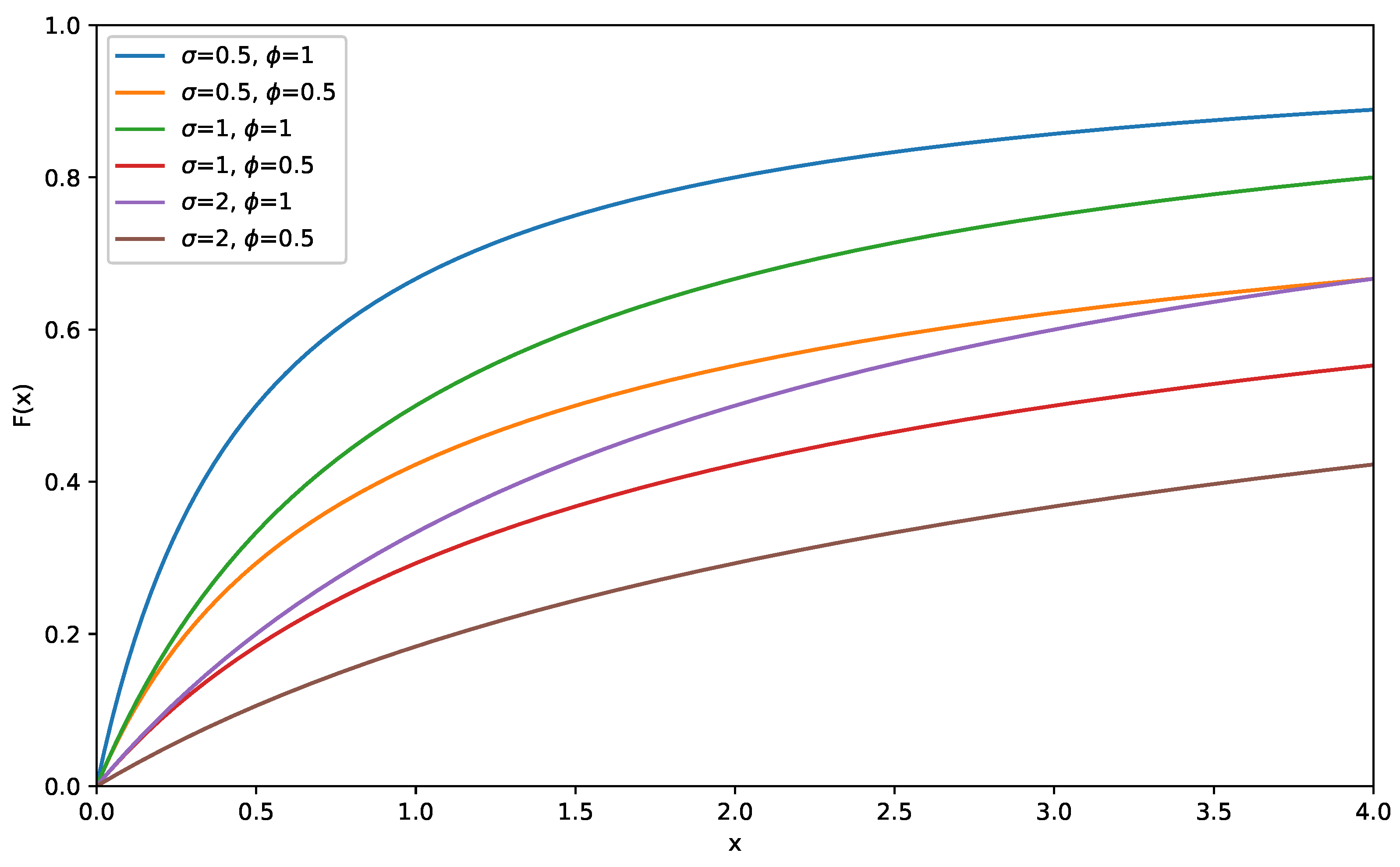
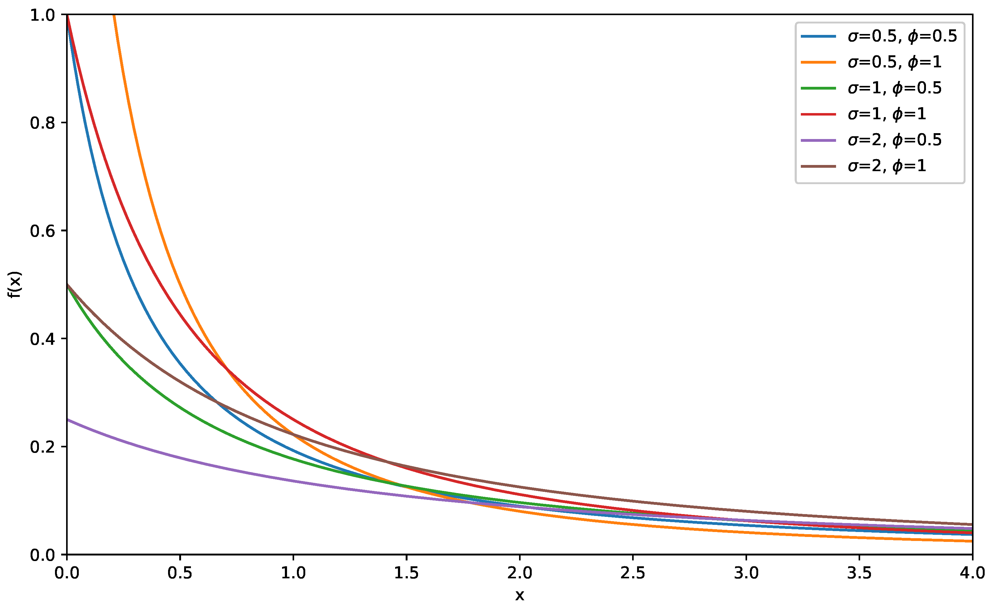
Suppose that the random variable W follows the Lomax distribution, denoted as $W\sim LD(\sigma ,\varphi )$. The cumulative distribution function (CDF) is defined as follows:

$$F\left(x\right)=1-{\left(1+{\displaystyle \frac{x}{\sigma }}\right)}^{-\varphi },x>0,\sigma ,\varphi >0.$$

(1)

Moreover, its corresponding probability density function (PDF) is expressed as follows:

$$f\left(x\right)={\displaystyle \frac{\varphi }{\sigma }}{\left(1+{\displaystyle \frac{x}{\sigma }}\right)}^{-\varphi -1},x>0,\sigma ,\varphi >0.$$

(2)

In these functions, $\sigma$ represents the scale parameter, while $\varphi$ denotes the shape parameter. Figure 2 and Figure 3 present graphs illustrating the CDF and PDF of the LD for various values of $\varphi$ and $\sigma$.

We assume that the lifetimes of the n units from product Pop-A, denoted as $X_1,\dots ,X_n$, are independent and identically distributed (i.i.d.) random variables that follow the Lomax distribution, LD$({\sigma }_1,{\varphi }_1)$. Similarly, the lifetimes of the n units from product Pop-B, denoted as $Y_1,\dots ,Y_n$, are i.i.d. random variables following the Lomax distribution, LD$({\sigma }_2,{\varphi }_2)$. For a given B-JPC scheme R, the observed sample data are expressed as $\mathrm{data}=((W_1,Z_1),\dots ,(W_k,Z_k))$, where $W_i$ represents the failure time at the i-th instance. The indicator $Z_i$ denotes the population from which the failure originates: $Z_i=1$ corresponds to a failure occurring in Pop-A, while $Z_i=0$ indicates a failure in Pop-B. The total number of failures in Pop-A is given by $k_1={\sum }_{i=1}^k{Z}_i$, whereas the number of failures in Pop-B is $k_2={\sum }_{i=1}^k(1-Z_i)=k-k_1$.

3. Classical Estimation

3.1. Maximum Likelihood Estimators

Based on the censoring mechanism described above, the contribution of $(W_i,Z_i=1,R_i)$ to the likelihood is

$$P(W_i,Z_i=1,R_i)={\left({\displaystyle \frac{{\varphi }_1}{{\sigma }_1}}{\left(1+{\displaystyle \frac{W_i}{{\sigma }_1}}\right)}^{-{\varphi }_1-1}\right)}^{Z_i}\times {\left({\left(1+{\displaystyle \frac{W_i}{{\sigma }_1}}\right)}^{-{\varphi }_1}\right)}^{R_i}\times {\left({\left(1+{\displaystyle \frac{W_i}{{\sigma }_2}}\right)}^{-{\varphi }_2}\right)}^{R_i+1}.$$

The contribution of $(W_i,Z_i=0,R_i)$ to the likelihood is given by

$$P(W_i,Z_i=0,R_i)={\left({\displaystyle \frac{{\varphi }_2}{{\sigma }_2}}{\left(1+{\displaystyle \frac{W_i}{{\sigma }_2}}\right)}^{-{\varphi }_2-1}\right)}^{1-Z_i}\times {\left({\left(1+{\displaystyle \frac{W_i}{{\sigma }_1}}\right)}^{-{\varphi }_1}\right)}^{R_i+1}\times {\left({\left(1+{\displaystyle \frac{W_i}{{\sigma }_2}}\right)}^{-{\varphi }_2}\right)}^{R_i}.$$

Hence, the contribution of a general $(W_i,Z_i,R_i)$ can be written as

$$P(W_i,Z_i,R_i)={({\displaystyle \frac{{\varphi }_1}{{\sigma }_1}})}^{Z_i}{({\displaystyle \frac{{\varphi }_2}{{\sigma }_2}})}^{1-Z_i}\times {\left(1+{\displaystyle \frac{W_i}{{\sigma }_1}}\right)}^{Z_i(-{\varphi }_1-1)-{\varphi }_1(R_i+1-Z_i)}\times {\left(1+{\displaystyle \frac{W_i}{{\sigma }_2}}\right)}^{(1-Z_i)(-{\varphi }_2-1)-{\varphi }_2(R_i+Z_i)}.$$

Therefore, the likelihood function of the unknown parameters $\left({\sigma }_1,{\sigma }_2,{\varphi }_1,{\varphi }_2\right)$ based on the removal pattern R and the observed data is given by

$$L({\sigma }_1,{\sigma }_2,{\varphi }_1,{\varphi }_2|data)=C{({\displaystyle \frac{{\varphi }_1}{{\sigma }_1}})}^{k_1}\times {({\displaystyle \frac{{\varphi }_2}{{\sigma }_2}})}^{k_2}\times \prod _{i=1}^k{\left(1+{\displaystyle \frac{W_i}{{\sigma }_1}}\right)}^{-{\varphi }_1{R}_i-{\varphi }_1-Z_i}\times \prod _{i=1}^k{\left(1+{\displaystyle \frac{W_i}{{\sigma }_2}}\right)}^{-{\varphi }_2{R}_i-{\varphi }_2+Z_i-1},$$

(3)

$$C=\prod _{i=1}^k\left(n-\sum _{j=1}^{i-1}(R_j+1)\right),$$

$$k_1=\sum _{i=1}^k{Z}_i,k_2=\sum _{i=1}^k(1-Z_i)=k-k_1.$$

The log-likelihood function corresponding to (3) can be expressed as follows:

$$lnL=lnC+k_{1}ln{\displaystyle \frac{{\varphi }_1}{{\sigma }_1}}+k_{2}ln{\displaystyle \frac{{\varphi }_2}{{\sigma }_2}}+\sum _{i=1}^k(-{\varphi }_1{R}_i-{\varphi }_1-Z_i)ln(1+{\displaystyle \frac{W_i}{{\sigma }_1}})+\sum _{i=1}^k(-{\varphi }_2{R}_i-{\varphi }_2+Z_i-1)ln(1+{\displaystyle \frac{W_i}{{\sigma }_2}}).$$

(4)

Therefore, the normal equations are derived by computing the partial derivatives of the log-likelihood function (4) and equating them to zero, as demonstrated below.

$${\displaystyle \frac{\partial lnL}{\partial {\sigma }_1}}=-{\displaystyle \frac{k_1}{{\sigma }_1}}+\sum _{i=1}^k{\displaystyle \frac{({\varphi }_1{R}_i+{\varphi }_1+Z_i)\frac{W_i}{{{\sigma }_1}^2}}{1+\frac{W_i}{{\sigma }_1}}}=0,$$

(5)

$${\displaystyle \frac{\partial lnL}{\partial {\sigma }_2}}=-{\displaystyle \frac{k_2}{{\sigma }_2}}+\sum _{i=1}^k{\displaystyle \frac{({\varphi }_2{R}_i+{\varphi }_2+1-Z_i)\frac{W_i}{{{\sigma }_2}^2}}{1+\frac{W_i}{{\sigma }_2}}}=0,$$

(6)

$${\displaystyle \frac{\partial lnL}{\partial {\varphi }_1}}={\displaystyle \frac{k_1}{{\varphi }_1}}+\sum _{i=1}^k(-R_i-1)ln(1+{\displaystyle \frac{W_i}{{\sigma }_1}})=0,$$

(7)

$${\displaystyle \frac{\partial lnL}{\partial {\varphi }_2}}={\displaystyle \frac{k_2}{{\varphi }_2}}+\sum _{i=1}^k(-R_i-1)ln(1+{\displaystyle \frac{W_i}{{\sigma }_2}})=0.$$

(8)

To obtain the MLEs of ${\sigma }_1$, ${\sigma }_2$, ${\varphi }_1$, and ${\varphi }_2$, we need to solve Equations (5) to (8) simultaneously. However, due to their complexity, deriving closed-form solutions for each parameter is not practical. Hence, numerical approaches like the Newton–Raphson method are commonly employed for parameter estimation.

3.2. Approximate Confidence Interval

The second-order partial derivatives of the log-likelihood function (4) with respect to ${\sigma }_1$, ${\sigma }_2$, ${\varphi }_1$, and ${\varphi }_2$ result in

$${\displaystyle \frac{{\partial }^{2}lnL}{\partial {\sigma }_1^2}}={\displaystyle \frac{k_1}{{\sigma }_1^2}}+\sum _{i=1}^k{\displaystyle \frac{W_i(W_i+2{\sigma }_1)({\varphi }_1{R}_i+{\varphi }_1+Z_i)}{{({\sigma }_1^2+{\sigma }_1{W}_i)}^2}},$$

$${\displaystyle \frac{{\partial }^{2}lnL}{\partial {\sigma }_2^2}}={\displaystyle \frac{k_2}{{\sigma }_2^2}}+\sum _{i=1}^k{\displaystyle \frac{W_i(W_i+2{\sigma }_2)({\varphi }_2{R}_i+{\varphi }_2+1-Z_i)}{{({\sigma }_2^2+{\sigma }_2{W}_i)}^2}},$$

$${\displaystyle \frac{{\partial }^{2}lnL}{\partial {\varphi }_1^2}}=-{\displaystyle \frac{k_1}{{\varphi }_1^2}},$$

$${\displaystyle \frac{{\partial }^{2}lnL}{\partial {\varphi }_2^2}}=-{\displaystyle \frac{k_2}{{\varphi }_2^2}},$$

$${\displaystyle \frac{{\partial }^{2}lnL}{\partial {\sigma }_1\partial {\varphi }_1}}={\displaystyle \frac{{\partial }^{2}lnL}{\partial {\varphi }_1\partial {\sigma }_1}}=\sum _{i=1}^k{\displaystyle \frac{(R_i+1)\frac{W_i}{{\sigma }_1^2}}{1+\frac{W_i}{{\sigma }_1}}}=\sum _{i=1}^k{\displaystyle \frac{(R_i+1)W_i}{{\sigma }_1({\sigma }_1+W_i)}},$$

$${\displaystyle \frac{{\partial }^{2}lnL}{\partial {\sigma }_2\partial {\varphi }_2}}={\displaystyle \frac{{\partial }^{2}lnL}{\partial {\varphi }_2\partial {\sigma }_2}}=\sum _{i=1}^k{\displaystyle \frac{(R_i+1)\frac{W_i}{{\sigma }_2^2}}{1+\frac{W_i}{{\sigma }_2}}}=\sum _{i=1}^k{\displaystyle \frac{(R_i+1)W_i}{{\sigma }_2({\sigma }_2+W_i)}},$$

$${\displaystyle \frac{{\partial }^{2}lnL}{\partial {\sigma }_1\partial {\sigma }_2}}={\displaystyle \frac{{\partial }^{2}lnL}{\partial {\sigma }_2\partial {\sigma }_1}}={\displaystyle \frac{{\partial }^{2}lnL}{\partial {\sigma }_1\partial {\varphi }_2}}={\displaystyle \frac{{\partial }^{2}lnL}{\partial {\varphi }_1\partial {\varphi }_2}}={\displaystyle \frac{{\partial }^{2}lnL}{\partial {\varphi }_2\partial {\varphi }_1}}={\displaystyle \frac{{\partial }^{2}lnL}{\partial {\varphi }_2\partial {\sigma }_1}}={\displaystyle \frac{{\partial }^{2}lnL}{\partial {\sigma }_2\partial {\varphi }_1}}={\displaystyle \frac{{\partial }^{2}lnL}{\partial {\varphi }_1\partial {\sigma }_2}}=0,$$

$$I_{ij}=-E\left(\begin{array}{c}{\displaystyle \frac{{\partial }^{2}lnL}{\partial {\delta }_i\partial {\delta }_j}}\end{array}\right),$$

$\mathrm{where}i,j=1,2,3,4\mathrm{and}({\delta }_1,{\delta }_2,{\delta }_3,{\delta }_4)=({\sigma }_1,{\sigma }_2,{\varphi }_1,{\varphi }_2)$.

Thus, we obtain the Fisher information matrix. Furthermore, by inverting the observed Fisher information matrix, we obtain the observed variance–covariance matrix of $I^{-1}({\widehat{\sigma }}_1,{\widehat{\sigma }}_2,{\widehat{\varphi }}_1,{\widehat{\varphi }}_2)$, which provides the estimated variances of the MLEs. Based on the asymptotic normality of the MLEs, we can further compute the approximate $(1-\eta )100\%$ ACIs for ${\delta }_i$ as

$$\left({\widehat{\delta }}_i\pm Z_{\eta /2}\sqrt{var\left({\widehat{\delta }}_i\right)}\right),$$

(9)

where $Z_{\eta /2}$ is the percentile of the standard normal distribution with right-tail probability $\eta /2$.

3.3. Bootstrap Confidence Interval

Bootstrap resampling is a powerful technique used to estimate the statistical accuracy of a sample by repeatedly sampling from the original dataset, with replacement, to create multiple resampled datasets. These resamples allow researchers to estimate the variability of various statistics, including biases, standard errors, and confidence intervals, without making strict assumptions about the underlying data distribution.

In cases with small sample sizes, traditional methods like normal approximations may fail, but bootstrap methods can be particularly effective as they do not require large sample sizes or specific distributional assumptions. This makes bootstrap a valuable tool when large samples are not feasible or when traditional methods are unreliable.

Specialized bootstrap algorithms, such as bootstrap-P (Boot-P) and bootstrap-T (Boot-T), are commonly used to construct confidence intervals for unknown parameters. Algorithms 1 and 2 offer a non-parametric approach to statistical inference, providing more flexibility and robustness in estimating uncertainty.

Boot-P is a straightforward method for quickly estimating confidence intervals, particularly useful when bias correction is not a primary concern. It is simple to implement and provides confidence intervals based on percentiles, which makes it easy to interpret and understand. However, its main limitations lie in its potential imprecision, especially when applied to small sample sizes or skewed data, which can lead to less accurate estimates. Additionally, Boot-P does not address any bias present in the original estimator, making it less suitable in situations where bias correction is important. The steps for implementing Boot-P are outlined in Algorithm 1.

Algorithm 1 Boot-P method

1: Based on the original sample $W=(W_1,W_2,\dots ,W_k)$, the MLEs of the parameters ${\sigma }_1$, ${\sigma }_2$, ${\varphi }_1$ and ${\varphi }_2$ can be estimated by solving Equations (5)–(8). 2: Using the estimated values ${\widehat{\sigma }}_1,{\widehat{\sigma }}_2,{\widehat{\varphi }}_1$ and ${\widehat{\varphi }}_2$, a bootstrap B-JPC sample, denoted as $W^{*}$, is generated. 3: Compute the bootstrap estimates of ${\sigma }_1$, ${\sigma }_2$, ${\varphi }_1$ and ${\varphi }_2$ from the bootstrap sample, denoted as ${\widehat{\sigma }}_1^{*},{\widehat{\sigma }}_2^{*},{\widehat{\varphi }}_1^{*}$ and ${\widehat{\varphi }}_2^{*}$. 4: Repeat steps 2 and 3 N times to obtain ${\widehat{\sigma }}_{j1}^{*},{\widehat{\sigma }}_{j2}^{*},\dots ,{\widehat{\sigma }}_{j{N}_{\mathrm{noot}}}^{*}$ and ${\widehat{\varphi }}_{j1}^{*},{\widehat{\varphi }}_{j2}^{*},\dots ,{\widehat{\varphi }}_{j{N}_{\mathrm{noot}}}^{*}$, where $j=1,2$. 5: Arrange ${\widehat{\sigma }}_{ji}^{*}$$(i=1,2,\dots ,N)$ and ${\widehat{\varphi }}_{ji}^{*}$$(i=1,2,\dots ,N)$ in ascending order as ${\widehat{\sigma }}_{\left(j1\right)}^{*},{\widehat{\sigma }}_{\left(j2\right)}^{*},\dots ,{\widehat{\sigma }}_{\left(jN\right)}^{*}$ and ${\widehat{\varphi }}_{\left(j1\right)}^{*},{\widehat{\varphi }}_{\left(j2\right)}^{*},\dots ,{\widehat{\varphi }}_{\left(jN\right)}^{*}$, where $j=1,2$. 6: The approximate Boot-P $100(1-\eta )\%$ CI for ${\sigma }_1$, ${\sigma }_2$, ${\varphi }_1$ and ${\varphi }_2$ is given by $$\left({\widehat{\sigma }}_{\left(j\left[N(\eta /2)\right]\right)}^{*},{\widehat{\sigma }}_{\left(j\left[N(1-\eta /2)\right]\right)}^{*}\right),j=1,2,$$ $$\left({\widehat{\varphi }}_{\left(j\left[N(\eta /2)\right]\right)}^{*},{\widehat{\varphi }}_{\left(j\left[N(1-\eta /2)\right]\right)}^{*}\right),j=1,2.$$ The symbol [] is used here to denote the floor function, rounding down to the greatest integer less than or equal to the given value.

Boot-T is used when dealing with small sample sizes or when there is suspicion that the distribution of the statistic is not symmetric. Boot-T is more robust for small samples compared to Boot-P and provides improved accuracy, particularly when the distribution of the statistic deviates from symmetry. However, it is somewhat more complex to implement than Boot-P, requiring additional steps. While it still may introduce some bias, it tends to result in less bias compared to Boot-P. The steps for implementing Boot-T are outlined in Algorithm 2. Our samples are independent; thus, the Bootstrap methods are valid in analysis.

Algorithm 2 Boot-T method

1: Follow the same steps 1 to 3 as in the Boot-P procedure outlined in Algorithm 1. 2: Calculate the bootstrap-T statistics $T_{{\widehat{\sigma }}_1^{*}}$, $T_{{\widehat{\sigma }}_2^{*}}$, $T_{{\widehat{\varphi }}_1^{*}}$ and $T_{{\widehat{\varphi }}_2^{*}}$ as follows: $$T_{{\widehat{\sigma }}_j^{*}}={\displaystyle \frac{({\widehat{\sigma }}_j^{*}-{\widehat{\sigma }}_j)}{\sqrt{\mathrm{var}\left({\widehat{\sigma }}_j^{*}\right)}}},T_{{\widehat{\varphi }}_j^{*}}={\displaystyle \frac{({\widehat{\varphi }}_j^{*}-{\widehat{\varphi }}_j)}{\sqrt{\mathrm{var}\left({\widehat{\varphi }}_j^{*}\right)}}},j=1,2,$$     where $Cov({\widehat{\sigma }}_1^{*},{\widehat{\sigma }}_2^{*},{\widehat{\varphi }}_1^{*},{\widehat{\varphi }}_2^{*})$ is given by using FIM like function (??). 3: Repeat Steps 1 and 2 N times to obtain $T_{{\widehat{\sigma }}_{j1}^{*}},T_{{\widehat{\sigma }}_{j2}^{*}},\dots ,T_{{\widehat{\sigma }}_{jN}^{*}}$, $T_{{\widehat{\varphi }}_{j1}^{*}},T_{{\widehat{\varphi }}_{j2}^{*}},\dots ,T_{{\widehat{\varphi }}_{jN}^{*}}$, for $j=1,2$. 4: Sort $T_{{\widehat{\sigma }}_{ji}^{*}},(i=1,2,\dots ,N)$ in ascending order as $T_{{\widehat{\sigma }}_{\left(j1\right)}^{*}},T_{{\widehat{\sigma }}_{\left(j2\right)}^{*}},\dots ,T_{{\widehat{\sigma }}_{\left(jN\right)}^{*}}$,  $T_{{\widehat{\varphi }}_{\left(j1\right)}^{*}},T_{{\widehat{\varphi }}_{\left(j2\right)}^{*}},\dots ,T_{{\widehat{\varphi }}_{\left(jN\right)}^{*}}$, $j=1,2$. 5: The approximate Boot-T $100(1-\eta )\%$ CI for ${\sigma }_1$, ${\sigma }_2$, ${\varphi }_1$ and ${\varphi }_2$ are given by $$\left({\widehat{\sigma }}_j+T_{{\widehat{\sigma }}_{j\left[N\right(\eta /2\left)\right]}^{*}},{\widehat{\sigma }}_j+T_{{\widehat{\sigma }}_{j\left[N\right(1-\eta /2\left)\right]}^{*}}\right),j=1,2,$$ $$\left({\widehat{\varphi }}_j+T_{{\widehat{\varphi }}_{j\left[N\right(\eta /2\left)\right]}^{*}},{\widehat{\varphi }}_j+T_{{\widehat{\varphi }}_{j\left[N\right(1-\eta /2\left)\right]}^{*}}\right),j=1,2.$$

4. Bayes Estimation

In this section, we consider the lifetimes of n units from product Pop-A, denoted as $X_1,\dots ,X_n$, which are i.i.d. random variables following the Lomax distribution, LD(${\sigma }_1,{\varphi }_1$). Similarly, the lifetimes of n units from product Pop-B, represented as $Y_1,\dots ,Y_n$, are also i.i.d. and follow the Lomax distribution, LD(${\sigma }_2,{\varphi }_2$).

Under a given B-JPC scheme R, defined by $R_1,R_2,\dots ,R_k$, the observed sample data are recorded as $\mathrm{data}=((W_1,Z_1),\dots ,(W_k,Z_k))$, where $W_i$ denotes the failure time at the i-th instance. The indicator $Z_i$ specifies the population of origin: $Z_i=1$ signifies a failure from Pop-A, whereas $Z_i=0$ indicates a failure from Pop-B. The total number of failures from Pop-A is given by $k_1={\sum }_{i=1}^k{Z}_i$, while the failures from Pop-B amount to $k_2={\sum }_{i=1}^k(1-Z_i)=k-k_1$.

4.1. Prior and Posterior Distribution

In Bayesian inference, prior and posterior distributions are fundamental tools for managing uncertainty and enhancing our understanding of model parameters. Prior distributions capture our initial beliefs about the parameters before any data are observed, allowing us to incorporate domain-specific knowledge into the analysis. Once we observe data, Bayes’ theorem helps us update these beliefs, producing posterior distributions that reflect the revised understanding of the parameters based on new evidence. This process is vital for making informed decisions and achieving more accurate estimates. Prior distributions integrate external knowledge, while posterior distributions reveal insights not only about the parameter estimates but also the uncertainties associated with them. Ultimately, the proper use of both prior and posterior distributions is at the heart of Bayesian inference, offering a powerful and flexible framework for statistical analysis across diverse fields.

As all parameters are inherently unobservable, joint conjugate priors are excluded. Since the parameters must be non-negative, which aligns with the value range of the Gamma distribution, we assume that ${\sigma }_1$, ${\sigma }_2$, ${\varphi }_1$, and ${\varphi }_2$ follow Gamma distributions. Furthermore, we assume $a_i>0\mathrm{and}{b}_i>0$, where i = 1, 2, 3, 4. From these assumptions, we derive the following relationships:

$${\pi }_i\left({\delta }_i\right)\propto {\delta }_i^{a_i-1}{e}^{-b_i{\delta }_i},i=1,2,3,4.$$

By using the prior distribution for ${\sigma }_1$, ${\sigma }_2$, ${\varphi }_1$, and ${\varphi }_2$, we obtain the joint prior distribution as follows:

$$\pi ({\sigma }_1,{\sigma }_2,{\varphi }_1,{\varphi }_2)\propto {\sigma }_1^{a_1-1}{\sigma }_2^{a_2-1}{\varphi }_1^{a_3-1}{\varphi }_2^{a_4-1}\times e^{-b_1{\sigma }_1-b_2{\sigma }_2-b_3{\varphi }_1-b_4{\varphi }_2}.$$

Given R and data, the joint posterior density function of ${\sigma }_1$, ${\sigma }_2$, ${\varphi }_1$, and ${\varphi }_2$ can be expressed as follows:

$$\begin{array}{cc}\hfill \pi ({\sigma }_1,{\sigma }_2,{\varphi }_1,{\varphi }_2|data)& \propto {\sigma }_1^{a_1-k_1-1}{\sigma }_2^{a_2-k_2-1}{\varphi }_1^{a_3+k_1-1}{\varphi }_2^{a_4+k_2-1}\times e^{-b_1{\sigma }_1-b_2{\sigma }_2-b_3{\varphi }_1-b_4{\varphi }_2}\hfill \\ \hfill & \times e^{-{\sum }_{i=1}^k({\varphi }_1{R}_i+{\varphi }_1+Z_i)ln(1+{\displaystyle \frac{W_i}{{\sigma }_1}})}\times e^{-{\sum }_{i=1}^k({\varphi }_2{R}_i+{\varphi }_2+1-Z_i)ln(1+{\displaystyle \frac{W_i}{{\sigma }_2}})},\hfill \end{array}$$

(10)

$$\pi \left({\sigma }_1\right|data)\propto {\sigma }_1^{a_1-k_1-1}\times e^{-b_1{\sigma }_1}\times e^{-{\sum }_{i=1}^k({\varphi }_1{R}_i+{\varphi }_1+Z_i)ln(1+{\displaystyle \frac{W_i}{{\sigma }_1}})},$$

(11)

$$\pi \left({\sigma }_2\right|data)\propto {\sigma }_2^{a_2-k_2-1}\times e^{-b_2{\sigma }_2}\times e^{-{\sum }_{i=1}^k({\varphi }_2{R}_i+{\varphi }_2+1-Z_i)ln(1+{\displaystyle \frac{W_i}{{\sigma }_2}})},$$

(12)

$$\pi \left({\varphi }_1\right|data)\propto {\varphi }_1^{a_3+k_1-1}\times e^{-{\varphi }_1[b_3+{\sum }_{i=1}^k(R_i+1)ln(1+{\displaystyle \frac{W_i}{{\sigma }_1}})]},$$

(13)

$$\pi \left({\varphi }_2\right|data)\propto {\varphi }_2^{a_4+k_2-1}\times e^{-{\varphi }_1[b_4+{\sum }_{i=1}^k(R_i+1)ln(1+{\displaystyle \frac{W_i}{{\sigma }_2}})]}.$$

(14)

However, it is important to note that the conditional posterior distributions of ${\sigma }_1$, ${\sigma }_2$, ${\varphi }_1$, and ${\varphi }_2$, as outlined in the functions (11)–(14), cannot be analytically simplified into standard distributions. As a result, direct sampling using conventional methods may be difficult. Nevertheless, these distributions resemble the normal distribution.

Evidently, directly solving the equation is impractical. Therefore, we utilize MCMC sampling to obtain Bayesian estimates, incorporating both the SE and LINEX loss functions.

4.2. Estimation Under SE and LINEX Loss Function

The SE loss function is expressed as follows:

$${\xi }_{SE}\left(\mathrm{\Delta }\right)={\mathrm{\Delta }}^2={[u\left(\delta \right)-\widehat{u}\left(\delta \right)]}^2.$$

In this function, $\mathrm{\Delta }=\widehat{u}\left(\delta \right)-u\left(\delta \right),u\left(\delta \right)$ is a function of $\delta \mathrm{to}\mathrm{be}\mathrm{estimated},\mathrm{and}\widehat{u}\left(\delta \right)$ denotes the SE estimate of $u\left(\delta \right).$ The Bayes estimator under a quadratic loss function is obtained as the expectation of the posterior distribution.

$$\widehat{u}{\left(\delta \right)}_{SE}=E\left[u\left(\delta \right)\right|data]={\int }_{\mathrm{\Theta }}u\left(\delta \right){\pi }^{*}\left(\delta \right|data)d\delta .$$

The SE loss function is widely used due to its broad applicability. Its symmetry ensures that overestimation and underestimation are penalized equally. However, in life-testing situations, the impact of estimation errors can vary, with one type potentially causing more significant consequences than the other. To address this asymmetry, the LINEX loss function is introduced, which is formulated as follows:

$${\xi }_{\mathrm{LINEX}}\left(\mathrm{\Delta }\right)\propto e^{l\mathrm{\Delta }}-l\mathrm{\Delta }-1,l\ne 0.$$

$\mathrm{\Delta }$ retains its previous definition, while $\widehat{u}\left(\delta \right)$ represents the LINEX estimate of $u\left(\delta \right)$. The shape parameter l controls both the direction and degree of asymmetry in the loss function. When $l>0$, overestimation is penalized more than underestimation, while the opposite occurs for $l<0$. As l approaches zero, the LINEX loss function becomes similar to the symmetric SE loss function. At $l=1$, the asymmetry is significant, heavily penalizing overestimation. For $l<0$, the loss function increases nearly exponentially when $\mathrm{\Delta }=\widehat{u}\left(\delta \right)-u\left(\delta \right)<0$, but decreases almost linearly when $\mathrm{\Delta }=\widehat{u}\left(\delta \right)-u\left(\delta \right)>0$.

The corresponding Bayes estimate $\widehat{u}{\left(\delta \right)}_{LINEX}$ is determined as follows:

$$\begin{array}{cc}\hfill \widehat{u}{\left(\delta \right)}_{LINEX}& =-{\displaystyle \frac{1}{l}}ln\left[E\left(e^{-l\widehat{u}\left(\delta \right)}\right)|data\right]=-{\displaystyle \frac{1}{l}}ln\left({\int }_{\mathrm{\Theta }}{e}^{-l\widehat{u}\left(\delta \right)}\pi \left(\delta \right|data)d\delta \right).\hfill \end{array}$$

(15)

As analytical solutions are unattainable, the Metropolis–Hastings algorithm is used to approximate explicit expressions for $\widehat{u}{\left(\delta \right)}_{SE}$ and $\widehat{u}{\left(\delta \right)}_{LINEX}$ and to construct their confidence intervals.

4.3. Metropolis–Hastings Algorithm

We assume that the joint posterior density function (10) follows a multivariate normal distribution, with MCMC samples generated using the Metropolis–Hastings method, as outlined in Algorithm 3.

The initial burn-in period consists of $N_0$ samples. Next, the Bayes estimates of ${\delta }_i$ are obtained based on the SE loss function, as given by

$${\widehat{\delta }}_{iM-H}=E\left[{\delta }_i\right|data]={\displaystyle \frac{1}{N-N_0}}\sum _{i=N_0+1}^N{\delta }_i^{\left(j\right)}.$$

Finally, the Bayes estimates of ${\delta }_i$ are computed using the LINEX loss function:

$${\widehat{\delta }}_{iM-H}=-{\displaystyle \frac{1}{l}}ln\left[{\displaystyle \frac{1}{N-N_0}}\sum _{i=N_0+1}^N{e}^{-l{\delta }_i^{\left(j\right)}}\right].$$

Algorithm 3 Outlines the procedure steps for the M-H algorithm

1: $\mathrm{Begin}\mathrm{with}\mathrm{initial}\mathrm{guess}\mathrm{of}({\sigma }_1^{\left(0\right)},{\sigma }_2^{\left(0\right)},{\varphi }_1^{\left(0\right)},{\varphi }_2^{\left(0\right)}),{\mathrm{N}}_0=\mathrm{burn}-\mathrm{in}.$ 2: Set j to 1. 3: Generate ${\varphi }_1^{\left(j\right)}$ from a Gamma distribution with parameters $\left(a_3+k_1,b_3+{\sum }_{i=1}^k(R_i+1)ln\left[1+\left({\displaystyle \frac{W_i}{{\sigma }_1}}\right)\right]\right).$ 4: Generate ${\varphi }_2^{\left(j\right)}$ from a Gamma distribution with parameters $\left(a_4+k_2,b_4+{\sum }_{i=1}^k(R_i+1)ln\left[1+\left({\displaystyle \frac{W_i}{{\sigma }_2}}\right)\right]\right).$ 5: Use the M-H algorithm to sample ${\sigma }_1^{\left(j\right)}$ and ${\sigma }_2^{\left(j\right)}$ from the normal proposals $N({\sigma }_1^{(j-1)},var\left({\sigma }_1\right))$ and $N({\sigma }_2^{(j-1)},var\left({\sigma }_2\right))$, where $var\left({\sigma }_1\right)$ and $var\left({\sigma }_2\right)$ are derived from the main diagonal of the inverse FIM. (i) Generate proposal values ${\sigma }_1^{*},{\sigma }_2^{*}$ from their respective normal distributions. (ii) Calculate the acceptance probabilities as follows: $$k_1=min\left[1,{\displaystyle \frac{{\pi }_1^{*}\left({\sigma }_1^{*}|{\sigma }_2^{(j-1)},{\varphi }_1^j,{\varphi }_2^j,data\right)}{{\pi }_1^{*}\left({\sigma }_1^{(j-1)}|{\sigma }_2^{(j-1)},{\varphi }_1^j,{\varphi }_2^j,data\right)}}\right]$$ $$k_2=min\left[1,{\displaystyle \frac{{\pi }_2^{*}\left({\sigma }_2^{*}|{\sigma }_1^j,{\varphi }_1^j,{\varphi }_2^j,data\right)}{{\pi }_2^{*}\left({\sigma }_2^{(j-1)}|{\sigma }_1^j,{\varphi }_1^j,{\varphi }_2^j,data\right)}}\right]$$ (iii) Sample u from a uniform distribution over the interval (0,1). (iv) Update ${\sigma }_1^{\left(j\right)}$,and ${\sigma }_2^{\left(j\right)}$ based on the acceptance probabilities:         If $u\le k_1$, accept and update ${\sigma }_1^{\left(j\right)}={\sigma }_1^{*}$; otherwise, keep ${\sigma }_1^{\left(j\right)}={\sigma }_1^{(j-1)}$.         If $u\le k_2$, accept and update ${\sigma }_2^{\left(j\right)}={\sigma }_2^{*}$; otherwise, keep ${\sigma }_2^{\left(j\right)}={\sigma }_2^{(j-1)}$. 6: Put j = j + 1. 7: $\mathrm{Iterate}\mathrm{through}\mathrm{Steps}3\mathrm{to}6,N\mathrm{times},\mathrm{and}\mathrm{obtain}{\sigma }_1^{\left(j\right)},{\sigma }_2^{\left(j\right)},{\varphi }_1^{\left(j\right)}\mathrm{and}{\varphi }_2^{\left(j\right)}\mathrm{for}j=N_0+1,...,N.$ 8: To compute the credible intervals (CRIs) for ${\sigma }_1,{\sigma }_2,{\varphi }_1$ and ${\varphi }_2$, arrange ${\sigma }_1^{\left(j\right)},{\sigma }_2^{\left(j\right)},{\varphi }_1^{\left(j\right)}$ and ${\varphi }_2^{\left(j\right)}$, for $j=N_0+1,...,N$, in ascending orden as follows:$\left({\sigma }_1^{\left(1\right)}<...,<{\sigma }_1^{\left(N\right)}\right),\left({\sigma }_2^{\left(1\right)}<...,<{\sigma }_2^{\left(N\right)}\right),\left({\varphi }_1^{\left(1\right)}<...,<{\varphi }_1^{\left(N\right)}\right)$ and $\left({\varphi }_2^{\left(1\right)}<...,<{\varphi }_2^{\left(N\right)}\right).$ Then, calculate the $100(1-\eta )\%$ CRIs for $\mu ={\sigma }_1,{\sigma }_2,{\varphi }_1$ or ${\varphi }_2$ as $(\mu {\left(N\right)}_{\eta /2},\mu {\left(N\right)}_{1-\eta /2})$.

5. Simulation Study and Data Analysis

In this section, we assess the outcomes of a Monte Carlo simulation study designed to evaluate the effectiveness of the inference techniques discussed earlier. Additionally, we provide an example to illustrate the inference methods presented.

The experiment was carried out using R, with the code written in RStudio version 2024.12.0+467. The RStudio environment runs on Windows 10 (64-bit), and the experimental computer was equipped with an 11th Gen Intel i5-11320H CPU.

5.1. Simulation Study

This study aims to evaluate the efficiency and accuracy of different estimation methods for balanced joint progressively Type-II censored Lomax populations. To achieve this, a comprehensive simulation study is conducted. The study focuses on evaluating the accuracy and efficiency of different estimation techniques when applied to censored data from Lomax distributions with varying scale and shape parameters. The detailed procedure for generating the B-JPC data is outlined in Algorithm 4.

Algorithm 4 Generate the B-JPC sample from Lomax distribution

1: Initialize parameters $k,n,R,{\sigma }_1,{\sigma }_2,{\varphi }_1$ and ${\varphi }_2$. 2: Generate $X_1,\dots ,X_n$ from Lomax$({\sigma }_1,{\varphi }_1)$ and sort as $X_{\left(1\right)},\dots ,X_{\left(n\right)}$. 3: Generate $Y_1,\dots ,Y_n$ from Lomax$({\sigma }_2,{\varphi }_2)$ and sort as $Y_{\left(1\right)},\dots ,Y_{\left(n\right)}$. 4: Compute $W_1=min(X_{\left(1\right)},Y_{\left(1\right)})$, set $Z_1=1$ if $X_{\left(1\right)}\le Y_{\left(1\right)}$, otherwise set $Z_1=0$. 5: Compute $W_i=min(X_{\left({\eta }_i\right)},Y_{\left({\eta }_i\right)})$, where ${\eta }_i=i-1+{\sum }_{j=1}^{i-1}{R}_j$. Set $Z_i=1$ if $X_{\left({\eta }_i\right)}\le Y_{\left({\eta }_i\right)}$, otherwise set $Z_i=0$, $(i=2,3,\dots ,k)$ 6: Thus, $(W_1,Z_1),\dots ,(W_k,Z_k)$ represent the required B-JPC sample derived from the Lomax distribution.

Let the sample sizes be $n=30,40,\dots ,100$. Additionally, various selections are made for the B-JPC, particularly with k values of $25,30,35,45,55,60$, and 75.

We initialize the unknown parameters as $({\sigma }_1,{\sigma }_2,{\varphi }_1,{\varphi }_2)=(2.5,2.0,0.8,0.5)$ and then compute the MLEs along with the 95% confidence intervals for these parameters across all specified scenarios. We use the true parameter values as the initial values for the MLEs and confidence intervals. This process is repeated 1000 times, and the mean values of the MLEs, along with their corresponding intervals, are calculated. Additionally, we report the average length (AL) and coverage percentages (CPs) for each scenario. The results are presented in

Table 1. AMLE, MSE, ACI, Boot-T CI, and Boot-P CI of ${\sigma }_1$.

$(\mathit{m},\mathit{n})$	r	$({\mathit{R}}_1,\dots ,{\mathit{R}}_{\mathit{r}})$	AMLE (MSE)	ACI			Boot-T AL	Boot-P AL
				Lower (Upper)	AL	CP
30	25	(5, 0(24))	1.9806 (1.0923)	0.8983 (8.2352)	7.3369	99.2	2.9211	3.2777
		(0(24), 5)	1.8196 (1.1791)	0.8122 (8.3699)	7.5577	100.0%	2.8039	3.1288
40	30	(10, 0(29))	2.0231 (1.0154)	0.9413 (6.6785)	5.7372	98.1%	2.9686	3.3548
		(0(29), 10)	1.8891 (1.1563)	0.8140 (7.3610)	6.5470	99.6%	2.7068	3.0473
50	35	(15, 0(34))	2.1620 (0.9941)	0.9645 (6.2934)	5.3288	97.1%	3.0539	3.3863
		(0(34), 15)	1.7904 (1.1090)	0.8353 (6.6423)	5.8070	99.8%	2.5291	2.8514
60	45	(15, 0(44))	2.1726 (0.8764)	1.0709 (5.6726)	4.6017	97.1%	2.9370	3.2765
		(0(44), 15)	1.9976 (1.0098)	0.9037 (6.1208)	5.2171	99.4%	2.7854	3.0907
70	45	(25, 0(44))	2.2032 (0.8853)	1.0360 (5.4660)	4.4300	96.4%	2.9965	3.3878
		(0(44), 25)	1.8552 (1.0715)	0.8503 (6.0439)	5.1937	100.0%	2.5095	2.8401
80	60	(20, 0(59))	2.2372 (0.8079)	1.1158 (5.1791)	4.0633	95.4%	2.8715	3.2165
		(0(59), 20)	2.0299 (0.9095)	0.9672 (5.5344)	4.5673	99.2%	2.6575	2.9998
90	55	(35, 0(54))	2.2873 (0.8481)	1.0890 (5.2791)	4.1901	95.4%	2.9196	3.2228
		(0(54), 35)	1.8829 (0.9759)	0.9032 (5.4381)	4.5349	99.8%	2.5252	2.8507
100	75	(25, 0(74))	2.3957 (0.7489)	1.1986 (5.0829)	3.8843	95.2%	2.7986	3.2081
		(0(74), 25)	2.1726 (0.8086)	1.0455 (4.9241)	3.8786	98.2%	2.6270	3.0077

,

Table 2. AMLE, MSE, ACI, Boot-T CI, and Boot-P CI of ${\sigma }_2$.

$(\mathit{m},\mathit{n})$	r	$({\mathit{R}}_1,\dots ,{\mathit{R}}_{\mathit{r}})$	AMLE (MSE)	ACI			Boot-T AL	Boot-P AL
				Lower (Upper)	AL	CP
30	25	(5, 0(24))	1.7064 (0.9036)	0.7175 (11.5669)	10.8493	96.4%	3.0085	3.3432
		(0(24), 5)	1.5666 (0.8903)	0.6543 (11.7923)	11.1380	98.5%	2.7958	3.0123
40	30	(10, 0(29))	1.7734 (0.9142)	0.6964 (11.5642)	10.8677	96.3%	2.9638	3.2957
		(0(29), 10)	1.5630 (0.8721)	0.6620 (11.4234)	10.7613	98.2%	2.6355	2.9002
50	35	(15, 0(34))	1.7821 (0.8913)	0.7579 (9.5414)	8.7835	95.0%	3.0052	3.3257
		(0(34), 15)	1.5555 (0.8138)	0.6842 (9.4216)	8.7374	98.0%	2.6312	2.9007
60	45	(15, 0(44))	1.8112 (0.8299)	0.7693 (8.1021)	7.3328	94.8%	2.9408	3.2769
		(0(44), 15)	1.7254 (0.8066)	0.7138 (8.3981)	7.6842	96.9%	2.7728	3.0117
70	45	(25, 0(44))	1.5964 (0.8363)	0.6531 (9.2298)	8.5767	98.9%	2.5674	2.8312
		(0(44), 25)	1.6513(0.2244)	0.9315(2.8564)	1.9249	91.3%	1.7832	1.8529
80	60	(20, 0(59))	1.9336 (0.7754)	0.8247 (6.2072)	5.3825	93.9%	2.9561	3.2385
		(0(59), 20)	1.7959 (0.7559)	0.7549 (7.2867)	6.5319	96.3%	2.7113	3.0219
90	55	(35, 0(54))	1.8498 (0.7678)	0.8327 (6.3888)	5.5561	94.0%	2.8645	3.1843
		(0(54), 35)	1.6232 (0.7595)	0.6926 (7.1430)	6.4504	98.0%	2.5252	2.8109
100	75	(25, 0(74))	1.9154(0.7601)	0.8680 (5.7165)	4.8485	92.8%	2.8705	3.1430
		(0(74), 25)	1.7960 (0.7320)	0.7832 (6.2394)	5.4561	95.3%	2.7781	3.0283

,

Table 3. AMLE, MSE, ACI, Boot-T CI, and Boot-P CI of ${\varphi }_1$.

$(\mathit{m},\mathit{n})$	r	$({\mathit{R}}_1,\dots ,{\mathit{R}}_{\mathit{r}})$	AMLE (MSE)	ACI			Boot-T AL	Boot-P AL
				Lower (Upper)	AL	CP
30	25	(5, 0(24))	0.7142 (0.0821)	0.3506 (1.6170)	1.2664	95.1%	0.9525	1.0697
		(0(24), 5)	0.6710 (0.0878)	0.3192 (1.5626)	1.2435	97.9%	0.8505	0.9762
40	30	(10, 0(29))	0.7203 (0.0693)	0.3777 (1.5025)	1.1248	94.6%	0.8821	0.9916
		(0(29), 10)	0.6723 (0.0847)	0.3185 (1.4663)	1.1478	97.4%	0.8559	0.9620
50	35	(15, 0(34))	0.7469 (0.0673)	0.3877 (1.4891)	1.1014	95.7%	0.8447	0.9379
		(0(34), 15)	0.6434 (0.0851)	0.3197 (1.4892)	1.1694	97.7%	0.8283	0.9380
60	45	(15, 0(44))	0.7450 (0.0550)	0.4232 (1.4012)	0.9780	95.4%	0.7800	0.8670
		(0(44), 15)	0.6955 (0.0719)	0.3485 (1.3970)	1.0485	97.6%	0.7886	0.8800
70	45	(25, 0(44))	0.7551 (0.0534)	0.4182 (1.3672)	0.9490	95.9%	0.7628	0.8696
		(0(44), 25)	0.6515 (0.0797)	0.3252 (1.3750)	1.0498	98.3%	0.7845	0.8781
80	60	(20, 0(59))	0.7593 (0.0491)	0.4376 (1.3500)	0.9124	94.6%	0.7803	0.8786
		(0(59), 20)	0.7052 (0.0638)	0.3730 (1.3752)	1.0022	97.0%	0.7835	0.8639
90	55	(35, 0(54))	0.7680 (0.0483)	0.4369 (1.3379)	0.9011	95.7%	0.7191	0.7967
		(0(54), 35)	0.6573 (0.0719)	0.3432 (1.3384)	0.9952	98.9%	0.7612	0.8688
100	75	(25, 0(74))	0.7808 (0.0437)	0.4655 (1.3281)	0.8626	94.8%	0.7181	0.7881
		(0(74), 25)	0.7246 (0.0553)	0.4016 (1.3440)	0.9424	96.6%	0.7367	0.8299

and

Table 4. AMLE, MSE, ACI, Boot-T CI, and Boot-P CI of ${\varphi }_2$.

$(\mathit{m},\mathit{n})$	r	$({\mathit{R}}_1,\dots ,{\mathit{R}}_{\mathit{r}})$	AMLE (MSE)	ACI			Boot-T AL	Boot-P AL
				Lower (Upper)	AL	CP
30	25	(5, 0(24))	0.4643 (0.0431)	0.2112 (1.2674)	1.0562	93.0%	0.7007	0.7682
		(0(24), 5)	0.4360 (0.0449)	0.1935 (1.5061)	1.3126	95.4%	0.6877	0.7678
40	30	(10, 0(29))	0.4768 (0.0435)	0.2087 (1.2882)	1.0796	94.4%	0.7045	0.7745
		(0(29), 10)	0.4276 (0.0427)	0.1916 (1.2846)	1.0930	96.2%	0.6582	0.7289
50	35	(15, 0(34))	0.4732 (0.0384)	0.2252 (1.1595)	0.9343	93.4%	0.6770	0.7430
		(0(34), 15)	0.4284 (0.0403)	0.1957 (1.2514)	1.0557	95.4%	0.6362	0.6980
60	45	(15, 0(44))	0.4730 (0.0310)	0.2392 (1.0203)	0.7811	93.5%	0.6094	0.6739
		(0(44), 15)	0.4604 (0.0362)	0.2125 (1.0947)	0.8822	94.8%	0.6311	0.7069
70	45	(25, 0(44))	0.4754 (0.0319)	0.2403 (1.0411)	0.8007	94.2%	0.6119	0.6943
		(0(44), 25)	0.4288 (0.0400)	0.1910 (1.1498)	0.9588	95.7%	0.6363	0.6929
80	60	(20, 0(59))	0.4910 (0.0268)	0.2593 (0.9692)	0.7099	93.6%	0.5767	0.6440
		(0(59), 20)	0.4690 (0.0341)	0.2206 (1.0565)	0.8359	94.7%	0.6126	0.6775
90	55	(35, 0(54))	0.4778 (0.0299)	0.2499 (1.0118)	0.7618	94.1%	0.6084	0.6792
		(0(54), 35)	0.4293 (0.0358)	0.2028 (1.0458)	0.8431	96.9%	0.5948	0.6565
100	75	(25, 0(74))	0.4937 (0.0265)	0.2660 (0.9678)	0.7018	92.1%	0.5560	0.6194
		(0(74), 25)	0.4656 (0.0305)	0.2330 (1.0021)	0.7692	95.3%	0.5837	0.6437

, with specific notations used to represent different censoring schemes. For example, $R=(0_{\left(19\right)},20)$ means $R_1=R_2=\dots =R_{19}=0,R_{20}=10.$

Furthermore, informative Gamma priors are utilized for $({\sigma }_1,{\sigma }_2,{\varphi }_1,{\varphi }_2)$ in Bayesian estimation under SE and LINEX loss functions, with calculations performed using the M-H algorithm. For informative priors, the hyperparameters are specified as $a_1=25,a_2=20,a_3=a_4=8$ and $b_1=b_2=b_3=10,b_4=16$. We adopted the approach outlined by Almuhayfith [22], where the prior mean is aligned with the true parameter value. For the non-informative priors, all hyperparameters are set to ${10}^{-5}$. We set the step size to 1.5, and since the posterior distribution in our study is unimodal and relatively symmetric, we used a normal distribution as the proposal distribution. To ensure algorithm efficiency, we performed 20,000 iterations, with the initial value set to the log of the true value. Additionally, we controlled the acceptance probability to approximately 30% to balance the acceptance rate and improve the convergence of the Markov chain.

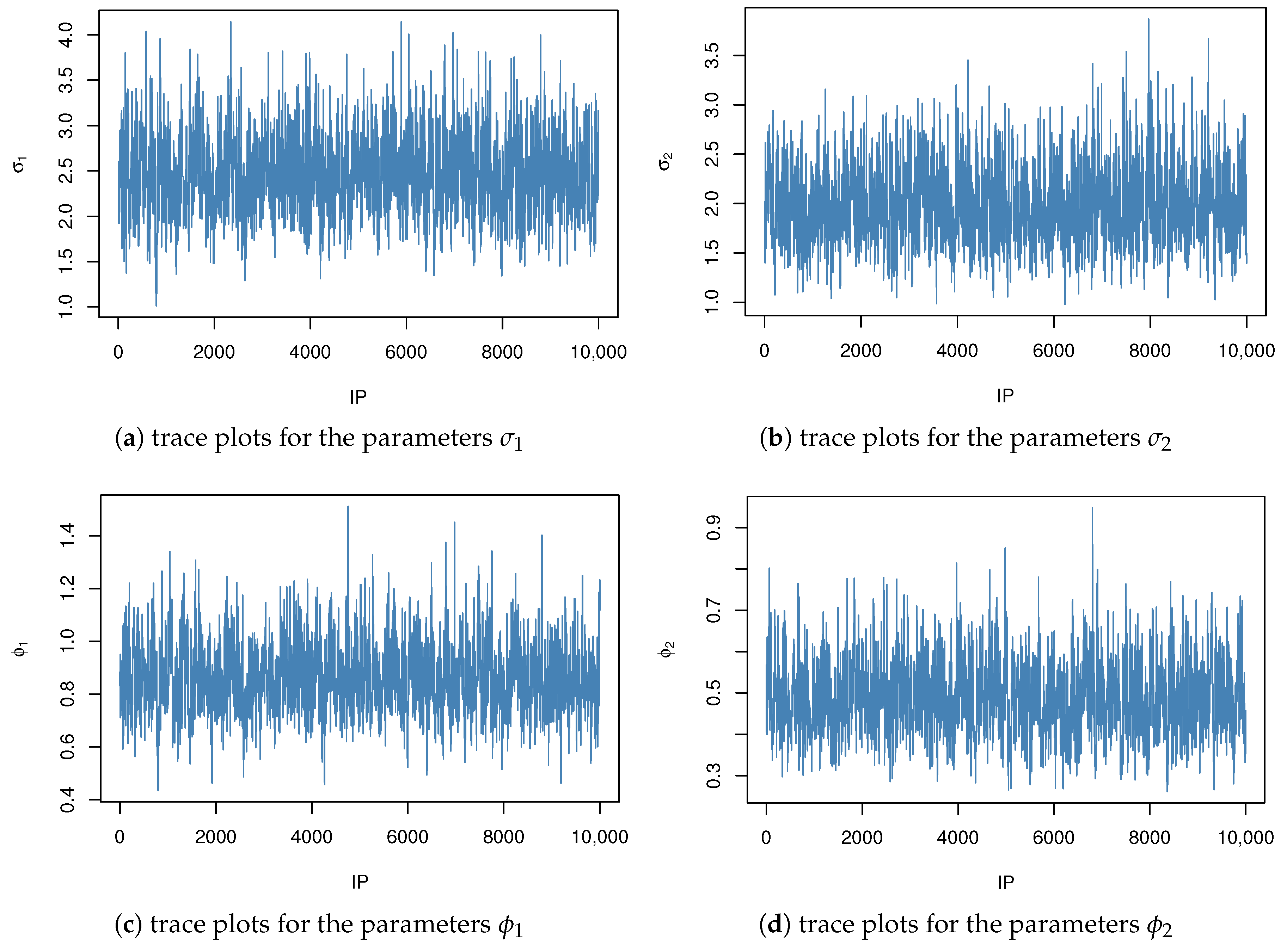
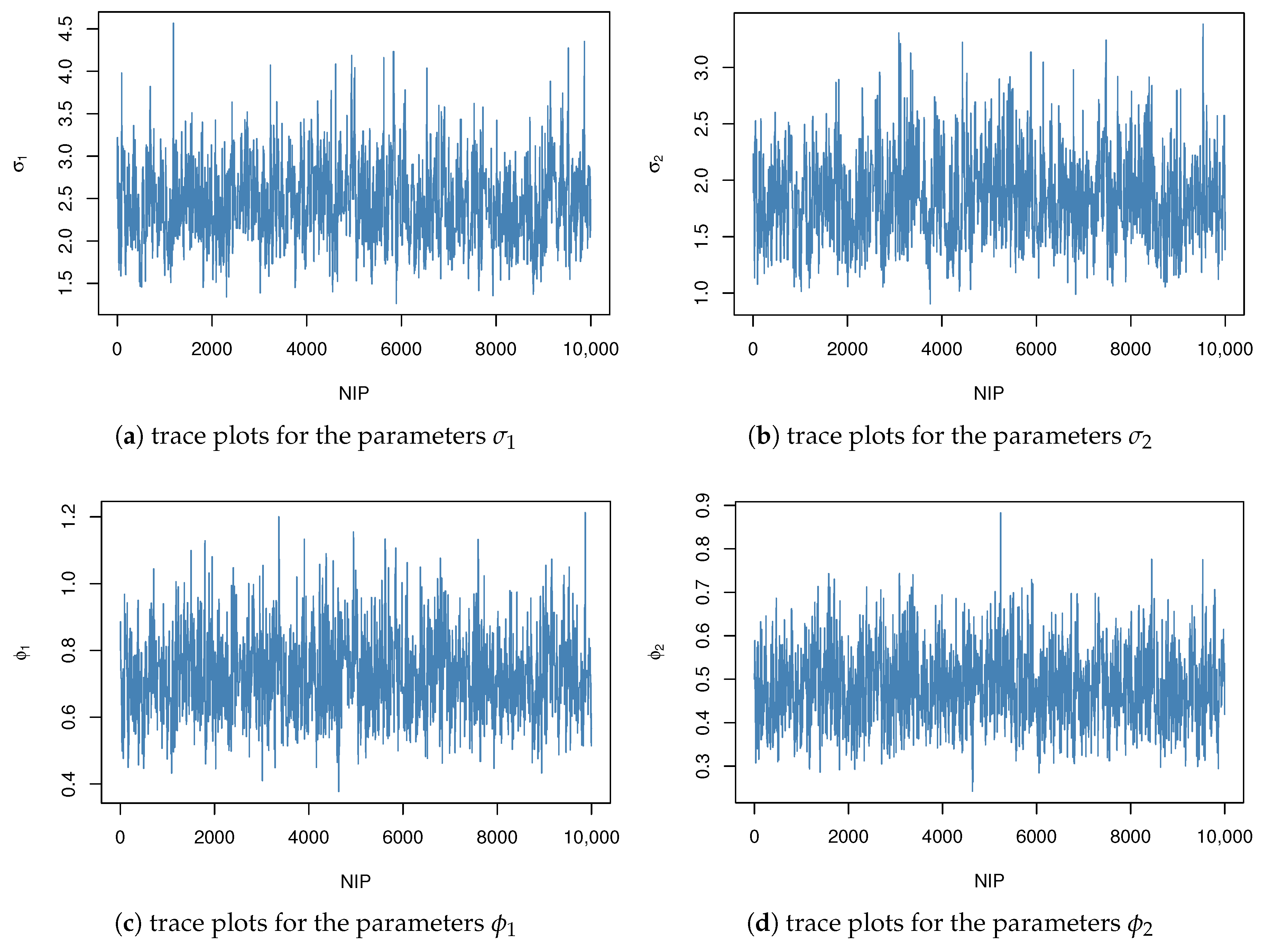
Through simulations, Bayes estimates and 95% CRIs for $({\sigma }_1,{\sigma }_2,{\varphi }_1,{\varphi }_2)$ are obtained via MCMC with 10,000 samples. Figure 4 and Figure 5 display the trace plots of the posterior samples under informative and non-informative priors, respectively. The convergence of the Markov chains was assessed using the Gelman–Rubin diagnostic, yielding a potential scale reduction factor of $\widehat{R}=1.01$. This value, being sufficiently close to 1, indicates satisfactory convergence and reliable mixing of the chains.

Table 1, Table 2, Table 3 and Table 4 reflect that the MSEs of the unknown parameter estimation become smaller as the sample size increases and the lengths of the confidence intervals also decrease. The MSEs of ${\widehat{\varphi }}_1$ and ${\widehat{\varphi }}_2$ are smaller than those of ${\widehat{\sigma }}_1$ and ${\widehat{\sigma }}_2$ in most cases. The confidence intervals of ${\varphi }_1$ and ${\varphi }_2$ are generally longer than those of ${\sigma }_1$ and ${\sigma }_2$. Among the two types of bootstrap confidence intervals, the approximate confidence intervals have a longer AL, while the bootstrap confidence intervals exhibit higher coverage probabilities. Furthermore, the Boot-T method demonstrates better accuracy than the Boot-P method, and we recommend using the Boot-T method for calculating confidence intervals.

From

Table 5. Bayesian estimations of parameter ${\sigma }_1$ with informative priors.

n	k	$({\mathit{R}}_1,\dots ,{\mathit{R}}_{\mathit{k}})$	SE		LINEX (l = −2)		LINEX (l = 2)
			ABE (MSE)	AL (CP)	ABE (MSE)	AL (CP)	ABE (MSE)	AL (CP)
30	25	(5, $0_{\left(24\right)}$)	2.3706	1.9878	2.3569	2.0109	2.3849	1.9627
			(1.8053)	(87.8%)	(1.7901)	(95.9%)	(1.8217)	(83.7%)
		($0_{\left(24\right)}$, 5)	2.3833	1.9531	2.3925	2.0099	2.3835	1.9918
			(1.8147)	(85.7%)	(1.8598)	(85.7%)	(1.8118)	(89.8%)
40	30	(10, $0_{\left(29\right)}$)	2.4067	2.0294	2.3655	1.9962	2.3640	2.0139
			(1.7942)	(98.0%)	(1.8229)	(89.8%)	(1.7905)	(95.9%)
		($0_{\left(29\right)}$, 10)	2.3724	1.9715	2.3651	2.0133	2.4026	1.9853
			(1.8223)	(87.8%)	(1.7948)	(93.9%)	(1.8275)	(91.8%)
50	35	(15, $0_{\left(34\right)}$)	2.3872	1.9961	2.3685	2.0010	2.3686	1.9972
			(1.8167)	(87.8%)	(1.7764)	(95.9%)	(1.7861)	(98.0%)
		($0_{\left(34\right)}$, 15)	2.3564	2.0290	2.3775	2.0517	2.3840	1.9875
			(1.8087)	(95.9%)	(1.8136)	(91.8%)	(1.8098)	(89.8%)
60	45	(15, $0_{\left(44\right)}$)	2.3806	1.9789	2.3584	1.9950	2.4154	1.9770
			(1.8084)	(89.8%)	(1.8160)	(91.8%)	(1.8094)	(87.8%)
		($0_{\left(44\right)}$, 15)	2.3754	1.9969	2.3647	2.0232	2.3874	2.0168
			(1.8207)	(93.9%)	(1.8259)	(91.8%)	(1.8140)	(93.9%)
70	45	(25, $0_{\left(44\right)}$)	2.3429	1.9811	2.3636	2.0173	2.3976	2.0244
			(1.8270)	(87.8%)	(1.8048)	(89.8%)	(1.8221)	(93.9%)
		($0_{\left(44\right)}$, 25)	2.3851	1.9612	2.3839	2.0105	2.3578	1.9927
			(1.8371)	(81.6%)	(1.8014)	(89.8%)	(1.7925)	(93.9%)
80	60	(20, $0_{\left(59\right)}$)	2.4105	2.0370	2.4011	2.0281	2.3270	2.0077
			(1.8123)	(98.0%)	(1.8060)	(93.9%)	(1.8104)	(93.9%)
		($0_{\left(59\right)}$, 20)	2.3922	2.0019	2.3880	2.0359	2.3535	2.0046
			(1.7996)	(93.9%)	(1.7931)	(100.0%)	(1.8276)	(89.8%)
90	55	(35, $0_{\left(54\right)}$)	2.3883	1.9870	2.3997	1.9721	2.3608	1.9372
			(1.8114)	(81.6%)	(1.8126)	(79.6%)	(1.8335)	(81.6%)
		($0_{\left(54\right)}$, 35)	2.3641	1.9804	2.3587	1.9813	2.3576	1.9955
			(1.8267)	(85.7%)	(1.8140)	(89.8%)	(1.7892)	(93.9%)
100	75	(25, $0_{\left(74\right)}$)	2.3844	2.0039	2.4292	2.0181	2.4165	1.9943
			(1.8122)	(87.8%)	(1.8047)	(93.9%)	(1.7967)	(87.8%)
		($0_{\left(74\right)}$, 25)	2.3622	1.9572	2.3761	1.9881	2.3792	2.0566
			(1.8148)	(81.6%)	(1.8018)	(85.7%)	(1.7800)	(98.0%)

,

Table 6. Bayesian estimations with informative priors of parameter ${\sigma }_2$.

n	k	$({\mathit{R}}_1,\dots ,{\mathit{R}}_{\mathit{k}})$	SE		LINEX (l = −2)		LINEX (l = 2)
			ABE (MSE)	AL (CP)	ABE (MSE)	AL (CP)	ABE (MSE)	AL (CP)
30	25	(5, $0_{\left(24\right)}$)	1.8875	1.9492	1.8926	1.9724	1.8844	1.9653
			(1.0156)	(91.8%)	(0.9887)	(98.0%)	(1.0282)	(98.0%)
		($0_{\left(24\right)}$, 5)	1.8946	1.9290	1.8725	2.0123	1.9212	1.9978
			(0.9879)	(91.8%)	(1.0508)	(95.9%)	(1.0206)	(98.0%)
40	30	(10, $0_{\left(29\right)}$)	1.8948	2.0151	1.9050	2.0204	1.8844	2.0149
			(1.0012)	(100.0%)	(1.0140)	(95.9%)	(0.9911)	(100.0%)
		($0_{\left(29\right)}$, 10)	1.8824	1.9656	1.8815	2.0288	1.8916	1.9722
			(1.0187)	(91.8%)	(1.0149)	(100.0%)	(1.0210)	(93.9%)
50	35	(15, $0_{\left(34\right)}$)	1.8482	1.9808	1.8844	2.0234	1.8774	2.0113
			(1.0042)	(93.9%)	(1.0304)	(95.9%)	(0.9986)	(98.0%)
		($0_{\left(34\right)}$, 15)	1.9010	2.0402	1.8738	2.0169	1.8735	1.9824
			(1.0364)	(100.0%)	(1.0368)	(93.9%)	(1.0054)	(100.0%)
60	45	(15, $0_{\left(44\right)}$)	1.8693	1.9875	1.8880	1.9782	1.8837	2.0129
			(1.0018)	(98.0%)	(0.9965)	(98.0%)	(1.0022)	(98.0%)
		($0_{\left(44\right)}$, 15)	1.8958	1.9744	1.8989	2.0729	1.8922	1.9971
			(1.0151)	(93.9%)	(1.0396)	(100.0%)	(1.0154)	(98.0%)
70	45	(25, $0_{\left(44\right)}$)	1.8703	1.9665	1.8809	2.0291	1.8897	2.0200
			(1.0079)	(93.9%)	(1.0109)	(100.0%)	(1.0123)	(98.0%)
		($0_{\left(44\right)}$, 25)	1.8725	2.0063	1.8855	2.0388	1.8946	1.9685
			(1.0420)	(93.9%)	(1.0238)	(98.0%)	(1.0037)	(98.0%)
80	60	(20, $0_{\left(59\right)}$)	1.9062	2.0586	1.8902	2.0279	1.9030	2.0047
			(1.0266)	(98.0%)	(1.0090)	(100.0%)	(1.0046)	(98.0%)
		($0_{\left(59\right)}$, 20)	1.8809	2.0273	1.8532	2.0703	1.8863	2.0016
			(1.0086)	(100.0%)	(1.0187)	(98.0%)	(1.0116)	(98.0%)
90	55	(35, $0_{\left(54\right)}$)	1.8851	2.0098	1.8965	2.0167	1.8845	1.9437
			(1.0148)	(93.9%)	(1.0143)	(100.0%)	(1.0269)	(91.8%)
		($0_{\left(54\right)}$, 35)	1.8668	2.0085	1.8766	1.9610	1.8649	2.0062
			(1.0190)	(98.0%)	(1.0224)	(95.9%)	(1.0017)	(100.0%)
100	75	(25, $0_{\left(74\right)}$)	1.8450	2.0107	1.9055	1.9823	1.8894	1.9754
			(1.0177)	(98.0%)	(1.0089)	(98.0%)	(1.0061)	(98.0%)
		($0_{\left(74\right)}$, 25)	1.9007	1.9878	1.9079	2.0002	1.8853	2.0553
			(1.0056)	(98.0%)	(1.0230)	(91.8%)	(1.0184)	(98.0%)

,

Table 7. Bayesian estimations with informative priors of parameter ${\varphi }_1$.

n	k	$({\mathit{R}}_1,\dots ,{\mathit{R}}_{\mathit{k}})$	SE		LINEX (l = −2)		LINEX (l = 2)
			ABE (MSE)	AL (CP)	ABE (MSE)	AL (CP)	ABE (MSE)	AL (CP)
30	25	(5, $0_{\left(24\right)}$)	0.7880	1.9348	0.7798	1.9250	0.7474	1.9634
			(1.0350)	(100.0%)	(1.0467)	(100.0%)	(1.0518)	(100.0%)
		($0_{\left(24\right)}$, 5)	0.7648	1.9585	0.7282	2.0310	0.7590	2.0200
			(1.0662)	(100.0%)	(1.0861)	(100.0%)	(1.1018)	(100.0%)
40	30	(10, $0_{\left(29\right)}$)	0.7454	2.0104	0.7727	1.9925	0.7675	2.0267
			(1.1104)	(100.0%)	(1.1131)	(100.0%)	(1.1220)	(100.0%)
		($0_{\left(29\right)}$, 10)	0.7503	1.9547	0.7503	2.0372	0.7306	2.0019
			(1.0623)	(100.0%)	(1.1095)	(100.0%)	(1.0935)	(98.0%)
50	35	(15, $0_{\left(34\right)}$)	0.7732	1.9844	0.7571	2.0098	0.7868	2.0362
			(1.0696)	(100.0%)	(1.1248)	(98.0%)	(1.1559)	(100.0%)
		($0_{\left(34\right)}$, 15)	0.7655	2.0171	0.7482	2.0284	0.7407	1.9685
			(1.0927)	(100.0%)	(1.1338)	(100.0%)	(1.0656)	(100.0%)
60	45	(15, $0_{\left(44\right)}$)	0.7669	1.9925	0.7896	1.9867	0.7769	2.0200
			(1.0812)	(100.0%)	(1.0683)	(100.0%)	(1.1238)	(100.0%)
		($0_{\left(44\right)}$, 15)	0.7575	1.9975	0.7604	2.0553	0.7359	2.0259
			(1.0883)	(100.0%)	(1.1656)	(100.0%)	(1.1325)	(100.0%)
70	45	(25, $0_{\left(44\right)}$)	0.7585	1.9794	0.7986	2.0585	0.7363	1.9880
			(1.0762)	(100.0%)	(1.1346)	(100.0%)	(1.0573)	(100.0%)
		($0_{\left(44\right)}$, 25)	0.7556	1.9790	0.7527	2.0220	0.7787	1.9494
			(1.0791)	(100.0%)	(1.1155)	(100.0%)	(1.0441)	(100.0%)
80	60	(20, $0_{\left(59\right)}$)	0.7713	2.0628	0.7808	2.0273	0.7734	1.9702
			(1.1584)	(100.0%)	(1.1272)	(100.0%)	(1.0746)	(100.0%)
		($0_{\left(59\right)}$, 20)	0.7714	2.0183	0.7614	2.0267	0.7696	1.9885
			(1.1505)	(100.0%)	(1.1235)	(100.0%)	(1.0889)	(100.0%)
90	55	(35, $0_{\left(54\right)}$)	0.7820	2.0414	0.7774	1.9956	0.7567	1.9270
			(1.1226)	(100.0%)	(1.1087)	(100.0%)	(1.0319)	(100.0%)
		($0_{\left(54\right)}$, 35)	0.7600	2.0179	0.7578	2.0083	0.7585	2.0070
			(1.1075)	(100.0%)	(1.0990)	(100.0%)	(1.1149)	(100.0%)
100	75	(25, $0_{\left(74\right)}$)	0.7770	2.0042	0.7534	1.9274	0.7711	1.9729
			(1.0648)	(100.0%)	(1.0628)	(100.0%)	(1.0986)	(100.0%)
		($0_{\left(74\right)}$, 25)	0.7543	1.9758	0.7579	1.9636	0.7830	2.0365
			(1.0916)	(100.0%)	(1.0561)	(100.0%)	(1.1810)	(98.0%)

,

Table 8. Bayesian estimations with informative priors of parameter ${\varphi }_2$.

n	k	$({\mathit{R}}_1,\dots ,{\mathit{R}}_{\mathit{k}})$	SE		LINEX (l = −2)		LINEX (l = 2)
			ABE (MSE)	AL (CP)	ABE (MSE)	AL (CP)	ABE (MSE)	AL (CP)
30	25	(5, $0_{\left(24\right)}$)	0.4479	1.9257	0.4600	1.9231	0.4572	1.9414
			(1.4684)	(85.7%)	(1.4896)	(87.8%)	(1.4738)	(81.6%)
		($0_{\left(24\right)}$, 5)	0.4652	1.9735	0.4719	1.9926	0.4469	2.0078
			(1.5191)	(85.7%)	(1.4883)	(91.8%)	(1.5528)	(83.7%)
40	30	(10, $0_{\left(29\right)}$)	1.1826	1.9430	1.2566	1.8483	1.7095	2.1583
			(1.9641)	(89.8%)	(1.9984)	(87.8%)	(3.1390)	(77.6%)
		($0_{\left(29\right)}$, 10)	0.4642	1.9585	0.4622	1.9961	0.4521	2.0441
			(1.5065)	(83.7%)	(1.5483)	(91.8%)	(1.5917)	(77.6%)
50	35	(15, $0_{\left(34\right)}$)	0.4947	1.9923	0.4645	1.9829	0.4855	2.0243
			(1.5285)	(77.6%)	(1.5515)	(87.8%)	(1.5969)	(85.7%)
		($0_{\left(34\right)}$, 15)	0.4469	1.9958	0.4633	2.0448	0.4695	1.9515
			(1.5244)	(85.7%)	(1.5923)	(87.8%)	(1.4796)	(93.9%)
60	45	(15, $0_{\left(44\right)}$)	0.4812	1.9906	0.4806	2.0079	0.4830	2.0399
			(1.5298)	(89.8%)	(1.5134)	(87.8%)	(1.6055)	(77.6%)
		($0_{\left(44\right)}$, 15)	0.4669	2.0013	0.4800	1.9992	0.4656	2.0573
			(1.5531)	(87.8%)	(1.5883)	(81.6%)	(1.6348)	(79.6%)
70	45	(25, $0_{\left(44\right)}$)	0.4728	1.9896	0.4673	2.0317	0.4722	2.0388
			(1.5578)	(75.5%)	(1.6017)	(83.7%)	(1.5929)	(87.8%)
		($0_{\left(44\right)}$, 25)	0.4696	1.9851	0.4602	2.0375	0.4703	1.9711
			(1.5587)	(83.7%)	(1.5809)	(83.7%)	(1.5200)	(85.7%)
80	60	(20, $0_{\left(59\right)}$)	0.4538	2.0808	0.4735	2.0287	0.4835	1.9505
			(1.6758)	(85.7%)	(1.6105)	(83.7%)	(1.4896)	(83.7%)
		($0_{\left(59\right)}$, 20)	0.4690	2.0242	0.4838	2.0718	0.4754	1.9847
			(1.6261)	(81.6%)	(1.6318)	(79.6%)	(1.5594)	(75.5%)
90	55	(35, $0_{\left(54\right)}$)	0.4694	2.0570	0.4542	1.9968	0.4610	1.8924
			(1.6257)	(81.6%)	(1.5820)	(75.5%)	(1.4360)	(71.4%)
		($0_{\left(54\right)}$, 35)	0.4703	1.9970	0.4675	1.9870	0.4765	2.0203
			(1.5703)	(89.8%)	(1.5628)	(79.6%)	(1.5875)	(81.6%)
100	75	(25, $0_{\left(74\right)}$)	0.4628	2.0110	0.4881	1.9638	0.4818	1.9870
			(1.5309)	(85.7%)	(1.5678)	(79.6%)	(1.5910)	(69.4%)
		($0_{\left(74\right)}$, 25)	0.4686	2.0212	0.4752	1.9800	0.4614	2.0516
			(1.6371)	(71.4%)	(1.5257)	(77.6%)	(1.6719)	(79.6%)
30	25	(5, $0_{\left(24\right)}$)	1.5480	2.4161	2.1406	2.2678	1.3822	1.9860
			(2.5582)	(93.9%)	(3.0099)	(91.8%)	(2.2323)	(81.6%)
		($0_{\left(24\right)}$, 5)	0.9740	2.1737	1.2118	2.4941	1.0486	1.8009
			(2.6087)	(85.7%)	(2.8807)	(91.8%)	(2.0553)	(81.6%)

,

Table 9. Bayesian estimations with non-informative priors of parameter ${\sigma }_1$.

n	k	$({\mathit{R}}_1,\dots ,{\mathit{R}}_{\mathit{k}})$	SE		LINEX (l = −2)		LINEX (l = 2)
			ABE (MSE)	AL (CP)	ABE (MSE)	AL (CP)	ABE (MSE)	AL (CP)
40	30	(10, $0_{\left(29\right)}$)	1.5802	2.2157	1.9679	2.3116	2.0461	2.1743
			(2.8926)	(83.7%)	(2.9664)	(81.6%)	(2.4395)	(81.6%)
		($0_{\left(29\right)}$, 10)	1.1826	1.9430	1.2566	1.8483	1.7095	2.1583
			(1.9641)	(89.8%)	(1.9984)	(87.8%)	(3.1390)	(77.6%)
50	35	(15, $0_{\left(34\right)}$)	2.0364	2.1276	1.8784	2.0380	1.9556	1.9957
			(2.0326)	(91.8%)	(2.0586)	(89.8%)	(2.0271)	(85.7%)
		($0_{\left(34\right)}$, 15)	1.2620	1.9878	1.2813	2.0564	1.2774	1.8567
			(2.1944)	(81.6%)	(2.0441)	(89.8%)	(2.1299)	(79.6%)
60	45	(15, $0_{\left(44\right)}$)	2.3763	2.1051	2.0878	2.2377	1.9965	2.0624
			(2.2382)	(85.7%)	(2.4502)	(85.7%)	(2.0640)	(83.7%)
		($0_{\left(44\right)}$, 15)	1.6969	2.4695	1.5392	2.1008	1.6616	2.1552
			(4.3595)	(85.7%)	(2.4201)	(83.7%)	(2.1957)	(83.7%)
70	45	(25, $0_{\left(44\right)}$)	2.5795	1.9825	1.8766	1.9502	2.0660	2.1293
			(1.9408)	(87.8%)	(2.1106)	(83.7%)	(1.9873)	(91.8%)
		($0_{\left(44\right)}$, 25)	1.5641	2.1690	1.5234	2.0614	1.4464	1.9682
			(2.2550)	(83.7%)	(2.2066)	(83.7%)	(2.0991)	(85.7%)
80	60	(20, $0_{\left(59\right)}$)	2.5638	2.0324	2.1266	2.2319	2.3135	2.0225
			(2.0372)	(79.6%)	(2.0347)	(95.9%)	(1.9967)	(83.7%)
		($0_{\left(59\right)}$, 20)	2.2819	2.0182	1.9951	2.1394	2.2417	2.0213
			(1.9075)	(93.9%)	(2.2067)	(83.7%)	(1.9467)	(93.9%)
90	55	(35, $0_{\left(54\right)}$)	2.8416	2.0501	2.0294	2.1637	2.2163	2.1947
			(2.4197)	(77.6%)	(2.1808)	(87.8%)	(2.1531)	(87.8%)
		($0_{\left(54\right)}$, 35)	1.3816	2.1359	1.6369	2.0759	1.3802	2.2492
			(2.1415)	(89.8%)	(2.1863)	(85.7%)	(3.0085)	(81.6%)
100	75	(25, $0_{\left(74\right)}$)	2.2050	2.2135	2.2141	2.0697	2.3403	2.3228
			(2.4067)	(93.9%)	(1.9926)	(91.8%)	(2.3557)	(93.9%)
		($0_{\left(74\right)}$, 25)	1.8130	2.0423	2.2908	2.0489	1.9302	2.3302
			(2.1609)	(85.7%)	(2.0272)	(89.8%)	(2.3010)	(91.8%)

,

Table 10. Bayesian estimations with non-informative priors of parameter ${\sigma }_2$.

n	k	$({\mathit{R}}_1,\dots ,{\mathit{R}}_{\mathit{k}})$	SE		LINEX (l = −2)		LINEX (l = 2)
			ABE (MSE)	AL (CP)	ABE (MSE)	AL (CP)	ABE (MSE)	AL (CP)
30	25	(5, $0_{\left(24\right)}$)	0.6512	2.8148	0.5779	2.5144	0.4912	1.9148
			(3.3984)	(83.7%)	(3.1803)	(79.6%)	(1.5772)	(75.5%)
		($0_{\left(24\right)}$, 5)	0.6438	2.1090	0.4896	2.2453	0.4941	1.6468
			(2.0855)	(75.5%)	(1.8679)	(83.7%)	(1.4253)	(69.4%)
40	30	(10, $0_{\left(29\right)}$)	1.0125	2.3856	0.7517	2.4991	1.1160	2.0321
			(2.4615)	(83.7%)	(2.2943)	(81.6%)	(1.6874)	(75.5%)
		($0_{\left(29\right)}$, 10)	0.7295	2.2856	0.8338	2.0150	0.4120	2.1851
			(2.0327)	(75.5%)	(2.4617)	(75.5%)	(2.5866)	(73.5%)
50	35	(15, $0_{\left(34\right)}$)	1.1035	2.2661	1.2590	2.1191	1.3850	2.0064
			(1.5476)	(87.8%)	(1.4206)	(83.7%)	(1.2976)	(81.6%)
		($0_{\left(34\right)}$, 15)	0.9627	2.0268	0.7930	4.5499	0.8411	2.1328
			(1.4652)	(77.6%)	(88.5848)	(77.6%)	(1.9737)	(71.4%)
60	45	(15, $0_{\left(44\right)}$)	1.5447	2.2243	1.3361	2.3736	1.6022	2.1741
			(1.5815)	(83.7%)	(2.2295)	(75.5%)	(1.5872)	(79.6%)
		($0_{\left(44\right)}$, 15)	1.2562	2.4776	1.0900	1.8561	1.2437	2.2084
			(3.7060)	(81.6%)	(1.4444)	(67.3%)	(1.9102)	(77.6%)
70	45	(25, $0_{\left(44\right)}$)	1.6356	1.8767	1.3484	2.0276	1.5394	2.2038
			(1.1906)	(85.7%)	(1.3526)	(85.7%)	(1.4872)	(85.7%)
		($0_{\left(44\right)}$, 25)	0.9581	2.3929	0.8040	2.7215	1.3046	2.2503
			(2.1358)	(71.4%)	(3.5398)	(79.6%)	(1.7526)	(85.7%)
80	60	(20, $0_{\left(59\right)}$)	1.4555	2.1285	1.8331	2.4837	1.5015	2.0226
			(1.5293)	(81.6%)	(2.0484)	(89.8%)	(1.3559)	(75.5%)
		($0_{\left(59\right)}$, 20)	1.4416	2.3119	1.6495	2.7631	1.3011	1.9700
			(1.4618)	(91.8%)	(7.2290)	(81.6%)	(1.2386)	(83.7%)
90	55	(35, $0_{\left(54\right)}$)	1.6816	2.2086	1.4534	2.1392	2.1126	2.4930
			(1.6942)	(85.7%)	(1.4602)	(81.6%)	(1.9421)	(87.8%)
		($0_{\left(54\right)}$, 35)	1.1638	2.0438	1.0168	2.1000	1.1026	2.2612
			(1.5970)	(75.5%)	(1.5154)	(77.6%)	(2.3309)	(83.7%)
100	75	(25, $0_{\left(74\right)}$)	1.9207	2.3785	1.7564	2.2384	2.0291	2.5014
			(1.7997)	(91.8%)	(1.3402)	(91.8%)	(1.8733)	(89.8%)
		($0_{\left(74\right)}$, 25)	1.5856	2.2387	1.7320	1.9777	1.6083	2.3707
			(1.5562)	(85.7%)	(1.2846)	(83.7%)	(1.7390)	(85.7%)

,

Table 11. Bayesian estimations with non-informative priors of parameter ${\varphi }_1$.

n	k	$({\mathit{R}}_1,\dots ,{\mathit{R}}_{\mathit{k}})$	SE		LINEX (l = −2)		LINEX (l = 2)
			ABE (MSE)	AL (CP)	ABE (MSE)	AL (CP)	ABE (MSE)	AL (CP)
30	25	(5,$0_{\left(24\right)}$)	0.5353	3.3155	0.6271	2.4496	0.4466	2.0504
			(5.9485)	(89.8%)	(3.0924)	(91.8%)	(1.8537)	(85.7%)
		($0_{\left(24\right)}$, 5)	0.3596	2.0448	0.4148	2.1659	0.3818	1.5541
			(1.7986)	(81.6%)	(1.8183)	(87.8%)	(0.8629)	(77.6%)
40	30	(10, $0_{\left(29\right)}$)	0.5703	2.2868	0.6346	2.6119	0.6137	2.0293
			(1.9131)	(91.8%)	(2.9320)	(89.8%)	(1.2715)	(83.7%)
		($0_{\left(29\right)}$, 10)	0.4577	2.1353	0.4502	2.3382	0.5640	2.8423
			(1.7700)	(81.6%)	(3.0196)	(87.8%)	(5.1180)	(81.6%)
50	35	(15, $0_{\left(34\right)}$)	0.7506	2.3386	0.5878	2.5043	0.6626	1.9867
			(1.9390)	(93.9%)	(3.2049)	(98.0%)	(1.1317)	(100.0%)
		($0_{\left(34\right)}$, 15)	0.4686	2.2744	0.4756	8.3762	0.4703	2.0737
			(2.4263)	(93.9%)	(524.8768)	(93.9%)	(1.4771)	(89.8%)
60	45	(15, $0_{\left(44\right)}$)	0.7559	2.3059	0.6807	2.3589	0.6753	2.3938
			(1.5288)	(100.0%)	(1.9534)	(95.9%)	(2.0508)	(93.9%)
		($0_{\left(44\right)}$, 15)	0.5293	2.2191	0.5304	1.9785	0.5775	2.2061
			(3.5792)	(89.8%)	(1.0929)	(91.8%)	(1.8382)	(91.8%)
70	45	(25, $0_{\left(44\right)}$)	0.7655	1.9698	0.6136	1.9886	0.6646	2.6046
			(1.6379)	(91.8%)	(1.2671)	(91.8%)	(3.5672)	(93.9%)
		($0_{\left(44\right)}$, 25)	0.5200	2.6593	0.5470	2.8428	0.4743	2.4293
			(2.6459)	(93.9%)	(3.7688)	(93.9%)	(1.8846)	(95.9%)
80	60	(20, $0_{\left(59\right)}$)	0.7625	2.3931	0.6991	2.6065	0.7280	2.3116
			(2.2126)	(95.9%)	(2.5559)	(100.0%)	(1.5521)	(100.0%)
		($0_{\left(59\right)}$, 20)	0.7327	2.7273	0.6318	2.8801	0.7085	2.1452
			(3.0075)	(98.0%)	(7.8764)	(93.9%)	(1.8298)	(95.9%)
90	55	(35, $0_{\left(54\right)}$)	0.7656	2.3509	0.6789	2.2505	0.6980	2.6685
			(1.8887)	(98.0%)	(1.5355)	(98.0%)	(2.3452)	(98.0%)
		($0_{\left(54\right)}$, 35)	0.5117	2.3849	0.6026	2.0563	0.4903	2.3258
			(1.9807)	(91.8%)	(1.3804)	(91.8%)	(2.3637)	(91.8%)
100	75	(25, $0_{\left(74\right)}$)	0.6699	2.2491	0.7304	2.3597	0.7433	2.4315
			(1.8625)	(98.0%)	(1.6391)	(98.0%)	(2.0645)	(98.0%)
		($0_{\left(74\right)}$, 25)	0.6170	2.2390	0.7310	2.2152	0.6602	2.5509
			(1.5628)	(95.9%)	(1.5762)	(93.9%)	(2.7506)	(98.0%)

and

Table 12. Bayesian estimations with non-informative priors of parameter ${\varphi }_2$.

n	k	$({\mathit{R}}_1,\dots ,{\mathit{R}}_{\mathit{k}})$	SE		LINEX (l = −2)		LINEX (l = 2)
			ABE (MSE)	AL (CP)	ABE (MSE)	AL (CP)	ABE (MSE)	AL (CP)
30	25	(5, $0_{\left(24\right)}$)	0.1852	3.4119	0.1492	2.4245	0.1471	2.3968
			(2.1948)	(89.8%)	(3.2305)	(91.8%)	(3.4885)	(83.7%)
		($0_{\left(24\right)}$, 5)	0.1954	2.1659	0.1390	2.4238	0.1505	1.9482
			(2.6668)	(89.8%)	(3.5206)	(85.7%)	(2.6988)	(81.6%)
40	30	(10, $0_{\left(29\right)}$)	0.2510	2.3812	0.2255	2.3000	0.2784	1.8672
			(2.4263)	(85.7%)	(2.7101)	(93.9%)	(1.3863)	(79.6%)
		($0_{\left(29\right)}$, 10)	0.2088	2.0765	0.2346	2.1878	0.1332	2.7835
			(2.1543)	(79.6%)	(3.2283)	(85.7%)	(5.6957)	(83.7%)
50	35	(15, $0_{\left(34\right)}$)	0.2915	2.4930	0.3308	2.9080	0.3414	1.8737
			(2.6566)	(85.7%)	(5.1590)	(85.7%)	(1.3498)	(91.8%)
		($0_{\left(34\right)}$, 15)	0.2793	7.0613	0.2153	8.6163	0.2319	2.0166
			(4.7474)	(89.8%)	(6.7651)	(85.7%)	(1.7329)	(89.8%)
60	45	(15, $0_{\left(44\right)}$)	0.3823	2.1878	0.3682	2.3146	0.4475	2.4718
			(1.8401)	(89.8%)	(2.2453)	(85.7%)	(2.5356)	(83.7%)
		($0_{\left(44\right)}$, 15)	0.3607	2.6508	0.3143	2.0174	0.3344	2.0446
			(4.9544)	(93.9%)	(1.5417)	(87.8%)	(1.8418)	(93.9%)
70	45	(25, $0_{\left(44\right)}$)	0.3918	1.8636	0.3489	2.1973	0.3922	2.3914
			(1.5599)	(93.9%)	(2.0016)	(91.8%)	(2.3577)	(77.6%)
		($0_{\left(44\right)}$, 25)	0.2798	2.5979	0.2364	2.8163	0.3465	2.2074
			(2.9326)	(85.7%)	(4.1749)	(85.7%)	(2.0283)	(85.7%)
80	60	(20, $0_{\left(59\right)}$)	0.3736	2.2301	0.4164	2.6121	0.3821	2.3852
			(2.2010)	(79.6%)	(3.1024)	(75.5%)	(2.1156)	(91.8%)
		($0_{\left(59\right)}$, 20)	0.3677	2.8879	0.4022	2.9638	0.3387	2.3281
			(4.9485)	(93.9%)	(8.9474)	(83.7%)	(2.5006)	(91.8%)
90	55	(35, $0_{\left(54\right)}$)	0.4090	2.3874	0.3776	2.3019	0.4601	2.8951
			(2.3146)	(91.8%)	(2.2812)	(81.6%)	(3.8582)	(77.6%)
		($0_{\left(54\right)}$, 35)	0.3161	2.4162	0.2770	2.1250	0.3104	2.4059
			(2.3661)	(85.7%)	(2.0055)	(85.7%)	(2.8522)	(93.9%)
100	75	(25, $0_{\left(74\right)}$)	0.4527	2.2345	0.4505	2.2470	0.4632	2.5819
			(2.2973)	(83.7%)	(1.9727)	(81.6%)	(2.6491)	(73.5%)
		($0_{\left(74\right)}$, 25)	0.4078	2.4246	0.4341	2.1522	0.4076	2.5533
			(2.2765)	(79.6%)	(1.8750)	(93.9%)	(3.1466)	(91.8%)

, it can be seen that in the Bayesian statistical method, across different censoring schemes, the MSEs of the unknown parameter estimates remain relatively consistent, indicating that variations in censoring schemes have minimal impact on estimation accuracy. Additionally, the estimates of ${\varphi }_1$ and ${\varphi }_2$ exhibit relatively small biases and MSEs, suggesting that these parameters are estimated with high accuracy and stability. In contrast, ${\sigma }_1$ consistently has the highest MSE, indicating greater uncertainty in its estimation, which may require more refined methods to improve precision. When comparing estimation methods, the SE and LINEX methods yield similar MSEs and ALs. Furthermore, MLEs exhibit lower biases and MSEs than Bayesian estimates and demonstrate greater stability across different censoring schemes, further highlighting their superiority in practical applications. Regarding the Bayesian estimates with non-informative priors, as the sample size increases, we observe that the MSE decreases and the coverage rate increases. However, the results do not outperform those obtained using informative priors. This finding underscores the importance of selecting appropriate priors in Bayesian inference to achieve optimal results.

5.2. Real Data Analysis

This section presents an analysis of the real dataset to illustrate the practical application of the proposed methods.

The first dataset represents the breakdown times of an insulating fluid between electrodes at a voltage of 34 kV, measured in minutes. This dataset, sourced from [23], is widely used in reliability analysis and serves as a standard example for studying the breakdown behavior of insulating materials under controlled electrical stress.

The second dataset records the time in months to the first failure of various small electric carts used for internal transportation and delivery within a large manufacturing facility. This dataset, which was initially sourced from Zimmer [24], provides valuable real-world failure data for mechanical systems in industrial environments, making it particularly relevant to our analysis of system reliability in operational settings.

Hasaballah [21] also analyzes these data. To conform with the assumptions of this study, only the first 19 failure times are utilized. The dataset provided in

Table 13. Breakdown times of two datasets.

Breakdown times of 19 devicest in hours	0.19	0.78	0.96	1.31	2.78	3.16	4.15
	4.76	4.85	6.5	7.35	8.01	8.27	12.06
	31.75	32.52	33.91	36.71	72.89
Breakdown times of 20 electronic carts in months	0.9	1.5	2.3	3.2	3.9	5.0	6.2
	7.5	8.3	10.4	11.1	12.6	15.0	16.3
	19.3	22.6	24.8	31.5	38.1	53.0

comprises the following.

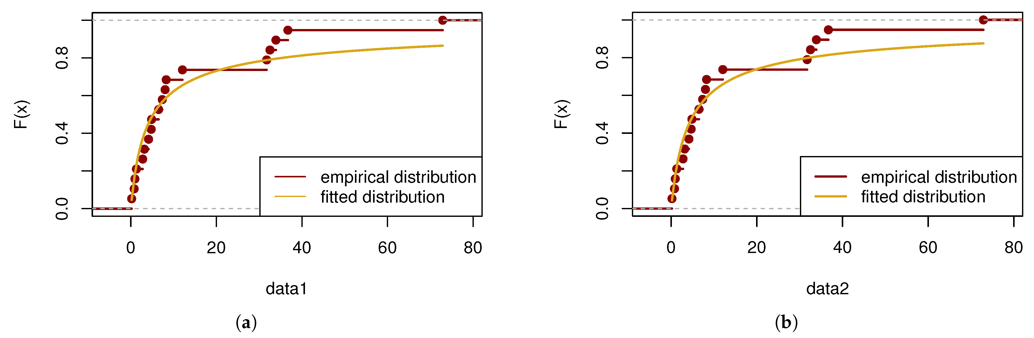
In this part, a goodness-of-fit test is performed using the Kolmogorov–Smirnov (K-S) statistic. The calculated p value for the first sample is 0.7998, while for the second sample, the p value is 0.5906. The results of the test are visually presented in Figure 6.

Using Algorithm 5 to analyze real data, the following statistical inferences were obtained.

$$R=(0,0,0,0,1,1,1,1,0,0,0,0,0,0)$$

Among the various censoring schemes, the one described above achieves the smallest MSEs for ${\widehat{\sigma }}_1$, ${\widehat{\sigma }}_2$, ${\widehat{\varphi }}_1$, and ${\widehat{\varphi }}_2$, along with the highest accuracy.

Algorithm 5 Pseudocode for classical statistical and Bayesian estimation methods on real data

1: Perform Kolmogorov-Smirnov (K-S) test to verify if both populations follow Lomax distribution. 2: Set $n=19$ and R. Generate the B-JPC sample from Lomax distribution in Algorithm 4. 3: Calculate the likelihood function based on Fnction (3). 4: Use R language’s ‘optim’ function to compute the MLE for the parameters. 5: Compute the Fisher information matrix and take its inverse to obtain the covariance matrix for the ACI. 6: Set a gamma prior such that the prior mean is close to the MLE estimate. Apply Algorithm 3 to compute the Bayesian estimate using the information prior.

Using the MLE method, we estimate ${\sigma }_1$, ${\sigma }_2$, ${\varphi }_1$, and ${\varphi }_2$ based on the data type in this study. The results are summarized in

Table 14. Real data analysis.

	AMLE (Var)	LOWRE (UPPER)	SE		LINEX (l = −2)		LINEX (l = 2)
			BAS	AL	BAS	AL	BAS	AL
${\sigma }_1$	2.4688 (0.5916)	1.5592 (4.0661)	2.1522	2.0045	2.1548	1.9898	2.1503	1.9978
${\sigma }_2$	3.3280 (0.4052)	2.4688 (4.3792)	2.5460	2.0034	2.5543	1.9859	2.5514	2.0848
${\varphi }_1$	0.5347 (0.3163)	0.3052 (1.0078)	0.5636	2.0224	0.5685	1.9591	0.5592	2.1329
${\varphi }_2$	0.4588 (0.3268)	0.2735 (0.7630)	0.4152	2.0583	0.4040	2.0068	0.4114	2.0960

.

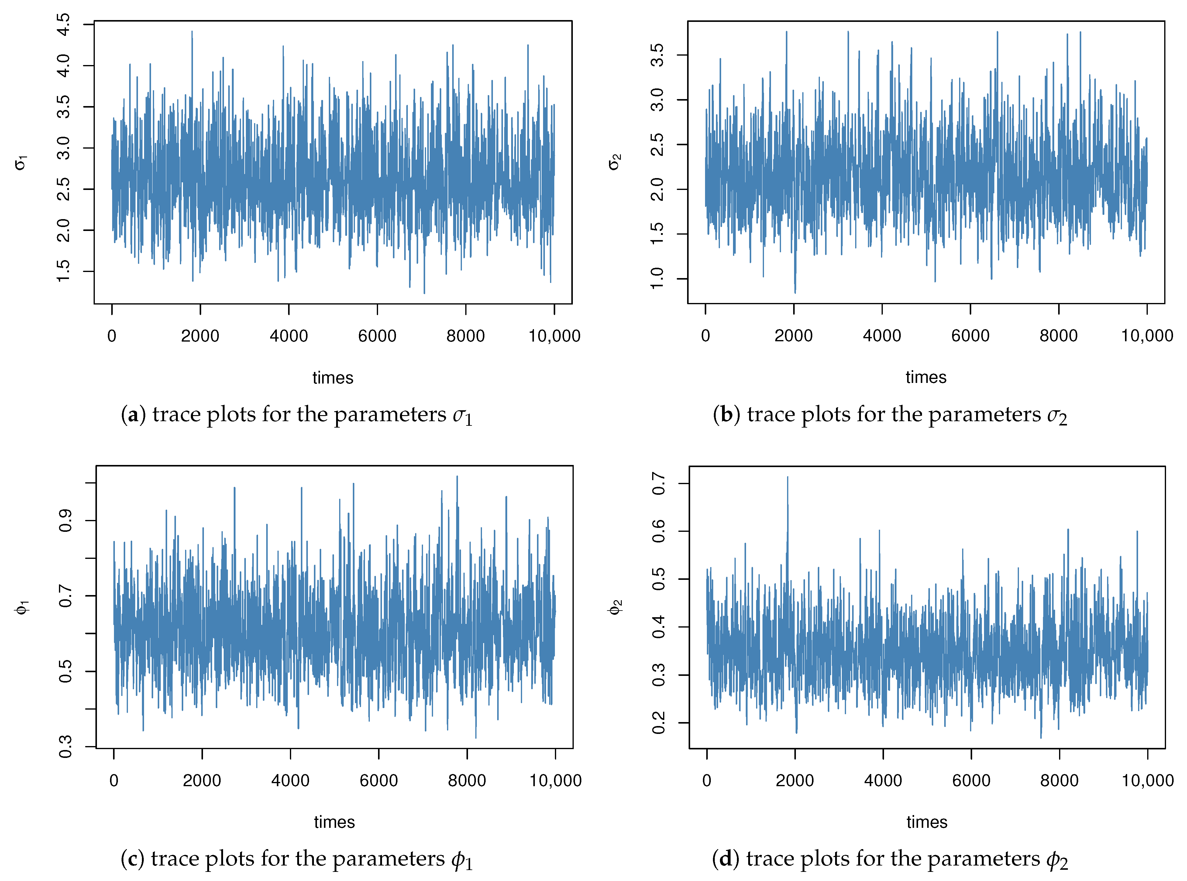
For Bayesian estimation, the MCMC method is implemented with 10,000 iterations.The Bayesian estimates of ${\sigma }_1,{\sigma }_2,{\varphi }_1$, and ${\varphi }_2$ are computed under both SE and LINEX loss functions, with the results summarized in Table 14. Figure 7 displays the trace plots of the posterior samples under informative priors.

The data indicate that the AMLE values are reasonable and closely align with previous studies. Additionally, our method produces narrower 95% confidence intervals, which highlights its advantages in practical applications. Furthermore, the Bayesian estimates calculated using two different loss functions are quite similar, demonstrating the robustness of our method.

6. Conclusions

This study employs both maximum likelihood estimation and Bayesian inference to estimate unknown parameters under the B-JPC framework. Since explicit MLE solutions and closed-form Bayesian estimators are unavailable, numerical methods are utilized alongside Gamma priors to facilitate parameter estimation. The Markov Chain Monte Carlo method is implemented under both squared error and linear exponential loss functions, ensuring a comprehensive analysis of parameter behavior under different estimation criteria.

To validate the proposed methods, real datasets are analyzed, and extensive simulation studies are conducted to assess their performance across varying sample sizes. The results indicate that as the sample size increases, the MSEs of the unknown parameters decrease, and the lengths of the confidence intervals shorten accordingly. When comparing the two types of bootstrap confidence intervals, the Boot-T method demonstrates better accuracy, and it is recommended for practical use. The Bayesian method shows stability across different censoring schemes. Although Bayesian estimates with non-informative priors improve as the sample size increases, they are still less precise compared to those obtained with informative priors. This finding emphasizes the importance of selecting appropriate priors in Bayesian inference to achieve more accurate estimation results.

Moving forward, this research will be extended to two distinct populations characterized by different Lomax distribution parameters and sample sizes. Additionally, sensitivity analysis will be conducted for the Bayesian statistical inference, further enhancing the robustness of the results. This study aims to explore parameter estimation under a balanced joint progressive Type-II censoring scheme, further expanding the applicability of comparative lifetime experiments. A comprehensive comparison between traditional methods and the BJPC method, including performance metrics such as accuracy, efficiency, and robustness, is a valuable next step.