The Linear Stability of a Power-Law Liquid Film Flowing Down an Inclined Deformable Plane

Abstract

A linear stability analysis is performed for a power-law liquid film flowing down an inclined rigid plane over a deformable solid layer. The deformable solid is modeled using a neo-Hookean constitutive equation, characterized by a constant shear modulus and a nonzero first normal stress difference in the base state at the fluid–solid interface. To solve the linearized eigenvalue problem, the Riccati transformation method, which offers advantages over traditional techniques by avoiding the parasitic growth seen in the shooting method and eliminating the need for large-scale matrix eigenvalue computations, was used. This method enhances both analytical clarity and computational efficiency. Results show that increasing solid deformability destabilizes the flow at low Reynolds numbers by promoting short-wave modes, while its effect becomes negligible at high Reynolds numbers where inertia dominates. The fluid’s rheology also plays a key role: at low Reynolds numbers, shear-thinning fluids ($n<1$) are more prone to instability, whereas at high Reynolds numbers, shear-thickening fluids ($n>1$) exhibit a broader unstable regime.

1. Introduction

Instability in thin films and layered systems has garnered widespread attention due to its relevance in various engineering and scientific applications, such as coating processes, lubrication systems, and fuel spraying. In such applications, the stability of the interface and its morphology play a crucial role in determining performance efficiency. Although traditional studies have mostly focused on solid substrates, there is an increasing need to understand the effect of flexible or deformable substrates on the emergence and development of surface instability patterns. This issue is particularly significant in modern technologies such as flexible electronics, bendable solar cells, and optomechanical sensor devices, where the substrate is not merely a passive element but actively participates in the system’s mechanical response.

In this context, surface undulations and structural buckling are not only viewed as undesirable deformations but are also harnessed to enhance light efficiency in organic devices, increase material flexibility, and improve resistance to repeated mechanical loads. However, most previous analytical studies and numerical models have relied on idealized assumptions, often neglecting the possibility of synchronization between surface wrinkling and global buckling. In this regard, the work of Nikravesh et al. [1] offered significant insights by employing direct numerical simulations to investigate the transition from surface wrinkling to global buckling in thin films on compliant substrates, revealing complex nonlinear interactions that govern these instabilities.

In fact, there are many studies devoted to investigating the stability of a power-law liquid film flowing down an inclined plane. It should be noted that most of these studies have developed a Benney-type free surface evolution equation [2], employing the classical long-wave expansion. This approach, based on the lubrication approximation, is quite appropriate for capturing long-wave instabilities only. With such models, the amplitude of waves is greatly underestimated above the instability threshold. Although the Benney equation contains various physical mechanisms and is likely to describe nonlinear behavior close to the instability threshold, it loses its physical relevance when convective effects become significant, due to the production of shorter wave components [3]. To fill this gap, our study focuses on capturing both long- and short-wave instabilities by employing a numerical approach based on the Riccati method, which allows us to resolve singularities in the Orr–Sommerfeld equations and accurately model the nonlinear and convective effects in power-law liquid films over deformable substrates.

Motivated by these findings, the present study aims to explore similar behaviors using an efficient numerical framework based on the embedded defect technique, thereby contributing to the understanding and design of advanced functional materials with tailored mechanical responses.

The flow of thin-film Newtonian or non-Newtonian fluids over a layer of deformable solids has been the subject of relatively few studies in the past. We chose to focus on this area in order to capture the interfacial and surface waves. Moreover, to do this, we opted for a numerical study based on Riccati matrices. In the classical case of Newtonian or non-Newtonian films falling onto a solid substrate, it is known that the flow becomes unstable at long-wavelength perturbations when the destabilizing effect of inertia outweighs the stabilizing effect of gravity [4,5]. A novelty of our study lies in the presence of the deformable solid, which generates short waves at the free surface of the fluid. We have shown that these short waves persist even when the fluid is Newtonian, i.e., $n=1$. This explains how the deformability of the solid layer affects the instability of the free surface.

Seminal works of Benjamin [4] and Yih [6] on the linear stability of thin films gave rise to further research in this area. These studies have examined the stability of Newtonian and non-Newtonian fluid flows [7,8,9], as well as the variation in the physical properties of isothermal and non-isothermal systems [10,11], such as surface tension and thermal diffusivity. In addition to the instabilities observed in a single-phase problem [12], in two-phase flows, instability can result from viscosity stratification, density stratification, or from shear effects [13,14]. Recent results in this line of research represent significant progress, which is important for both practical applications and theory. Coating involves applying thin liquid layers onto a moving substrate, understood by analyzing fluid mechanical components like the boundary layer, wetting line, withdrawal, and others. Although some aspects are well studied, others need further investigation. Despite limitations in predictive modeling, advancements in coating science, as shown in [15], offer valuable insights for design and practical uses (see, e.g., [16] for a discussion of recent advances in problems on flexible-tube flows and their physiological applications). The typical applications vary from cardiovascular system phenomena like wave propagation and flow-induced instabilities; respiratory system aspects including phonation and airway dynamics [17]; and other applications like peristaltic transport [18].

To enrich the contextual and methodological framework of the present study on fluid–structure interactions and interface dynamics, recent contributions provide valuable insights into multi-physics and multiphase systems. For instance, a study on nonlinear free vibrations of nanocomposite micropipes conveying laminar flow under thermal effects explores the impact of external forces like heat on fluid–structure dynamics, while another develops a thermodynamically consistent phase-field lattice Boltzmann method for simulating two-phase electrohydrodynamic flows, offering a robust framework for multi-physics interactions [19,20]. In addition, research on isolated slug dynamics in voided pipelines sheds light on impact behavior and fluid discontinuities, complementing the investigation of multiphase flow [21]. Furthermore, advanced techniques such as three-dimensional bubble geometry reconstruction using a ray tracing algorithm enhance interface tracking precision in multiphase systems, while studies on interfacial polymerization for nanofiltration membrane preparation deepen our understanding of molecular interactions and stability at fluid-deformable surface interfaces [22,23]. By incorporating these approaches, our study strengthens its methodology and places its findings within the broader scope of fluid–structure interactions and phase behavior modeling, improving the accuracy of computational and experimental analyses.

In [24], the authors investigate the influence of a deformable solid layer on the stability of liquid flow down an inclined plane. They find that the presence of a soft solid layer suppresses the free-surface instability, offering a potential passive method to control instabilities in liquid film flows. Building on this, Jain and Shankar [25] investigate the suppression of instabilities in viscoelastic film flows down an inclined plane with a deformable solid layer. Numerical simulations show suppression of the original instability with highly deformable solids and reveal the occurrence of new unstable modes. This study suggests using elastohydrodynamic coupling to control instabilities in viscoelastic film flows. Amaouche et al. [26] present a more detailed and sophisticated modeling approach compared to previous studies. Although earlier research was focused on the suppression of instability with deformable solid layers, this paper explores the complex modeling aspects of the flow of power-law fluids down an inclined plane. This approach accurately captures nonlinear behavior and provides insights into the convective nature of instability, unaffected by variations in the power-law index. Additionally, it introduces both full and reduced models, offering practical options for modeling complex fluid flow phenomena. In the lubrication approximation, Perazzo and Gratton [27] examined the family of traveling wave solutions describing the flow of a power-law liquid film on an inclined plane.

The Orr–Sommerfeld equation serves as a fundamental tool for examining linear stability in fluid mechanics. By introducing an infinitesimal disturbance to the laminar state, this equation enables the determination of neutral instability thresholds or perturbation growth rates for various Reynolds and wave numbers. For more detailed insights, see [28,29] and the references therein. In [30,31], the authors investigate the interplay between power-law liquid films and solid neo-Hookean layers. Understanding the dynamics of the liquid–solid interface is essential for gauging system stability.

The stability of liquid films flowing down inclined planes has been extensively studied, with significant attention given to both Newtonian and non-Newtonian fluids on rigid substrates (see [9,26,32] and the references therein). Recent advances have expanded this scope: for example, Pascal and Vacca [9] analyzed shear-thinning fluids over porous layers, while Noble and Vila [32] developed consistent shallow-water models for power-law films. However, fewer investigations have explored gravity-driven flows over deformable substrates [33,34,35,36], with Shankar and Sahu [24] notably demonstrating instability suppression by soft layers. Despite these efforts, a critical research gap remains: the stability of viscoelastic power-law film flows over deformable neo-Hookean solid layers is underexplored, particularly how substrate deformability influences instability thresholds and triggers new dynamic behaviors, which are crucial for applications in biological systems (e.g., blood flow in elastic vessels) and industrial processes (e.g., coating on compliant surfaces). In this paper, we investigate the stability of a power-law liquid film flowing down an inclined deformable plane, modeled with a neo-Hookean solid layer, addressing this gap through linear stability analysis and numerical solutions of Orr–Sommerfeld equations.

Our study uncovers novel insights: the deformable neo-Hookean layer significantly shifts the critical Reynolds and wave numbers at which instability begins, differing markedly from rigid-surface scenarios, and it introduces unique unstable modes driven by elastohydrodynamic coupling between the fluid and solid. Additionally, by applying the Riccati method, we overcome singularities in Orr–Sommerfeld equations caused by viscosity divergence at the free surface, a challenge unresolved in prior works like [9,32], delivering a more precise stability analysis than previous approaches.

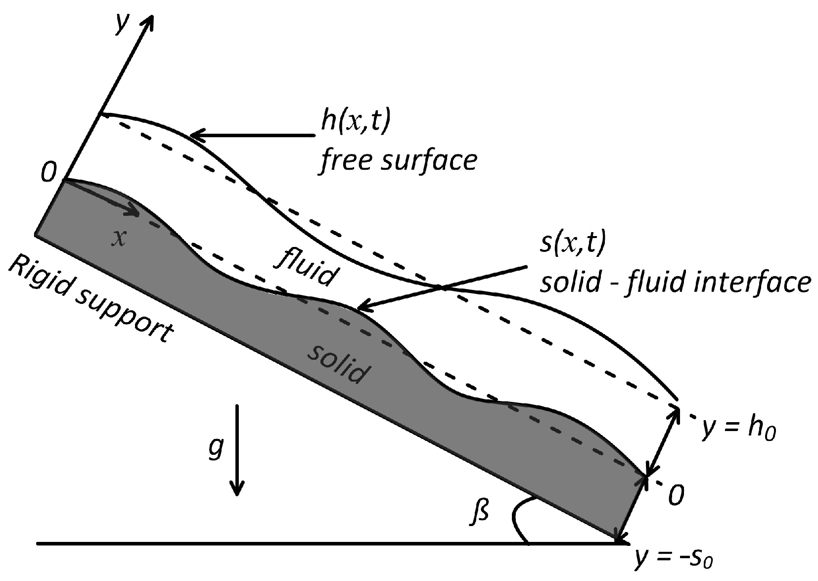
This paper is organized as follows. The governing equations, base state, characteristic scales and non-dimensional equations are presented in Section 2, where we also introduce the Orr–Sommerfeld equation as a result of the linear stability analysis. In Section 3, the solution methodology is presented and discussed. The main numerical results are discussed in Section 4, where we also include a comparison with results presented in the literature. Finally, in Section 5, our conclusions and plans for the future are discussed.

2. Problem Formulation

The physical model shown in Figure 1 features a thin film of a power-law liquid flowing down the surface of an incompressible deformable solid under the influence of gravity $\mathbf{g}$ and surface tension. The solid is fixed onto a rigid inclined plane making an angle $\beta$ with the horizontal. A Cartesian frame of reference $(x,y)$ is adopted, where x and y are directions along the longitudinal and perpendicular planes, respectively, to the initial unperturbed surface of the solid layer $(y=0)$.

The interface between the solid and fluid is represented by $y=s(x,t)$, while the interface between the fluid and a passive gas is given by $y=h(x,t)$. In the unperturbed state, these interfaces are located at $y=0$ and $y=h_0$, respectively. The rigid plate is positioned at $y=-s_0$. The fluid and the solid layer occupy the regions $0\le y\le h_0$ and $-s_0\le y\le 0$, respectively. A sketch of the hydrodynamical system considered is shown in Figure 1.

2.1. Governing Equations

The fluid flow is governed by the standard two-dimensional incompressible Navier–Stokes equations (see, e.g., Malvern [37]):

$$\begin{array}{ccc}\hfill {\rho }_f\left({\displaystyle \frac{\partial \mathbf{v}}{\partial t}}+\mathbf{v}·\mathsf{\nabla }\mathbf{v}\right)& =& -\mathsf{\nabla }p+div\mathit{\tau }+{\rho }_f\mathit{g},\hfill \end{array}$$

(1)

$$\begin{array}{ccc}\hfill div\mathbf{v}& =& 0,\hfill \end{array}$$

(2)

Equation (1) represents the Navier–Stokes momentum equation for the power-law fluid, showing how fluid acceleration (left side) is balanced by pressure gradients, viscous stresses (via the stress tensor $\mathit{\tau }$), and gravity, driving the flow down the inclined plane. We focus on the incompressible case, simplifying to Equation (2).

Equation (2) represents the continuity equation for incompressible fluids, while ${\displaystyle \frac{\partial {\rho }_f}{\partial t}}+div\left({\rho }_f\mathbf{v}\right)=0$ represents the compressible case. Both forms ensure continuity, where $\mathbf{v}=(u,v)$ is the flow velocity, p is the pressure and ${\rho }_f$ is the density of the fluid. In (1), $\mathit{\tau }$ stands for the stress tensor, which can be written as follows:

$$\mathit{\tau }=K\eta \left(\mathsf{\nabla }\mathbf{v}+\mathsf{\nabla }{\mathbf{v}}^T\right),$$

where $\eta ={\left\{2(u_{,x}^2+v_{,y}^2)+{(u_{,y}+v_{,x})}^2\right\}}^{{\displaystyle \frac{n-1}{2}}}$. Here, n is the power-law index and K is the consistency coefficient; _,x denotes the partial derivative $\partial /\partial x$. Shear-thickening behavior (dilatant), $n>1$, and shear-thinning behavior (pseudo-plastic), $n<1$, will be studied next. The case of Newtonian flow, $n=1$, will also be considered for comparison purposes. The deformable solid layer is modeled as an incompressible neo-Hookean material, with its governing equations drawn from the comprehensive nonlinear elasticity framework by Holzapfel [38]. The dynamics of the solid are described by the displacement field ${\mathbf{u}}_s$, which represents the measurement of the deviation of the solid from its unstressed state. The Lagrangian ${\mathbf{u}}_s=\left(U_s,V_s\right)$ are expressed as $U_s(X,Y,t)=x(X,Y,t)-X$ and $V_s(X,Y,t)=y(X,Y,t)-Y$, where $(X,Y)$ and $(x,y)$ are the Cartesian coordinates of a material particle before and after deformation, respectively. The governing equations in the solid layer are

$$\begin{array}{ccc}\hfill {\rho }_s{\displaystyle \frac{d^2{\mathbf{u}}_s}{d{t}^2}}& =& -\nabla p_s+{\mu }_{s}div\mathbf{B}+{\rho }_s\mathbf{g},\hfill \end{array}$$

(3)

$$\begin{array}{ccc}\hfill det\left(\mathbf{F}\right)& =& 1.\hfill \end{array}$$

(4)

The subscript “s” represents the corresponding parameters in the solid layer. Here, ${\rho }_s$, ${\mu }_s$ and $p_s$ are, respectively, the density, the shear modulus of elasticity at small strains and the indeterminate part of the stress due to the constraint of incompressibility. In Equations (3) and (4), $\mathbf{F}=\mathsf{\nabla }\mathbf{x}$ is the deformation gradient tensor and $\mathbf{B}=\mathbf{F}{\mathbf{F}}^T$.

The governing equations are subject to the following boundary conditions. The boundary condition at the bottom plane $y=-s_0$, where the solid does not move leads to no displacement, as noted by Gkanis and Kumar [39]:

$${\mathbf{u}}_s=\mathbf{0}.$$

(5)

At the liquid–solid interface $y=s(x,t)$, the kinematic condition ensures the continuity of velocity profiles, requiring that the fluid and solid move together without penetration or separation. In this work, a no-slip condition is assumed at this interface, meaning that the fluid adheres completely to the deformable solid surface, such that the fluid velocity is equal to that of the solid at the contact point. This condition, combined with the stress tensors, ensures matching velocities and balances forces across the interface, following the framework of Gkanis and Kumar [33,39]. These physical requirements can be mathematically expressed as

$$\begin{array}{ccc}\hfill ({\partial }_t+\mathbf{v}.\mathsf{\nabla })(s-y)& =& 0,\hfill \end{array}$$

(6)

$$\begin{array}{ccc}\hfill {\displaystyle \frac{\partial {\mathbf{u}}_s}{\partial t}}& =& \mathbf{v},\hfill \end{array}$$

(7)

$$\begin{array}{ccc}\hfill (p-p_s+{\sigma }_{s}div\mathit{n})\mathit{n}+\mathit{B}·\mathit{n}-\mathit{\tau }·\mathit{n}& =& 0.\hfill \end{array}$$

(8)

where $\mathit{n}$ is the normal vector to the interface and ${\sigma }_s$ is the liquid–solid surface tension assumed to be constant. Finally, at the liquid–air surface $y=h(x,t)$, the kinematic boundary condition and continuity of stress tensors are, respectively, as described by Malvern [37]:

$$\begin{array}{c}\hfill ({\partial }_t+\mathbf{v}.\mathsf{\nabla })(h-y)=0,\end{array}$$

(9)

$$\begin{array}{c}\hfill (p_a-p+{\sigma }_{l}div\mathit{n})\mathit{n}+\mathit{\tau }·\mathit{n}=0.\end{array}$$

(10)

where $p_a$ is the atmospheric pressure and ${\sigma }_l$ is the air–liquid surface tension parameter.

2.2. Base State

There is a well-known time-independent solution to (1) and (2) as well as (9) and (10) called the Nusselt solution. The thickness of the Nusselt film is characterized by a flat interface, $h(x,t)=h_0$, and the only nonzero component of the velocity is the streamwise component (along the tilted plane), i.e., $v=0$. Using the continuity equation (Equation (1)), we conclude that the velocity depends only on y, i.e., $u=u\left(y\right)$. Solving the system of equations yields a base flow solution that results from the balance between viscous and gravitational forces. Although structurally similar to the classical Nusselt solution for Newtonian fluids, this solution accounts for the specific rheology of the power-law fluid considered in our study. It thus represents the non-Newtonian analogue of the classical Nusselt film profile, given by the following (see [26]):

$$\begin{array}{ccc}\hfill u_b& =& {\displaystyle \frac{n}{n+1}}{\left({\displaystyle \frac{{\rho }_{f}gsin\beta }{K}}\right)}^{{\displaystyle \frac{1}{n}}}{h}_0^{1+{\displaystyle \frac{1}{n}}}\left[1-{\left(1-{\displaystyle \frac{y}{h_0}}\right)}^{1+{\displaystyle \frac{1}{n}}}\right],\hfill \\ \hfill v_b& =& 0,\hfill \\ \hfill p_b& =& p_a+{\rho }_{f}gcot\beta (h_0-y).\hfill \end{array}$$

(11)

Even in the absence the solid layer’s motion, there exists a unidirectional displacement, denoted by $U_b$, resulting from the shear stresses exerted by the liquid at $y=0$ and the body force terms due to gravitational acceleration. We, therefore, have

$$\begin{array}{ccc}\hfill U_{sb}& =& {\displaystyle \frac{{\rho }_{f}gsin\beta h_0}{{\mu }_s}}\left(s_0+Y+{\displaystyle \frac{{\rho }_s}{2h_0{\rho }_f}}(Y^2-s_0^2)\right),\hfill \\ \hfill V_{sb}& =& 0,\hfill \\ \hfill P_{sb}& =& p_a+({\rho }_f{h}_0-{\rho }_{s}Y)gcot\beta .\hfill \end{array}$$

(12)

The details are explained in the Appendix A.

2.3. Characteristic Scales and the Non-Dimensional Linearized Equations

The velocity profiles in the fluid region are normalized by the averaged velocity $u_0$, which, in this case, is given by $u_0=Q_0/h_0$, where $Q_0$ is the flow rate for unit of width derived in [26]:

$$Q_0={\displaystyle \frac{n}{2n+1}}{\left({\displaystyle \frac{{\rho }_{f}gsin\beta }{K}}\right)}^{1/n}{h}_0^{2+1/n}.$$

(13)

The lengths of the fluid region and of the deformable solid layer were normalized by $h_0$. The time and the pressure scale in the two regions were selected as $h_0/u_0$ and $K{u}_0^n/h_0^n$, respectively. In order to study the linear stability of the base state, we consider infinitesimal perturbations of velocity, displacement and pressure as follows:

$$u=u_b+\tilde{u},v=\tilde{v},p=p_b+\tilde{p},U_s=U_{sb}+{\tilde{U}}_s,V_s={\tilde{V}}_s,p_s=P_{sb}+{\tilde{p}}_s,h=1+\tilde{h},s=\tilde{s}.$$

The linearized governing equations for the perturbations and boundary conditions in the liquid and solid regions are written in the dimensionless form (tildes are skipped henceforth), as described by Malvern [37]:

(i)

Fluid region:

$$\begin{array}{ccc}\hfill u_{,x}+v_{,y}& =& 0,\hfill \end{array}$$

(14)

$$\begin{array}{ccc}\hfill Re(u_{,t}+u_b{u}_{,x}+u_b^{\prime }v)+p_{,x}& =& {\eta }_0\left(u_{,xx}+u_{,yy}\right)+{\eta }_0^{\prime }\left(u_{,y}+v_{,x}\right),\hfill \end{array}$$

(15)

$$\begin{array}{ccc}\hfill Re(v_t+u_b{v}_{,x})+p_{,y}& =& {\eta }_0\left(v_{,xx}+v_{,yy}\right)+2{\eta }_0^{\prime }{v}_{,y}.\hfill \end{array}$$

(16)

Here, ${\eta }_0=u_b^{\prime n-1}$. The prime stands for differentiation with respect to y. The dimensionless parameter is the Reynolds number, $Re={\rho }_f{h}_0^n{u}_0^{2-n}/K$.

(ii)

Solid region:

$$\begin{array}{ccc}\hfill U_{s,X}+V_{s,Y}& =& U_{sb}^{\prime }{V}_{s,X},\hfill \end{array}$$

(17)

$$\begin{array}{ccc}\hfill Re\rho U_{,tt}+P_{s,X}& =& \mathsf{\Gamma }\left\{2U_{,XX}+U_{,YY}+V_{,XY}+{\left(U_b^{\prime }{V}_{,Y}\right)}_{,Y},\right\}\hfill \end{array}$$

(18)

$$\begin{array}{ccc}\hfill Re\rho V_{,tt}+P_{s,Y}& =& \mathsf{\Gamma }\left\{2V_{,YY}+V_{,XX}+U_{,XY}+U_b^{\prime }{V}_{,XY}\right\},\hfill \end{array}$$

(19)

where $\rho ={\rho }_s/{\rho }_f$ is the density ratio and $\mathsf{\Gamma }={\mu }_s{h}_0^n/\left(K^n{u}_0^n\right)$ is the solid elasticity parameter describing the deformation of the solid layer and its interaction with the fluid.

(iii)

At the free surface $y=1$:

The kinematic condition (9) becomes

$$h_{,t}+u_b\left(1\right)h_{,x}=v\left(1\right).$$

(20)

The tangential and normal stress components are given by

$$\begin{array}{ccc}\hfill \underset{y\to 1}{lim}\left({\eta }_0(u_{,y}+v_{,x})+{\left(u_b^{\prime n}\right)}^{\prime }h\right)& =& 0,\hfill \end{array}$$

(21)

$$\begin{array}{ccc}\hfill p-2{\eta }_0{v}_{,y}+ReWe{h}_{,xx}{|}_{y=1}& =& 0,\hfill \end{array}$$

(22)

where $We={\sigma }_f/\left({\rho }_f{h}_0{u}_0^2\right)$ is the Weber number. The Weber number can be interpreted as the ratio of the pressure drop caused by surface tension $(\sim \sigma /h_0)$ to the dynamic pressure $(\sim \rho u_0^2)$. Another definition of the Weber number is possible. In the remainder of this paper, a surface tension parameter $W=ReWe$ is taken into account.

(iv)

At the fluid–solid interface $y=0$, we have the following:

$$\begin{array}{cc}\hfill & u\left(0\right)=U_{s,t}\left(0\right),\hfill \end{array}$$

(23)

$$\begin{array}{cc}\hfill & v\left(0\right)=V_{s,t}\left(0\right),\hfill \end{array}$$

(24)

$$\begin{array}{cc}\hfill & s_t=v\left(0\right),\hfill \end{array}$$

(25)

$$\begin{array}{cc}\hfill & {\eta }_0\left(u_{,y}+v_{,x}\right)+{\left(u_b^{\prime n}\right)}^{\prime }s-\mathsf{\Gamma }\left(V_{s,X}+U_{s,Y}+U_{sb}^{\prime }{V}_{s,Y}-U_{sb}^{\prime 2}{s}_{,X}\right)=0,\hfill \end{array}$$

(26)

$$\begin{array}{cc}\hfill & (p-p_s)+\mathsf{\Gamma }\left(-2U_{sb}^{\prime }{s}_{,X}+2V_{s,Y}\right)-2{\eta }_0\left(v_{,y}-u_b^{\prime }{s}_{,x}\right)-\sigma ReWe{s}_{,xx}=0.\hfill \end{array}$$

(27)

(v)

At the rigid subtract $y=-S_0$, we have the following:

$$\begin{array}{c}\hfill U_s(-S_0)=V_s(-S_0)=0.\end{array}$$

(28)

The non-dimensional trivial solution is given by

$$\begin{array}{cc}\hfill \mathrm{For}0\le y\le 1:& u_b={\displaystyle \frac{2n+1}{n+1}}\left[1-{(1-y)}^{1+{\displaystyle \frac{1}{n}}}\right],v_0=0,p_b=G(1-y)cot\beta ,\hfill \\ \hfill \mathrm{for}-S_0\le y\le 0:& U_{sb}={\displaystyle \frac{G}{2\mathsf{\Gamma }}}\left[(2+(S_0+Y))(Y-S_0)\right],V_{sb}=0,P_{sb}=G(1-\rho Y)cot\beta ,\hfill \end{array}$$

where $S_0=s_0/h_0$ and $G={\left({\displaystyle \frac{2n+1}{n}}\right)}^n$. Note that the deformable solid parameter $\mathsf{\Gamma }$ is involved only in the expression the unidirectional displacement $U_{sb}$.

2.4. Orr–Sommerfeld Equations for a Power-Law Film Down a Deformable Solid

The solution of the perturbed equations can be expressed in the form of normal modes by

$$\begin{array}{cc}\hfill & (u,v,p)=\left({\phi }^{\prime }\left(y\right),-i\alpha \phi \left(y\right),p\left(y\right)\right)e^{i\alpha (x-ct)}+cc,\hfill \end{array}$$

(29)

$$\begin{array}{cc}\hfill & (U_s,V_s,p_s)=\left(i\alpha U_b^{\prime }{\phi }_s\left(Y\right)-{\phi }_s^{\prime }\left(Y\right),i\alpha {\phi }_s\left(Y\right),p_s\left(Y\right)\right)e^{i\alpha (X-ct)}+cc.\hfill \end{array}$$

(30)

In the temporal framework considered here, $\alpha$ is a real wave number parameter, $c=c_r+i{c}_i$ is the complex eigenvalue whose real part $c_r$ indicates the propagation velocity of the perturbation, the imaginary positive part $c_i$ is the amplification of perturbation, and $cc$ is the complex conjugate that keeps the physical field real. The unknown eigenfunctions $\phi \left(y\right)$ and ${\phi }_s\left(y\right)$ are the amplitudes of perturbation in the fluid and solid regions, respectively:

$$\begin{array}{ccc}\hfill {\tau }_n^{\prime }& =& i\alpha \left[\left(Re(u_b-c)-4i\alpha {\eta }_0\right){\phi }^{\prime }-Re{u}_b^{\prime }\mathsf{\Phi }+p^{\ast }\right],\hfill \end{array}$$

(31)

$$\begin{array}{ccc}\hfill p^{{\ast }^{\prime }}& =& i\alpha {\tau }_n-Re{\alpha }^2(u_b-c)\phi ,\hfill \end{array}$$

(32)

where ${\tau }_n=n{\eta }_0({\phi }^{″}+{\alpha }^2\phi )$ and $p^{\ast }=p+2i\alpha {\eta }_0\phi$.

$$\begin{array}{ccc}\hfill {\tau }_s^{\prime }& =& {\alpha }^2{c}^2\rho Re(i\alpha U_{sb}^{\prime }{\phi }_s-{\phi }_s^{\prime })-i\alpha p_s+2i\alpha \mathsf{\Gamma }{U}_{sb}^{″}{\phi }_s^{\prime }+i\alpha U_{sb}^{\prime }{\tau }_s-{\alpha }^2{P}_{sb}^{\prime }{\phi }_s,\hfill \end{array}$$

(33)

$$\begin{array}{ccc}\hfill p^{\prime }& =& i{\alpha }^3{c}^2\rho Re{\phi }_s+i\alpha {\tau }_s-i\alpha P_{sb}^{\prime }(i\alpha U_{sb}^{\prime }{\phi }_s-{\phi }_s^{\prime })+i\alpha U_{sb}^{\prime }p,\hfill \end{array}$$

(34)

where ${\tau }_s=\mathsf{\Gamma }({\phi }_s^{″}-{\alpha }^2{\phi }_s)$. The boundary conditions at the rigid surface ($y=-S_0$) are

$${\phi }_s={\phi }_s^{\prime }=0.$$

(35)

The kinematics ((20) and (24)) enable us to determine the amplitudes of perturbation s and h. Therefore, the resulting linearized boundary conditions at the liquid–solid interface ($y=0$) are

$$\begin{array}{ccc}\hfill \phi & =& i\alpha c{\phi }_s,\hfill \end{array}$$

(36)

$$\begin{array}{ccc}\hfill {\phi }^{\prime }& =& i\alpha c{\phi }_s^{\prime }-i\alpha (u_b^{\prime }+i\alpha c{U}_{sb}^{\prime })\phi ,\hfill \end{array}$$

(37)

$$\begin{array}{ccc}\hfill {\tau }_n& =& i\alpha \left[G(1-2\rho )+{\displaystyle \frac{i\alpha }{\mathsf{\Gamma }}}(2{\mathsf{\Gamma }}^2-{\rho }^2{G}^2)\right]\phi +2i\alpha G{\phi }^{\prime }-{\tau }_s,\hfill \end{array}$$

(38)

$$\begin{array}{ccc}\hfill p^{\ast }& =& p_s-2i\alpha \mathsf{\Gamma }{\phi }^{\prime }+i\alpha \left((1-\rho )Gcot\beta -{\alpha }^2\sigma ReWe\right)\phi .\hfill \end{array}$$

(39)

Similarly, the conditions at the free surface, $y=1$, are

$$\begin{array}{ccc}\hfill {\tau }_n(c-u_b)+{\left({\left(u_b^{\prime }\right)}^n\right)}^{\prime }{\phi |}_{y=1}& =& 0,\hfill \end{array}$$

(40)

$$\begin{array}{ccc}\hfill (u_b-c)p^{\ast }+{({\alpha }^{2}ReWe+Gcot\beta \phi |}_{y=1}& =& 0.\hfill \end{array}$$

(41)

To provide a clear overview of the methodology employed in this study, we summarize the key steps of the linear stability analysis, from the definition of the system to a stability assessment, in the flowchart given in Figure 2. This visual representation encapsulates the problem’s formulation, including the governing equations, non-dimensionalization, base state derivation, and linearization presented in this section, as well as the numerical solution process to be detailed in the next section.

3. Solution Method

In this section, we describe the methodology for solving the previous eigenvalue problem, as outlined in Equations (31)–(41), using the Riccati transformation method [40]. The basic idea is to transform the linear eigenvalue problem, where the complex phase velocity c is taken as the eigenvalue parameter, into a nonlinear initial value problem that does not suffer from the parasitic growth problem of the shooting procedure method. To do this, it is convenient to rewrite Equations (31)–(34) as a system of first-order equations, in the fluid and solid regions.

$$\begin{array}{ccc}\hfill {\displaystyle \frac{\mathrm{d}}{\mathrm{d}y}}{\left(\phi ,{\phi }^{\prime },{\tau }_n,p^{\ast }\right)}^T& =& \left(\begin{array}{cc}A& B\\ C& D\end{array}\right){\left(\phi ,{\phi }^{\prime },{\tau }_n,p^{\ast }\right)}^T,\hfill \end{array}$$

(42)

$$\begin{array}{ccc}\hfill {\displaystyle \frac{\mathrm{d}}{\mathrm{d}y}}{\left({\phi }_s,{\phi }_s^{\prime },{\tau }_s,p_s\right)}^T& =& \left(\begin{array}{cc}{A}_s& B_s\\ C_s& D_s\end{array}\right){\left({\phi }_s,{\phi }_s^{\prime },{\tau }_s,p_s\right)}^T,\hfill \end{array}$$

(43)

where

$$A=\left[\begin{array}{cc}0& 1\\ -{\alpha }^2& 0\end{array}\right],B=\left[\begin{array}{cc}0& 1\\ {\displaystyle \frac{1}{n{\eta }_0}}& 0\end{array}\right],C=\left[\begin{array}{cc}-i\alpha Re{u}_b^{\prime }& {\alpha }_1\\ -Re{\alpha }^2(u_b-c)& 0\end{array}\right],D=i\alpha \left[\begin{array}{cc}0& 1\\ 1& 0\end{array}\right]$$

$$A_s=\left[\begin{array}{cc}0& 1\\ {\alpha }^2& 0\end{array}\right],B_s=\left[\begin{array}{cc}0& 0\\ {\displaystyle \frac{1}{\mathsf{\Gamma }}}& 0\end{array}\right],C_s=\left[\begin{array}{cc}{\alpha }_2& {\alpha }_3\\ {\alpha }_4& {\alpha }_5\end{array}\right],D_s=i\alpha \left[\begin{array}{cc}{U}_b^{\prime }& -1\\ 1& U_b^{\prime }\end{array}\right]$$

and ${\alpha }_1=i\alpha (Re(u_b-c)-4i\alpha {\eta }_0),{\alpha }_2={\alpha }^2\rho (i\alpha c^{2}Re{U}_{sb}^{\prime }+Gcot\beta ),{\alpha }_3=i\alpha \rho (i\alpha c^{2}Re-2G),{\alpha }_4={\alpha }^2\rho (i\alpha c^{2}Re-G{U}_{sb}^{\prime }cot\beta ),{\alpha }_5=-i\alpha \rho Gcot\beta$.

The Riccati matrices $\mathcal{R}$ and ${\mathcal{R}}_s$ are then introduced through the following transformation:

$${\left(\phi ,{\phi }^{\prime }\right)}^T=\mathcal{R}{\left({\tau }_n,p^{\ast }\right)}^T\mathrm{and}{\left({\phi }_s,{\phi }_s^{\prime }\right)}^T={\mathcal{R}}_s{\left({\tau }_s,p_s\right)}^T.$$

(44)

By differentiating Equation (44) with respect to y and using (42) and (43), it then follows that the Riccati matrices satisfy the first-order nonlinear matrix differential equations

$$\begin{array}{ccc}\hfill {\displaystyle \frac{\mathrm{d}}{\mathrm{d}y}}\mathcal{R}& =& A\mathcal{R}+B-\mathcal{R}D-\mathcal{R}C\mathcal{R},\hfill \end{array}$$

(45)

$$\begin{array}{ccc}\hfill {\displaystyle \frac{\mathrm{d}}{\mathrm{d}y}}{\mathcal{R}}_s& =& A_s{\mathcal{R}}_s+B_s-{\mathcal{R}}_s{D}_s-{\mathcal{R}}_s{C}_s{\mathcal{R}}_s.\hfill \end{array}$$

(46)

We will determine the boundary conditions for Equations (45) and (46). When $y=-S_0$, we observe that ${\left({\tau }_s,p_s\right)}^T(-S_0)\ne \mathbf{0}$. Then, the boundary condition Equation (35) becomes

$${\mathcal{R}}_s(-S_0)=0.$$

(47)

Similarly, at the liquid–solid interface $y=0$, a matrix calculation allows us to determine the value of $\mathcal{R}\left(0\right)$ as follows:

$$\mathcal{R}\left(0\right)=\mathcal{A}{\mathcal{R}}_s\left(0\right){(\mathcal{C}{\mathcal{R}}_s\left(0\right)+\mathcal{D})}^{-1}.$$

(48)

where

$$\begin{array}{cccc}\hfill \mathcal{A}& =i\alpha \left[\begin{array}{cc}c& 0\\ -\left(G^{{\displaystyle \frac{1}{n}}}+{\displaystyle \frac{i\alpha cG}{\mathsf{\Gamma }}}\right)& c\end{array}\right],\mathcal{C}\hfill & \hfill =i\alpha \left[\begin{array}{cc}G(1-2\rho )+i\alpha {\displaystyle \frac{2{\mathsf{\Gamma }}^2-{\rho }^2{G}^2}{\mathsf{\Gamma }}}& 2G\\ (1-\rho )Gcot\beta -{\alpha }^2{W}_s& -2\mathsf{\Gamma }\end{array}\right],\mathcal{D}& =\left[\begin{array}{cc}-1& 0\\ 0& 1\end{array}\right].\hfill \end{array}$$

Hence, the Riccati systems for $\mathcal{R}$ and ${\mathcal{R}}_s$ to be integrated are (45) and (46), with initial conditions (47) and (48) being solved by using the fourth-order Runge–Kutta scheme. The eigenvalues (Re, $\alpha$ and c) must be varied until the boundary conditions at $y=1$ are satisfied, such that

$$det\left(\left(\begin{array}{cc}{\displaystyle \frac{{\left({\left(u_b^{\prime }\right)}^n\right)}^{\prime }\left(1\right)}{c-u_b\left(1\right)}}& 0\\ & & \\ -{\displaystyle \frac{W{\alpha }^2+Gcot\beta }{c-u_b\left(1\right)}}& 0\end{array}\right)\mathcal{R}\left(1\right)+\left(\begin{array}{cc}1& 0\\ 0& 1\end{array}\right)\right)=0.$$

(49)

This problem does not suffer from the parasitic growth when applying the shooting method. It was used successfully by [8,40] in the case of a single fluid layer.

Regarding the convergence criteria and error analysis, the numerical calculations were performed using the dsolve ODE solver in Maple, implementing the standard fourth-order Runge–Kutta method. To check the accuracy and stability of the results obtained (49), we refined the computations by setting minimum numerical tolerance to ${10}^{-5}$. This level of precision was chosen to guarantee the convergence of the solutions at each step of the integration. As for the eigenvalue determination process (Re, $\alpha$ and c), we used the shooting method combined with a boundary condition check at infinity. The eigenvalue was iteratively adjusted until the solution satisfied the imposed physical boundary conditions, which ensured proper convergence of the solution.

4. Numerical Results

In this section, we present the results obtained using the numerical method described above for the eigenvalue problem (49). Our main goal is to analyze stability of the free surface due to the deformability of the solid layer, which is controlled by the parameter $\mathsf{\Gamma }$. We examine this for different values of the parameter index n. The rheological properties of the fluid are also considered through the index n, which characterizes the degree of non-Newtonianity of the fluid: $n=1$ corresponds to a Newtonian fluid, while deviations from unity indicate non-Newtonian effects; $n<1$ represents shear-thinning (pseudo-plastic) behavior; and $n>1$ corresponds to shear-thickening (dilatant) behavior.

In prior studies, researchers employed the Riccati matrix to transform the eigenvalue problem into a nonlinear equation, subsequently solving it using the Runge–Kutta method [26,41]. However, the interaction between the fluid and the surface was only minimally addressed, leaving significant room for further investigation.

In our study, we adopt a similar initial approach but extend the analysis by focusing on the intricate interaction between the fluid and the deformable solid layer such that $\mathsf{\Gamma }\to \infty$. By examining both the fluid and solid domains in detail, we aim to provide a deeper understanding of this phenomenon and enable a more comprehensive exploration of the interaction effects. While both studies investigate power-law fluids, a key distinction lies in the system under consideration. The work by [26] focuses on fluid flow over a slanted surface, whereas our study examines fluid flow over a deformable surface, introducing greater complexity to the fluid–solid interaction.

We begin our analysis by investigating neutral stability, examining individual perturbations characterized by the real wave number $\alpha$. This involves constructing neutral stability curves $c_i=0$, which delineate stable and unstable regions within the parameter space. These curves are pivotal in identifying critical thresholds, such as the Reynolds number ${\mathrm{Re}}_c$. At the critical Reynolds number ${\mathrm{Re}}_c$, the flow bifurcates from a steady state to an unstable state, characterized by the emergence of unstable modes. In the case of a film on a rigid inclined plane, the flow becomes unstable with respect to long-wavelength perturbations when the destabilizing effect of inertia dominates the stabilizing effect of gravity. The marginal stability condition $c_i=0$ defines the critical Reynolds number (for $\alpha =0$). For $\mathrm{Re}<{\mathrm{Re}}_c$, the flow is linearly stable. Beyond this threshold, it becomes unstable with respect to long-wavelength perturbations. In the case of a flow over a rigid wall, shorter-wavelength perturbations remain stable. This result was confirmed experimentally by in [42]. Also, Smith [43] provided a detailed description of this long-wave instability. In our study, we highlighted the presence of short-wave modes associated with elastic forces, where the effect of solid deformation plays a significant role governed by the parameter $\mathsf{\Gamma }$.

We are particularly interested in the case where the fluid layer is thicker, with $S_0=0.5$ and $\rho =1.1$. To study the influence of $\mathsf{\Gamma }$ and the flow index n on the stability of film flow, we estimate the magnitude order of the other parameters as follows: the solid deformability parameter $\mathsf{\Gamma }\to \infty ,10,2$ and $0.5$, and the flow index $n=0.8,1$ and $1.47$. Physical characteristics are given in [7,44], which leads to an estimated modified Weber number $W=1$ and a dimensionless surface tension at the solid–liquid interface of $\sigma =2$.

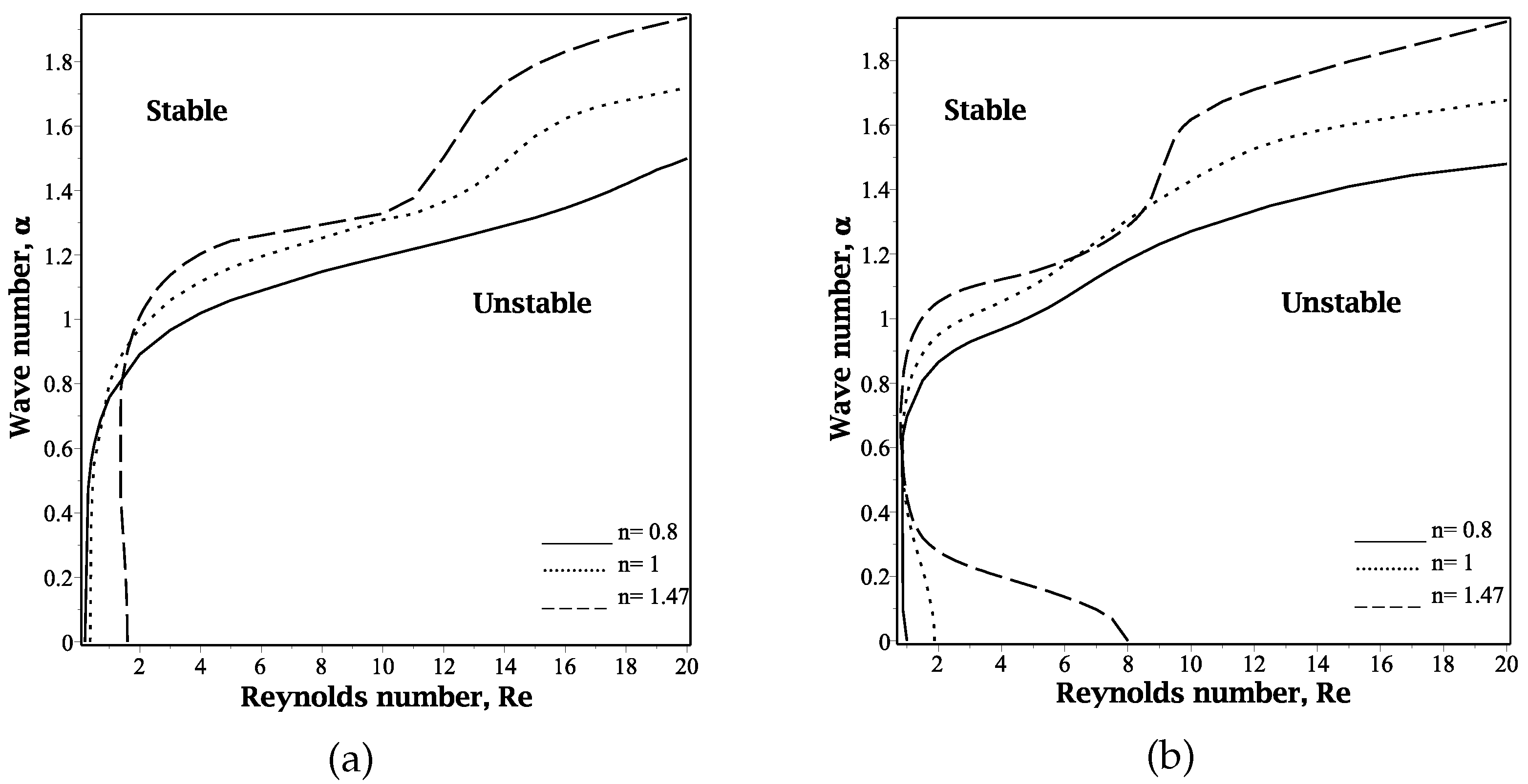
Figure 3 illustrates the effect of varying the power-law index n on the marginal stability curves for $\beta =\pi /2$. This Figure, obtained as a special case by setting $\mathsf{\Gamma }\to \infty$ (the rigid solid layer limit), closely matches with the results from the model developed by Amaouche [26], employing a Galerkin-type approach for the same parameters. Figure 3 shows the marginal stability curves, i.e., the cut-off wave number c versus the Reynolds number, Re. The results shown in Figure 3a are an enlarged view of Figure 3b.

Figure 3a shows that increasing the power-law index n leads to a decrease in the marginal wave number. This implies that, in a low Reynolds number range, shear thickening enhances stability, while shear thinning promotes instability. This effect is clearly established by the fact that effective viscosity is reduced by decreasing n for shear-thinning fluids, whereas it is expected to increase with increasing n for shear-thickening fluids. The result obtained is in good agreement with the conclusions reported in various studies, especially for the case ($\mathsf{\Gamma }\to \infty$) with a rigid plane [26] for power-law fluids. It is clear from Figure 3b that different behavior occurs at high Reynolds numbers, when the destabilizing effects of inertia outweigh the stabilizing influence of gravity. In this case, increasing n increases the range of unstable wave numbers. As we will see later, for moderate and large values of the Reynolds number (Re), the power-law property tries to reduce the most excited disturbance waves by reducing the maximum amplification of perturbation.

Figure 4 presents the marginal stability curve in the (Re, $\alpha$) plane for power-law liquid flow, with variations in the solid deformability parameter $\mathsf{\Gamma }$. Specifically, Figure 4a corresponds to $\mathsf{\Gamma }=10$, while Figure 4b corresponds to $\mathsf{\Gamma }=2$. The Figure shows the presence of different interfacial instability modes. For the general case of gravity-driven flow down a solid substrate ($\mathsf{\Gamma }\to \infty$), the flow becomes unstable to long-wavelength perturbations ($\alpha \ll 1$) when the destabilizing influence of inertia surpasses the stabilizing effect of gravity. Each instability mode has its origin in a jump in mechanical properties at the interfaces, either at the fluid–solid interface or at the fluid–air interface. The Reynolds number along the curve increases as the wave number $\alpha$ increases, with a minimum occurring at $\alpha =0$ (see Figure 3). As demonstrated in previous studies (see, e.g., [6,24,45]) and illustrated in Figure 4, when the substrate’s deformability is sufficiently high ($\mathsf{\Gamma }=10$ and $\mathsf{\Gamma }=2$), the neutral stability curve adopts a profile indicative of the short-wave mode characteristic of the strong viscous regime. In particular, the curve reaches a minimum Reynolds number at a positive value of $\alpha$, indicating that the onset of instability results from the amplification of a finite-length perturbation; from $\mathsf{\Gamma }=10$ to $\mathsf{\Gamma }=2$, this profile becomes more pronounced when the curve adopts a short-wave mode characteristic, reflecting the influence of viscous forces, where instability onset results from the amplification of finite-length perturbations. This instability occurs from the exchange of energy between the fluids and the deformable solid layer through tangential velocities at the interface.

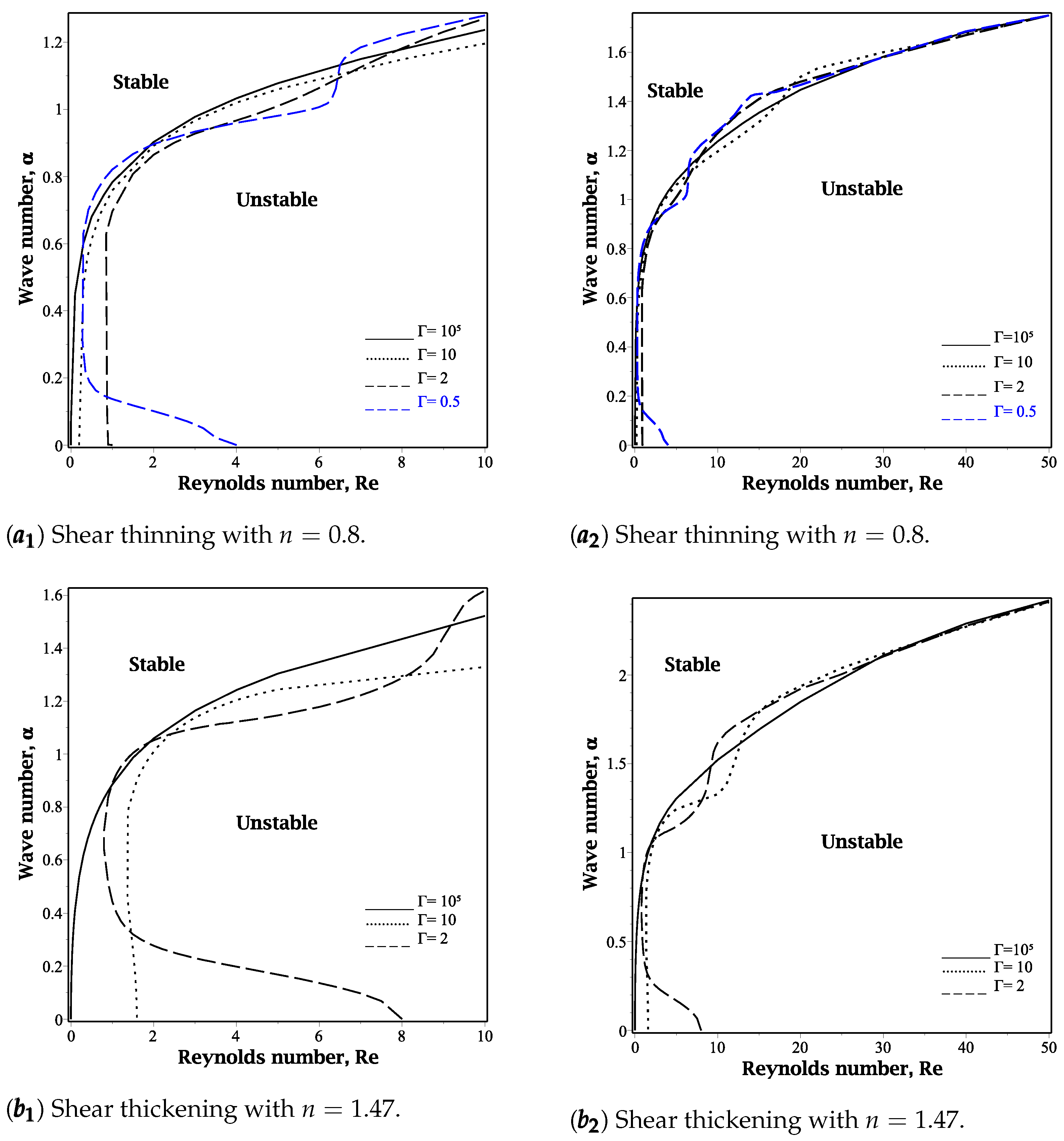
The influence of the deformability parameter $\mathsf{\Gamma }$ on surface and interface instabilities is illustrated in Figure 5. Specifically, panel (a) depicts the case of shear-thinning behavior with $n=0.8$, while panel (b) corresponds to shear-thickening behavior with $n=1.47$. For high Reynolds numbers, no significant deviation from the neutral stability curves is observed when varying the deformability of the solid layer ($\mathsf{\Gamma }$). A similar behavior is noted for Newtonian fluids ($n=1$), though the corresponding curve is not shown. However, at low Reynolds numbers, where inertial effects are negligible, a distinct pattern emerges: for higher values of $\mathsf{\Gamma }$ ($\mathsf{\Gamma }\to \infty$), the Reynolds number (Re) increases monotonically with the wave number $\alpha$. In contrast, for lower values of $\mathsf{\Gamma }$ (ranging from approximately 0.5 to 2), the neutral stability curve exhibits a minimum. This characteristic is observed in both shear-thinning and shear-thickening fluids. It implies that when the solid layer is sufficiently deformable, there exists a minimum Reynolds number beyond which no unstable modes arise. This effect is more pronounced for pseudo-plastic fluids, as illustrated in Figure 5b.

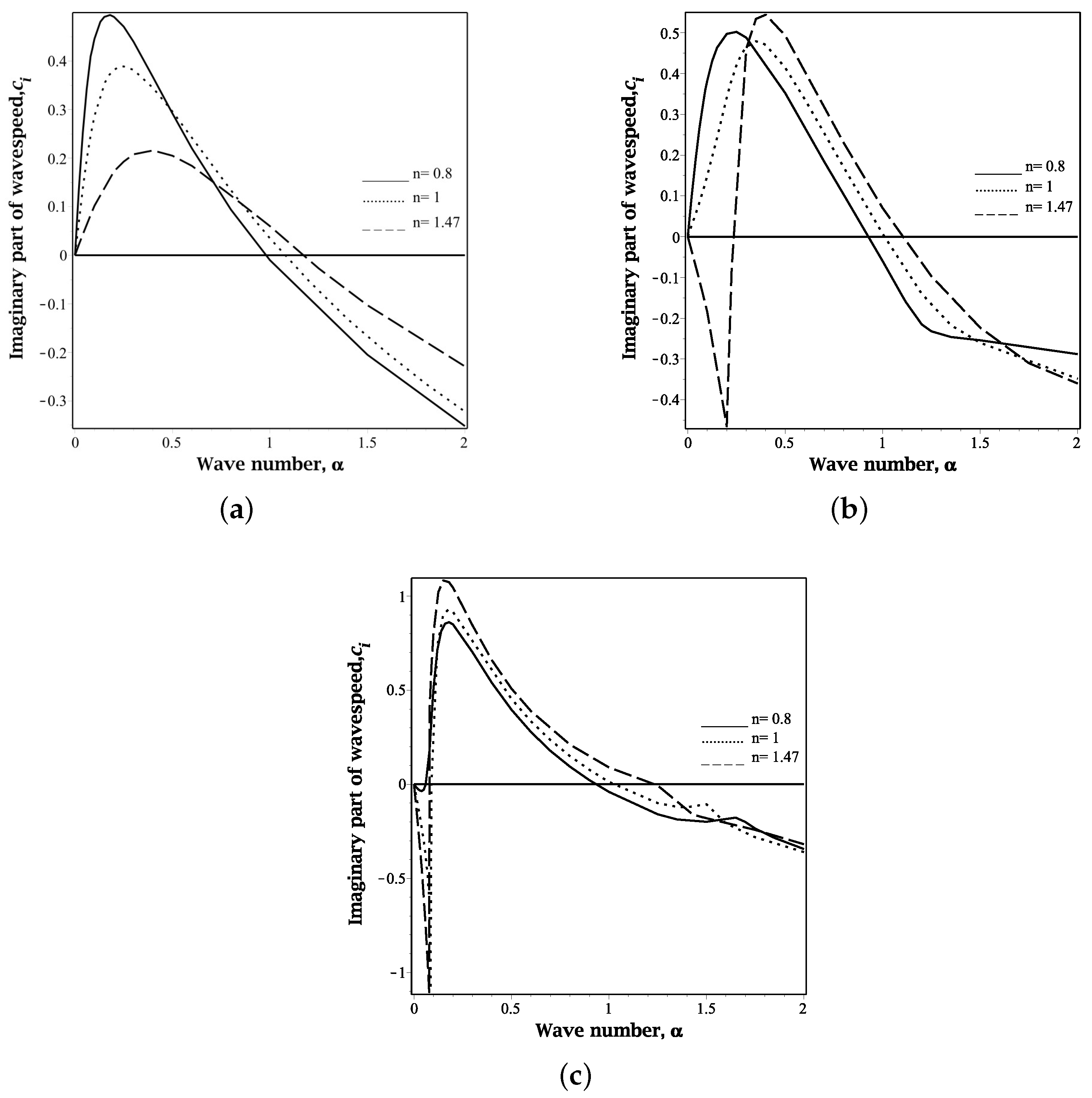
To further investigate both surface and interfacial modes, Figure 6 presents the variation of the complex wave celerity, $c_i$, as a function of $\alpha$ for different values of $\mathsf{\Gamma }$: (a) $\mathsf{\Gamma }\to \infty$, (b) $\mathsf{\Gamma }=2$ and (c) $\mathsf{\Gamma }=0.5$. When the solid layer is non-deformable ($\mathsf{\Gamma }\to \infty$), the flow remains unstable ($c_i>0$) for long-wavelength perturbations, with the dominant mode being a surface mode, as described in [6]. Notably, the complex wave celerity $c_i$ increases as the power-law index n decreases (see Figure 6a for Re = 3). Additionally, the range of unstable wave numbers shrinks as n decreases.

The results align well with previous findings in the literature [26,46]. Figure 6b,c illustrate that as the solid layer becomes more deformable ($\mathsf{\Gamma }=2$ and $\mathsf{\Gamma }=0.5$), the coupling between the liquid and the solid leads to very high instability complex wave celerity. By keeping $\mathsf{\Gamma }=2$ and increasing the power-law index ($n=0.8$, 1, $1.47$), the velocity of the complex wave increases significantly. At $n=1.47$, an unstable interface mode appears and stability ($c_i<0$) is observed within a narrow wave number range ($0<\alpha <0.23$) for the shear-thickening fluid (see Figure 6b). A similar analysis for higher deformability ($\mathsf{\Gamma }=0.5$) with variations of $n=0.8$, 1, and $1.47$ shows that an unstable interfacial mode appears for all values of n that are considered. Moreover, the maximum complex wave celerity also rises with an increasing n value, in contrast to the behavior observed in the non-deformable case, as shown in Figure 6a. Figure 6c shows that as the value of n increases, the wave number spectrum and the complex wave celerity also increase. This confirms that the power-law properties of the fluid favor the development of disturbances when the flow is unstable. It can be seen that n has a significant effect on the fast-growth mode. A comparison of Figure 6a–c indicates that increasing deformability enhances the maximum complex wave celerity of the surface mode, thereby exerting a destabilizing effect. Overall, the findings demonstrate that the instability of the film flow is significantly amplified by the deformability of the solid layer, and increasing this deformability induces finite-wavelength instabilities.

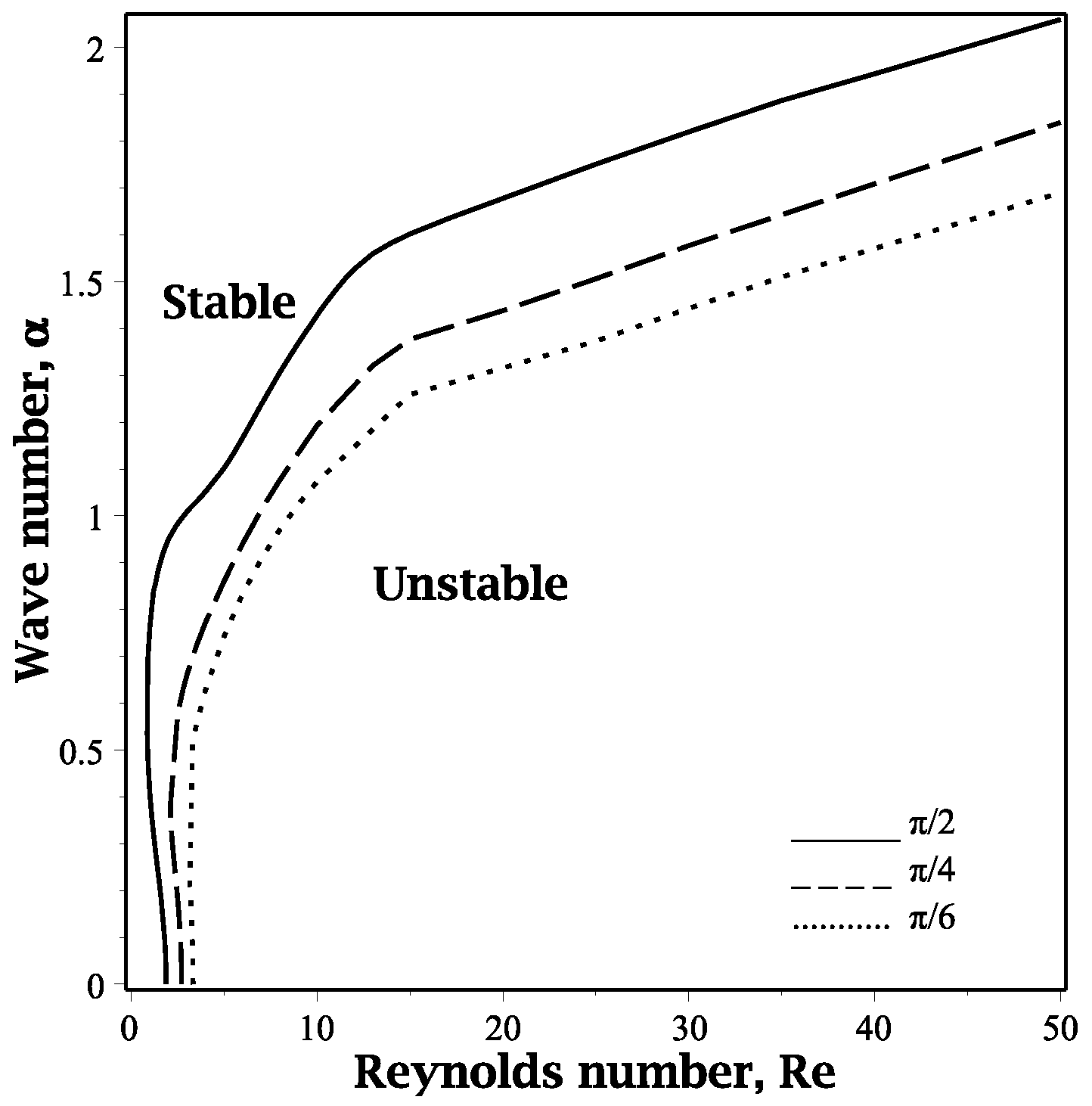
In Figure 7, we focus on the case when $n=1$ and $\mathsf{\Gamma }=2$ and various $\beta$. It can be seen that as $\beta$ increases, instability becomes stronger and the critical Reynolds number decreases. At $\beta =2$ (vertical flame), the flow system shows the highest instability due to the strong influence of gravity and shear flows.

The critical Reynolds number values below which the flow is stable are $1.875$, $2.708$, and $3.318$ for $\beta ={\displaystyle \frac{\pi }{2}}$, $\beta ={\displaystyle \frac{\pi }{4}}$ and $\beta ={\displaystyle \frac{\pi }{6}}$, respectively. The results are in excellent agreement with the results given theoretically by Shankar et al. [24] using the long-wave asymptotic analysis, who found the following expression for the critical Reynolds number:

$${\mathrm{Re}}_c={\displaystyle \frac{5}{6}}cot\beta +{\displaystyle \frac{15}{2}}{\displaystyle \frac{S_0}{\mathsf{\Gamma }}}.$$

To obtain this critical Reynolds number, one must set $c_1=0$, while also noting that our definition of $\mathsf{\Gamma }$ corresponds to $1/\mathsf{\Gamma }$ in Shankar’s formulation, and that $S_0=H$.

Note that for Newtonian liquid flowing down an inclined rigid plane ($\mathsf{\Gamma }\to \infty$), the value of the critical Reynolds number is identical to Yih’s [6] result.

5. Conclusions

We have investigated the stability of a power-law liquid film flow coupled with a neo-Hookean deformable solid layer. A numerical approach based on the Riccati matrix method is used to analyze the effects of solid deformability and power-law properties on interfacial instabilities. By reformulating the Orr–Sommerfeld eigenvalue problem as a nonlinear initial value problem, the Riccati matrix approach eliminates parasitic solutions and effectively addresses the divergence of apparent viscosity at the free surface, which is a common limitation of traditional methods. This work represents the first application of the Riccati matrix approach to the stability analysis of power-law films. Our results show that, for shear-thickening fluids, short-wave instabilities emerge when the rigidity parameter $\mathsf{\Gamma }=2$. On the other hand, for shear-thinning fluids, they appear at $\mathsf{\Gamma }=0.5$. The predicted instability arises from the energy exchange between the fluid and the deformable solid layer via tangential velocities at the interface. In the rigid substrate limit, at low Reynolds numbers, shear thinning enhances instability, while shear thickening is stabilizing. The opposite behavior occurs when inertial effects become significant. When the solid substrate is sufficiently soft, a new instability mode appears even in the Newtonian case, highlighting the crucial role of solid deformations. The power-law index n also significantly affects stability as n increases, with both the wave number spectrum and the growth rate increasing. This confirms that the interplay between fluid rheology and substrate elasticity strongly amplifies instability development.

References

1. Nikravesh, S.; Ryu, D.; Shen, Y.L. Surface Wrinkling versus Global Buckling Instabilities in Thin Film-Substrate Systems under Biaxial Loading: Direct 3D Numerical Simulations. Adv. Theory Simul. 2022, 5, 2200183. [Google Scholar] [CrossRef]
2. Benney, D.J. Long waves on liquid films. J. Math. Phys. 1966, 45, 150–155. [Google Scholar] [CrossRef]
3. Pumir, A.; Manneville, P.; Pomeau, Y. On solitary waves running down an inclined plane. J. Fluid Mech. 1983, 135, 27–50. [Google Scholar] [CrossRef]
4. Benjamin, T.B. Instability of liquid film flows. J. Fluid Mech. 1957, 2, 554–574. [Google Scholar] [CrossRef]
5. Chen, K. Wave formation in the gravity-driven low-Reynolds number flow of two liquid films down an inclined plane. Phys. Fluids A Fluid Dyn. 1993, 5, 3038–3048. [Google Scholar] [CrossRef]
6. Yih, C.-S. On the stability of liquid films. Phys. Fluids 1963, 6, 321–334. [Google Scholar] [CrossRef]
7. Shaqfeh, E.S.G.; Larson, R.G.; Fredrickson, G.H. The stability of gravity-driven viscoelastic film flow at low to moderate Reynolds number. J. Non-Newton. Fluid Mech. 1989, 31, 87. [Google Scholar] [CrossRef]
8. Amatousse, N.; Ait Abderrahmane, H.A.; Mehidi, N. Traveling waves on a falling weakly viscoelastic fluid film. Int. J. Embed. Syst. 2012, 54, 27–41. [Google Scholar] [CrossRef]
9. Pascal, J.-P.; Vacca, A. Instabilities of a shear-thinning fluid falling over an undulating porous layer. J. Non-Newton. Fluid Mech. 2021, 298, 104693. [Google Scholar] [CrossRef]
10. Davis, S.H. Thermocapillary instabilities. Annu. Rev. Fluid Mech. 1987, 19, 403–435. [Google Scholar] [CrossRef]
11. Thiele, U.; Vega, J.M.; Knobloch, E. Long-wave Marangoni instability with vibration. J. Fluid Mech. 2006, 54, 61–93. [Google Scholar] [CrossRef]
12. Chang, H. Wave evolution on a falling film. Annu. Rev. Fluid Mech. 1994, 26, 103–136. [Google Scholar] [CrossRef]
13. Hinch, E.J. A note on the mechanism of the instability at the interface between two shearing fluids. J. Fluid Mech. 1984, 144, 463–465. [Google Scholar] [CrossRef]
14. Amaouche, M.; Mehidi, N.; Amatousse, N. Linear stability of two-layer film flow in an inclined channel: A second-order weighted residual approach. Phys. Fluids 2007, 19, 084106. [Google Scholar] [CrossRef]
15. Weinstein, S.J.; Ruschak, K.J. Coating flows. Annu. Rev. Fluid Mech. 2004, 36, 29–53. [Google Scholar] [CrossRef]
16. Grotberg, J.B.; Jensen, O.E. Biofluid mechanics in flexible tubes. Annu. Rev. Fluid Mech. 2004, 36, 121–147. [Google Scholar] [CrossRef]
17. Berger, S.A.; Jou, L.-D. Flows in stenotic vessels. Annu. Rev. Fluid Mech. 2000, 32, 347–382. [Google Scholar] [CrossRef]
18. Shapiro, A.H.; Jaffrin, M.Y.; Weinberg, S.L. Peristaltic pumping with long wavelengths at low Reynolds number. J. Fluid Mech. 1969, 37, 799–825. [Google Scholar] [CrossRef]
19. He, J.; Hou, Q.; Yang, X.; Duan, H.; Lin, L. Isolated slug traveling in a voided line and impacting at an end orifice. Phys. Fluids 2024, 36, 022101. [Google Scholar] [CrossRef]
20. Zhang, P.; Shao, W.; Arvin, H.; Chen, W.; Wu, W. Nonlinear free vibrations of a nanocomposite micropipes conveying laminar flow subjected to thermal ambient: Employing invariant manifold approach. J. Fluids Struct. 2025, 135, 104311. [Google Scholar] [CrossRef]
21. Xiong, F.; Wang, L.; Huang, J.; Luo, K. A thermodynamically consistent phase-field lattice Boltzmann method for two-phase electrohydrodynamic flows. J. Sci. Comput. 2025, 103, 1–32. [Google Scholar] [CrossRef]
22. Song, Y.; Huang, G.; Yin, J.; Wang, D. Three-dimensional reconstruction of bubble geometry from single-perspective images based on ray tracing algorithm. Meas. Sci. Technol. 2024, 36, 016010. [Google Scholar] [CrossRef]
23. Wu, Y.; Chen, C.; Meng, R.; Chen, Y.; Ba, L.; Liu, Y.; Yi, X. The interfacial polymerization reaction induced by intermolecular dipole–dipole interaction for the preparation of nanofiltration membrane under the low concentration of the aqueous monomers. Sep. Purif. Technol. 2025, 131, 131750. [Google Scholar] [CrossRef]
24. Shankar, V.; Sahu, A.K. Suppression of instability in liquid flow down an inclined plane by a deformable solid layer. Phys. Rev. E 2006, 73, 016301. [Google Scholar] [CrossRef] [PubMed]
25. Jain, A.; Shankar, V. Instability suppression in viscoelastic film flows down an inclined plane lined with a deformable solid layer. Phys. Rev. E 2007, 76, 046314. [Google Scholar] [CrossRef]
26. Amaouche, M.; Djema, A.; Ait Abderrahmane, H. Film flow for power-law fluids: Modeling and linear stability. Eur. J. Mech. B/Fluids 2012, 34, 70–84. [Google Scholar] [CrossRef]
27. Perazzo, C.A.; Gratton, J. Steady and traveling flows of a power-law liquid over an incline. J. Non-Newton. Fluid Mech. 2004, 118, 57–64. [Google Scholar] [CrossRef]
28. Orszag, S.A. Accurate solution of the Orr-Sommerfeld stability equation. J. Fluid Mech. 1971, 50, 689–703. [Google Scholar] [CrossRef]
29. Mamou, M.; Khalid, M. Finite element solution of the Orr-Sommerfeld equation using high precision Hermite elements: Plane Poiseuille flow. Int. J. Numer. Methods Fluids 2004, 44, 721–735. [Google Scholar] [CrossRef]
30. Karan, P.; Chakraborty, J.; Chakraborty, S. Small-scale flow with deformable boundaries. J. Indian Inst. Sci. 2018, 98, 159–183. [Google Scholar] [CrossRef]
31. Yarin, A.L.; Roisman, I.V.; Tropea, C. Collision Phenomena in Liquids and Solids; Cambridge University Press: Cambridge, UK, 2017. [Google Scholar]
32. Noble, P.; Vila, J.-P. Thin power-law film flow down an inclined plane: Consistent shallow-water models and stability under large-scale perturbations. J. Fluid Mech. 2013, 735, 29–60. [Google Scholar] [CrossRef]
33. Gkanis, V.; Kumar, S. Instability of gravity-driven free-surface flow past a deformable elastic solid. Phys. Fluids 2006, 18, 044103. [Google Scholar] [CrossRef]
34. Kumaran, V.; Muralikrishnan, R. Spontaneous growth of fluctuations in the viscous flow of a fluid past a soft interface. Phys. Rev. Lett. 2000, 84, 3310. [Google Scholar] [CrossRef] [PubMed]
35. Tomar, D.S.; Sharma, G. Manipulation and control of instabilities for surfactant-laden liquid film flowing down an inclined plane using a deformable solid layer. Phys. Fluids 2018, 30, 014104. [Google Scholar] [CrossRef]
36. Verma, M.K.S.; Kumaran, V. Stability of the flow in a soft tube deformed due to an applied pressure gradient. Phys. Rev. E 2015, 91, 043001. [Google Scholar] [CrossRef]
37. Malvern, L.E. Introduction to the Mechanics of a Continuous Medium; Prentice-Hall: Englewood Cliffs, NJ, USA, 1969. [Google Scholar]
38. Holzapfel, G.A. Nonlinear Solid Mechanics: A Continuum Approach for Engineering; John Wiley & Sons: Chichester, UK, 2000. [Google Scholar]
39. Gkanis, V.; Kumar, S. Instability of creeping Couette flow past a neo-Hookean solid. Phys. Fluids 2003, 15, 2864–2871. [Google Scholar] [CrossRef]
40. Davey, A. On the numerical solution of difficult eigenvalue problems. J. Comput. Phys. 1977, 24, 331. [Google Scholar] [CrossRef]
41. Miladinova, S.; Lebon, G.; Toshev, E. Thin-film flow of a power-law liquid falling down an inclined plate. J. Non-Newtonian Fluid Mech. 2004, 122, 69–78. [Google Scholar] [CrossRef]
42. Liu, J.; Paul, J.D.; Gollub, J.P. Measurements of the primary instabilities of film flows. J. Fluid Mech. 1993, 250, 69–101. [Google Scholar] [CrossRef]
43. Smith, M.K. The mechanism for the long-wave instability in thin liquid films. J. Fluid Mech. 1990, 217, 469–485. [Google Scholar] [CrossRef]
44. Spodareva, L.A. Stability of non-Newtonian fluid flows. J. Appl. Mech. Tech. Phys. 2000, 41, 446–451. [Google Scholar] [CrossRef]
45. Quéré, D. Fluid coating on a fiber. Annu. Rev. Fluid Mech. 1999, 31, 347–384. [Google Scholar] [CrossRef]
46. Sisoev, G.M.; Dandapat, B.S.; Matveyev, K.S.; Mukhopadhyay, A. Bifurcation analysis of the travelling waves on a falling power-law fluid film. J. Non-Newton. Fluid Mech. 2007, 141, 128–137. [Google Scholar] [CrossRef]
Figure 1. Schematic of the flow configuration for a power-law liquid film falling down an inclined rigid plane covered by an elastic deformable solid layer.
Mathematics 13 01533 g001
Figure 2. A flowchart summarizing the methodology for the linear stability analysis of a power-law liquid film flowing over a deformable inclined plane, covering system definition, formulation, linearization, Riccati transformation, numerical solution, and stability analysis.
Mathematics 13 01533 g002
Figure 3. Neutral stability curves from the numerical solution of the Orr–Sommerfeld equation for the rigid plane limit ( Γ ), compared to those given by Amaouche [26] (diamonds) for n = 1.47 and n = 0.8 . The parameters used are β = π / 2 , W = 1 , σ = 2 , S 0 = 0.5 , and ρ = 1.1 .
Mathematics 13 01533 g003
Figure 4. The variation in the shape of instability curves in the (Re, α ) plane, highlighting the presence of both surface and interface modes for different values of Γ and n. The remaining parameters are set to W = 1 ,   σ = 2 ,   ρ = 1.1 and S 0 = 0.5 . In (a), Γ = 10 , while in (b), Γ = 2 . In panel (b), the dotted and dashed lines correspond to the short-wave mode, whereas the solid line represents the long-wave mode.
Mathematics 13 01533 g004
Figure 5. Neutral stability curves in the (Re, α ) plane for different values of Γ . Panels ( a 1 ) and ( a 2 ) represent the shear-thinning case with n = 0.8 , where ( a 1 ) is an enlarged view of ( a 2 ). Similarly, panels ( b 1 and b 2 ) correspond to the shear-thickening case with n = 1.47 , with ( b 1 ) being an enlarged version of ( b 2 ). The parameter values for W , σ , ρ , S 0 , and β remain the same as in Figure 3 and Figure 4.
Mathematics 13 01533 g005
Figure 6. The variation of the complex wave celerity, c i , as a function of the wave number, α , for Re = 3 and different values of the power-law index. The cases considered are (a) Γ = , (b) Γ = 2 , and (c) Γ = 0.5 . The parameter values for W , σ , ρ and S 0 remain the same as in Figure 3.
Mathematics 13 01533 g006
Figure 7. The variation in the shape of the instability curves in the (Re, α ) plane for varying inclination angles is shown for n = 1 , Γ = 2 and different values of the angle: β = π 6 , β = π 4 , and β = π 2 . The parameter values for W, σ , ρ , and S 0 remain the same as in Figure 3.
Mathematics 13 01533 g007
Disclaimer/Publisher’s Note: The statements, opinions and data contained in all publications are solely those of the individual author(s) and contributor(s) and not of MDPI and/or the editor(s). MDPI and/or the editor(s) disclaim responsibility for any injury to people or property resulting from any ideas, methods, instructions or products referred to in the content.