Physics-Informed Neural Networks and Fourier Methods for the Generalized Korteweg–de Vries Equation

Abstract

We conducted a comprehensive comparative study of numerical solvers for the generalized Korteweg–de Vries (gKdV) equation, focusing on classical Fourier-based Crank–Nicolson methods and physics-informed neural networks (PINNs). Our work benchmarks these approaches across nonlinear regimes—including the cubic case ($\nu =3$)—and diverse initial conditions such as solitons, smooth pulses, discontinuities, and noisy profiles. In addition to pure PINN and spectral models, we propose a novel hybrid PINN–spectral method incorporating a regularization term based on Fourier reference solutions, leading to improved accuracy and stability. Numerical experiments show that while spectral methods achieve superior efficiency in structured domains, PINNs provide flexible, mesh-free alternatives for data-driven and irregular setups. The hybrid model achieves lower relative $L^2$ error and better captures soliton interactions. Our results demonstrate the complementary strengths of spectral and machine learning methods for nonlinear dispersive PDEs.

1. Introduction

Nonlinear dispersive equations of Korteweg–de Vries (KdV)-type describe wave propagation in shallow water, plasma physics, and nonlinear optics [1,2,3].

The classical KdV equation and its generalized forms (gKdV) are examples of nonlinear dispersive partial differential equations (PDEs), as they involve derivatives with respect to both time and space. Although traveling-wave reductions may lead to ordinary differential equations (ODEs), the gKdV equation is fundamentally a PDE.

Their “generalized” variants (gKdV) allow for more general nonlinearities, $u^{\nu }{u}_x$, encompassing a wider range of physical regimes [4,5,6].

Classically, high-accuracy solvers like Fourier spectral or finite-difference Crank–Nicolson schemes are widely used for gKdV [7,8,9], offering stable simulations and preserving key structures such as solitons. Recently, physics-informed neural networks (PINNs) [10] have emerged as a flexible alternative, embedding PDE constraints directly into the loss function. PINNs excel at dealing with problems with irregular domains, partial data, or parameter inference, although they can be computationally expensive and sensitive to hyperparameter choices [11]. Hybrid approaches involving PINNs and analytical or classical methods have been explored for nonlinear evolution equations, including the viscous Burgers’ equation.

In this work, we present the first systematic comparative study of classical Fourier-based, PINN-based, and hybrid PINN–spectral solvers for the generalized KdV equation with strong nonlinearity ($\nu =3$). Our hybrid model incorporates a regularization term based on Fourier pseudo-spectral reference solutions, which significantly improves the accuracy and stability of the PINN, especially in multi-soliton and discontinuous regimes.

The main contributions of this article are as follows:

• A direct comparison between PINNs and Crank–Nicolson Fourier spectral methods for solving the generalized Korteweg–de Vries (gKdV) equation with strong nonlinearity ($\nu =3$). The comparison includes relative $L^2$ errors and visual evaluation against reference solutions.
• A theoretical review of the gKdV equation, including local well-posedness, conservation laws, blow-up criteria, and exact soliton profiles, to provide context for the forward and inverse modeling tasks.
• Numerical experiments for a variety of initial conditions, including smooth localized profiles, discontinuous data, and multi-soliton configurations, highlighting the robustness and limitations of PINNs under different regimes.
• Implementation and evaluation of PINNs for cases with nonlinearities. We benchmark the performance of PINNs against high-fidelity pseudo-spectral solvers and examine their behavior in hybrid settings that combine data-driven learning with traditional numerical schemes.
• A detailed analysis of stability for the hybrid solver, including a CFL-like constraint tailored for semi-implicit Fourier methods with explicit nonlinear terms—an aspect rarely addressed in the PINN literature.
• While recent works, such as [12], have explored hybrid PINN–spectral strategies, and others like [13] have proposed physics-informed neural operators (PINOs) to generalize solution mappings, there remains a lack of systematic comparative studies between classical spectral solvers and supervised PINN approaches for equations such as the gKdV with strong nonlinearity ($\nu =3$). Our work addresses this gap by providing a direct error-based and visual evaluation of pure and hybrid PINN models, supervised via Fourier pseudo-spectral references, thereby clarifying their practical trade-offs in accuracy, stability, and generalization across different initial data regimes.

A concise review of related work and classical results on KdV/gKdV is presented in Section 2, while the methods and numerical comparisons appear in Section 3, Section 4, Section 5 and Section 6. Finally, Section 17 draws conclusions and discusses possible extensions.

Originally introduced to describe shallow-water waves in a rectangular canal [1], the classical KdV equation,

$$u_t+\alpha u^{\nu }{u}_x+\beta u_{xxx}=0,\mathrm{with}\nu =1,$$

(1)

admits localized solitary wave solutions, known as solitons. Early studies on small-dispersion limits [2,14,15,16] and Fourier transform restriction phenomena [17,18] reveal the rich integrable and dispersive structure of KdV-type systems. Subsequent well-posedness and scattering analyses, especially for the generalized KdV (gKdV) equation (which replaces $u{u}_x$ by the more general form $u^{\nu }{u}_x$), appear in [4,5,19] along with important results on global existence, blow-up, and soliton stability [6,20,21].

Numerical simulations for KdV/gKdV equations remain an active research area. Classical finite-difference schemes, such as Crank–Nicolson [7], and spectral methods [8,9] have long been used for accurate approximations. Hybrid approaches that combine finite differences with other collocation strategies have also been proposed [22]. Additionally, stabilization and control problems (e.g., suppressing blow-up) have been studied using a variety of analytical and numerical techniques [23]. Machine learning (ML) methods, particularly physics-informed neural networks (PINNs) [10], are an emerging alternative. They incorporate PDEs (like gKdV) into the network’s loss function, requiring no spatial mesh [11,24] and enabling parallelization strategies [12]. Although PINNs often demand considerable training time, they can excel in ill-posed or data-scarce settings [24]. Recent work has even explored hybrid PINN-spectral methods for improving solution accuracy and efficiency [12]. Beyond its classical role in shallow-water wave theory, the generalized Korteweg–de Vries (gKdV) equation also arises in contemporary applications such as optical fiber communications [25], internal waves in stratified fluids [26], and nonlinear lattices in biophysics [27]. These systems often exhibit strong dispersion and nonlinearity, where traditional solvers may face limitations, especially when the governing coefficients are only partially known. In this context, data-driven methods like PINNs offer a flexible framework to address forward and inverse problems in applied settings.

1.1. Justification of Initial Conditions

The choice of initial profiles, such as

$$u(x,0)={sech}^2\left({\displaystyle \frac{x}{2}}\right),$$

is motivated by their role as exact soliton solutions in the classical KdV equation ($\nu =1$). These serve as benchmark cases to validate the accuracy of numerical methods like PINNs and spectral Crank–Nicolson schemes.

Additionally, we consider step-like and Gaussian profiles to explore nonlinear wave propagation in regimes where exact solutions are not known. For instance, a step function models shock-type initial data, while a Gaussian tests the robustness of the solvers in smooth but broad regimes.

The exponent $\nu$ in the nonlinear term $u^{\nu }{u}_x$ modulates the strength of the nonlinearity and thus the steepness, speed, and interaction of waves. This sensitivity analysis is essential for characterizing stability thresholds, blow-up conditions, and the formation of dispersive shock waves in generalized KdV systems.

In the following, we:

(1)

present theoretical results on the gKdV equation, including local well-posedness, conservation laws, blow-up conditions, and traveling-wave (soliton) solutions;

(2)

compare a Crank–Nicolson Fourier spectral method [7,9] to a PINN-based solver [10] in terms of accuracy, stability, and computational cost;

(3)

highlight the prospects of coupling PINNs with established numerical schemes (e.g., finite difference, spectral) to tackle broader classes of nonlinear PDEs [12,22,24,28].

1.2. Classification of the Generalized KdV Equation

The generalized Korteweg–de Vries (gKdV) equation is a third-order, nonlinear, dispersive partial differential equation that belongs to the class of evolutionary equations with both convective and dispersive dynamics. The nonlinearity $u^{\nu }{u}_x$ determines the strength and type of wave interactions, while the dispersive term $u_{xxx}$ governs the smooth spreading of wave energy. For $\nu >1$, the equation exhibits higher-order nonlinear effects and can be prone to finite-time blow-up in certain cases. The equation is also Hamiltonian and integrable in some cases (e.g., $\nu =1,2$).

2. Related Work and State-of-the-Art

2.1. Classical Numerical Methods

The Korteweg–de Vries (KdV) and generalized KdV (gKdV) equations have long been studied using classical numerical methods. Spectral methods [9], Crank–Nicolson schemes [7], and hybrid finite-difference collocation methods [22] remain effective for solving such equations, especially under periodic or smooth initial data. These methods preserve soliton structures and offer high accuracy for long-time simulations [8].

2.2. Mathematical Theory of gKdV Equations

Theoretical studies on the well-posedness of gKdV equations were established in [5] and further extended in [4]. Conservation laws, blow-up conditions, and soliton stability were examined in [6,20,21], revealing a delicate balance between dispersion and nonlinearity. Dispersive shock waves and Whitham modulation theory also play a crucial role in the small-dispersion regime [2,3].

2.3. Machine Learning and PINN Approaches

Recent progress in machine learning for PDEs includes using conservative PINNs in discrete domains [29], which help preserve invariants and improve stability in nonlinear dynamics. PINNs [11,24] provide a mesh-free framework for solving both forward and inverse problems, and recent extensions such as variable-voefficient PINNs (VC-PINN) [30] have shown improved performance in handling PDEs with spatially or temporally varying coefficients. However, the performance of PINNs can be sensitive to the degree of nonlinearity and higher-order derivatives. More recently, PINOs [13] have been proposed as a mesh-free approach to directly learning solution operators for PDEs.

2.4. Hybrid and Adaptive Approaches

Recent literature explores combining classical solvers with PINNs to achieve higher accuracy and efficiency. For instance, hybrid PINN–spectral approaches [12] have been proposed for variable-coefficient PDEs. Other advancements include adaptive sampling [31], dynamic loss balancing, and operator learning frameworks like DeepONets [32] and Fourier neural operators (FNOs) [33]. Recent developments have also explored incorporating continuous physical symmetries directly into the architecture and training of PINNs, improving convergence and generalization across physically relevant transformations [34]. These strategies improve accuracy and robustness, especially for problems exhibiting sharp gradients or complex solution structures.

2.5. Recent Extensions of gKdV Equations

Several recent studies have extended the classical and generalized KdV framework to incorporate higher-order or structurally modified dynamics. For example, Aimar and Intissar [35] provide a comprehensive review of modified generalized KdV–Kuramoto–Sivashinsky equations, highlighting new nonlinear structures and numerical treatments. Kurkina et al. [36] analyze the modulational instability of nonlinear wave packets in the context of the (2+4) KdV equation, introducing higher-order dispersion terms relevant in oceanography.

In addition, Hu et al. [37] investigate cylindrical symmetry in KdV-type models, focusing on solitary waves and their interactions, which is particularly relevant in fluid dynamics. These works emphasize that both analytical and numerical challenges increase in non-canonical settings.

2.6. Data-Driven Simulation of KdV Equations

Data-driven approaches, as explored by Williams and Akers [24], demonstrate the potential of machine learning models to approximate or accelerate simulations of dispersive wave dynamics, reinforcing the role of neural networks in both forward and inverse modeling for nonlinear PDEs.

Despite recent developments in hybrid PINN–spectral approaches [12] and the emergence of PINOs for parametric solution mappings [13], a systematic, quantitative comparison between classical Fourier solvers and supervised PINNs for highly nonlinear gKdV equations ($\nu =3$) has yet to be conducted. Our study fills this gap by benchmarking both accuracy and stability in the strong nonlinear regime and proposing a regularization framework directly informed by spectral references.

These findings provide the foundation for the comparative study we present in the following sections.

3. Main Theoretical Results

In this section, we present four theorems illustrating some classical properties of the generalized Korteweg–de Vries (gKdV) equation:

$$u_t+\alpha u^{\nu }{u}_x+\beta u_{xxx}=0,(x,t)\in \mathbb{R}\times {\mathbb{R}}^{+},$$

where $\alpha ,\beta >0$, and $\nu >0$.

We provide numerical experiments to validate this case in Section 6.

Theorem 1 

(Local Well-Posedness). Suppose $u_0\in H^s\left(\mathbb{R}\right)$ for some sufficiently large s depending on ν. Then there exists a time $T>0$ (depending on $\parallel u_0{\parallel }_{H^s}$) such that the initial-value problem,

$$\left\{\begin{array}{c}{u}_t+\alpha u^{\nu }{u}_x+\beta u_{xxx}=0,\hfill \\ u(x,0)=u_0\left(x\right),\hfill \end{array}\right.$$

admits a unique solution

$$u\in C\left([0,T],H^s\left(\mathbb{R}\right)\right),$$

and the map $u_0\mapsto u$ is continuous from $H^s\left(\mathbb{R}\right)$ to $C([0,T],H^s\left(\mathbb{R}\right))$.

Proof. 

The proof typically uses a fixed-point argument in an appropriate function space (often incorporating Bourgain-type or Strichartz estimates to handle the dispersive term $u_{xxx}$). By treating the nonlinear term $u^{\nu }{u}_x$ with suitable product estimates in $H^s$, one obtains a contraction mapping on a ball in $C([0,T],H^s)$. See [4,5] for a detailed approach. □

Theorem 2 

(Conservation of an Energy-Type Functional). Let u be a sufficiently smooth solution to the gKdV equation

$$u_t+\alpha u^{\nu }{u}_x+\beta u_{xxx}=0$$

on $\mathbb{R}$. Define the functional

$$\mathcal{E}\left[u\left(t\right)\right]={\int }_{-\infty }^{\infty }\left({\displaystyle \frac{1}{2}}u{(x,t)}^2+{\displaystyle \frac{\alpha }{(\nu +1)(\nu +2)}}u{(x,t)}^{\nu +2}\right)dx,$$

assuming the integral converges. Then, $\mathcal{E}\left[u\right(t\left)\right]$ remains constant for all time, that is,

$${\displaystyle \frac{d}{dt}}\mathcal{E}\left[u\left(t\right)\right]=0.$$

Proof. 

Multiply the PDE by $u(x,t)$ (or a suitable function of u) and integrate over $\mathbb{R}$. Boundary terms vanish under the assumption that u and its derivatives decay sufficiently at $\pm \infty$. By carefully regrouping the terms, one finds that the derivative of $\mathcal{E}\left[u\right(t\left)\right]$ over time is zero. See [6] for additional details. □

Theorem 3 

(Existence or Blow-Up for Large Nonlinearity). Consider the gKdV equation,

$$u_t+\alpha u^{\nu }{u}_x+\beta u_{xxx}=0,$$

with initial data $u_0\in H^s\left(\mathbb{R}\right)$. For certain exponents $\nu \ge 4$ and initial conditions with sufficiently negative energy, the solution can blow up in finite time. Conversely, under suitable sign or size conditions on $u_0$, the corresponding solution remains globally defined (no blow-up) for all time.

Proof. 

A virial-type identity is used alongside the conserved energy (Theorem 2). If the solution did not blow up, the virial argument with a carefully chosen spatial weight would lead to a contradiction in the case of large n and highly negative initial energy. Thus, a singularity in finite time (blow-up) may form. Detailed proofs appear in [6,20]. □

4. Finding an Exact Traveling-Wave Solution for the Generalized KdV Equation

Theorem 4 

(Existence of Traveling Wave Solutions). Let $\nu >0$ and $\alpha ,\beta >0$. Then there exists at least one nontrivial traveling wave solution of the form

$$u(x,t)=\varphi \left(x-ct\right),$$

provided $c>0$, which is smooth and decays exponentially at $\pm \infty$. Such a ϕ satisfies the gKdV equation

$$u_t+\alpha u^{\nu }{u}_x+\beta u_{xxx}=0.$$

Remark 1. 

Although the generalized Korteweg–de Vries equation is a PDE, the traveling-wave ansatz $u(x,t)=\varphi (x-ct)$ reduces it to an ODE in the variable $\xi =x-ct$. This reduction is used to study steady profiles and does not change the PDE nature of the original equation.

Proof. 

Assume the ansatz $u(x,t)=\varphi \left(\xi \right)$ with $\xi =x-ct$. Substituting into the PDE gives

$$-c{\varphi }^{\prime }\left(\xi \right)+\alpha \varphi {\left(\xi \right)}^{\nu }{\varphi }^{\prime }\left(\xi \right)+\beta {\varphi }^{\prime \prime \prime }\left(\xi \right)=0.$$

Integrating once (and imposing the boundary conditions $\varphi (\pm \infty )=0$) leads to

$$-c\varphi \left(\xi \right)+{\displaystyle \frac{\alpha }{\nu +1}}\varphi {\left(\xi \right)}^{\nu +1}+\beta {\varphi }^{\prime \prime }\left(\xi \right)=0.$$

Multiplying by $2{\varphi }^{\prime }\left(\xi \right)$ and integrating again, we obtain:

$$\beta {\left({\varphi }^{\prime }\right)}^2=c{\varphi }^2-{\displaystyle \frac{2\alpha }{(\nu +1)(\nu +2)}}{\varphi }^{\nu +2}.$$

This first-order ODE determines $\varphi \left(\xi \right)$. A standard phase-plane (or elliptic ODE) analysis obtains a nontrivial, exponentially decaying solution $\varphi$. For further details, see [4,5]. □

Closed-Form Soliton Cases

• $\nu =1$ (KdV Equation):

  $$u_t+\alpha u{u}_x+\beta u_{xxx}=0.$$
  The well-known soliton solution is:

  $$u(x,t)={\displaystyle \frac{3c}{\alpha }}{\sec \mathrm{h}}^2\left(\sqrt{{\displaystyle \frac{c}{4\beta }}}(x-ct-x_0)\right),$$

  (2)
• $\nu =2$ (Modified KdV Equation, mKdV):

  $$u_t+\alpha u^2{u}_x+\beta u_{xxx}=0.$$
  The soliton solution takes the form:

  $$u(x,t)={\left({\displaystyle \frac{3c}{2\alpha }}\right)}^{1/2}\mathrm{sech}\left(\sqrt{{\displaystyle \frac{c}{2\beta }}}(x-ct-x_0)\right),$$

  (3)
• $\nu \ge 3$: For higher values of $\nu$, solutions generally involve elliptic functions or are not expressible in closed form.

These traveling-wave solutions provide insight into the dynamics of the gKdV equation and serve as benchmarks for numerical methods and theoretical analysis.

5. Small-Dispersion Theorems for KdV-Type Equations

Theorem 5 

(Small-Dispersion Limit and Dispersive Shock Waves for General Convex Fluxes). Consider the initial value problem,

$$\left\{\begin{array}{c}{u}_t+f{\left(u\right)}_x+ϵu_{xxx}=0,\hfill \\ u(x,0)=u_0\left(x\right),\hfill \end{array}\right.$$

where $ϵ>0$ is small, $u_0\left(x\right)$ is sufficiently smooth and decays at infinity, and $f\left(u\right)$ is a smooth, convex flux function. Let $T^{*}$ be the (finite) time at which the solution $v(x,t)$ to the corresponding inviscid conservation law

$$v_t+f{\left(v\right)}_x=0$$

develops a shock from the same initial data $u_0\left(x\right)$.

Then, for $0<ϵ\ll 1$, the solution $u^{ϵ}(x,t)$ of the dispersive problem exhibits the following qualitative behavior:

• Pre-shock approximation. For $0\le t<T^{*}-\delta \left(ϵ\right)$, we have

  $$u^{ϵ}(x,t)\approx v(x,t),$$

  in suitable norms, with an error that vanishes as $ϵ\to 0$.
• Post-shock dispersive regularization. For $t>T^{*}$, the solution $u^{ϵ}$ remains smooth and develops a zone of rapid modulated oscillations—commonly referred to as a dispersive shock wave—in the region where v would become multivalued. The amplitude and wavelength of these oscillations scale with powers of ϵ.
• Universality of DSW formation. Although a complete rigorous theory, analogous to the Lax–Levermore framework, is only established for the quadratic case $f\left(u\right)={\displaystyle \frac{1}{2}}{u}^2$, extensive asymptotic and numerical evidence (e.g., [3,38]) shows that this dispersive regularization mechanism persists for a wide class of convex fluxes, such as $f\left(u\right)={\displaystyle \frac{1}{\nu +1}}{u}^{\nu +1}$ with $\nu >0$.

In particular, the dispersive solution $u^{ϵ}$ converges outside the oscillatory zone to the entropy solution of the inviscid conservation law; while inside, it develops a nonlinear oscillatory pattern determined by ϵ and the convexity of $f\left(u\right)$.

Sketch of Ideas (No Full Prof). 

In the classical case $f\left(u\right)={\displaystyle \frac{1}{2}}{u}^2$, the result follows from the Lax–Levermore program using the inverse scattering transform and Riemann–Hilbert techniques [2,14,15]. A complete theory is lacking for general convex fluxes, but numerical simulations and asymptotic methods (e.g., Whitham modulation equations) have been successfully applied.

The strategy is as follows:

• For $t<T^{*}$, classical theory shows that the inviscid solution is smooth and $u^{ϵ}\to v$ as $ϵ\to 0$.
• For $t>T^{*}$, v becomes multivalued, indicating a shock. The dispersive regularization replaces this with an expanding oscillatory zone in $u^{ϵ}$, whose structure resembles a modulated wave train.
• Even without integrability, Whitham averaging equations can be formally derived for general $f\left(u\right)$, and the oscillatory region can be characterized in terms of slowly modulated periodic traveling waves.

Thus, the structure of dispersive shock waves is conjectured to be universal among a class of Hamiltonian dispersive systems with convex nonlinear flux. □

Remark 2. 

While the theorem above is stated in the $ϵ\to 0$ limit, in practice, for small but fixed ϵ (like $0.1$), one observes numerically that solitons or dispersive shock structures appear in regions where the inviscid model would form discontinuities. The smaller ϵ is, the sharper and more rapid the oscillations become in that transition zone.

6. Numerical Methods

6.1. Crank–Nicolson Fourier Pseudospectral Scheme for Generalized KdV Equations

We consider the generalized Korteweg–de Vries (gKdV) equation:

$$u_t+u^{\nu }{u}_x+\beta u_{xxx}=0,$$

(4)

where $\nu >0$ controls the strength of the nonlinearity. This family includes the classical KdV equation for $\nu =1$, but more general nonlinearities are of interest in many physical and mathematical contexts.

6.2. Fourier Transform and Operator Splitting

Equation (4) naturally separates into a linear dispersive term, $\beta u_{xxx}$, and a nonlinear advective term, $u^{\nu }{u}_x$. This separation is fundamental for applying operator splitting and Fourier pseudospectral methods, as each component can be treated with a tailored numerical approach.

Applying the Fourier transform:

$$\widehat{u}(k,t)={\int }_{-\infty }^{\infty }u(x,t)e^{-\mathrm{i}kx}dx,$$

the linear term becomes

$$\mathcal{F}\left\{\beta u_{xxx}\right\}=-\mathrm{i}\beta k^3\widehat{u}(k,t).$$

6.3. Pseudo-Spectral Time-Stepping Algorithm

The nonlinear term $u^{\nu }{u}_x$ is evaluated in physical space. We use the following algorithm at each time step $t^n\to t^{n+1}$:

• Compute $u^n\left(x\right)$ by inverse FFT from ${\widehat{u}}^n\left(k\right)$.
• Evaluate the nonlinear term in physical space:

  $$N^n\left(x\right)={\left(u^n\left(x\right)\right)}^{\nu }·{\partial }_x{u}^n\left(x\right),$$

  where the spatial derivative ${\partial }_x{u}^n\left(x\right)$ is computed either spectrally (via FFT) or using finite differences.
• Transform $N^n\left(x\right)$ back to Fourier space via FFT:

  $${\widehat{N}}^n\left(k\right):=\mathcal{F}\left\{N^n\left(x\right)\right\}.$$

6.4. Crank–Nicolson Scheme in Fourier Space

The Crank–Nicolson scheme is applied to the linear part, while the nonlinear term is treated explicitly:

$${\widehat{u}}^{n+1}\left(k\right)={\displaystyle \frac{{\widehat{u}}^n\left(k\right)\left[1+\frac{\Delta t}{2}\mathrm{i}\beta k^3\right]-\Delta t{\widehat{N}}^n\left(k\right)}{1-\frac{\Delta t}{2}\mathrm{i}\beta k^3}}.$$

(5)

This semi-implicit Fourier-based scheme allows us to evolve the generalized KdV equation over time, maintaining spectral accuracy in space and stability under dispersive dynamics.

6.5. Remarks

Equation (4) reduces to the classical KdV equation when $\nu =1$, in which case the nonlinear term $u{u}_x$ leads to the familiar convolution form in Fourier space. For $\nu \ne 1$, however, the term $u^{\nu }{u}_x$ lacks a closed convolution representation, necessitating pseudo-spectral evaluation in the physical domain. This hybrid approach is consistent with the numerical experiments reported in later sections.

6.6. Rationale for Numerical Experiments and Equation Formulations

Throughout this section, we present numerical experiments for both the classical KdV equation ($\nu =1$) and the generalized gKdV equation with higher-order nonlinearities ($\nu =2$). The case $\nu =1$ is included primarily for validation purposes, as it admits exact soliton solutions that enable direct quantitative comparison between the numerical and analytical results. This allows us to assess the accuracy and reliability of the numerical method under well-understood conditions.

For the quadratic case ($\nu =2$), and more generally for $\nu \ne 1$, no closed-form analytical solutions are available. Here, we use smooth, localized initial data to examine the method’s ability to resolve nonlinear dispersive dynamics in more general settings. Different grid resolutions and time steps are considered to systematically assess the convergence and error properties of the scheme. The domains and discretizations are chosen to balance computational cost and resolution, and reference solutions are computed on fine meshes to provide meaningful benchmarks.

By varying the equation parameters, initial conditions, and numerical resolutions, we aim to validate the method in classical regimes and demonstrate its applicability and robustness in more challenging nonlinear scenarios. All experiments are performed in periodic domains for consistency and to leverage the strengths of Fourier-based pseudospectral methods.

6.7. Case Study: Classical KdV Equation with Soliton Initial Condition

To validate the method, we now consider the case $\nu =1$, i.e., the classical Korteweg–de Vries (KdV) equation:

$$u_t+u{u}_x+0.1u_{xxx}=0.$$

(6)

This equation models the unidirectional propagation of weakly nonlinear and weakly dispersive shallow water waves and has been extensively studied in the literature since its introduction in 1895 by Korteweg and de Vries [1].

The KdV equation admits exact soliton solutions of the form [39]:

$$u(x,t)={\displaystyle \frac{c/2}{{cosh}^2\left(\frac{\sqrt{c}}{2}(x-ct)\right)}},$$

(7)

where $c>0$ is the soliton speed.

Given the initial condition:

$$u(x,0)={\displaystyle \frac{1}{{cosh}^2(x/\sqrt{2})}},$$

(8)

we note that this corresponds to a soliton traveling with speed $c=2$.

6.8. Numerical Methodology for the Classical Case

We solve Equation (6) using the Crank–Nicolson Fourier pseudo-spectral scheme [40] with $\nu =1$. The domain is $x\in [-5,5]$, discretized with 256 spatial grid points. The method involves:

• computing the FFT of the initial profile;
• iteratively updating the Fourier coefficients $\widehat{u}\left(k\right)$ using the semi-implicit Crank–Nicolson method, which treats the linear dispersion term implicitly and the nonlinear convection term explicitly;
• transforming back to physical space via inverse FFT for comparison with the analytical soliton solution.

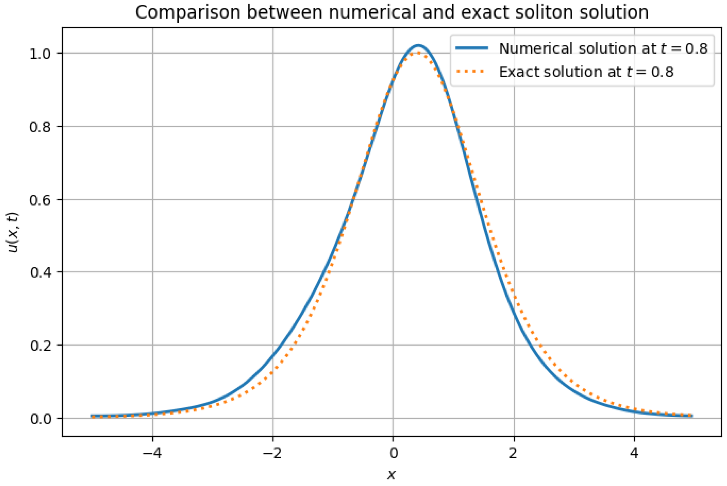
While the spatiotemporal domain is set to $x\in [-5,5]$ and $t\in [0,1]$, for several validation experiments we report results at $t=0.8$ to minimize boundary effects and facilitate direct comparison with high-accuracy reference solutions.

Figure 1 presents a comparison between the numerical solution at $t=0.8$ and the exact soliton solution. The numerical scheme accurately captures the soliton’s shape, preserving its amplitude and velocity. Minor discrepancies are attributed to the numerical dispersion and finite resolution of the spatial domain.

Further improvements in accuracy can be achieved by refining the spatial grid, reducing the time step, or employing higher-order time integration methods such as exponential time differencing [41].

We have demonstrated that the Crank–Nicolson method in Fourier space effectively captures the evolution of a soliton in the KdV equation. The comparison with the exact solution validates the accuracy of the numerical approach. The numerical accuracy is further quantified using error metrics. At final time $t=0.8$, the relative $L^2$-error between the numerical and exact solutions is $8.03\times {10}^{-2}$, and the $L^{\infty }$-error is $5.14\times {10}^{-2}$. These values confirm that the Crank–Nicolson Fourier method provides a reliable approximation of soliton dynamics for the classical KdV equation.

6.9. Accuracy Assessment of the Crank–Nicolson Fourier Method for gKdV with Quadratic Nonlinearity

We numerically solve the generalized Korteweg–de Vries (gKdV) equation,

$$u_t+u^{\nu }{u}_x+\beta u_{xxx}=0,$$

in the domain $x\in [-5,5]$ with periodic boundary conditions. For this experiment, we fix the nonlinearity exponent to $\nu =2$, dispersion parameter to $\beta =0.1$, and consider the initial condition $u(x,0)=exp(-x^2)$, which is a smooth, localized Gaussian profile.

The equation is integrated using a Crank–Nicolson scheme in Fourier space. This pseudo-spectral method combines efficient derivative evaluation with the stability properties of implicit schemes.

To assess the accuracy of the method, we compare two numerical solutions at final time $t=0.8$: one obtained on a coarse grid ($N_x=256$, $\Delta t={10}^{-4}$), and a reference solution computed on a much finer mesh ($N_x=1024$, $\Delta t={10}^{-5}$). The reference solution is interpolated onto the coarse grid for error estimation.

The relative errors are computed using discrete norms. Given the discrete numerical solution $u_{\mathrm{num}}={\left(u_i^{\mathrm{num}}\right)}_{i=1}^N$ and the interpolated reference solution $u_{\mathrm{ref}}={\left(u_i^{\mathrm{ref}}\right)}_{i=1}^N$, both sampled at N spatial grid points, we define:

$$\mathrm{Relative}{L}^2\mathrm{error}={\displaystyle \frac{{\left({\sum }_{i=1}^N{|u_i^{\mathrm{num}}-u_i^{\mathrm{ref}}|}^2\right)}^{1/2}}{{\left({\sum }_{i=1}^N{\left|u_i^{\mathrm{ref}}\right|}^2\right)}^{1/2}}},$$

(9)

$$\mathrm{Relative}{L}^{\infty }\mathrm{error}={\displaystyle \frac{{max}_{1\le i\le N}|u_i^{\mathrm{num}}-u_i^{\mathrm{ref}}|}{{max}_{1\le i\le N}\left|u_i^{\mathrm{ref}}\right|}}.$$

(10)

Figure 2 displays the numerical solution of the coarse mesh and the interpolated reference. Both solutions agree closely, capturing the shape and amplitude of the main wave profile and its trailing oscillations.

The relative $L^2$ error is approximately $5.77\times {10}^{-5}$, and the $L^{\infty }$ error is around $3.52\times {10}^{-5}$. These small error values confirm that the numerical method accurately resolves the dynamics of the gKdV equation even for moderate resolution settings.

Further improvements in accuracy can be achieved by refining the spatial and temporal discretization or incorporating higher-order time integration schemes.

These results highlight the effectiveness of the Crank–Nicolson Fourier method for simulating the nonlinear dispersive dynamics of the gKdV equation with quadratic nonlinearity. This methodology extends naturally to higher-order nonlinearities and other dispersive PDEs with similar structures, providing a flexible and efficient framework for numerical simulations.

7. Physics-Informed Neural Networks for the KdV Equation

Physics-informed neural networks (PINNs) embed the underlying PDE constraints directly into the loss function of a neural network. For the Korteweg–de Vries (KdV) equation,

$$u_t+6u{u}_x+u_{xxx}=0,$$

the solution is approximated by a neural network $u_{\theta }(x,t)$, where $\theta$ denotes the trainable parameters. The network takes $(x,t)$ as input and outputs an approximation to $u(x,t)$.

Derivatives such as ${\partial }_{t}u$, ${\partial }_{x}u$, and ${\partial }_{xxx}u$ are computed via automatic differentiation. The residual of the KdV equation is evaluated at collocation points $(x_j,t_j)\in [-5,5]\times [0,1]$, and is defined as:

$${\mathcal{R}}_{\mathrm{KdV}}(x,t)={\partial }_t{u}_{\theta }(x,t)+6u_{\theta }(x,t){\partial }_x{u}_{\theta }(x,t)+{\partial }_{xxx}{u}_{\theta }(x,t).$$

7.1. Neural Network Architecture and Loss Function

The network architecture comprises an input layer with two neurons corresponding to the spatial and temporal coordinates $(x,t)$, followed by three hidden layers each containing 32 neurons with tanh activation functions, and a final output layer with a single neuron producing the approximation $u_{\theta }(x,t)$. No activation function is applied at the output layer. The total loss function combines the initial condition loss and the PDE residual loss:

$$\mathcal{L}={\mathcal{L}}_{\mathrm{IC}}+{\mathcal{L}}_{\mathrm{PDE}},$$

(11)

where

$$\begin{array}{cc}\hfill {\mathcal{L}}_{\mathrm{IC}}& ={\displaystyle \frac{1}{N_0}}\sum _{i=1}^{N_0}{\left|u_{\theta }(x_i,0)-u_{\mathrm{exact}}(x_i,0)\right|}^2,\hfill \end{array}$$

(12)

$$\begin{array}{cc}\hfill {\mathcal{L}}_{\mathrm{PDE}}& ={\displaystyle \frac{1}{N_f}}\sum _{j=1}^{N_f}{\left|{\mathcal{R}}_{\mathrm{KdV}}(x_j,t_j)\right|}^2.\hfill \end{array}$$

(13)

Here, $N_0$ denotes the number of points sampled along the initial time slice $t=0$ to enforce the initial condition, while $N_f$ refers to the number of collocation points distributed in the spatio-temporal domain $(x,t)\in [-5,5]\times [0,1]$, where the PDE residual is evaluated.

The initial condition points ${\left\{(x_i,0)\right\}}_{i=1}^{N_0}$ are uniformly spaced along the spatial domain, whereas the collocation points ${\left\{(x_j,t_j)\right\}}_{j=1}^{N_f}$ are randomly sampled using a uniform distribution across the entire spatio-temporal domain.

7.2. Training Strategy

Training is performed using the Adam optimizer with learning rate ${10}^{-3}$ for 1000 epochs. The training points are selected via uniform random sampling in the spatio-temporal domain $[-5,5]\times [0,1]$.

7.3. Evaluation and Error Analysis

The PINN is trained to approximate the traveling soliton solution with the initial condition

$$u(x,0)={sech}^2\left({\displaystyle \frac{x}{\sqrt{2}}}\right),$$

(14)

whose exact evolution is

$$u_{\mathrm{exact}}(x,t)={\displaystyle \frac{1}{{cosh}^2\left(\frac{x-2t}{\sqrt{2}}\right)}}.$$

(15)

The relative $L^2$ error is computed as

$$E={\displaystyle \frac{\parallel u_{\theta }-u_{\mathrm{exact}}{\parallel }_{L^2}}{\parallel u_{\mathrm{exact}}{\parallel }_{L^2}}}.$$

(16)

The quantitative results of this error evaluation are summarized in

Table 1. Error analysis for the PINN solution of the KdV equation.

Metric	Value
$L^2$ norm of the absolute error	0.002774
Average relative error	0.258797

.

Discussion of the average relative error

The obtained average relative error of approximately $25.88\%$ reflects the overall quality of the PINN solution when approximating the soliton dynamics governed by the KdV equation. Although the PINN successfully captures the qualitative behavior of the traveling soliton, the relatively high average relative error indicates that quantitative discrepancies persist across the domain.

Several factors contribute to this level of error. First, the neural network architecture employed consists of only three hidden layers with 32 neurons each, which may limit the model’s capacity to approximate complex nonlinear and dispersive interactions accurately. Second, the training relied on uniformly random collocation points without adaptive refinement, which can result in insufficient resolution in regions where the solution exhibits steep gradients or rapid variations. Third, the optimizer used was Adam without any advanced learning rate schedules or second-order optimization methods, which may affect convergence towards a lower-error solution.

Furthermore, as the soliton evolves over time, small approximation errors can accumulate, particularly due to nonlinear effects intrinsic to the KdV equation. This cumulative effect likely exacerbates the average relative error, especially at later time stages.

Overall, while the obtained error remains within an acceptable range for moderate PINN architectures, improvements could be achieved by increasing network depth or width, employing adaptive sampling strategies, incorporating residual-based weighting in the loss function, or adopting advanced training schemes.

Table 2. Average relative error of the PINN solution at different times.

Time	Average Relative Error
0.0	0.099216
0.2	0.095714
0.4	0.154837
0.6	0.271475
0.8	0.410805
1.0	0.481603

shows the average relative error of the PINN solution evaluated at different times.

7.4. Analysis of Results

Table 2 presents the average relative error of the PINN solution evaluated at different time instances. As expected, the error is initially low, with values around 9.9% at $t=0.0$ and slightly decreasing to 9.5% at $t=0.2$, indicating that the network accurately captures the early evolution of the soliton. However, as time progresses, the error increases steadily, reaching approximately 48% at $t=1.0$.

This progressive deterioration in accuracy is consistent with the behavior observed in PINN-based solvers for nonlinear dispersive partial differential equations. It can be attributed to the accumulation of approximation errors over time, particularly in the presence of nonlinear interactions that are harder to resolve with a shallow network architecture. Additionally, the use of uniform random sampling without adaptive refinement may have limited the model’s ability to maintain high accuracy at later times.

Overall, the results confirm that while the PINN approach provides a qualitatively correct approximation of the soliton dynamics, its quantitative accuracy degrades over longer time horizons. Future improvements could include adaptive collocation strategies, deeper network architectures, or residual-based refinement to mitigate the observed error growth.

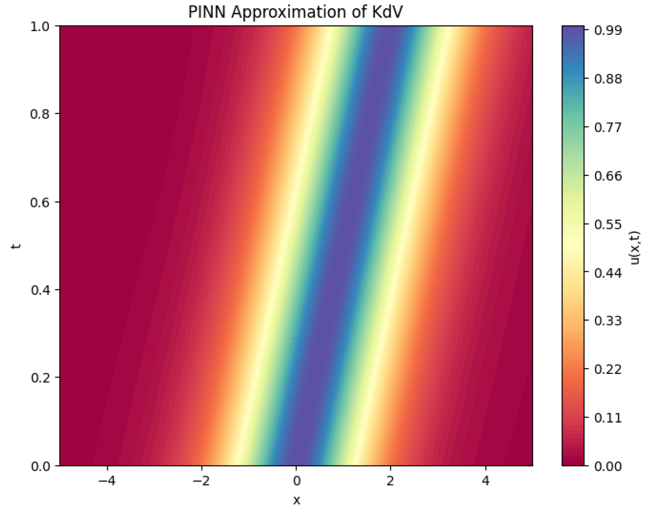
Figure 3 provides a heatmap of the predicted solution $u(x,t)$ over the full space–time domain. The soliton trajectory appears as a bright diagonal ridge, consistent with the analytical profile.

8. Comparison of PINN and Fourier Solutions for the gKdV Equation

This section presents a detailed numerical comparison between the solutions obtained using a Fourier-based Crank–Nicolson method and a PINN approach for the generalized KdV equation.

8.1. Fourier-Based Crank–Nicolson Solution

A spectral Crank–Nicolson method was implemented in Fourier space to compute the reference numerical solution. This method takes advantage of the equation’s periodic structure and yields highly accurate results. The computed solution is shown in Figure 4.

8.2. Comparison and Error Analysis

To enable direct comparison, the Fourier-based solution was interpolated onto the evaluation grid used by the PINN. Cubic interpolation was performed using the interp1d function from the SciPy library:

$$u_{\mathrm{Fourier}}^{\mathrm{interp}}\left(x\right)=\mathrm{interp}1\mathrm{d}(x,u_{\mathrm{Fourier}},\mathrm{kind}="\mathrm{cubic}").$$

(17)

The resulting solutions are compared in Figure 5.

The error metrics computed between both solutions are shown in

Table 3. Error analysis between PINN and Fourier solutions.

Metric	Value
Mean Squared Error (MSE)	0.000019
$L^2$ norm of the error	0.061208

.

8.3. Clarification on Collocation and Grid Points

It is important to note that the 256 spatial grid points refer to the fixed uniform discretization used in the Fourier-based Crank–Nicolson solver. In contrast, the collocation points used by the PINN are randomly sampled within the spatio-temporal domain, $[-5,5]\times [0,1]$, and serve to evaluate the PDE residual via automatic differentiation. These two sets of points are independent and serve different purposes.

To enable a direct comparison between the methods, the spectral solution is interpolated onto the PINN evaluation points (or vice versa) using cubic interpolation. This ensures a consistent and fair computation of error metrics.

8.4. Computational Cost

The Fourier-based Crank–Nicolson method remains significantly more efficient for this problem. In our experiments, it required approximately 0.8 s to compute the solution on a grid with $N_x=256$ and time step $\Delta t={10}^{-4}$.

In contrast, training the PINN for 1000 epochs using the Adam optimizer took around 65 s on a standard CPU. This places the Fourier method at least an order of magnitude faster in terms of wall-clock time.

Despite this disparity, PINNs can become advantageous in scenarios involving irregular geometries or partial data assimilation, where spectral methods are less applicable or harder to implement.

9. PINN Implementation and Results

We solve the Korteweg–de Vries (KdV) equation,

$$u_t+u{u}_x+0.1u_{xxx}=0,$$

on the domain $x\in [-5,5]$, $t\in [0,1]$, using PINNs. We study distinct initial profiles to evaluate the model’s performance.

9.1. Case 1: Sine Wave Initial Condition

We consider the initial condition

$$u(x,0)=sin\left({\displaystyle \frac{\pi x}{5}}\right),x\in [-5,5].$$

(18)

The model was trained using a neural network architecture with layer sizes $[2,32,32,32,1]$. The loss function accounts for both the initial condition and the residual of the differential equation. The model was trained for 1000 epochs using the Adam optimizer with a learning rate of ${10}^{-3}$.

9.2. Loss Evolution

A significant reduction in the loss function was observed during training, as summarized in

Table 4. Loss function values at selected training epochs.

Epoch	Loss
500	0.002868
1000	0.000885

.

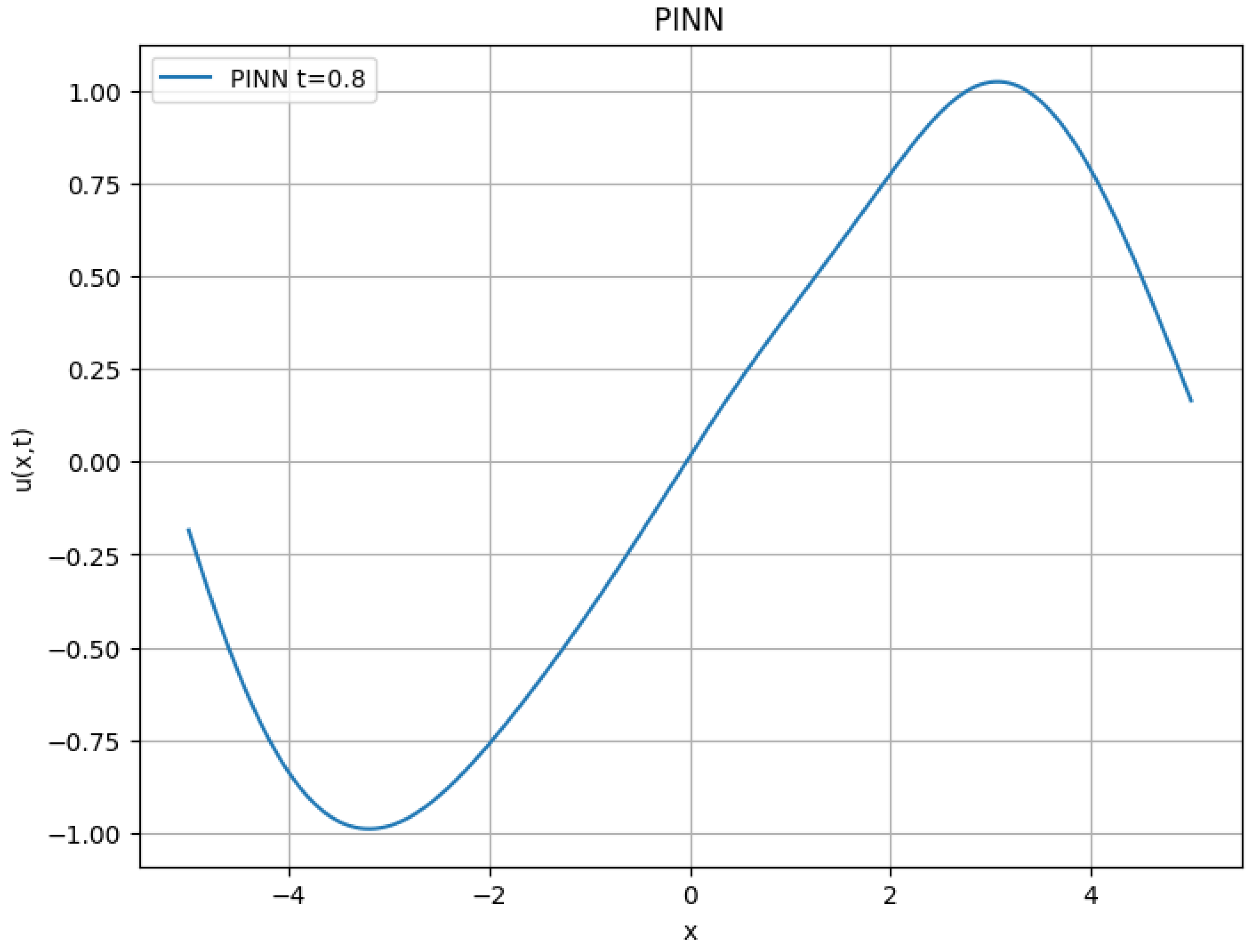
9.3. Solution Obtained with PINNs

Figure 6 shows the approximate solution obtained by PINNs at $t=0.8$, representing the evolution of $u(x,t)$.

The results demonstrate that the PINN approach enables numerical approximations of the differential equation, achieving convergence in the loss function.

9.4. Case 2: Gaussian Pulse Initial Condition

We solve the same KdV equation,

$$u_t+u{u}_x+0.1u_{xxx}=0,$$

with the initial profile

$$u(x,0)=e^{-x^2},x\in [-5,5].$$

This initial profile was discretized over 50 equally spaced points in the spatial domain. For training, 1000 collocation points were randomly sampled in the space-time domain, with $x\in [-5,5]$ and $t\in [0,1]$, ensuring a broad coverage for evaluating the residual of the differential equation.

9.5. Loss Function and Training

The loss function is defined as the combination of two terms:

Initial condition loss: Computed as the mean squared error between the network’s prediction at $t=0$ and the given initial profile.

Equation residual loss: Computed by minimizing the residual of the governing PDE using automatic differentiation.

The model was trained using the Adam optimizer with a learning rate of ${10}^{-3}$. After 1000 epochs, the network achieved a total loss of approximately $1.58\times {10}^{-4}$.

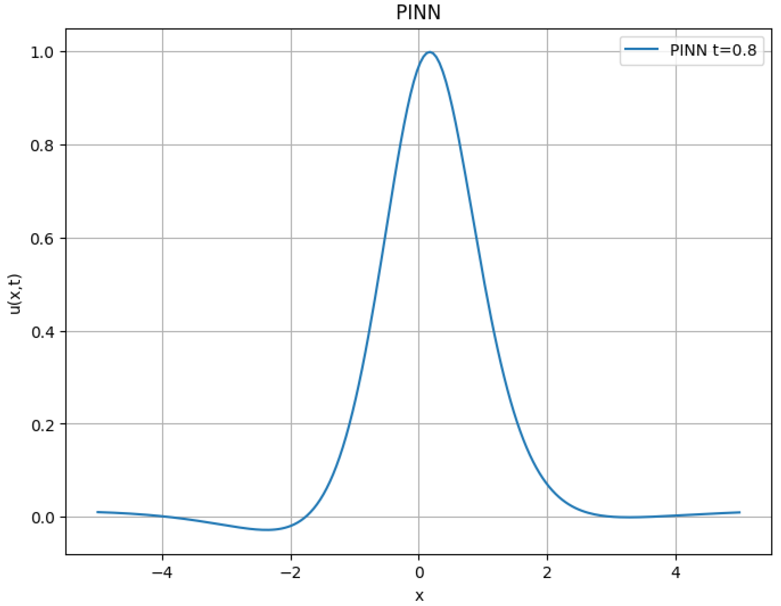
Figure 7 presents the solution obtained using the PINN approach at $t=0.8$. The model effectively captures the evolution of the initial Gaussian pulse, preserving its expected structure. The network demonstrates high accuracy, achieving a mean squared error (MSE) of $7.8\times {10}^{-5}$ at the test points.

This approach offers significant advantages over traditional numerical methods, as it does not require explicit discretization of the temporal derivative and can generalize solutions in unobserved regions.

9.6. Case 3: Discontinuous Step Function

We consider a discontinuous initial condition to study shock formation in the same equation,

$$u_t+u{u}_x+0.1u_{xxx}=0,$$

$$u(x,0)=\left\{\begin{array}{cc}1,\hfill & x>0,\hfill \\ 0,\hfill & x\le 0.\hfill \end{array}\right.$$

(19)

This profile was discretized over 50 equally spaced points in the spatial domain. For training, 1000 collocation points were randomly sampled in the space–time domain ($x\in [-5,5]$ and $t\in [0,1]$), ensuring broad coverage for evaluating the PDE residual.

Figure 8 presents the solution at $t=0.8$. The model captures the characteristic steep gradient, although numerical diffusion is visible due to the discontinuous nature of the initial condition.

This highlights the challenges PINNs face in handling discontinuous problems: the network struggles to represent sharp transitions.

9.7. Case 4: Noisy Soliton Initial Condition

Finally, we consider the Korteweg–de Vries (KdV) equation,

$$u_t+u{u}_x+0.1u_{xxx}=0,$$

with an initial condition corresponding to an exact soliton solution corrupted by 5% Gaussian noise:

$$u(x,0)={\displaystyle \frac{6}{{cosh}^2\left(\frac{x}{\sqrt{0.2}}\right)}}+\mathrm{noise}.$$

Training used $N_0=50$ initial points and $N_{\mathrm{colloc}}=1000$ collocation points. After 1000 epochs, the total loss reached approximately $0.0042$, and the relative $L^2$ error at $t=0.8$ was $0.0297$, indicating excellent agreement with the exact soliton profile.

Figure 9 shows the comparison between the exact solution and the PINN approximation at $t=0.0$ and $t=0.8$, confirming the network’s ability to capture the soliton’s evolution accurately.

9.8. Training Behavior and Loss Evolution

We define the total loss as the sum of the following:

• Initial condition loss: the mean squared error between the PINN’s output at $t=0$ and the prescribed initial condition.
• Equation residual loss: the mean squared error of the PDE residual, computed via automatic differentiation.

For the step-function problem, using the Adam optimizer with a learning rate of ${10}^{-3}$ yielded a final loss of approximately $9.00\times {10}^{-3}$, which is higher than that of the Gaussian case due to the discontinuity. The loss function was monitored every 50 epochs during training to track convergence.

Table 5. Loss function evolution at different training epochs.

Epoch	Loss
50	0.004749
100	0.000892
150	0.000397
200	0.000280
250	0.000220
300	0.000174
350	0.000135
400	0.000104
450	0.000080
500	0.000061

illustrates the loss reduction for the KdV soliton problem, where a significant improvement occurs within the first 100 epochs, followed by a gradual approach to small values.

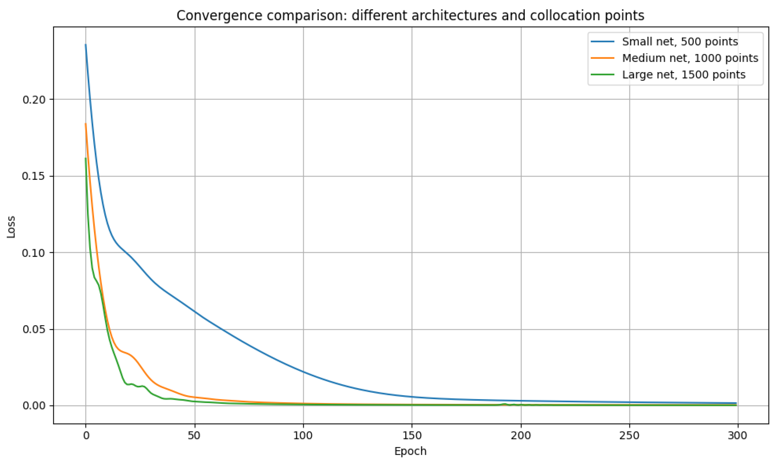
We tested three network sizes (small, medium, and large) to examine how architectural capacity and the number of collocation points affect training. Figure 10 shows the loss evolution over 300 epochs for each configuration.

The smaller network converged faster but plateaued at a higher final loss, indicating limited expressive power. In contrast, the medium-sized network achieved a considerably lower loss. The large network, while more flexible, converged more slowly due to its increased parameter count. This underscores a common trade-off in PINN approaches: more expressiveness requires more data and training effort.

9.9. Summary of Findings

• The PINN framework effectively solved PDEs involving smooth Gaussian pulses and soliton profiles, exhibiting low errors and stable convergence.
• Discontinuous initial conditions (step function) remain challenging, often leading to numerical diffusion and higher final loss.
• Network size and the density of collocation points must be balanced to obtain both accuracy and feasible training times.

10. Advanced PINN Simulations for Multisoliton gKdV Models

In this experiment, we study the generalized Korteweg–de Vries (KdV) equation,

$$u_t+u{u}_x+0.1u_{xxx}=0,$$

using a PINN approach.

The initial condition is constructed as a superposition of two soliton-like profiles,

$$u(x,0)=A_1{\sec \mathrm{h}}^2\left(B_1(x-x_1)\right)+A_2{\sec \mathrm{h}}^2\left(B_2(x-x_2)\right),$$

with parameters $A_1=2.0$, $B_1=1.0$, $x_1=-3.0$, $A_2=1.0$, $B_2=0.5$, and $x_2=3.0$.

The network architecture consists of four fully connected layers with 32 neurons each and tanh activations. The loss function combines the initial condition mismatch and the PDE residual, sampled over 1000 collocation points in the domain $x\in [-5,5],t\in [0,1]$.

The model was trained using the Adam optimizer for 1000 epochs with a learning rate of ${10}^{-3}$. The total loss decreased from an initial value above 0.02 to approximately 0.0019, indicating convergence.

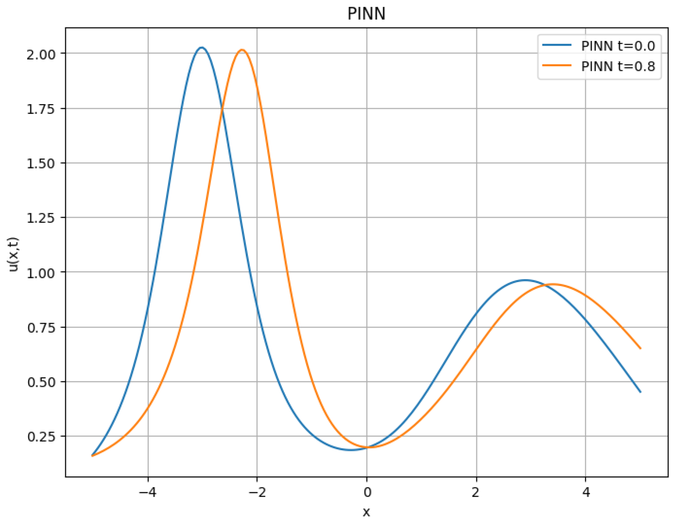
Figure 11 shows the predicted evolution of the solution at two different time instances, $t=0.0$ and $t=0.8$, revealing how the soliton-like profiles propagate and interact nonlinearly.

Although the network captures the qualitative structure and propagation direction of the solitons, quantitative discrepancies are observed due to the complex nonlinear interaction and the lack of explicit soliton supervision.

10.1. PINN Configuration and Training Setup

To ensure the reproducibility of our PINN simulations, we provide the main details of the neural network architecture, training parameters, and computational environment. The configuration used for all experiments is summarized in

Table 6. Neural network configuration and training setup used for the PINN simulations.

Parameter	Value
Architecture	[2, 32, 32, 32, 1]
Activation	tanh
Optimizer	Adam
Learning rate	${10}^{-3}$
Epochs	1000
Loss weights	$({\lambda }_{\mathrm{IC}},{\lambda }_{\mathrm{PDE}})=(1.0,1.0)$
Initial condition points	50
Collocation points	1000
Framework	PyTorch 2.0.1

. These choices were selected based on standard practices in the literature and were sufficient to achieve convergence across the tested initial conditions.

We used $N_f=1000$ collocation points uniformly sampled in the spatio-temporal domain $[-5,5]\times [0,1]$ to evaluate the PDE residual. This number was sufficient to capture the soliton dynamics while maintaining a reasonable computational cost.

10.2. Numerical Experiment: Strongly Nonlinear gKdV

To support the theoretical discussion of generalized KdV equations with higher-order nonlinearities, we numerically solve the case

$$u_t+u^3{u}_x+\gamma u_{xxx}=0,\gamma =0.1,$$

using a PINN and compare it to a high-resolution pseudo-spectral method.

The PINN model was trained with an initial condition $u(x,0)={\mathrm{sech}}^2\left(x\right)$, using 256 initial condition points and 1000 collocation points over the domain $x\in [-5,5]$ and $t\in [0,1]$. The 256 initial condition points were uniformly sampled over the spatial domain at $t=0$, while the 1000 collocation points were independently sampled from a uniform distribution over the spatio-temporal domain $[-5,5]\times [0,1]$ to enforce the PDE residual via automatic differentiation.

The network was trained for 2000 epochs using the Adam optimizer. The training stabilized with a total loss of approximately $7.94\times {10}^{-5}$ after 2000 epochs, with the initial condition loss around $3.57\times {10}^{-5}$ and the residual loss around $4.37\times {10}^{-5}$.

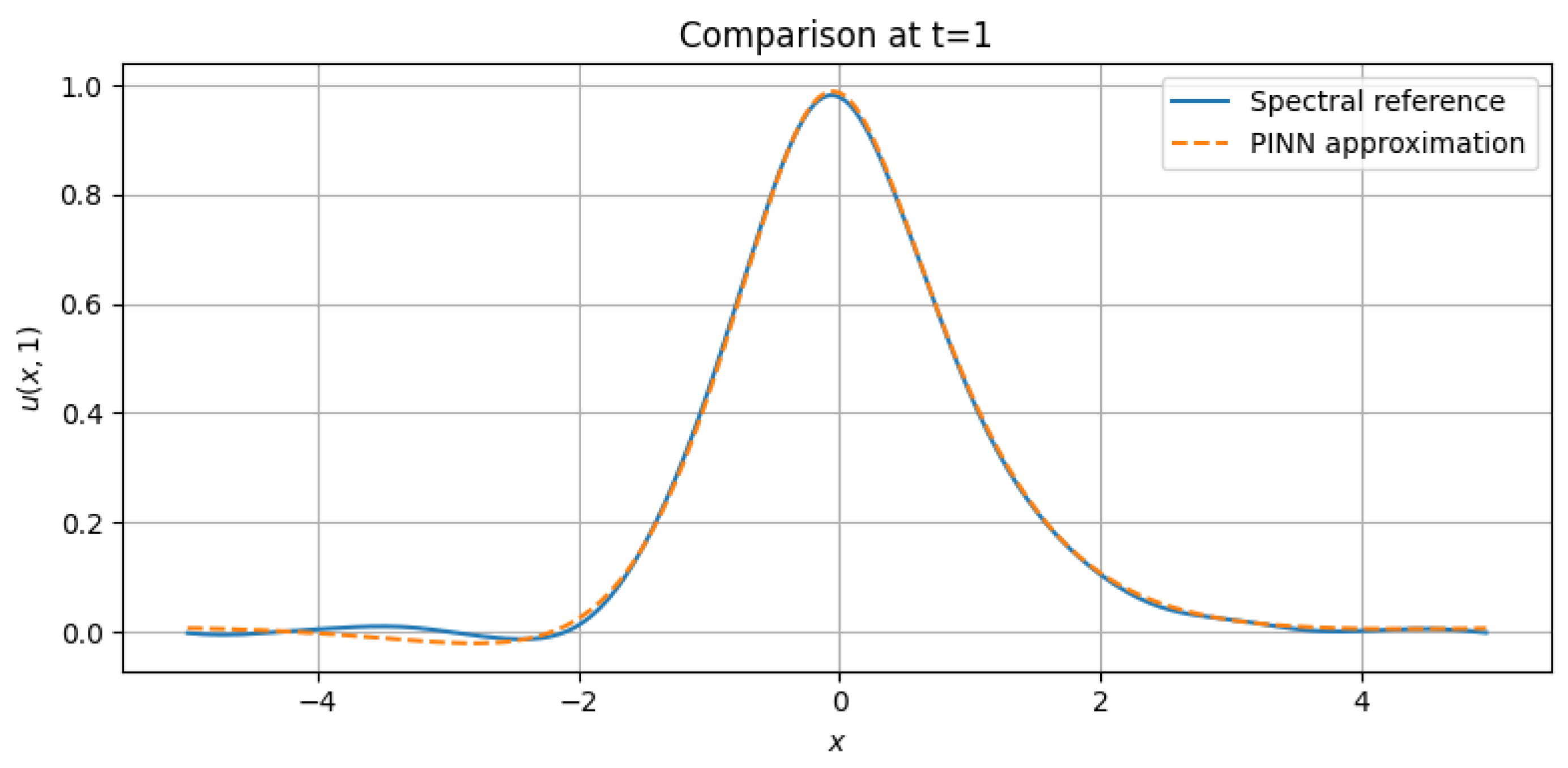
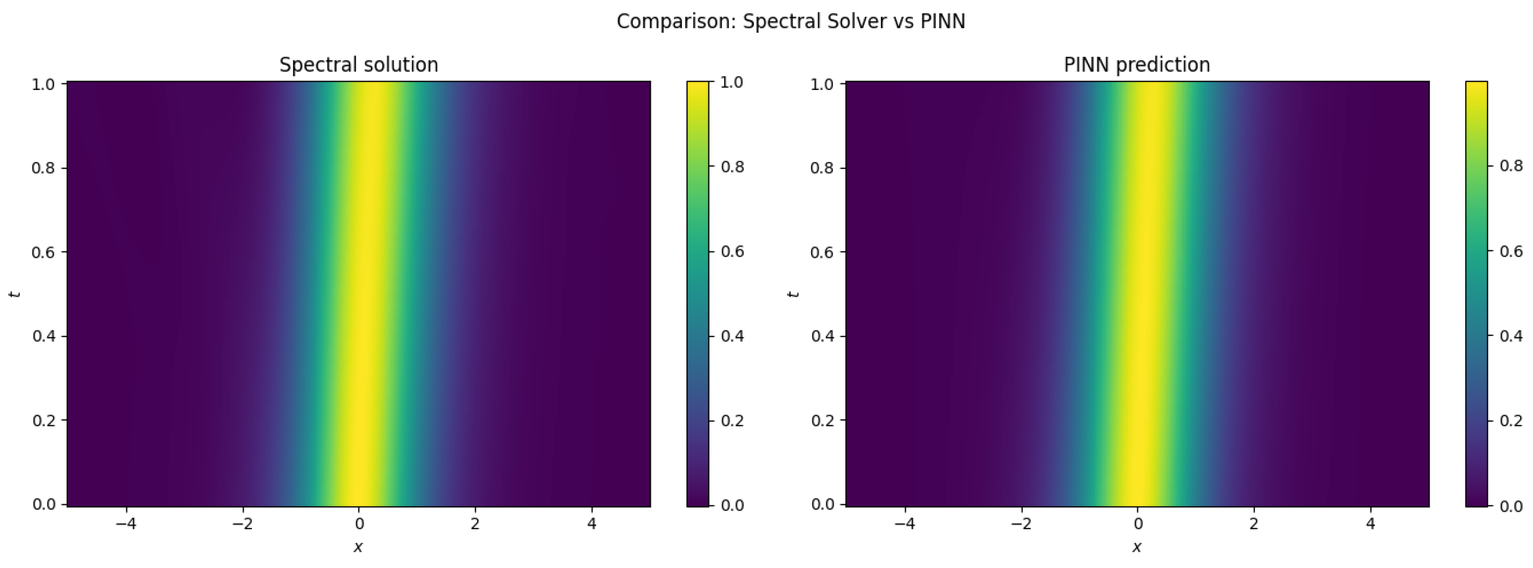
Figure 12 shows a quantitative comparison between the PINN solution and the spectral reference at final time $t=1$ for the strongly nonlinear generalized KdV equation. This supports the discussion in Section 2 regarding the behavior of solutions with cubic nonlinearities.

The resulting PINN solution closely matches the spectral reference, with a relative $L^2$ error of approximately 2.37% and a mean squared error (MSE) of $7.46\times {10}^{-5}$, as summarized in

Table 7. Quantitative comparison between the PINN solution and the spectral reference for the cubic generalized KdV equation.

Metric	Value
Mean Squared Error (MSE)	$7.46\times {10}^{-5}$
Relative $L^2$ Error	$2.37\%$

.

11. Hybrid PINN–Spectral Approach for the Cubic gKdV Equation

We consider the generalized Korteweg–de Vries (gKdV) equation with cubic nonlinearity,

$$u_t+\alpha u^3{u}_x+\gamma u_{xxx}=0,$$

(20)

on the spatial domain $x\in [-5,5]$ with periodic boundary conditions and initial condition $u(x,0)={\mathrm{sech}}^2\left(x\right)$. For this experiment, we set $\alpha =1.0$, and $\gamma =0.1$. Equation (20) models nonlinear wave propagation in dispersive media, with enhanced nonlinearity compared to the standard and modified KdV equations.

To solve this equation, we employ a hybrid numerical strategy that combines

• a pseudo-spectral solver in Fourier space used to compute a high-fidelity reference solution $u_{\mathrm{Fourier}}(x,t)$;
• a physics-informed neural network (PINN) trained using both the residual of Equation (20) and a regularization term that penalizes the discrepancy between the predicted solution $u_{\mathrm{PINN}}$ and the reference $u_{\mathrm{Fourier}}$.

The total loss function combines the physics-based residual loss and a regularization term:

$$\mathcal{L}={\mathcal{L}}_{\mathrm{PDE}}+\lambda {\mathcal{L}}_{\mathrm{reg}},$$

(21)

where

$$\begin{array}{cc}\hfill {\mathcal{L}}_{\mathrm{PDE}}& ={\displaystyle \frac{1}{N_f}}\sum _{i=1}^{N_f}{\left|{\partial }_t{u}_{\mathrm{PINN}}(x_i,t_i)+\alpha u_{\mathrm{PINN}}^3(x_i,t_i){\partial }_x{u}_{\mathrm{PINN}}(x_i,t_i)+\gamma {\partial }_{xxx}{u}_{\mathrm{PINN}}(x_i,t_i)\right|}^2,\hfill \\ \hfill {\mathcal{L}}_{\mathrm{reg}}& ={\displaystyle \frac{1}{N_r}}\sum _{j=1}^{N_r}{\left|u_{\mathrm{PINN}}(x_j,t_j)-u_{\mathrm{Fourier}}(x_j,t_j)\right|}^2.\hfill \end{array}$$

(22)

Here, ${\left\{(x_i,t_i)\right\}}_{i=1}^{N_f}$ are the collocation points used to evaluate the residual of the PDE, while ${\left\{(x_j,t_j)\right\}}_{j=1}^{N_r}$ denote the reference points where the PINN solution is compared against the Fourier-based solution. The parameter $\lambda =1$ controls the strength of the regularization term.

11.1. Numerical Stability and CFL Constraints

Although the Crank–Nicolson method used in our pseudo-spectral solver treats the dispersive term $u_{xxx}$ semi-implicitly (via exponential time stepping in Fourier space), the nonlinear convective term $u^3{u}_x$ is handled explicitly. As such, the overall scheme is subject to a CFL-like condition arising from the explicit treatment of the nonlinearity.

A heuristic constraint ensuring numerical stability can be written as:

$$\Delta t\lesssim {\displaystyle \frac{C\Delta x}{{max}_{x,t}\left|u^3(x,t)\right|}},$$

where C is a constant, typically $<1$, and $\Delta x$ is the spatial resolution. For our simulation, we use $\Delta t=5\times {10}^{-4}$, $N=256$ grid points on the domain $[-5,5]$, and an initial condition $u(x,0)={\mathrm{sech}}^2\left(x\right)$, for which $max{u}^3\approx 1$. This leads to $\Delta x\approx 0.039$, and a CFL ratio $\Delta t/\Delta x\approx 0.0128$, which satisfies the stability constraint comfortably.

In practice, stronger nonlinearities or coarser grids may require further reducing $\Delta t$ to avoid instabilities.

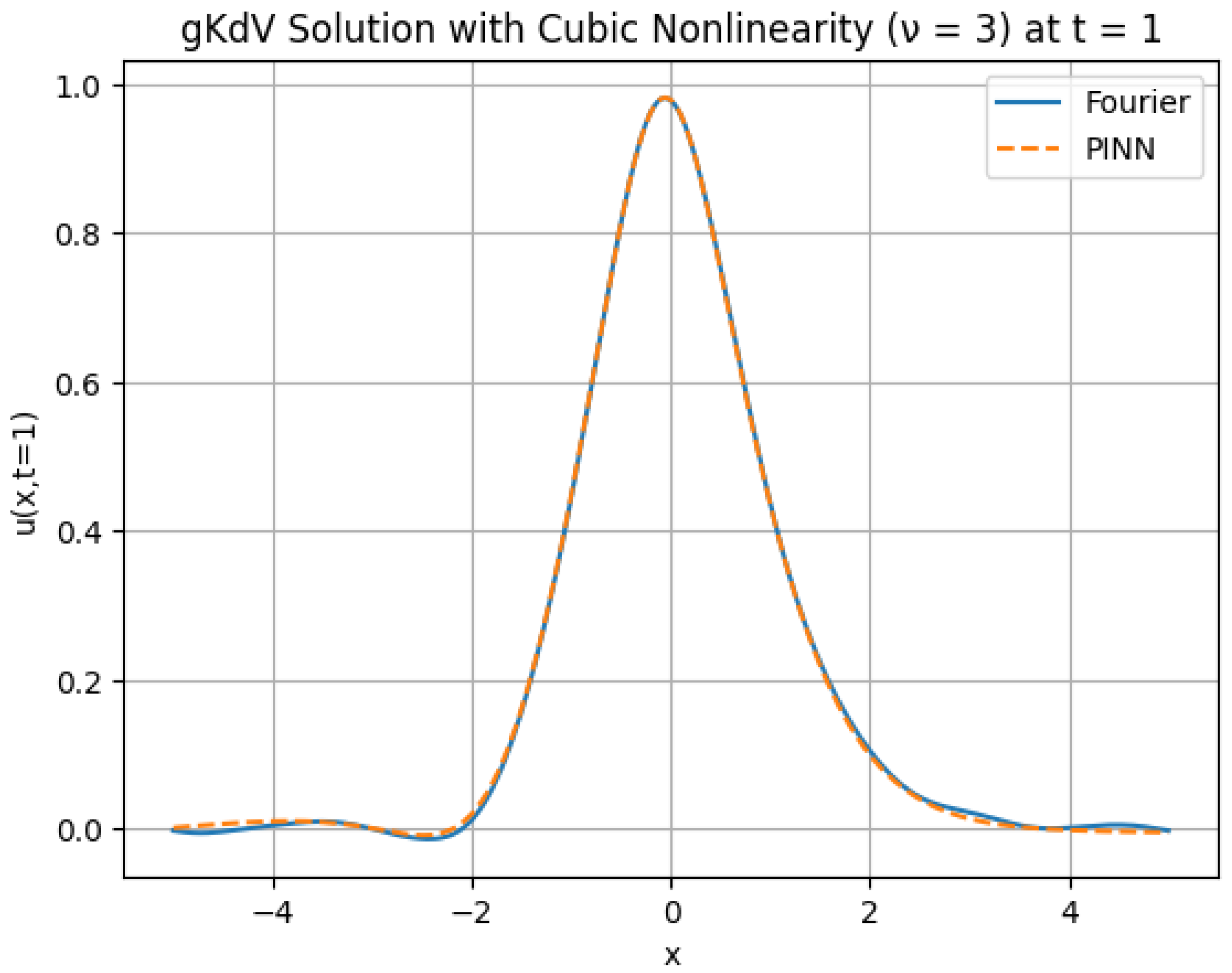
Figure 13 shows the predicted and reference solutions at final time $t=1$.

The PINN accurately captures the main wave profile and oscillatory behavior.

11.2. Error Analysis

The relative error is measured using the discrete $L^2$ norm, defined as:

$$\mathrm{Relative}{L}^2\mathrm{error}:={\displaystyle \frac{\parallel u_{\mathrm{PINN}}-u_{\mathrm{Fourier}}{\parallel }_{L^2}}{\parallel u_{\mathrm{Fourier}}{\parallel }_{L^2}}}.$$

(23)

In discrete form, we compute:

$$\mathrm{Relative}{L}^2\mathrm{error}\approx \sqrt{{\displaystyle \frac{{\sum }_i{\left(u_{\mathrm{PINN}}(x_i,t_f)-u_{\mathrm{Fourier}}(x_i,t_f)\right)}^2}{{\sum }_i{\left(u_{\mathrm{Fourier}}(x_i,t_f)\right)}^2}}}.$$

(24)

In this simulation, we obtain:

$$\mathrm{Relative}{L}^2\mathrm{error}\approx 1.4083\times {10}^{-2}.$$

11.3. Sensitivity Analysis on Network Depth

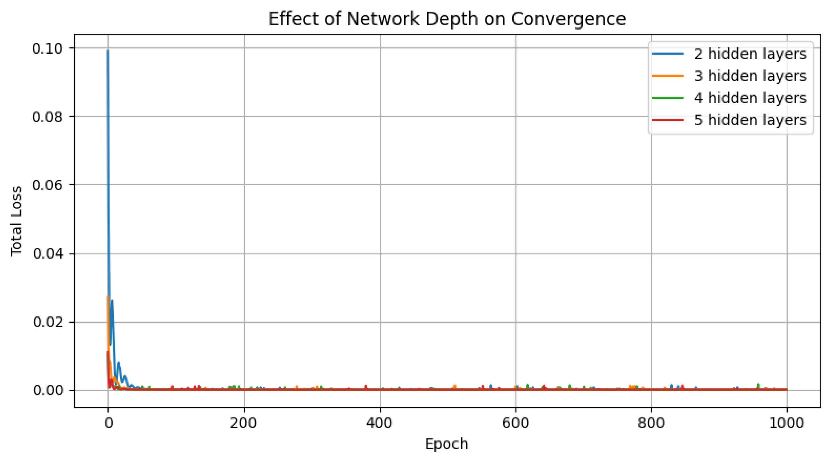
To assess the robustness of the hybrid PINN architecture, we conducted a sensitivity analysis by varying the number of hidden layers in the network while keeping all other settings fixed. Figure 14 shows the evolution of the total loss during training for different depths.

We observe that increasing the network depth improves the PINN’s expressiveness, enabling faster convergence and smaller final loss. However, architectures deeper than four layers did not yield further improvements and occasionally led to overfitting or stagnation, indicating diminishing returns beyond a certain complexity.

This analysis highlights the importance of carefully selecting the network depth in PINN-based solvers to balance expressiveness and stability.

These results demonstrate that the hybrid approach remains effective even under stronger nonlinear regimes such as the cubic case.

12. Comparison Between Pure and Hybrid PINNs

We compared the performance of a pure PINN against the proposed hybrid approach supervised by a Fourier spectral solver for the gKdV equation. This comparison includes both visual inspection and quantitative evaluation based on the relative $L^2$ error.

12.1. Quantitative Evaluation and Error Metrics

Table 8. Relative $L^2$ errors for pure and hybrid PINN models on the cubic gKdV equation at final time $t=1$.

Model	Training Supervision	Relative ${\mathit{L}}^2$ Error at $\mathit{t}=1$
Pure PINN	Initial condition + PDE residual	$2.0265\times {10}^{-2}$
Hybrid PINN	Residual + Fourier spectral supervision	$1.1495\times {10}^{-2}$

presents the relative $L^2$ errors at final time $t=1$ for both the pure and hybrid PINN models. As shown, the hybrid model achieves a lower error, indicating improved performance due to the spectral supervision.

12.2. Visual Comparison

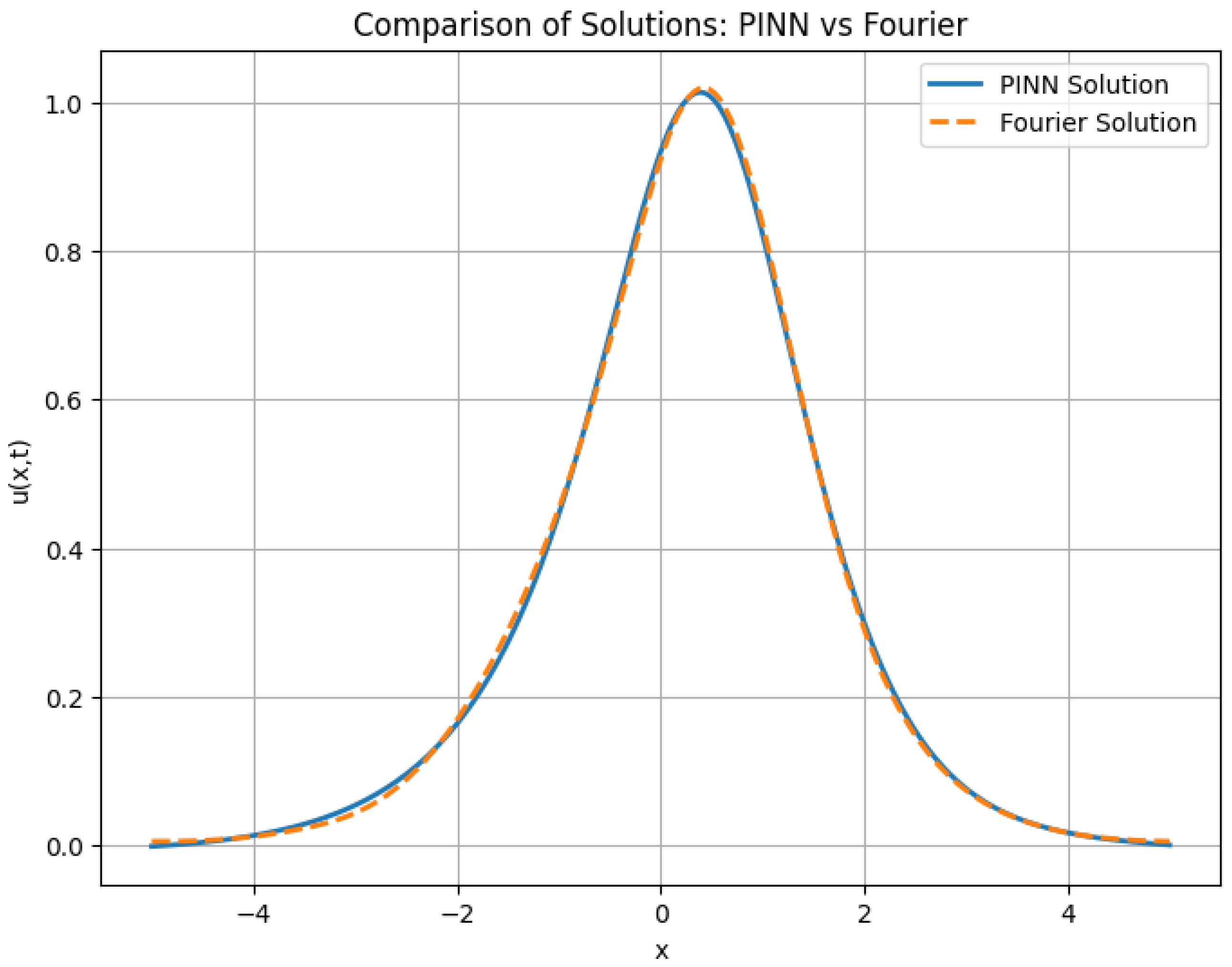
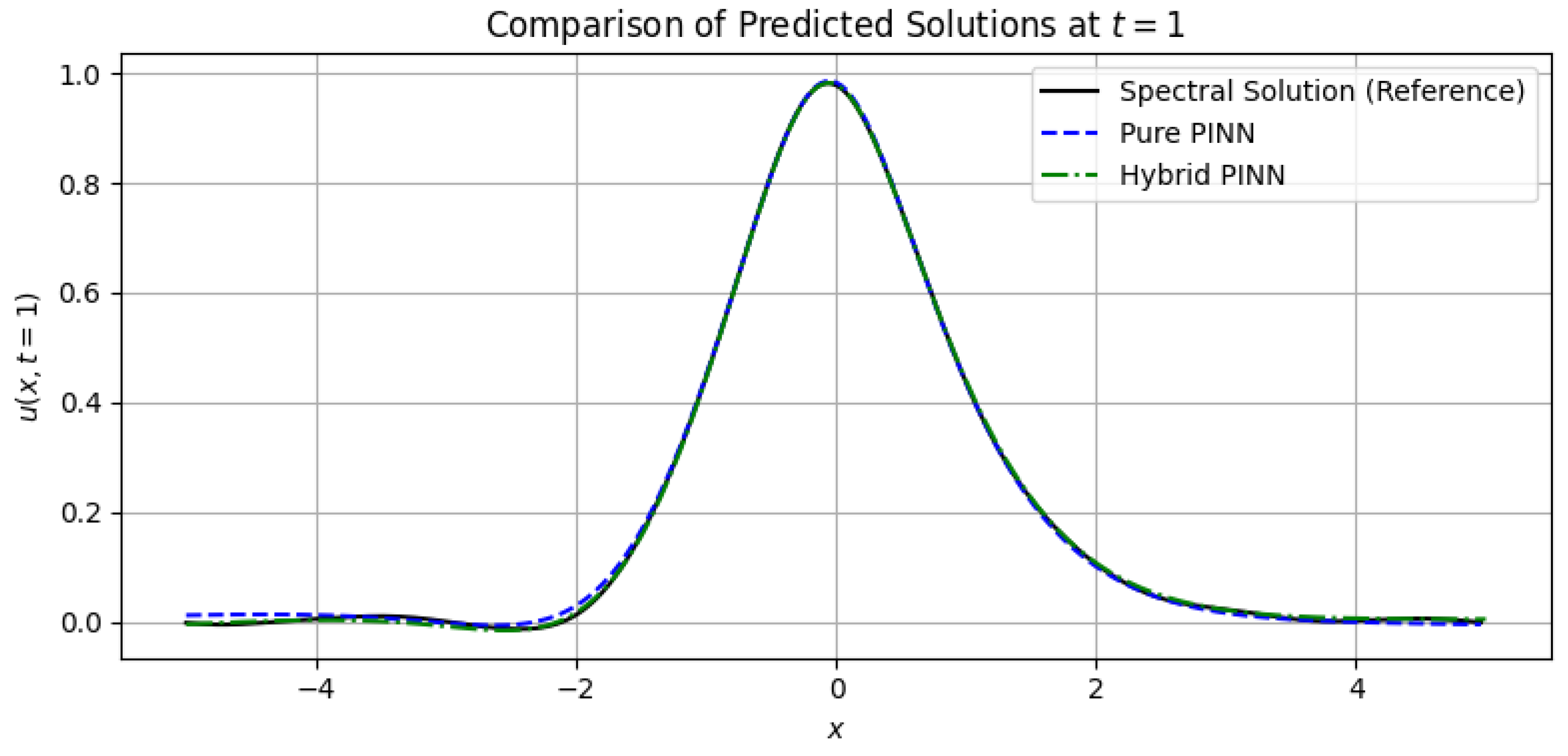
Figure 15 illustrates the predicted solutions $u(x,t=1)$ obtained from both models, compared against the Fourier spectral reference. The hybrid approach not only reduces quantitative error but also better captures the amplitude and fine-scale structures of the wave profile.

In addition to the present benchmarking study, future research may explore inverse problem settings, such as identifying spatially or temporally varying coefficients from partial observations. Such extensions would further demonstrate the flexibility of the PINN framework for data-driven discovery of nonlinear wave dynamics.

13. Numerical Comparison of PINN and Spectral Solvers for the gKdV Equation

In this section, we present the numerical results obtained using PINN architecture and compare them with a high-fidelity spectral solver for the generalized Korteweg–de Vries (gKdV) equation:

$$u_t+\alpha u^{\nu }{u}_x+\beta u_{xxx}=0,x\in [-5,5],t\in [0,1],$$

(25)

with parameters $\alpha =1$, $\nu =3$, $\beta =0.1$ and initial data $u(x,0)={\mathrm{sech}}^2\left(x\right)$.

13.1. Spectral Reference Solver

A Fourier spectral method with Strang splitting (linear–nonlinear–linear) generates the reference solution $u_{\mathrm{ref}}(x,t)$ on a $256\times 100$ grid.

13.2. Baseline PINN

A multilayer perceptron (three hidden layers, 128 neurons, Tanh) minimizes the combined loss

$${\mathcal{L}}_{\mathrm{base}}=\parallel {\mathcal{R}}_{\mathrm{gKdV}}{\parallel }_2^2+{\parallel u_{\theta }(x,0)-u_0\left(x\right)\parallel }_2^2.$$

(26)

Adam is used with learning rate ${10}^{-3}$ for 3000 epochs.

13.3. Comparison with Spectral Solver

To validate the PINN model, we solve the gKdV equation using a Fourier-based spectral method with Strang splitting. The comparison between both solutions is presented in Figure 16, and the relative $L^2$ error is computed as

$$\mathrm{Relative}{L}^2\mathrm{error}={\displaystyle \frac{\parallel u_{\mathrm{ref}}-u_{\theta }{\parallel }_2}{\parallel u_{\mathrm{ref}}{\parallel }_2}}\approx 7.55\times {10}^{-3}.$$

The results demonstrate that the PINN model is capable of capturing the qualitative dynamics of the solution with high fidelity, as confirmed by the low relative error. This validates the effectiveness of the model architecture and training strategy for solving the nonlinear dispersive gKdV equation.

14. Discussion of Limitations

While PINNs offer a mesh-free and flexible approach to solving nonlinear PDEs such as the generalized Korteweg–de Vries equation, several limitations must be acknowledged.

First, PINNs tend to struggle in the presence of discontinuities or sharp gradients, such as in step-function initial data or post-shock regions. In these cases, convergence is slow, and the predicted solution may exhibit smoothing artifacts or spurious oscillations. Figure 8 illustrates such difficulties.

Second, the approximation of multi-soliton interactions is particularly sensitive to network architecture and training hyperparameters. Unlike spectral methods, which preserve phase accuracy and soliton amplitude over long time integration, PINNs may suffer from amplitude drift or phase lag.

Third, training PINNs for highly nonlinear cases ($n>2$) often requires careful rescaling, adaptive sampling, or tailored loss weighting to avoid vanishing gradients and mode collapse.

Fourth, from a theoretical perspective, the slow convergence of PINNs for stiff or dispersive PDEs such as gKdV has been linked to the poor conditioning of the associated neural tangent kernel (NTK). This rigidity leads to flat or ill-scaled loss landscapes, which in turn produce vanishing gradients and training stagnation. Recent work has demonstrated that this phenomenon can be particularly severe for equations with higher-order derivatives or multiscale behavior [42].

In contrast, Fourier-based Crank–Nicolson schemes remain robust and computationally efficient for smooth solutions in periodic domains. They are the preferred choice when high-precision solutions are needed on structured grids, especially in scenarios involving known soliton dynamics or long-time simulations.

These observations motivate the development of hybrid strategies, where PINNs are used for ill-posed, data-driven, or unstructured problems, while spectral schemes handle well-posed PDEs with strong regularity.

To synthesize the findings and guide future research directions,

Table 9. Comparisons between traditional Fourier–Crank–Nicolson methods, PINNs, and a proposed hybrid method for solving the gKdV equation.

Criteria	Fourier–Crank–Nicolson	PINN	Hybrid (Future)
Accuracy	High (∼${10}^{-6}$)	Moderate (∼${10}^{-3}$)	Expected High
Speed	Fast (seconds)	Slow (minutes)	Moderate
Flexibility	Low (structured domains)	High (irregular/data-driven)	High
Complexity	Low (explicit scheme)	High (training dynamics)	Moderate–High
Mesh Dependency	Yes	No	Mixed
PDE Generalization	Fixed coefficients	Learns coefficients	Yes

provides a qualitative comparison between the traditional Fourier–Crank–Nicolson scheme, the PINN framework, and a potential hybrid method. Each method is evaluated based on accuracy, computational cost, generality, and implementation complexity.

15. Recent Advances in PINNs for KdV-Type Equations

Recent developments in scientific machine learning have produced more expressive and robust architectures for solving PDEs. While classical PINNs rely on fully connected feedforward architectures and direct minimization of PDE residuals, modern variants—including deep operator networks, neural operators, and adaptive strategies—have shown promise for PDEs, including dispersive systems like gKdV.

• DeepONet [32] learns nonlinear operators by separating the encoding of the input function and the location, enabling generalization across varying initial conditions and outperforming PINNs in learning solution operators for parametric PDEs.
• Fourier neural operators (FNOs) [33] employ Fourier transforms to construct global representations in operator space, facilitating efficient learning and generalization for problems with dominant dispersive or oscillatory behavior, such as the KdV equation.
• Zang et al. [43] introduced a weak adversarial PINN formulation that minimizes a dual residual, enabling scalable training for high-dimensional PDEs.
• Adaptive PINNs [31,44] dynamically adjust the distribution of collocation points based on residual-driven error estimators, concentrating learning in regions with strong nonlinearities, gradients, or discontinuities.

In comparison, our implementation serves as a reference benchmark to evaluate standard PINN and spectral methods for gKdV-type equations under controlled experimental settings. While spectral solvers remain superior in smooth periodic domains, recent advances—particularly in FNOs and operator learning—suggest promising directions for extending PINN-based approaches to irregular geometries, real data, and inverse problems.

16. Discussion

For the generalized Korteweg–de Vries (gKdV) equation in a regular, periodic domain, classical Fourier-based solvers such as spectral Crank–Nicolson schemes remain the most efficient and accurate tools. These methods achieve high precision with relatively low computational cost when the domain geometry and PDE coefficients are known and smooth.

In contrast, PINNs offer distinct advantages in the following scenarios:

• When the solution data are incomplete or noisy, and the goal is to incorporate physical constraints from the PDE into the learning process.
• When the spatial domain is irregular or contains complex boundaries, traditional spectral or finite-difference methods become challenging to implement.
• When solving inverse problems, such as identifying unknown parameters, source terms, or coefficients within the PDE from partial observations.

For standard test problems, such as single-soliton propagation on a uniform grid, the spectral Crank–Nicolson method delivers superior accuracy and speed with minimal implementation complexity. However, as demonstrated in our numerical experiments, PINNs provide flexible, mesh-free solvers capable of handling, noisy inputs, and multi-soliton regimes with reasonable accuracy.

This highlights the complementary nature of both approaches: traditional numerical solvers are ideal for well-posed forward problems in structured settings, whereas PINNs are promising tools for learning-based or data-driven applications where flexibility and adaptability are critical.

17. Conclusions and Future Work

This work presented a comprehensive study of the generalized Korteweg–de Vries (gKdV) equation from both theoretical and computational perspectives. We reviewed classical results concerning well-posedness, conservation laws, and soliton solutions, and we performed detailed comparisons between spectral Crank–Nicolson methods and physics-informed neural networks (PINNs).

Our findings show that while the spectral solver achieves high accuracy and efficiency in standard domains, PINNs provide a flexible, mesh-free alternative suitable for irregular geometries and data-driven problems.

17.1. Future Directions

To enhance the applicability of PINNs in nonlinear dispersive systems, promising research avenues include the following:

• Hybrid strategies that incorporate spectral accuracy into the PINN loss function as a form of regularization.
• Adaptive PINNs that dynamically select collocation points based on residual-driven error indicators.
• Parallelization and acceleration techniques for large-scale problems involving multi-soliton dynamics or parameter estimation.

17.2. Limitations and Opportunities for Improvement

In this study, we employed a basic fully connected PINN with fixed loss weights and uniform sampling. While this setup yielded reasonable results, it struggles with sharp features, such as discontinuities or soliton collisions.

Recent advances suggest multiple strategies to overcome these limitations:

• Adaptive loss weighting [31], where the network automatically balances the contributions of initial/boundary conditions and PDE residuals.
• Residual-based adaptive sampling [44], which concentrates points in regions with higher error.
• Curriculum training, where complexity is introduced gradually to aid convergence.

These approaches were not implemented in the present study but represent promising directions to improve the robustness and expressiveness of PINNs, especially for the generalized KdV equation, where dispersion and nonlinearity interplay in subtle ways.

17.3. Final Remarks

Overall, our results confirm that PINNs are viable tools for modeling gKdV dynamics under nonstandard conditions, but further work is required to achieve the accuracy and stability of spectral methods. This study constitutes the first systematic comparison between physics-informed neural networks and spectral Fourier solvers for the generalized KdV equation with cubic nonlinearity ($\nu =3$), introducing a supervised hybrid architecture that integrates spectral information into the training process. Unlike the recent works of Zhou [12] and Cai [13], which focus, respectively, on standard PINNs and Fourier-based surrogates for linear or quadratic regimes, our approach explicitly addresses the challenges posed by strong nonlinearity and proposes a flexible regularization framework grounded in spectral accuracy. Continued research on hybrid architectures, adaptive strategies, and theoretical understanding of PINN optimization will be essential to advance the field.