Abstract
In high-dimensional data analysis, main effects and interaction effects often coexist, especially when complex nonlinear relationships are present. Effective variable selection is crucial for avoiding the curse of dimensionality and enhancing the predictive performance of a model. In this paper, we introduce a nonlinear interaction structure into the additive quantile regression model and propose an innovative penalization method. This method considers the complexity and smoothness of the additive model and incorporates heredity constraints on main effects and interaction effects through an improved regularization algorithm under marginality principle. We also establish the asymptotic properties of the penalized estimator and provide the corresponding excess risk. Our Monte Carlo simulations illustrate the proposed model and method, which are then applied to the analysis of Parkinson’s disease rating scores and further verify the effectiveness of a novel Parkinson’s disease (PD) treatment.
MSC:
62G08
1. Introduction
Quantile regression [1] has become a widely used tool in both empirical studies and the theoretical analysis of conditional quantile functions. Additive models offer greater flexibility by expressing linear predictors as the sum of nonparametric functions of each covariate, which generally results in lower variance compared to fully nonparametric models. However, many practical problems require the consideration of interactions between covariates, an aspect that has been extensively explored in linear and generalized linear models [2,3], where incorporating interactions has been shown to improve prediction accuracy. Despite this, there is limited research on additive quantile regression models that explicitly account for interaction structures, particularly in the context of variable selection.
While nonparametric additive quantile regression models have been extensively studied in the literature [4,5,6,7,8], with recent advancements in the analysis of longitudinal data [9] and dynamic component modeling [10]. Specifically, Ref. [9] explored a partially linear additive model for longitudinal data within the quantile regression framework, utilizing quadratic inference functions to account for within-subject correlations. In parallel, Ref. [10] proposed a quantile additive model with dynamic component functions, introducing a penalization-based approach to identify non-dynamic components. Despite these advances, the integration of interaction effects remains relatively underexplored in the context of nonparametric additive quantile regression models. Building upon the existing literature, this paper considers an additive quantile regression model with a nonlinear interaction structure.
When p, the number of main effect terms and interaction effect terms, is large, many additive methods are not feasible since their implementation requires storing and manipulating the entire design matrix; thus, variable selection becomes necessary. Refs. [11,12] proposed component selection and smoothing operator (COSSO) and an adaptive version of the COSSO algorithm (ACOSSO) to fit the additive model with interaction structures, respectively. But these methods violated the heredity condition, whereas [13] took the heredity constraint into account and proposed a penalty on the empirical norm of the main effects and interaction effects. This method shrinks the interactions, depending on the main effects that are already present in the model [9,10].
Several regularization penalties, especially Lasso, have been widely used to shrink the coefficients of main effects and interaction effects to achieve a sparse model. However, existing methods treated interaction terms and main terms similarly, which may select an interaction term but not the corresponding main terms, thus making them difficult to interpret in practice. There is a natural hierarchy among the variables in the model with interaction structures. Refs. [14,15] proposed a two-stage Lasso method to select important main and interaction terms. However, this approach is inefficient, as the solution path in the second stage heavily depends on the selection results from the first stage. To address this issue, several regularization methods [16,17,18] have been proposed that employ special reparametrizations of regression coefficients and penalty functions under the hierarchical principle. Ref. [19] introduced strong and weak heredity constraints into models with interactions. They proposed a Lasso penalty with convex constraints that produces sparse coefficients while ensuring that the strong or weak heredity is satisfied. However, existing algorithms often suffer from slow convergence, even with a moderate number of predictors. Ref. [20] proposed a group-regularized estimation method under both strong and weak heredity constraints and developed a computational algorithm that guarantees the convergence of the iterates. Ref. [21] extended the linear interaction model to a quadratic model, accounting for all two-term interactions, and proposed the Regularization Path Algorithm under the Marginality Principle (RAMP), which efficiently computes the regularization solution path while maintaining strong or weak heredity constraints.
Recent advances in Bayesian hierarchical modeling for interaction selection have been driven by innovative prior constructions. Ref. [22] developed mixture priors that link interaction inclusion probabilities to main effect strengths, automatically enforcing heredity constraints. Ref. [23] introduced structured shrinkage priors using hierarchical Laplace distributions to facilitate group-level interaction selection. Ref. [24] incorporated heredity principles into SSVS frameworks through carefully designed spike-and-slab priors. These methodological developments have enhanced the ability to capture complex dependency structures in interaction selection while preserving Bayesian advantages, with demonstrated applications across various domains, including spatiotemporal analysis.
However, all these works assumed that the effects of all covariates can be captured in a simple linear form, which does not always hold in practice. To handle this issue, several authors have proposed nonparametric and semiparametric interaction model. For example, Refs. [25,26] considered the variable selection and estimation procedure of single-index models with interactions for functional data and longitudinal data. Some recent work on semiparametric single-index models with interactions included [27,28], among others.
Driven by both practical needs and theoretical considerations, this paper makes the following contributions: (1) We propose a method for variable selection in quantile regression models that incorporates nonlinear interaction structures; (2) We modify the RAMP algorithm to extend its applicability to additive models with nonlinear interactions, which enhances its capability to adeptly handle complex nonlinear interactions while also preserving the hierarchical relationship between main effects and interaction effects throughout the variable selection process. This work addresses the challenges posed by complex nonlinear interactions while ensuring that the inherent hierarchical structure is maintained, thereby providing a robust framework for more accurate and interpretable models.
The rest of this paper is organized as follows. In Section 2, we present the additive quantile regression with nonlinear interaction structures and discuss the properties of the oracle estimator. In Section 3, we present a sparsity smooth penalized method fitted by regularization algorithm under marginality principle and derive its oracle property. In Section 4, simulation studies are provided to demonstrate the outperformance of the proposed method. We illustrate an application of the proposed method on a real dataset in Section 5, and a conclusion is presented in Section 6.
2. Additive Quantile Regression with Nonlinear Interaction Structures
Suppose that is an independent and identically distributed (iid) sample, where is a p-dimensional vector of covariates. The th () conditional quantile of given is defined as , where is the conditional distribution function of given . We consider the following additive nonlinear interaction model for the conditional quantile function:
where the unknown real-valued two-variate functions represent the pairwise interaction terms between and . We assume that for all a and b and that all and for all i and j. Let ; then, satisfies and we may also write , where is the random error. For identification, we assume the quantile of and for to be zero (see [29]).
Let denote the preselected orthonormal basis with respect to the Lebesgue measure on the unit interval. We center all the candidate functions, so the basis functions are centered as well. We approximate each function by a linear combination of the basis functions, i.e.,
where s are centered orthonormal bases. Let ; the main terms can be expressed as , where denotes the -dimensional vector of basis coefficients for the j-th main terms. We consider the tensor product of the interaction terms as a surface that can be approximated by
To simplify the expression, it is computationally efficient to re-express the surface in vector notation as , where , and , where is the matrix with elements . Here, ⊗ denotes the Kronecker product. We can now express (1) as
2.1. Oracle Estimator
For high-dimensional inference, it is often assumed that p is large, but only a small fraction of the main effects and interaction terms are present in the true model. Let and be the index set of nonzero main effects and interaction effects, and and be the cardinality of and , respectively. That is, we assume that the first q of are nonzero and the remaining components are zero. Hence, we can write , where . Further, we assume that the first s of pairwise interaction corresponding to are nonzero and the remaining components are zero. Thus, we write , where . Here, denotes the component of with or . Let be an n by design matrix with , where and . Likewise, we write , where is the subvector consisting of the first elements of with the active covariates and is the subvector consisting of the first elements of with the active interaction covariates. We first investigate the estimator, which is obtained when the index sets and are known in advance, which we refer to as the oracle estimator. Now, we consider the quantile regression with the oracle information. Let
The oracle estimators for and are and , respectively. Accordingly, the oracle estimators for nonparametric function and are and , respectively.
2.2. Asymptotic Properties
We next present the asymptotic properties of the oracle estimators. Similar to [13], we assume that all true main effects belong to the Sobolev space of order two: , and impose the same requirement on each true interaction function and for each , with C being some constant.
To establish the asymptotic properties of the estimators, the following regularity conditions are needed:
- (A1)
- The distribution of is absolutely continuous with density , which is bounded away from 0;
- (A2)
- The conditional distribution of the error , given , has a density , which satisfies the following two conditions:
- (1)
- ;
- (2)
- There exists positive constants and such that ;
- (A3)
- Basis function satisfies the following:
- (1)
- ;
- (2)
- and are uniformly bounded from 0 to ∞;
- (3)
- There is a vector such that , where and ;
- (A4)
- for some .
It should be noticed that (A1) and (A2) are typical assumptions in nonparametric quantile regression (see [30]). Condition (3) in (A3) requires that the true component function and can be uniformly well-approximated by the basis and . Finally, Condition (A4) is set to control the model size.
Theorem 1.
Let . Assume that Conditions (A1)–(A4) hold. Then, the following are true:
- (a)
- ;
- (b)
- where .
Theorem 1 summarizes the rate of convergence for the oracle estimator, which is the same as the optimal convergence rate in the additive model [30] due to the merit of the additive structure. The proof of Theorem 1 can be found in Appendix A.1.
3. Penalized Estimation for Additive Quantile Regression with Nonlinear Interaction Structures
3.1. Penalized Estimator
Model (2) contains a large number of main effects and interaction effects , which will significantly increase the computational burden, especially in cases where p (the number of features) is large. It is necessary to use penalty methods to ensure computational efficiency and prevent overfitting. Applying sparsity penalties (such as Lasso or grouped Lasso) to each can help to automatically select important variables and reduce the complexity of the model.
However, when using a large number of basis functions to fit complex relationships, a simple sparse penalty may oversimplify the model, ignore potential patterns in the data, and introduce unstable fluctuations. Therefore, in addition to sparse penalties, it is also necessary to introduce smoothness penalties (such as second-order derivative penalties) to avoid drastic fluctuations in the function and ensure smooth and stable fitting results. This method helps to control model complexity, reduce overfitting, and improve the model’s generalization ability.
Therefore, we minimize the following penalized objective function for :
where
is a sparsity smooth penalty function, and the first and second terms in the penalty function penalize the main and interaction effects, respectively. We employ as a sparsity penalty, which encourages sparsity at the function level, and as a roughness penalty, which controls the model’s complexity by ensuring that the estimated function remains smooth while fitting the data, thus preventing high-frequency fluctuations caused by an excessive number of basis functions. The two tuning parameters control the amount of penalization.
It can be written that , where is a band diagonal matrix of known coefficients and the th element can be expressed as —see [31] for details. According to [32], the penalty can be represented as
where and , with and being the second derivatives of with respect to and , respectively. Hence, the penalty function can be rewritten as
where and , with denoting the matrix with the -th entry given by , and representing the matrix with the -th entry given by . Similar to [33], we decompose and for some quadratic matrix and matrix . Then, Model (4) can be represented as
However, the above penalty treats the main and interaction effects similarly. That is, an entry of an interaction into the model generally adds more predictors than an entry of a main effect, which usually demands high computational cost and is hard to interpret for more interactions. To deal with this difficulty, we propose to add a set of heredity restrictions to produce sparse interaction models that an interaction only be included in a model if one or both variables are marginally important.
Naturally, Our target is to estimate S and T from the data consistently or sign consistently, like Th1 in [21]
There are two types of heredity restrictions, which iare called strong and weak hierarchy:
To ensure the strong and weak hierarchy conditions for and , we structure the following penalties to enforce the strong hierarchy:
and weak hierarcy:
These structures ensure hierarchy through the introduction of an indicative penalty. Specifically, the indicator function activates the penalty only when , thus enforcing the strong condition. This ensures that both corresponding main effects must be present if the interaction term is non-zero. Additionally, the term ensures that the penalty is applied to the smaller of the two norms, thereby enforcing the weaker condition. This means that at least one of the corresponding main effects must be present for an interaction term to be included.
3.2. Algorithm
The regularization path algorithm under the marginality principle (RAMP, [21]) is a method for variable selection in high-dimensional quadratic regression models, designed to maintain the hierarchical structure between main effects and interaction effects during the selection process. However, the RAMP algorithm primarily focuses on linear interaction terms and considers interactions of variables with themselves, making it unsuitable for directly handling nonlinear interaction terms.
To address this limitation, we modified the RAMP algorithm, extending its application to additive models that include nonlinear interaction models. Through this enhancement, we can not only handle complex nonlinear interactions but also continue to preserve the hierarchical structure between main effects and interaction effects during variable selection. Specifically, the detailed steps of the modified algorithm are as follows.
Let and be the index set for main effects and interaction effects, respectively. For an index set , define , and .
We fix a sequence of values between and . Following [21], we set and with some small . At step , we denote the current active main effects set as , and the interaction effects are set as . Define as the parent set of , which contains the main effects that have at least one interaction effect in . Set . Then, the algorithm is as detailed below:
- Step 1. Generate a decreasing sequence , and for .We use the warm start strategy, where the solution for is used as a starting value for s;
- Step 2. Given , add the possible interactions among main effects in to the current model. Then, we minimize the penalty loss functionwhere the penalty is imposed on the candidate interaction effects and , which contains the main effects not enforced by the strong heredity constraint. The penalty encourages smoothness and sparsity in the estimated functional components;
- Step 3. Record , and according to the above solution. Add the corresponding effects from into ;
- Step 4. Calculate the quantile estimation based on the current model
- Step 5. Repeat steps 2–4 S times and determine the active sets and according to , which minimizes GIC.
Ref. [34] proposed the following GIC criterion:
where and are the penalized estimators obtained by step 4, is the cardinality of the index set of nonzero coefficients in main effects and interaction effects, represents the degrees of freedom of the model, and is a sequence of positive constants diverging to infinity as n increases. We take in our simulation studies and real data analysis.
Following the same strategy, under the weak heredity condition, we use the set instead of and solve the following optimization problem:
with respect to and . That is, an interaction effect can enter the model for selection if at least one of its parents are selected in a previous step.
3.3. Asymptotic Theory
Let be the set of local minima of . The following result shows that, with probability approaching one, the oracle estimator belongs to the set .
Theorem 2.
Assume that conditions (A1)–(A4) are satisfied and consider the penalized function under strong heredity. Let be the oracle estimator. If and as , then
Remark 1.
The penalty term decays to zero as , allowing the oracle estimator to dominate. The rate condition guarantees that the approximation error from basis expansion is controlled by the penalty strength.
The proof of Theorem 2 can be found in Appendix A.2.
Define and as the empirical risk and predictive risk of quantile loss, respectively. And
is a functional class. Let denote the predictive oracle, i.e., the minimizer of the predictive risk over , and represent the minimization of Equation (6) over . Following [35], we say that an estimator is persistent (risk consistent) relative to a class of functions if . Then, we have the following result.
Theorem 3.
Under conditions (A1)–(A4), if , then for some constants ,
The above theorem establishes the convergence rate in terms of the excess risk of the estimator, which shows the prediction accuracy and consistency of the proposed estimator. The proof of Theorem 3 can be found in Appendix A.3.
4. Simulation Studies
We conduct extensive Monte Carlo simulations to assess the performance of our proposed method in comparison with two established approaches, hirNet [19] and RAMP [21], across five specific quantile levels: . In each simulation scenario, we generate 500 independent training datasets with two sample sizes, and , and main effects, resulting in a total of potential terms (15 main effects and 105 pairwise interactions). All methods are implemented using pseudo-spline basis functions to ensure consistent comparison. For regularization parameters, we adopt the relationship based on [13], which provides superior empirical performance.
The covariates are generated independently from a uniform distribution . We specify five nonlinear main effect functions that are standardized before model fitting:
Hence, each is standardized and the interaction functions are generated by multiplying together the standardized main effects,
The response variables are generated through quantile-specific models that incorporate either strong or weak heredity constraints. Under strong heredity, interactions are only included when all parent main effects are active, while weak heredity requires just one parent main effect.
Example 1.
Strong heredity. Building on the quantile-specific sparsity framework established by [36], we incorporate strong heredity constraints into our modeling approach. This integration ensures two key aspects: (1) the set of active predictors varies depending on the quantile, and (2) all selected variables preserve strict hierarchical relationships. The resulting nonlinear data-generating process is as follows:
- (Sparse):
- (Dense):
- (Sparse):
Example 2.
Weak heredity. In contrast to strong heredity, we also incorporate weak heredity constraints into our modeling approach by extending the quantile-specific sparsity framework. The resulting nonlinear data-generating process is as follows:
- (Sparse):
- (Dense):
To assess robustness across different error conditions, we consider four error distributions:
- 1.
- Gaussian: The error terms follow a normal distribution with mean 0 and variance 1, i.e., ;
- 2.
- Heavy-tailed: The error terms follow a Student’s t-distribution with 3 degrees of freedom, i.e., ;
- 3.
- Skewed: The error terms follow a chi-squared distribution with 2 degrees of freedom, i.e., ;
- 4.
- Heteroscedasticity [37]: The error terms are heteroscedastic and modeled as follows:
- ;
- ;
- ;
- .
Recall that and are the active sets of main and interaction effects. For each example, we run Monte Carlo simulations and denote the estimated subsets as and , . We evaluate the performance on variable selection based on the following criteria:
- (1)
- True positive rate and false positive rate of main effects (mTPR, mFDR);
- (2)
- True positive rate and false positive rate of interaction effects (iTPR, iFDR);
- (3)
- Main effects coverage percentage (): ;
- (4)
- Interaction effects coverage percentage (): ;
- (5)
- Coverage rate of a single variable in the main effects and interaction effects;
- (6)
- Model size (size): ;
- (7)
- Root mean squared error (RMSE): , where is obtained by the estimated coefficients and ; R is the number of iterations.
The results under the strong heredity for and are shown in Table 1 and Table 2, respectively. In the context of small sample data, the performance of the proposed method is a little worse than the other two methods in terms of true positive rates and coverage percentages of a single variable in the main and interaction effects. This is because the high complexity and degrees of freedom in nonparametric additive interaction models make them more prone to overfitting, leading to an inaccurate reflection of the underlying data structure and, consequently, a lower true positive rate (TPR) in variable selection. In contrast, methods like hirNet and RAMP, by adopting regularization and relatively simple linear structures, can more effectively prevent overfitting. Although this may come at the cost of some loss in model interpretability.

Table 1.
Selection and estimation results for strong heredity with .
Table 2.
Selection and estimation results for strong heredity with .
In large sample scenarios, our proposed method not only demonstrates higher true positive rates and broader coverage of main effects and interaction effects but also significantly reduces false positive rates and generates a more parsimonious model. These results indicate that the method can effectively handle nonlinear additive interaction models, accurately capturing complex relationships in the data while maintaining a low false discovery rate and higher model simplicity.
The results from weak heredity are shown in Table 3 and Table 4. In small sample cases, the hirNet method is effective at capturing both main and interaction effects but suffers from a high rate of false selections, leading to increased model complexity. On the other hand, the RAMP method selects fewer variables, reducing false selections but also under-selecting important variables, which negatively affects predictive accuracy. In contrast, the proposed method in this paper offers a better balance, with higher precision and stability in selecting both main and interaction effects, while significantly reducing false selections. This method results in a moderate model size and the lowest prediction error, demonstrating an optimal trade-off between model complexity and predictive performance.
Table 3.
Selection and estimation results for weak heredity with .
Table 4.
Selection and estimation results for weak heredity with .
In large sample cases, the proposed method excels in identifying both main and interaction effects, with the main effect true positive rate (mTPR) and interaction effect true positive rate (iTPR) approaching 1.000, indicating a nearly perfect identification of true positives. This method also maintains low mFDR and iFDR, minimizing false positives. In contrast, although the hirNet methods perform better in terms of mTPR and iTPR, they tend to include more noisy variables in the model, resulting in higher RMSE values and lower predictive accuracy.
From the perspective of quantile-specific sparsity, the proposed method demonstrates varying levels of sparsity across different quantiles (e.g., ). At and quantiles, fewer variables are selected, indicating higher sparsity, while, at , more variables and interaction effects are included, showing that the model adapts its selection based on the distribution of the response variable. Simulation results further show that, when the , DGP consists only of main effects and our method achieves near-perfect variable selection: the TPR for main effects approaches 1 (all true effects retained) and the FDR is close to 0 (almost no false positives), leading to model sizes nearly identical to the true DGP and minimal prediction errors, as reflected in the low RMSE. These results are consistent with [38]’s work, which provides theoretical support for this outcome. Moreover, the RMSE patterns suggest that the method maintains strong predictive performance even when more variables are selected, thereby confirming the effectiveness of the quantile-specific sparsity approach.
5. Applications
Parkinson’s disease (PD) is a common degenerative disease of the nervous system that leads to shaking, stiffness, and difficulty with walking, balance, and coordination. PD symptom monitoring with the Unified Parkinson’s Disease Rating Scale (UPDRS) is very important but costly and logistically inconvenient due to the requirement of patients’ presence in clinics and time-consuming physical examinations by trained medical staff. A new treatment technology based on the rapid and remote replication of UPDRS assessments with more than a dozen biomedical voice measurement indicators has been proposed recently. The dataset consists of 5875 UPDRS from patients with early-stage PD and 16 corresponding biomedical voice measurement indicators. Reference [39] analyzed a PD dataset and mapped the clinically relevant properties from speech signals of PD patients to UPDRS using linear regression and nonlinear regression models, with the aim to verify the feasibility of frequent, remote, and accurate UPDRS tracking and effectiveness in telemonitoring frameworks that enable large-scale clinical trials into novel PD treatments. However, existing analyses of the UPDRS scores from the 16 voice measures with a model including only the main effects may fail to reflect the relationship between the UPDRS and 16 voice measures. For example, fundamental frequency and amplitude can work together on voice and thus may have an interactive effect on UPDRS. In this situation, it is necessary to consider the model with pairwise interactions. Furthermore, the effect on UPDRS from these indicators may be complicated and needs to be investigated further, including their nonlinear dependency, even nonparametric relation, so that both main effect and interactive effect may exist. By noting the typical skewness of the distribution of the UPDRS and the asymmetry of its -quantile-level and ()-quantile-level score ) in Figure 1 (left), the distribution of the UPDRS tends to asymmetric and heavy-tailed, so that one should examine how any quantile, including the median (rather than the mean) of the conditional distribution, is affected by changes in the 16 voice measures and then make a reliable decision about the new treatment technology. Therefore, the proposed additive quantile regression with nonlinear interaction structure is applied for the analysis of the data.
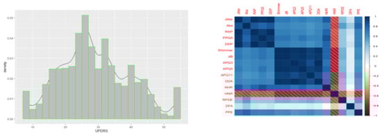
Figure 1.
(Left) Histogram and density curve of UPDRS; (right) Correlation between voice measurements.
The 16 biomedical voice measures in the PD data include several measurements of variation in fundamental frequency (Jitter, Jitter (Abs), Jitter:RAP, Jitter:PPQ5, and Jitter:DDP), several measurements of variation in amplitude (Shimmer, Shimmer (dB), Shimmer:APQ3, Shimmer:APQ5, Shimmer:APQ11, and Shimmer:DDA), two measurements of the ratio of noise to tonal components in the voice (NHR and HNR), a nonlinear dynamical complexity measurement (RPDE), signal fractal scaling exponent (DFA), and a nonlinear measure of fundamental frequency variation (PPE). Our interest is to identify the biomedical voice measurements and their interactions that may effectively affect the UPDRS (Unified Parkinson Disease Rating Scale) in Parkinson’s disease patients. Figure 1 (right) shows the correlations among 16 biomedical voice measurements. As we can see from Figure 1 (right), except for variable DFA, there are strong correlations among the covariates, which makes variable selection more challenging. Therefore, the proposed additive quantile regression model with nonlinear interaction structures may provide a complete picture on how those factors and their interactions affect the distribution of UPDRS.
We first randomly generated 100 partitions of the data into training and test sets. For each training set, we select 5475 observations as training set and the remaining 400 observations as the test set. Normalization is conducted for the dataset. Also, quantile regression is used to fit the model selected by the proposed method. For comparison, we also use least square to fit the model selected by hirNet and RAMP on the training set. Finally, we evaluate the performance of these models using the fixed active sets on the corresponding test sets.
Table 5 summarizes the covariates selected by different methods. The proposed quantile-specific method reveals distinct covariate patterns across different UPDRS severity levels. At lower quantiles ( and ), the model highlights DFA and its interactions (e.g., HNRDFA, DFAPPE), suggesting that these acoustic features may be particularly relevant in the early stages of the disease. The middle quantile () incorporates additional speech markers (APQ11, RPDE), which align with conventional methods, while higher quantiles ( and ) progressively simplify to core features (HNR, dB), indicating reduced covariate dependence in advanced stages. This dynamic selection demonstrates how quantile-specific modeling can capture stage-dependent biological mechanisms while maintaining model parsimony, selecting just 3–5 main effects and 1–2 interactions per quantile, compared to hitNet’s fixed 12-variable approach. The shifting importance of HNR and DFA interactions across quantiles particularly underscores their complex, nonlinear relationships with symptom progression.
Table 5.
The covariates selected by the proposed methods.
Figure 2 and Figure 3 show the estimation results of main effects and interaction effects at . The solid lines represent the estimated effects, while the dashed lines indicate the confidence intervals obtained through a simulation-based approach. Specifically, for the chosen model, we conducted 100 repeated simulations on the dataset to derive point-wise confidence intervals for each covariate’s effect.
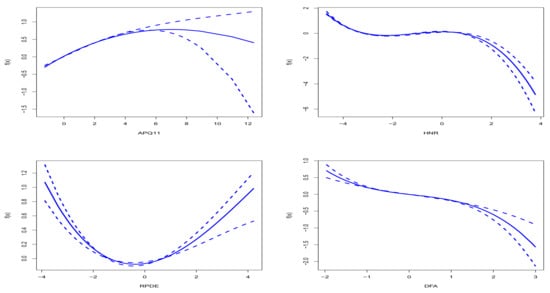
Figure 2.
Estimated main effects for the APQ11, HNR, RPDE, and DFA variables at .
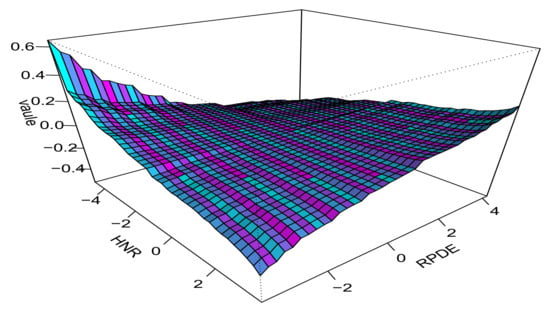
Figure 3.
Estimated interaction term for the HNR and RPDE variables at .
From Figure 2, it can be observed that, as APQ11 increases, the UPDRS score initially rises and then declines, peaking at a specific value. This inverted U-shaped relationship suggests that moderate amplitude variations are linked to more severe symptoms. For HNR, the UPDRS score decreases as the noise ratio increases, indicating that higher noise levels correlate with disease worsening. The confidence intervals around these trends confirm their statistical significance across the simulated datasets. RPDE shows a U-shaped curve, meaning that intermediate complexity levels are associated with more severe symptoms, while extreme values (high or low) indicate milder symptoms. The confidence intervals further support this nonlinear relationship, demonstrating its robustness to the data. DFA has a negative correlation with the UPDRS score: as fundamental frequency variability increases, the UPDRS score decreases, suggesting that greater variability is linked to symptom relief. The narrow confidence intervals around this trend highlight its consistency across the simulations.
Figure 3 illustrates the interaction effect between HNR and RPDE on the UPDRS score. This shows that, as HNR increases, the impact on the UPDRS score becomes more negative, especially when RPDE is at lower values, indicating a worsening in symptoms with higher noise to harmonic ratio. Conversely, for higher values of RPDE, the interaction effect stabilizes, suggesting less influence on the UPDRS score. The plot reveals a valley-like structure around the center where both HNR and RPDE are near zero, signifying minimal interaction effect. Notably, the most significant interactions occur at extreme values of either HNR or RPDE, highlighting the complex, nonlinear relationship between these variables and Parkinson’s disease symptom severity. The estimation results of the main effects and interaction effects at are presented in Appendix B.
From the results in Appendix B, it can be seen that, although the main effects selected at and are the same, their impacts on UPDRS scores differ due to nonlinear relationships or complex interactions between variables. This highlights the advantage of quantile regression, which not only captures the average trend of the dependent variable but also reveals how these effects vary across different quantiles. This method provides a more comprehensive understanding of the complex relationships between variables and helps to analyze the specific effects of variables on UPDRS under different conditions.
From the perspective of quantile-specific sparsity, the proposed method demonstrates varying levels of covariate selection across different quantiles. At lower quantiles ( and ), the model tends to select fewer covariates, focusing primarily on HNR, DFA, and PPE, which suggests a higher degree of sparsity. As the quantile increases to , the model selects more covariates, including APQ11 and RPDE, indicating a reduction in sparsity. At higher quantiles ( and ), the model again shows increased sparsity by selecting only a few key covariates such as HNR, DFA, and PPE. This pattern reflects the adaptability of the proposed method in capturing the specific characteristics of the data distribution at different quantiles, thereby achieving optimal sparsity tailored to each quantile level.
Table 6 compares the average RMSE and model sizes across 100 datasets for three methods: the proposed quantile-based approach (evaluated at ), RAMP, and hirNet. The results show that our method outperforms the others in predictive accuracy, particularly at , where it achieves the lowest RMSE of 0.858, outperforming RAMP (0.878) and hirNet (0.887). Additionally, the proposed method uses much smaller models, with only 2.3–5.0 variables, compared to hirNet’s larger model with 18.39 variables. This reduction in model size highlights the method’s efficiency without sacrificing predictive power. The method also performs consistently well across different quantiles, with a particularly strong result at (RMSE = 0.873), though the RMSE at is slightly higher (1.00), showing some variation in performance across quantiles. Furthermore, models that include interaction terms perform better than those with only main effects, emphasizing the importance of interaction effects in the model. In conclusion, the proposed method strikes an optimal balance between prediction accuracy, model simplicity, and computational efficiency, making it ideal for applications that require both interpretability and strong predictive performance.
Table 6.
The average RMSE over the 100 data sets.
6. Conclusions
We explore the variable selection for additive quantile regression with interactions. We fit the model using the sparsity smooth penalty function and add the regularization algorithm under the marginality principle to the additive quantile regression with interactions, which can select main and interaction effects simultaneously while keeping either the strong or weak heredity constraints. We demonstrate theoretical properties of the proposed method for additive quantile regression with interactions. Simulation studies demonstrate good performance of the proposed model and method.
Also, we applied the proposed method to the Parkinson’s disease (PD) data; our method successfully validates the important finding in the literature that frequent, remote, and accurate UPDRS tracking as a novel PD treatment could be effective in telemonitoring frameworks for PD symptom monitoring and large-scale clinical trials.
Author Contributions
Y.B.: Conceptualization, Formal analysis, Methodology, Software, Writing—original draft, Data curation; J.J.: Formal analysis, Methodology, Writing—review and editing; M.T.: Supervision, Funding acquisition. All authors have read and agreed to the published version of the manuscript.
Funding
The work was partially supported by the Beijing Natural Science Foundation (No.1242005).
Data Availability Statement
The dataset used in this study is publicly available at https://www.worldbank.org/en/home (accessed on 1 June 2023).
Conflicts of Interest
The authors declare no conflictw of interest.
Appendix A. Proof of the Theorem
Appendix A.1. Proof of Theorem 1
Throughout the proof, if is a vector, we use the norms and . For a function f on , we denote its norm by . We write and write in the same fashion. Let . Note that we can express ; alternatively, we can express it as . By the identifiability of the model, we must have .
Notice that
where and . Define the minimizers under the transformation as
Let be a sequence of positive numbers and define
Define
and
where .
Lemma A1.
Let . If Conditions (A1)–(A4) are satisfied, then, for any positive constant L,
Proof.
Note that
Using Knight’s identity
we have
Therefore, . We have
for some positive constant C, where is an diagonal matrix with denoting the conditional density function of given evaluated at zero. Therefore, for some positive constant C and all n sufficiently large. By Bernstein’s inequality, for all n sufficiently large,
which converges to 0 as by Conditions (A3) and (A4). Note that the upper bound does not depend on , so the above bound also holds unconditionally. □
Lemma A2.
Suppose that Conditions (A1)–(A4) hold. Then, for any sequence with , we have
Using the similar arguments as described to prove Lemma 3.2 in [40], Lemma A2 can be proven.
Proof.
For Theorem 1(1), we first prove that, , there exists a such that
Note that
where the definition of is clear from the context. First, we can see that by Lemma A1.
For , we have
where the definition of is clear from the context. Note that for all , where B is the constant in the assumption (A2). Let . By Condition (A3), we have . Consequently, we can take a constant such that by Condition (A3) and Lemma A2. For , we have
where . Based on Condition (A3), there exists a finite constant , such that with the probability approaching one. Combining Condition (A2) and the Cauchy–Schwarz inequality, we obtain
We next evaluate , noting that and
Therefore, . Hence, for L sufficiently large, the quadratic term will dominate and has asymptotically a lower bound . By convexity, this implies . From the definition of , it follows that . This completes the proof of Theorem 1 (a).
The proof of Theorem 1 (b) is immediate since and . □
Appendix A.2. Proof of Theorem 2
Proof.
Note that is the oracle estimator. Our goal is to prove that is a local minimizer of . The gradient function of is not applicable in the proof because the check loss function is not differentiable at zero. We derive it directly from a certain lower bound of the difference of two check loss functions.
Suppose that there exists an index and , such that and . That is, and . Let be the vector obtained with and being replaced by 0. Since for any , then
where . By simple calculation, one has that . Therefore, . For , from Conditions (A2) and (A3), we have
where for some positive constant . The last equality follows by observing that . This implies that . Therefore, . By , , and , we have that will dominate. Therefore, with probability tending to one, which contradicts the fact that is the minimizer of . Similarly, the same results are proven under weak heredity. This completes the proof of Theorem 2. □
Appendix A.3. Proof of Theorem 3
Lemma A3.
Let be independent random variable with values in some space and let Γ be a class of real-valued functions on , satisfying, for some positive constants and ,
Define . Then, for ,
For the details of this proof, see [41].
Proof.
Define . We can write . By Lemma A3, we have
with probability at least for . Based on the subadditivity and inequality , we have
Then, with probability at least , we have
Let be the collection of all differences . The bracketing number is the minimum number of -brackets over , where . We can construct 2-brackets over by taking difference for the upper and lower bounds. Therefore, the bracketing numbers are bounded by the squares of the bracketing numbers . For , by theorem 19.5 in [42], there exists a finite number such that
where is the bracketing integral. The envelope function M can be taken as equal to the supremum of the absolute values of the upper and lower bounds of finitely many brackets over . Based on Theorem 19.5 in [42], the second term on the right is bounded by and hence converges to zero as . Given , there exists a constant K such that, for Sobolev space ,
Note that, and , where and . Reference [43] implies that the bracketing integral of Sobolev space and is bounded. Then,
By the convexity of , there exists such that and . Let and . Then, Equation (A1) implies that
with probability at least as . From the above, we have and that there exists such that . Under the assumption that the regression function is bounded, it follows, for and , that
where . Reference [13] also shows that the Lasso is persistent when p grows polynomially in n. Furthermore, according to the definition of , we have and . Let . Since always holds, the probability of is 1. Note that . Therefore, with probability at least . Similarly, the same results are proved under weak heredity. □
Appendix B. Estimated Results at τ = 0.1, 0.25, 0.75, 0.9 in Applications
Figure A1 illustrates the effects of HNR, RPDE, and DFA on the UPDRS score at . As HNR increases, the UPDRS score significantly decreases, showing a nonlinear relationship, where higher noise-to-harmonic ratios are associated with milder symptoms. RPDE exhibits a clear U-shaped curve, indicating that extreme values correspond to more severe symptoms, while intermediate values are associated with milder symptoms, reflecting a nonlinear effect pattern. DFA shows a negative correlation, with UPDRS scores decreasing as DFA increases, again revealing a nonlinear trend, suggesting that increased fundamental frequency variability may help to alleviate symptoms.
Figure A2 shows the interaction effect between HNR and DFA at , revealing a nonlinear relationship. When HNR is low and DFA is high, the UPDRS score is higher; as HNR increases, the UPDRS score decreases. However, when HNR is high and DFA is low, the score increases again. This suggests that the effects of HNR and DFA on the UPDRS score are complex and interdependent, highlighting the importance of understanding and analyzing the interactions between these variables.
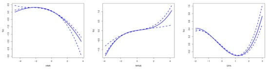
Figure A1.
Estimated main effects for the HNR, RPDE, and DFA variables at .
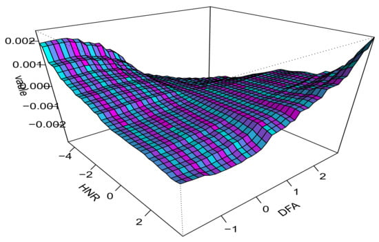
Figure A2.
Estimated interaction between HNR and DFA at .
Figure A3 illustrates the estimated main effect trends of three acoustic features—HNR, DFA, and PPE—at . Under this condition, as HNR increases, its impact on the analysis first rises slightly and then drops rapidly, indicating that the purity of the speech signal influences recognition but with diminishing returns beyond a certain point. DFA reveals an optimal fluctuation pattern, after which its ability to reflect health status declines. PPE shows that the randomness and complexity of the speech signal also have an optimal range, beyond which the effect weakens. Overall, the variations in these features highlight their potential applications in fields such as disease diagnosis, where analyzing these acoustic characteristics can assist in medical diagnostics and improve accuracy.
Figure A4 illustrates the estimated interaction between DFA and PPE at , presented through a 3D surface plot. As DFA and PPE values vary, their interaction significantly impacts the overall effect. Specifically, when DFA is at a low level, the overall effect initially increases slowly and then drops rapidly as PPE increases. In contrast, when DFA is high, this trend becomes more gradual, indicating a more complex interaction pattern. This suggests that the influence of their interaction varies significantly across different DFA and PPE combinations. For instance, in certain combinations, their interaction can more accurately reflect changes in health status within speech signals, which is important for disease diagnosis and improving speech processing technologies. Overall, the figure highlights the nonlinear interaction between DFA and PPE and its potential applications.
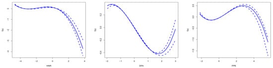
Figure A3.
Estimated main effects for the HNR, DFA, and PPE variables at .
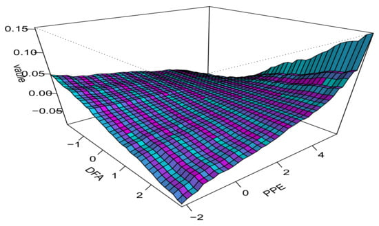
Figure A4.
Estimated interaction between DFA and PPE at .
Figure A5 illustrates the estimated main effects of three variables HNR, DFA, and PPE at . From the figure, it can be observed that, as the HNR value increases, its impact on the overall effect first rises and then rapidly decreases. The change in DFA values shows a similar trend, but the decline is more gradual. Meanwhile, the PPE value exhibits a distinct peak before gradually decreasing. These variations in the features highlight their significance in practical applications, particularly in disease diagnosis and speech processing fields.
Figure A6 illustrates the estimated interaction effects between HNR and DFA, as well as between HNR and PPE at . From the figure, it can be observed that the interaction between HNR and DFA exhibits a complex nonlinear relationship, with the overall effect first increasing and then decreasing as the HNR value rises, showing a distinct fluctuation pattern. Similarly, the interaction between HNR and PPE also displays a complex pattern, but with more pronounced changes, particularly when the PPE value is high, leading to more significant variations in the overall effect.
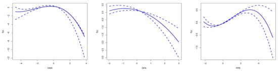
Figure A5.
Estimated main effects for the HNR and DFA variables at .
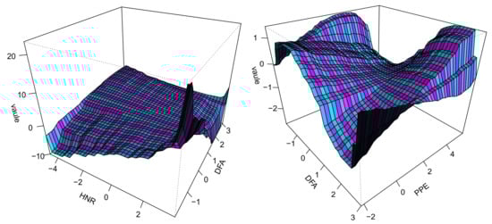
Figure A6.
Estimated interaction effects between HNR and DFA, as well as the interaction effect between HNR and PPE variables at .
Figure A7 provides the effects of dB and HNR on the UPDRS score at . The main effect of dB presents a U-shaped curve, indicating that both extremely high and low dB values lead to higher UPDRS scores, with lower scores at intermediate values. This emphasizes the importance of moderate changes in sound levels and their nonlinear effects. HNR also shows an inverted U-shaped curve, indicating that moderate HNR values are associated with the most severe symptoms, with this nonlinear relationship being particularly prominent at higher quantiles. These findings highlight the complex nonlinear effects of different variables on the UPDRS score, providing valuable insights for understanding Parkinson’s disease symptoms.
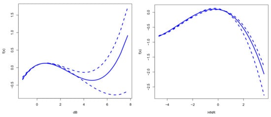
Figure A7.
Estimated main effects for the dB and HNR variables at .
References
- Koenker, R.; Bassett, G. Regression quantiles. Econometrica 1978, 46, 33–50. [Google Scholar] [CrossRef]
- Nelder, J.A. A reformulation of linear models. J. R. Stat. Soc. Ser. A (Gen.) 1977, 140, 48–63. [Google Scholar] [CrossRef]
- McCullagh, P.; Nelder, J. Monographs on Statistics and Applied Probability; Chapman & Hall: London, UK, 1989. [Google Scholar]
- De Gooijer, J.G.; Zerom, D. On additive conditional quantiles with high-dimensional covariates. J. Am. Stat. Assoc. 2003, 98, 135–146. [Google Scholar] [CrossRef]
- Cheng, Y.; De Gooijer, J.G.; Zerom, D. Efficient estimation of an additive quantile regression model. Scand. J. Stat. 2011, 38, 46–62. [Google Scholar] [CrossRef]
- Lee, Y.K.; Mammen, E.; Park, B.U. Backfitting and smooth backfitting for additive quantile models. Ann. Stat. 2010, 38, 2857–2883. [Google Scholar] [CrossRef]
- Horowitz, J.L.; Lee, S. Nonparametric estimation of an additive quantile regression model. J. Am. Stat. Assoc. 2005, 100, 1238–1249. [Google Scholar] [CrossRef]
- Sherwood, B.; Maidman, A. Additive nonlinear quantile regression in ultra-high dimension. J. Mach. Learn. Res. 2022, 23, 1–47. [Google Scholar]
- Zhao, W.; Li, R.; Lian, H. Estimation and variable selection of quantile partially linear additive models for correlated data. J. Stat. Comput. Simul. 2024, 94, 315–345. [Google Scholar] [CrossRef]
- Cui, X.; Zhao, W. Pursuit of dynamic structure in quantile additive models with longitudinal data. Comput. Stat. Data Anal. 2019, 130, 42–60. [Google Scholar] [CrossRef]
- Lin, Y.; Zhang, H.H. Component selection and smoothing in multivariate nonparametric regression. Ann. Stat. 2006, 34, 2272–2297. [Google Scholar] [CrossRef]
- Storlie, C.B.; Bondell, H.D.; Reich, B.J.; Zhang, H.H. Surface estimation, variable selection, and the nonparametric oracle property. Stat. Sin. 2011, 21, 679–705. [Google Scholar] [CrossRef] [PubMed]
- Radchenko, P.; James, G.M. Variable selection using adaptive nonlinear interaction structures in high dimensions. J. Am. Stat. Assoc. 2010, 105, 1541–1553. [Google Scholar] [CrossRef]
- Efron, B.; Hastie, T.; Johnstone, I.; Tibshirani, R. Least angle regression. Ann. Stat. 2004, 32, 407–499. [Google Scholar] [CrossRef]
- Wu, T.T.; Chen, Y.F.; Hastie, T.; Sobel, E.; Lange, K. Genome-wide association analysis by lasso penalized logistic regression. Bioinformatics 2009, 25, 714–721. [Google Scholar] [CrossRef]
- Zhao, P.; Rocha, G.; Yu, B. The composite absolute penalties family for grouped and hierarchical variable selection. Ann. Stat. 2009, 37, 3468–3497. [Google Scholar] [CrossRef]
- Yuan, M.; Joseph, V.R.; Zou, H. Structured variable selection and estimation. Ann. Appl. Stat. 2009, 3, 1738–1757. [Google Scholar] [CrossRef]
- Choi, N.H.; Li, W.; Zhu, J. Variable selection with the strong heredity constraint and its oracle property. J. Am. Stat. Assoc. 2010, 105, 354–364. [Google Scholar] [CrossRef]
- Bien, J.; Taylor, J.; Tibshirani, R. A lasso for hierarchical interactions. Ann. Stat. 2013, 41, 1111–1141. [Google Scholar] [CrossRef]
- She, Y.; Wang, Z.F.; Jiang, H. Group regularized estimation under structural hierarchy. J. Am. Stat. Assoc. 2018, 113, 445–454. [Google Scholar] [CrossRef]
- Hao, N.; Feng, Y.; Zhang, H.H. Model Selection for High Dimensional Quadratic Regression via Regularization. J. Am. Stat. Assoc. 2018, 113, 615–625. [Google Scholar] [CrossRef]
- Liu, C.; Ma, J.; Amos, C.I. Bayesian variable selection for hierarchical gene–environment and gene–gene interactions. Hum. Genet. 2015, 134, 23–36. [Google Scholar] [CrossRef] [PubMed]
- Yang, Y.; Basu, S.; Zhang, L. A Bayesian hierarchical variable selection prior for pathway-based GWAS using summary statistics. Stat. Med. 2020, 39, 724–739. [Google Scholar] [CrossRef] [PubMed]
- Kim, J.E.A. Bayesian variable selection with strong heredity constraints. J. Korean Stat. Soc. 2018, 47, 314–329. [Google Scholar] [CrossRef]
- Li, Y.; Wang, N.; Carroll, R.J. Generalized functional linear models with semiparametric single-index interactions. J. Am. Stat. Assoc. 2010, 105, 621–633. [Google Scholar] [CrossRef]
- Li, Y.; Liu, J.S. Robust variable and interaction selection for logistic regression and multiple index models. J. Am. Stat. Assoc. 2019, 114, 271–286. [Google Scholar] [CrossRef]
- Liu, Y.; Li, Y.; Carroll, R.J. Predictive functional linear models with diverging number of semiparametric single-index interactions. J. Econom. 2021, 230, 221–239. [Google Scholar] [CrossRef]
- Liu, H.; You, J.; Cao, J. A Dynamic Interaction Semiparametric Function-on-Scalar Model. J. Am. Stat. Assoc. 2021, 118, 360–373. [Google Scholar] [CrossRef]
- Yu, K.; Lu, Z. Local linear additive quantile regression. Scand. J. Stat. 2004, 31, 333–346. [Google Scholar] [CrossRef]
- Noh, H.; Lee, E.R. Component selection in additive quantile regression models. J. Korean Stat. Soc. 2014, 43, 439–452. [Google Scholar] [CrossRef]
- Wood, S.N. P-splines with derivative based penalties and tensor product smoothing of unevenly distributed data. Stat. Comput. 2017, 27, 985–989. [Google Scholar] [CrossRef]
- Eilers, P.H.C.; Marx, B.D. Flexible smoothing with B-splines and penalties. Stat. Sci. 1996, 11, 89–102. [Google Scholar] [CrossRef]
- Meier, L.; van de Geer, S.; Buehlmann, P. High-dimensional additive modeling. Ann. Stat. 2009, 37, 3779–3821. [Google Scholar] [CrossRef]
- Fan, Y.; Tang, C.Y. Tuning parameter selection in high dimensional penalized likelihood. J. R. Stat. Soc. Ser. B 2013, 75, 531–552. [Google Scholar] [CrossRef]
- Greenshtein, E.; Ritov, Y. Persistence in high-dimensional linear predictor selection and the virtue of overparametrization. Bernoulli 2004, 10, 971–988. [Google Scholar] [CrossRef]
- Jiang, L.; Bondell, H.; Wang, H. Interquantile shrinkage and variable selection in quantile regression. Comput. Stat. Data Anal. 2014, 69, 208–219. [Google Scholar] [CrossRef]
- Zou, H.; Ming, Y. Composite quantile regression and the oracle model selection theory. Ann. Stat. 2008, 36, 1108–1126. [Google Scholar] [CrossRef]
- Kohns, D.; Szendrei, T. Horseshoe prior Bayesian quantile regression. J. R. Stat. Soc. Ser. C Appl. Stat. 2024, 73, 193–220. [Google Scholar] [CrossRef]
- Tsanas, A.; Little, M.A.; McSharry, P.E.; Ramig, L.O. Accurate telemonitoring of parkinson’s disease progression by noninvasive speech tests. IEEE Trans. Bio-Med. Eng. 2010, 57, 884–893. [Google Scholar] [CrossRef]
- He, X.M.; Shi, P. Convergence rate of B-spline estimators of nonparametric conditional quantile functions. J. Nonparametr. Stat. 1994, 3, 299–308. [Google Scholar] [CrossRef]
- Bousquet, O. A Bennett concentration inequality and its application to suprema of empirical processes. Comptes Rendus Math. 2002, 334, 495–500. [Google Scholar] [CrossRef]
- Vaart, A. Asymptotic Statistics; Cambridge University Press: Cambridge, UK, 1990. [Google Scholar]
- Birman, M.; Solomjak, M.Z. Piecewise-polynomial approximations of functions of the classes. Math. USSR-Sb. 1967, 2, 295–317. [Google Scholar] [CrossRef]
Disclaimer/Publisher’s Note: The statements, opinions and data contained in all publications are solely those of the individual author(s) and contributor(s) and not of MDPI and/or the editor(s). MDPI and/or the editor(s) disclaim responsibility for any injury to people or property resulting from any ideas, methods, instructions or products referred to in the content. |
© 2025 by the authors. Licensee MDPI, Basel, Switzerland. This article is an open access article distributed under the terms and conditions of the Creative Commons Attribution (CC BY) license (https://creativecommons.org/licenses/by/4.0/).