Transient Post-Buckling of Microfluid-Conveying FG-CNTs Cylindrical Microshells Embedded in Kerr Foundation and Exposed to a 2D Magnetic Field

Abstract

Dynamic post-buckling behavior of microscale cylindrical shells reinforced with functionally graded carbon nanotubes (FG-CNTs) and conveying microfluid is discussed for the first time. The microshell is embedded in a Kerr foundation and subjected to an axial compressive load and a two-dimensional magnetic field effect. CNTs dispersion across the shell thickness follows a power law, with five distribution types developed. The modified couple stress theory is applied to incorporate the small-size effect using a single material parameter. Furthermore, the Knudsen number is used to address the small-size effect on the microfluid. The external force between the magnetic fluid and microshell is modeled by applying the Navier–Stokes equation depending on the fluid velocity. Nonlinear motion equations of the present model are derived using Hamilton’s principle, containing the Lorentz magnetic force. According to the Galerkin method, the equations of motion are transformed into an algebraic system to be solved, determining the post-buckling paths. Numerical results indicate that the presence of the magnetic field, CNT reinforcement, and fluid flow improves the load-bearing performance of the cylindrical microshells. Also, many new parametric effects on the post-buckling curves of the FG-CNT microshells have been discovered, including the shell geometry, magnetic field direction, length scale parameter, Knudsen number, and CNT distribution types.

1. Introduction

Carbon nanotubes represent a novel class of materials with outstanding stiffness and strength [1]. Due to their superior mechanical, electrical, and physical qualities CNTs have recently been employed to reinforce several matrices, including metal filler, ceramic, and polymer. Carbon nanotubes come in two varieties: single-walled (abbreviated SWCNTs) and multiwalled (abbreviated MWCNTs), which are composed of several concentric SWCNTs. Although MWCNTs are comparatively weaker, both forms are utilized to strengthen composites [2]. According to Sun et al. [3], the ultimate tensile strength of a SWCNT-nickel nanocomposite was 320% greater than that of pure nickel, whereas it was 270% stronger for a MWCNT-nickel nanocomposite. As a result, SWCNTs enhance matrix strength more successfully than MWCNTs, and they might be a better choice for reinforcement. The uniform or random distribution of reinforcement in traditional composites results in uniform mechanical characteristics across the material. However, because of the uneven distribution of reinforcement, functionally graded material will undergo processing that results in a spatial variance in characteristics. On the basis of this idea, graded distribution strategies are created for materials reinforced with carbon nanotubes. Zhu et al. [4] analyzed the natural frequency and bending of composite plates strengthened with CNTs employing the first-order plate theory to formulate the displacements and the finite element technique to solve the governing equations. Concurrently, in Alibeigloo [5], the thermo-electric bending analysis of the rectangular plate reinforced with CNTs integrated with piezoelectric layers was illustrated, employing the 3D elasticity theory. Sobhy and Radwan [6,7] studied the effects of the 2D magnetic field and hygrothermal conditions on the bending and buckling of a viscoelastic sandwich rectangular plate reinforced with CNTs based on a higher-order shear deformation theory. In addition, Sobhy and Zenkour [8] investigated the magnetic and humidity effects on the vibration, mechanical buckling, and thermal buckling of viscoelastic sandwich nanobeams with FG-CNTs face layers embedded in visco-Pasternak foundation. Ghasemi et al. [9] analyzed the dynamic response of a hybrid laminated nanocomposite truncated conical shell strengthened with FG graphene platelets and FG-CNTs via a higher-order shell theory and the differential quadrature method (DQM). Furthermore, Zhao et al. [10] discussed the buckling temperature of the conical-conical shells reinforced with CNTs based on the first-order shell theory (FST), von Karman’s nonlinearity (vKN), and the DQM. Additionally, You et al. [11] employed the FST, vKN, and DQM to elucidate the stability analysis of FG-CNTs conical-cylindrical shells exposed to axial compressive load, thermal load, and lateral compressive force. In recent years, numerous studies have focused on the linear [12,13,14] and nonlinear [15,16] vibration behavior of structures reinforced with functionally graded carbon nanotubes.

Fluid-conveying cylindrical shells are vital parts of biological and engineering systems [17]. Examples include arterial blood flow [18], subsea and underground oil pipelines [19], steel conduits for a power plant [20], pulmonary airways [21], control and monitoring tubes, aerospace and power-plant industries, shells used in storage tanks and heat exchangers, etc. [22]. The interaction between the fluid and the shell structure makes it essential to comprehend their dynamic properties. A significant problem in many industrial applications is the fluid-structure interaction. Complex behaviors are produced when fluid flow alters the mass, stiffness, and damping of the shells. Divergence and flutter are examples of instability that can happen as flow velocity rises. Studying the dynamics and enhancing design techniques are crucial to preventing undesired behaviors. In recent decades, numerous research studies have examined the different behaviors of the fluid-conveying cylindrical shells, such as [23,24]. Based on the finite element method (FEM)and the 3D elasticity theory, Zhang et al. [25] predicted the natural frequencies of cylindrical shells conveying fluid. Based on the Flügge shell theory, the nonlinear model of the circular cylindrical shells is introduced by [26] to investigate the nonlinear dynamics response of the clamped-free shells subjected to axial internal flow. Mohammadimehr and Mehrabi [27] employed Reddy’s shell theory and the DQM to illustrate the effects of the thermo-mechanical-magnetic loads on the natural frequency of microscale sandwich axisymmetric cylindrical shells having CNTs-reinforced face layers and porous core conveying fluid. The influence of the material length scale parameter and viscoelastic coefficient on the vibration of cylindrical microshells conveying fluid was demonstrated by Rashvand et al. [28] based on the modified couple stress theory and the classical shell theory. The piezoelectric effect on the vibration response of functionally graded (FG) cylindrical shells integrated with piezoelectric sheets and subjected to axial internal flow was studied by Ebrahimi [29]. The study utilized 3D elasticity theory to derive the motion equations, which were solved using the state-space approach. At the same time, Abdollahi et al. [30] illustrated the nonlinear vibration of spinning cylindrical shells with different rotation speeds conveying incompressible fluid based on the Sanders-–Koiter kinematic assumptions and Runge–Kutta technique. Further, Al-Furjan et al. [31] utilized the first-order shear deformable theory to analyze the vibration control of spinning nanocomposite reinforced cylindrical microshells integrated with two piezoelectric layers and conveying viscous fluid. Recently, Hoang et al. [32] elucidated the nonlinear vibration of FG cylindrical shells carrying incompressible fluid embedded in a non-uniform elastic medium. The motion equations were derived based on the classical shell theory and von Karman’s nonlinear relations and then solved via Galerkin and fourth-order Runge-Kutta methods. However, Sobhy [33] used a higher-order beam theory to investigate the nonlinear bending and wave propagation in a nanocomposite microtube surrounded by a Kerr substrate and containing viscous fluid. The nonlinear dynamical responses of the graphene oxide powder reinforced cylindrical shell carrying incompressible fluid were discussed by Zhang et al. [34], employing the classical shell theory.

Despite extensive studies on the vibration, buckling, and dynamic behaviors of fluid-conveying CNT-reinforced structures, critical gaps remain. In particular, the dynamic post-buckling response of microscale cylindrical shells reinforced with FG-CNTs under the combined influences of microfluid flow, a Kerr-type elastic foundation, and a two-dimensional magnetic field has not been previously investigated. Moreover, existing works often neglect essential microscale effects, such as the material length scale parameter and the Knudsen number for microfluid dynamics, which are crucial for accurate modeling at the microscale. The practical significance of this study lies in providing a more comprehensive framework for analyzing the stability of advanced microsystems, with potential applications in biomedical, aerospace, and nano-engineering fields. Consequently, the novelty of the current analysis can be summarized as follows: (a) The transient post-buckling response of FG-CNTs cylindrical microshells containing flowing-fluid is discussed, accounting for asymmetric deformations. (b) The influence of the Lorentz force, induced by the 2D magnetic field, on the shells and fluid is considered. (c) The sinusoidal shear deformation shell theory is presented, incorporating the shallowness effect, and the von Karman geometrical nonlinearity is introduced to formulate the strain-displacement relations. (d) The influence of small-scale effects on microtubes and microfluid is addressed by applying the modified couple stress theory and accounting for the Knudsen number, respectively. The effective material properties of the composite shells are determined using the mixture rule, considering five distributions of CNTs by thickness. The motion equations are constructed based on Hamilton’s principle. The conducted equations are then solved using Galerkin’s method to deduce the transient post-buckling path of the composite microshells. A comparison study is conducted between the results obtained and those available in the literature. Additionally, several examples are presented to illustrate the effects of different parameters such as the average flow velocity, Knudsen number, Lorentz force, magnetic field direction, CNTs volume fraction, material parameter, radius-to-thickness ratio, and length-to-radius ratio on the post-buckling curves.

2. Formulation

Consider a composite cylindrical shell with a middle surface radius a, thickness H, and length L containing flowing-incompressible fluid as shown in Figure 1. The deformation of the shell is modeled based on the cylindrical coordinate system ($x,\theta ,z$). The microshell is surrounded by Kerr foundation, which is emulated by $K_l$, $K_s$, and $K_u$ corresponding to lower springs stiffness, shear foundation stiffness, and upper springs stiffness, respectively, as shown in Figure 2.

2.1. Displacement Field

Considering the higher-order shear deformation of the shell and the shallowness term $z/a$, the displacement components at a point $(x,\theta ,z)$ are given as [35,36]:

$$\begin{array}{cc}\hfill & V_x(x,\theta ,z,t)=U_x(x,\theta ,t)-z{W}_{0,x}+\psi \left(z\right){\mathrm{\Phi }}_x(x,\theta ,t)\hfill \\ \hfill & V_{\theta }(x,\theta ,z,t)=\left(1+{\displaystyle \frac{z}{a}}\right)U_{\theta }(x,\theta ,t)-{\displaystyle \frac{z}{a}}{W}_{0,\theta }+\psi \left(z\right){\mathrm{\Phi }}_{\theta }(x,\theta ,t)\hfill \\ \hfill & V_z(x,\theta ,z,t)=W_0(x,\theta ,t),\hfill \end{array}$$

(1)

where $U_x$, $U_{\theta }$, and $W_0$ represent the displacement components at $z=0$; ${\mathrm{\Phi }}_x$ and ${\mathrm{\Phi }}_{\theta }$ are the rotations about the x- and $\theta$-axes, and $f_{,i}=\partial f/\partial i,i=x,\theta ,z,t$. Additionally, $\psi \left(z\right)$ is the sinusoidal shape function given as

$$\psi \left(z\right)={\displaystyle \frac{H}{\pi }}sin\left({\displaystyle \frac{\pi }{H}}z\right).$$

(2)

2.2. Strain-Displacement Relations

Using von Karman’s model, the strain components associated with the above displacement are expressed as:

$$\begin{array}{c}\hfill \epsilon ={\epsilon }^{\left(0\right)}+z{\epsilon }^{\left(1\right)}+\psi \left(z\right){\epsilon }^{\left(2\right)}+{\psi }^{\prime }\left(z\right){\epsilon }^{\left(3\right)},{\psi }^{\prime }\left(z\right)=cos\left({\displaystyle \frac{\pi }{H}}z\right),\end{array}$$

(3)

where

$$\begin{array}{cc}\hfill & \epsilon ={\left\{{\epsilon }_x{\epsilon }_{\theta }{\epsilon }_{\theta z}{\epsilon }_{xz}{\epsilon }_{x\theta }\right\}}^T,\hfill \\ \hfill & {\epsilon }^{\left(0\right)}={{\left\{{\epsilon }_x{\epsilon }_{\theta }00{\epsilon }_{x\theta }\right\}}^{\left(0\right)}}^T,\hfill \\ \hfill & {\epsilon }^{\left(1\right)}={{\left\{{\epsilon }_x{\epsilon }_{\theta }{\epsilon }_{\theta z}0{\epsilon }_{x\theta }\right\}}^{\left(1\right)}}^T,\hfill \\ \hfill & {\epsilon }^{\left(2\right)}={{\left\{{\epsilon }_x{\epsilon }_{\theta }{\epsilon }_{\theta z}0{\epsilon }_{x\theta }\right\}}^{\left(2\right)}}^T,\hfill \\ \hfill & {\epsilon }^{\left(3\right)}={{\left\{00{\epsilon }_{\theta z}{\epsilon }_{xz}0\right\}}^{\left(3\right)}}^T,\hfill \end{array}$$

(4)

in which

$$\begin{array}{cc}\hfill & {\epsilon }_x^{\left(0\right)}=U_{x,x}+{\displaystyle \frac{1}{2}}{W}_{0,x}^2,{\epsilon }_{\theta }^{\left(0\right)}={\displaystyle \frac{1}{a}}{U}_{\theta ,\theta }+{\displaystyle \frac{W_0}{a}}+{\displaystyle \frac{1}{2a^2}}{W}_{0,\theta }^2,\hfill \\ \hfill & {\epsilon }_{x\theta }^{\left(0\right)}={\displaystyle \frac{1}{a}}{U}_{x,\theta }+U_{\theta ,x}+{\displaystyle \frac{1}{a}}{W}_{0,x}{W}_{0,\theta },{\epsilon }_x^{\left(1\right)}=-W_{0,xx},\hfill \\ \hfill & {\epsilon }_{\theta }^{\left(1\right)}={\displaystyle \frac{1}{a^2}}{U}_{\theta ,\theta }-{\displaystyle \frac{1}{a^2}}{W}_{0,\theta \theta },{\epsilon }_{\theta z}^{\left(1\right)}={\displaystyle \frac{1}{a^2}}{W}_{0,\theta }-{\displaystyle \frac{U_{\theta }}{a^2}},{\epsilon }_{x\theta }^{\left(1\right)}={\displaystyle \frac{1}{a}}{U}_{\theta ,x}-{\displaystyle \frac{2}{a}}{W}_{0,x\theta },\hfill \\ \hfill & {\epsilon }_x^{\left(2\right)}={\mathrm{\Phi }}_{x,x},{\epsilon }_{\theta }^{\left(2\right)}={\displaystyle \frac{1}{a}}{\mathrm{\Phi }}_{\theta ,\theta },{\epsilon }_{\theta z}^{\left(2\right)}=-{\displaystyle \frac{1}{a}}{\mathrm{\Phi }}_{\theta },{\epsilon }_{x\theta }^{\left(2\right)}={\mathrm{\Phi }}_{\theta ,x}+{\displaystyle \frac{1}{a}}{\mathrm{\Phi }}_{x,\theta },\hfill \\ \hfill & {\epsilon }_{\theta z}^{\left(3\right)}={\mathrm{\Phi }}_{\theta },{\epsilon }_{xz}^{\left(3\right)}={\mathrm{\Phi }}_x.\hfill \end{array}$$

(5)

2.3. Rotation and Curvature Tensors

The rotation tensor $\varpi$ is related with the displacement vector $\mathbf{V}$ as [37]:

$$\varpi ={\displaystyle \frac{1}{2}}\nabla \times \mathbf{V}.$$

(6)

Substituting Equation (1) into Equation (6) yields

$$\begin{array}{cc}\hfill & {\varpi }_x={\displaystyle \frac{1}{a}}{W}_{0,\theta }-{\displaystyle \frac{U_{\theta }}{2a}}-{\displaystyle \frac{1}{2}}{\psi }^{\prime }{\mathrm{\Phi }}_{\theta },{\varpi }_{\theta }=-W_{0,x}+{\displaystyle \frac{1}{2}}{\psi }^{\prime }{\mathrm{\Phi }}_x,\hfill \\ \hfill & {\varpi }_z={\displaystyle \frac{1}{2}}\left(U_{\theta ,x}-{\displaystyle \frac{1}{a}}{U}_{x,\theta }\right)+{\displaystyle \frac{1}{2a}}z{U}_{\theta ,x}+{\displaystyle \frac{1}{2}}\psi \left({\mathrm{\Phi }}_{\theta ,x}-{\displaystyle \frac{1}{a}}{\mathrm{\Phi }}_{x,\theta }\right).\hfill \end{array}$$

(7)

Concurrently, the symmetric curvature tensor $\mathrm{\Theta }$ can be expressed as [33,37]:

$$\begin{array}{c}\hfill \mathrm{\Theta }={\displaystyle \frac{1}{2}}\left[\nabla \varpi +{(\nabla \varpi )}^T\right].\end{array}$$

(8)

Inserting Equation (7) into Equation (8) yields

$$\mathrm{\Theta }={\mathrm{\Theta }}^{\left(0\right)}+z{\mathrm{\Theta }}^{\left(1\right)}+\psi {\mathrm{\Theta }}^{\left(2\right)}+{\psi }^{\prime }{\mathrm{\Theta }}^{\left(3\right)}+{\psi }^{″}{\mathrm{\Theta }}^{\left(4\right)},$$

(9)

where

$$\begin{array}{cc}\hfill & \mathrm{\Theta }={\left\{{\mathrm{\Theta }}_x{\mathrm{\Theta }}_{\theta }{\mathrm{\Theta }}_z{\mathrm{\Theta }}_{\theta z}{\mathrm{\Theta }}_{xz}{\mathrm{\Theta }}_{x\theta }\right\}}^T,\hfill \\ \hfill & {\mathrm{\Theta }}^{\left(0\right)}={{\left\{{\mathrm{\Theta }}_x{\mathrm{\Theta }}_{\theta }{\mathrm{\Theta }}_z{\mathrm{\Theta }}_{\theta z}{\mathrm{\Theta }}_{xz}{\mathrm{\Theta }}_{x\theta }\right\}}^{\left(0\right)}}^T,\hfill \\ \hfill & {\mathrm{\Theta }}^{\left(1\right)}={{\left\{0{\mathrm{\Theta }}_{\theta }0{\mathrm{\Theta }}_{\theta z}{\mathrm{\Theta }}_{xz}0\right\}}^{\left(1\right)}}^T,\hfill \\ \hfill & {\mathrm{\Theta }}^{\left(2\right)}={{\left\{0{\mathrm{\Theta }}_{\theta }0{\mathrm{\Theta }}_{\theta z}{\mathrm{\Theta }}_{xz}0\right\}}^{\left(2\right)}}^T,\hfill \\ \hfill & {\mathrm{\Theta }}^{\left(3\right)}={{\left\{{\mathrm{\Theta }}_x{\mathrm{\Theta }}_{\theta }{\mathrm{\Theta }}_z{\mathrm{\Theta }}_{\theta z}0{\mathrm{\Theta }}_{x\theta }\right\}}^{\left(3\right)}}^T,\hfill \\ \hfill & {\mathrm{\Theta }}^{\left(4\right)}={{\left\{000{\mathrm{\Theta }}_{\theta z}{\mathrm{\Theta }}_{xz}0\right\}}^{\left(4\right)}}^T,\hfill \end{array}$$

(10)

in which

$$\begin{array}{cc}\hfill & {\mathrm{\Theta }}_x^{\left(0\right)}={\displaystyle \frac{1}{a}}{W}_{0,x\theta }-{\displaystyle \frac{1}{2a}}{U}_{\theta ,x},{\mathrm{\Theta }}_x^{\left(3\right)}=-{\displaystyle \frac{1}{2}}{\mathrm{\Phi }}_{\theta ,x},\hfill \\ \hfill & {\mathrm{\Theta }}_{\theta }^{\left(0\right)}={\displaystyle \frac{1}{2a}}\left(U_{\theta ,x}-{\displaystyle \frac{1}{a}}{U}_{x,\theta }\right)-{\displaystyle \frac{1}{a}}{W}_{0,x\theta },{\mathrm{\Theta }}_{\theta }^{\left(1\right)}={\displaystyle \frac{1}{2a^2}}{U}_{\theta ,x},{\mathrm{\Theta }}_{\theta }^{\left(2\right)}={\displaystyle \frac{1}{2a}}\left({\mathrm{\Phi }}_{\theta ,x}-{\displaystyle \frac{1}{a}}{\mathrm{\Phi }}_{x,\theta }\right),\hfill \\ \hfill & {\mathrm{\Theta }}_{\theta }^{\left(3\right)}={\displaystyle \frac{1}{2a}}{\mathrm{\Phi }}_{x,\theta },{\mathrm{\Theta }}_z^{\left(0\right)}={\displaystyle \frac{1}{2a}}{U}_{\theta ,x},{\mathrm{\Theta }}_z^{\left(3\right)}={\displaystyle \frac{1}{2}}\left({\mathrm{\Phi }}_{\theta ,x}-{\displaystyle \frac{1}{a}}{\mathrm{\Phi }}_{x,\theta }\right),\hfill \\ \hfill & {\mathrm{\Theta }}_{\theta z}^{\left(0\right)}={\displaystyle \frac{1}{4a}}\left(U_{\theta ,x\theta }-{\displaystyle \frac{1}{a}}{U}_{x,\theta \theta }\right)+{\displaystyle \frac{1}{2a}}{W}_{0,x},{\mathrm{\Theta }}_{\theta z}^{\left(1\right)}={\displaystyle \frac{1}{4a^2}}{U}_{\theta ,x\theta },\hfill \\ \hfill & {\mathrm{\Theta }}_{\theta z}^{\left(2\right)}={\displaystyle \frac{1}{4a}}\left({\mathrm{\Phi }}_{\theta ,x\theta }-{\displaystyle \frac{1}{a}}{\mathrm{\Phi }}_{x,\theta \theta }\right),{\mathrm{\Theta }}_{\theta z}^{\left(3\right)}=-{\displaystyle \frac{1}{4a}}{\mathrm{\Phi }}_x,{\mathrm{\Theta }}_{\theta z}^{\left(4\right)}={\displaystyle \frac{1}{4}}{\mathrm{\Phi }}_x,\hfill \\ \hfill & {\mathrm{\Theta }}_{xz}^{\left(0\right)}={\displaystyle \frac{1}{4}}\left(U_{\theta ,xx}-{\displaystyle \frac{1}{a}}{U}_{x,x\theta }\right),{\mathrm{\Theta }}_{xz}^{\left(1\right)}={\displaystyle \frac{1}{4a}}{U}_{\theta ,xx},{\mathrm{\Theta }}_{xz}^{\left(2\right)}={\displaystyle \frac{1}{4}}\left({\mathrm{\Phi }}_{\theta ,xx}-{\displaystyle \frac{1}{a}}{\mathrm{\Phi }}_{x,x\theta }\right),\hfill \\ \hfill & {\mathrm{\Theta }}_{xz}^{\left(4\right)}=-{\displaystyle \frac{1}{4}}{\mathrm{\Phi }}_{\theta },{\mathrm{\Theta }}_{x\theta }^{\left(0\right)}=-{\displaystyle \frac{1}{2}}\left(W_{0,xx}-{\displaystyle \frac{1}{a^2}}{W}_{0,\theta \theta }\right)-{\displaystyle \frac{1}{4a^2}}{U}_{\theta ,\theta },\hfill \\ \hfill & {\mathrm{\Theta }}_{x\theta }^{\left(3\right)}={\displaystyle \frac{1}{4}}\left({\mathrm{\Phi }}_{x,x}-{\displaystyle \frac{1}{a}}{\mathrm{\Phi }}_{\theta ,\theta }\right).\hfill \end{array}$$

(11)

2.4. Modified Couple Stress Model

The small-scale effect is taken into consideration by employing the modified couple stress theory [38]. The modified couple stress theory has two major improvements over the conventional couple stress theory: the inclusion of a symmetric couple stress tensor and the participation of just one length scale component. Accordingly, the virtual strain energy of an element $\mathrm{d}v$ can be defined as [38]:

$$\begin{array}{c}\hfill \delta {\mathrm{\Lambda }}_S={\int }_v\left(\sigma \delta \epsilon +\mathbf{m}\delta \mathrm{\Theta }\right)\mathrm{d}v,\end{array}$$

(12)

where the deviatoric part of the symmetric couple stress tensor $\mathbf{m}$ and the stress tensor $\sigma$ can be defined as [38]:

$$\begin{array}{c}\hfill \mathbf{m}=2{\mu }^{2}G\mathrm{\Theta },\sigma =\mathbf{S}\epsilon ,\end{array}$$

(13)

where $\mu$ indicates the length scale parameter, G stands for the shear modulus, and $\mathbf{S}$ is the elastic coefficient matrix, given as:

$$\begin{array}{cc}\hfill & \mathbf{S}=\left[\begin{array}{ccccc}{\mathcal{S}}_{11}& {\mathcal{S}}_{12}& 0& 0& 0\\ {\mathcal{S}}_{12}& {\mathcal{S}}_{22}& 0& 0& 0\\ 0& 0& {\mathcal{S}}_{44}& 0& 0\\ 0& 0& 0& {\mathcal{S}}_{55}& 0\\ 0& 0& 0& 0& {\mathcal{S}}_{66}\end{array}\right],{\mathcal{S}}_{11}={\displaystyle \frac{E_x}{1-{\nu }_{x\theta }{\nu }_{\theta x}}},{\mathcal{S}}_{12}={\displaystyle \frac{{\nu }_{x\theta }{E}_{\theta }}{1-{\nu }_{x\theta }{\nu }_{\theta x}}},\hfill \\ \hfill & {\mathcal{S}}_{22}={\displaystyle \frac{E_{\theta }}{1-{\nu }_{x\theta }{\nu }_{\theta x}}},{\mathcal{S}}_{44}={\mathcal{S}}_{55}={\mathcal{S}}_{66}=G=G_{x\theta },\hfill \end{array}$$

(14)

where $E_i$, $G_{ij}$, and ${\nu }_{ij}$ ($i,j=x,\theta$) are the effective Young’s moduli, shear moduli, and Poisson’s ratios, respectively, of the FG-CNTs shell that are calculated by the mixture rule in terms of the matrix Young’s modulus ${\mathcal{E}}^m$, CNT Young’s moduli ${\mathcal{E}}_i^{cnt}$, matrix shear modulus ${\mathcal{G}}^m$, CNT shear moduli ${\mathcal{G}}_i^{cnt}$, matrix Poisson’s ratio ${\nu }^m$, and CNT Poisson’s ratios ${\nu }_{ij}^{cnt}$ as [39,40,41]:

$$\begin{array}{c}\hfill \begin{array}{cc}\hfill & E_x={\alpha }_1{V}^{cnt}{\mathcal{E}}_x^{cnt}+V^m{\mathcal{E}}^m,E_{\theta }={\displaystyle \frac{{\alpha }_2{\mathcal{E}}_{\theta }^{cnt}{\mathcal{E}}^m}{V^{cnt}{\mathcal{E}}^m+V^m{\mathcal{E}}_{\theta }^{cnt}}},\hfill \\ \hfill & G_{x\theta }={\displaystyle \frac{{\alpha }_3{\mathcal{G}}_{x\theta }^{cnt}{\mathcal{G}}^m}{V^{cnt}{\mathcal{G}}^m+V^m{\mathcal{G}}_{x\theta }^{cnt}}},G_{xz}=G_{\theta z}=G_{x\theta },{\mathcal{G}}^m={\displaystyle \frac{{\mathcal{E}}^m}{2(1+{\nu }^m)}},\hfill \\ \hfill & {\nu }_{x\theta }={\widehat{V}}^{cnt}{\nu }_{x\theta }^{cnt}+(1-{\widehat{V}}^{cnt}){\nu }^m,{\nu }_{\theta x}={\displaystyle \frac{{\nu }_{x\theta }{E}_{\theta }}{E_x}},\hfill \end{array}\end{array}$$

(15)

where ${\alpha }_i$ ($i=1,2,3$) are the CNT efficiency parameters [42]; $G_{ij}$ ($i,j=x,\theta ,z$) are the shear moduli; $V^{cnt}$ and $V^m$ are the volume fractions of the CNT and matrix, respectively, which are related as: $V^{cnt}+V^m=1$. Concurrently, ${\widehat{V}}^{cnt}$ is the uniform volume fraction of the CNT, which is given in terms of the mass density of the matrix ${\rho }^m$, mass density of the CNT ${\rho }^{cnt}$ and the mass fraction of the CNT $M^{cnt}$ as [41]:

$$\begin{array}{c}\hfill {\widehat{V}}^{cnt}={\displaystyle \frac{{\rho }^m{M}^{cnt}}{{\rho }^{cnt}+({\rho }^m-{\rho }^{cnt})M^{cnt}}}.\end{array}$$

(16)

In addition, the mass density of the FG-CNTs shell is defined as:

$$\begin{array}{c}\hfill \rho =V^{cnt}{\rho }^{cnt}+V^m{\rho }^m.\end{array}$$

(17)

Five patterns of CNT distributions are investigated in this study, as shown in Figure 3. The first is the uniform distribution type (UD), and the others are gradually distributed by thickness. These are denoted as FGV, FGA, FGX, and FGO. Accordingly, the CNTs volume fraction for the five types is given as [43]:

$$\begin{array}{c}\hfill V^{cnt}\left(z\right)={\widehat{V}}^{cnt}\left\{\begin{array}{cc}1,\hfill & \mathrm{for}\mathrm{UD};\hfill \\ {\displaystyle \frac{1}{2}}+{\displaystyle \frac{z}{H}},\hfill & \mathrm{for}\mathrm{FGV};\hfill \\ {\displaystyle \frac{1}{2}}-{\displaystyle \frac{z}{H}},\hfill & \mathrm{for}\mathrm{FGA};\hfill \\ 2\left|{\displaystyle \frac{z}{H}}\right|,\hfill & \mathrm{for}\mathrm{FGX};\hfill \\ 1-2\left|{\displaystyle \frac{z}{H}}\right|,\hfill & \mathrm{for}\mathrm{FGO}.\hfill \end{array}\right.\end{array}$$

(18)

3. Equations of Motion

Firstly, we deduce the Lorentz force applied to the microshell and the force due to the magnetic fluid, as shown in the following two subsections.

3.1. Lorentz Force Applied to the Microshell

The present cylindrical microshell is subjected to a magnetic field $\mathbf{H}=({\mathcal{H}}_x,{\mathcal{H}}_{\theta },0)$, where the components of the field are given by ${\mathcal{H}}_x=\mathcal{H}cos\left(\gamma \right)$ and ${\mathcal{H}}_{\theta }=\mathcal{H}sin\left(\gamma \right)$. Here, $\mathcal{H}$ represents the magnetic field’s magnitude, and $\gamma$ is the angle between the magnetic field vector and the positive x-axis. Note that the present study assumes a uniform two-dimensional magnetic field to simplify the theoretical analysis and focus on fundamental magnetic effects. In practice, achieving such uniformity at the microscale is difficult due to field gradients and boundary effects, which may affect structural behavior. Based on Maxwell’s relations [44,45,46], the Lorentz force is formulated as:

$${\mathbf{L}}^{mf}=\tau (\mathcal{J}\times \mathbf{H}),$$

(19)

where $\tau$ is the magnetic permeability and $\mathcal{J}$ is the current density, given in terms of the disturbing vector $\mathfrak{h}$ of the magnetic field vector as:

$$\mathcal{J}=\nabla \times \mathfrak{h},\mathfrak{h}=\nabla \times (\mathbf{V}\times \mathbf{H}).$$

(20)

Substituting Equation (1) into Equation (20), and subsequently into Equation (19), yields the components of the Lorentz force per unit volume as follows:

$$\begin{array}{cc}\hfill L_x^{mf}=& {\displaystyle \frac{\tau {\mathcal{H}}_{\theta }^2}{a^3}}\left[a^3\psi {\mathrm{\Phi }}_{x,xx}+a\psi {\mathrm{\Phi }}_{x,\theta \theta }-az{W}_{0,x\theta \theta }-a^{3}z{W}_{0,xxx}+a^3{U}_{x,xx}+a{U}_{x,\theta \theta }\right]\hfill \\ \hfill & +{\displaystyle \frac{\tau {\mathcal{H}}_x{\mathcal{H}}_{\theta }}{a^3}}\left[-a\psi {\mathrm{\Phi }}_{\theta ,\theta \theta }-a^3\psi {\mathrm{\Phi }}_{\theta ,xx}+z{W}_{0,\theta \theta \theta }+a^{2}z{W}_{0,xx\theta }-(a+z)\left(U_{\theta ,\theta \theta }+a^2{U}_{\theta ,xx}\right)\right],\hfill \\ \hfill L_{\theta }^{mf}=& {\displaystyle \frac{\tau {\mathcal{H}}_x{\mathcal{H}}_{\theta }}{a^3}}\left[-a\psi {\mathrm{\Phi }}_{x,\theta \theta }-a^3\psi {\mathrm{\Phi }}_{x,xx}+az{W}_{0,x\theta \theta }+a^{3}z{W}_{0,xxx}-a^3{U}_{x,xx}-a{U}_{x,\theta \theta }\right]\hfill \\ \hfill & +{\displaystyle \frac{\tau {\mathcal{H}}_x^2}{a^3}}\left[a\psi {\mathrm{\Phi }}_{\theta ,\theta \theta }+a^3\psi {\mathrm{\Phi }}_{\theta ,xx}-z{W}_{0,\theta \theta \theta }-a^{2}z{W}_{0,xx\theta }+(a+z)\left(U_{\theta ,\theta \theta }+a^2{U}_{\theta ,xx}\right)\right],\hfill \\ \hfill L_z^{mf}=& -{\displaystyle \frac{\tau {\mathcal{H}}_x{\mathcal{H}}_{\theta }}{a^2}}\left[a{\psi }^{\prime }{\mathrm{\Phi }}_{x,\theta }+a^2{\psi }^{\prime }{\mathrm{\Phi }}_{\theta ,x}-4a{W}_{0,x\theta }+a{U}_{\theta ,x}\right]\hfill \\ \hfill & +{\displaystyle \frac{\tau {\mathcal{H}}_x^2}{a^2}}\left[a{\psi }^{\prime }{\mathrm{\Phi }}_{\theta ,\theta }-W_{0,\theta \theta }+a^2{W}_{0,xx}+U_{\theta ,\theta }\right]\hfill \\ \hfill & +{\displaystyle \frac{\tau {\mathcal{H}}_{\theta }^2}{a^2}}\left[a^2{\psi }^{\prime }{\mathrm{\Phi }}_{x,x}+W_{0,\theta \theta }-a^2{W}_{0,xx}\right].\hfill \end{array}$$

(21)

3.2. Force Due to the Magnetic Fluid

The shell is assumed to transport a magnetic fluid flowing axisymmetrically. It should be noted that the current model assumes incompressible and axisymmetric flow to simplify the fluid-structure interaction analysis [25,27,28,29,30,34]. To evaluate the influence of the magnetic fluid flow on the present structure, the Navier–Stokes equation is applied, as outlined in [47]:

$${\rho }_f{\mathrm{D}}_t\mathcal{U}=-\nabla \overline{P}+\eta {\nabla }^2\mathcal{U}+{\overline{\mathbf{L}}}^{mf},$$

(22)

where ${\rho }_f$ is the density of the fluid, ${\mathrm{D}}_t=\mathrm{d}/\mathrm{d}t$, $\mathcal{U}({\mathcal{U}}_x,0,{\mathcal{U}}_r)$ is the fluid velocity, $\overline{P}$ denotes the fluid pressure, $\eta$ is the viscosity of the fluid, and ${\overline{\mathbf{L}}}^{mf}$ is the Lorentz force caused by the applied magnetic field $\mathbf{H}$ to the fluid, which can be expressed as [48]:

$${\overline{\mathbf{L}}}^{mf}=\kappa (\mathcal{U}\times \mathbf{H})\times \mathbf{H},$$

(23)

in which $\kappa$ represents the magnetic fluid’s electrical conductivity. In the radial direction r, the Navier–Stokes Equation (22) can be expressed as follows:

$${\rho }_f{\mathrm{D}}_t{\mathcal{U}}_r=-{\overline{P}}_{,r}+\eta \left({\mathcal{U}}_{r,rr}+{\displaystyle \frac{1}{a^2}}{\mathcal{U}}_{r,\theta \theta }+{\mathcal{U}}_{r,xx}-{\displaystyle \frac{{\mathcal{U}}_r}{a^2}}\right)-\kappa {\mathcal{H}}^2{\mathcal{U}}_r,$$

(24)

where ${\mathcal{U}}_r$ is defined as follows [49] (note that r is measured from the shell’s center):

$${\mathcal{U}}_r={\mathrm{D}}_t{W}_0=W_{0,t}+{\overline{\mathcal{U}}}_x{W}_{0,x},$$

(25)

where the mean flow velocity in the x-axis direction with slip boundary conditions is indicated by ${\overline{\mathcal{U}}}_x$. When Equation (25) is substituted into Equation (24) and the microflow model [50] is taken into account, the force per unit area is expressed as follows:

$$\begin{array}{cc}\hfill {\mathcal{F}}_{fluid}=& -{\mathcal{A}}_f{\rho }_f\left(W_{0,tt}+2\xi {\mathcal{U}}_{av}{W}_{0,xt}+{\xi }^2{\mathcal{U}}_{av}^2{W}_{0,xx}\right)+{\mathcal{A}}_f\eta [W_{0,xxt}+{\displaystyle \frac{1}{a^2}}{W}_{0,\theta \theta t}-{\displaystyle \frac{1}{a^2}}{W}_{0,t}\hfill \\ \hfill & +\xi {\mathcal{U}}_{av}\left(W_{0,xxx}+{\displaystyle \frac{1}{a^2}}{W}_{0,\theta \theta x}-{\displaystyle \frac{1}{a^2}}{W}_{0,x}\right)]-{\mathcal{A}}_f\kappa {\mathcal{H}}^2\left(W_{0,t}+\xi {\mathcal{U}}_{av}{W}_{0,x}\right),\hfill \end{array}$$

(26)

where A and ${\mathcal{U}}_{av}$ indicate the fluid’s cross-section area and the average flow velocity under non-slip conditions; and $\xi$ is the velocity’s correction factor, which is provided in terms of the Knudsen number ${\mathrm{\Gamma }}_n$ as [50,51]:

$$\begin{array}{cc}\hfill & \xi ={\displaystyle \frac{{\overline{\mathcal{U}}}_x}{{\mathcal{U}}_{av}}}=\left\{1+{\displaystyle \frac{128}{3{\pi }^2\left(1-\frac{4}{s}\right)}}\left[{tan}^{-1}\left(4{\mathrm{\Gamma }}_n^{0.4}\right)\right]{\mathrm{\Gamma }}_n\right\}\left[1+4\left({\displaystyle \frac{2-\varsigma }{\varsigma }}\right)\left({\displaystyle \frac{{\mathrm{\Gamma }}_n}{1+{\mathrm{\Gamma }}_n}}\right)\right],\hfill \end{array}$$

(27)

where $0<{\mathrm{\Gamma }}_n<0.01$ for the continuum flow regime, $\varsigma =0.7$ indicates the tangential moment accommodation and $s=-1$ for the second-order term of slip conditions.

3.3. Hamilton’s Principle

The motion equations are established from Hamilton’s principle, which depends on the strain energy ${\mathrm{\Lambda }}_S$, kinetic energy ${\mathrm{\Lambda }}_K$, the work performed by the Lorentz force ${\mathrm{\Lambda }}_L$, and the work performed by the external forces ${\mathrm{\Lambda }}_F$. This principle is given as:

$${\int }_0^t(\delta {\mathrm{\Lambda }}_S+\delta {\mathrm{\Lambda }}_K-\delta {\mathrm{\Lambda }}_L-{\mathrm{\Lambda }}_F)\mathrm{d}t=0,$$

(28)

where

$$\begin{array}{cc}\hfill & \delta {\mathrm{\Lambda }}_K={\int }_v{\mathbf{V}}_{,tt}·\delta \mathbf{V}\rho \left(z\right)\mathrm{d}v,\hfill \\ \hfill & \delta {\mathrm{\Lambda }}_L={\int }_v{\mathbf{L}}^{mf}·\delta \mathbf{V}\mathrm{d}v,\hfill \\ \hfill & \delta {\mathrm{\Lambda }}_F={\int }_A\left(R_{Kerr}-P_x{W}_{0,xx}-{\mathcal{F}}_{fluid}\right)\delta W_0\mathrm{d}A,\hfill \end{array}$$

(29)

where $P_x$ is the axial compressive load and $R_{Kerr}$ refers to the distributed reaction of the Kerr foundation model, given as [52]:

$$\begin{array}{cc}\hfill & R_{Kerr}=K_{ul}{W}_0-K_{us}\left(W_{0,xx}+{\displaystyle \frac{1}{a^2}}{W}_{0,\theta \theta }\right),\hfill \\ \hfill & K_{ul}={\displaystyle \frac{K_u{K}_l}{K_u+K_l}},K_{us}={\displaystyle \frac{K_u{K}_s}{K_u+K_l}}.\hfill \end{array}$$

(30)

Inserting Equations (12) and (29) into Equation (28) with the help of Equations (1), (5), (11), (13), (21), and (26) leads to the motion equations as:

$$\begin{array}{cc}\hfill & N_{x,x}+{\displaystyle \frac{1}{a}}{N}_{x\theta ,\theta }-{\displaystyle \frac{1}{2a^2}}{B}_{\theta ,\theta }+{\displaystyle \frac{1}{2a^2}}{B}_{\theta z,\theta \theta }+{\displaystyle \frac{1}{2a}}{B}_{xz,x\theta }-\tau {\mathcal{H}}_x{\mathcal{H}}_{\theta }H\left(U_{\theta ,xx}+{\displaystyle \frac{1}{a^2}}{U}_{\theta ,\theta \theta }\right)\hfill \\ \hfill & +\tau {\mathcal{H}}_{\theta }^{2}H\left(U_{x,xx}+{\displaystyle \frac{1}{a^2}}{U}_{x,\theta \theta }\right)=J_{11}{U}_{x,tt}-J_{12}{W}_{0,xtt}+J_{13}{\mathrm{\Phi }}_{x,tt},\hfill \end{array}$$

(31)

$$\begin{array}{cc}\hfill & N_{x\theta ,x}+{\displaystyle \frac{1}{a}}{N}_{\theta ,\theta }+{\displaystyle \frac{1}{a}}{M}_{x\theta ,x}+{\displaystyle \frac{1}{a^2}}{M}_{\theta ,\theta }+{\displaystyle \frac{M_{\theta z}}{a^2}}-{\displaystyle \frac{1}{2a}}{B}_{x,x}+{\displaystyle \frac{1}{2a}}{B}_{\theta ,x}+{\displaystyle \frac{1}{2a^2}}{C}_{\theta ,x}\hfill \\ \hfill & +{\displaystyle \frac{1}{2a}}{B}_{z,x}-{\displaystyle \frac{1}{2a}}{B}_{\theta z,x\theta }-{\displaystyle \frac{1}{2a^2}}{C}_{\theta z,x\theta }-{\displaystyle \frac{1}{2}}{B}_{xz,xx}-{\displaystyle \frac{1}{2a}}{C}_{xz,xx}-{\displaystyle \frac{1}{2a^2}}{B}_{x\theta ,\theta }\hfill \\ \hfill & +{\displaystyle \frac{\tau {\mathcal{H}}_x{\mathcal{H}}_{\theta }}{a^3}}[-a{b}_{13}{\mathrm{\Phi }}_{x,\theta \theta }-a^3{b}_{13}{\mathrm{\Phi }}_{x,xx}+a{b}_{12}{W}_{0,x\theta \theta }+a^3{b}_{12}{W}_{0,xxx}-a^3{b}_{11}{U}_{x,xx}\hfill \\ \hfill & -a{b}_{11}{U}_{x,\theta \theta }]+{\displaystyle \frac{\tau {\mathcal{H}}_x^2}{a^3}}[a{b}_{13}{\mathrm{\Phi }}_{\theta ,\theta \theta }+a^3{b}_{13}{\mathrm{\Phi }}_{\theta ,xx}-b_{12}{W}_{0,\theta \theta \theta }-a^2{b}_{12}{W}_{0,xx\theta }\hfill \\ \hfill & +(a{b}_{11}+b_{12})\left(U_{\theta ,\theta \theta }+a^2{b}_{11}{U}_{\theta ,xx}\right)]=J_{21}{U}_{\theta ,tt}-{\displaystyle \frac{1}{a}}{J}_{22}{W}_{0,\theta tt}+J_{23}{\mathrm{\Phi }}_{\theta ,tt},\hfill \end{array}$$

(32)

$$\begin{array}{cc}\hfill & M_{x,xx}+{\displaystyle \frac{2}{a}}{M}_{x\theta ,x\theta }+{\displaystyle \frac{1}{a^2}}{M}_{\theta ,\theta \theta }-{\displaystyle \frac{N_{\theta }}{a}}+{\left(N_x{W}_{0,x}\right)}_{,x}+{\displaystyle \frac{1}{a^2}}{\left(N_{\theta }{W}_{0,\theta }\right)}_{,\theta }\hfill \\ \hfill & +{\displaystyle \frac{1}{a}}{\left(N_{x\theta }{W}_{0,x}\right)}_{,\theta }+{\displaystyle \frac{1}{a}}{\left(N_{x\theta }{W}_{0,\theta }\right)}_{,x}+{\displaystyle \frac{1}{a^2}}{M}_{\theta z,\theta }-{\displaystyle \frac{1}{a}}{B}_{x,x\theta }+{\displaystyle \frac{1}{a}}{B}_{\theta ,x\theta }\hfill \\ \hfill & +{\displaystyle \frac{1}{a}}{B}_{\theta z,x}+B_{x\theta ,xx}-{\displaystyle \frac{1}{a^2}}{B}_{x\theta ,\theta \theta }\hfill \\ \hfill & -{\displaystyle \frac{\tau {\mathcal{H}}_x{\mathcal{H}}_{\theta }}{a^2}}\left[a{b}_{24}{\mathrm{\Phi }}_{x,\theta }+a^2{b}_{24}{\mathrm{\Phi }}_{\theta ,x}-4aH{W}_{0,x\theta }+aH{U}_{\theta ,x}\right]\hfill \\ \hfill & +{\displaystyle \frac{\tau {\mathcal{H}}_x^2}{a^2}}\left[a{b}_{24}{\mathrm{\Phi }}_{\theta ,\theta }-H{W}_{0,\theta \theta }+a^{2}H{W}_{0,xx}+H{U}_{\theta ,\theta }\right]\hfill \\ \hfill & +{\displaystyle \frac{\tau {\mathcal{H}}_{\theta }^2}{a^2}}\left[a^2{b}_{24}{\mathrm{\Phi }}_{x,x}+H{W}_{0,\theta \theta }-a^{2}H{W}_{0,xx}\right]\hfill \\ \hfill & +{\displaystyle \frac{\tau {\mathcal{H}}_{\theta }^2}{a^3}}\left[a^3{b}_{23}{\mathrm{\Phi }}_{x,xxx}+a{b}_{23}{\mathrm{\Phi }}_{x,x\theta \theta }-a{b}_{22}{W}_{0,xx\theta \theta }-a^3{b}_{22}{W}_{0,xxxx}\right]\hfill \\ \hfill & +{\displaystyle \frac{\tau {\mathcal{H}}_x{\mathcal{H}}_{\theta }}{a^3}}[-a{b}_{23}{\mathrm{\Phi }}_{\theta ,x\theta \theta }-a^3{b}_{23}{\mathrm{\Phi }}_{\theta ,xxx}+b_{22}{W}_{0,x\theta \theta \theta }+a^2{b}_{22}{W}_{0,xxx\theta }\hfill \\ \hfill & -b_{22}\left(U_{\theta ,x\theta \theta }+a^2{U}_{\theta ,xxx}\right)]+{\displaystyle \frac{\tau {\mathcal{H}}_x{\mathcal{H}}_{\theta }}{a^4}}[-a{b}_{23}{\mathrm{\Phi }}_{x,\theta \theta \theta }-a^3{b}_{23}{\mathrm{\Phi }}_{x,xx\theta }\hfill \\ \hfill & +a{b}_{22}{W}_{0,x\theta \theta \theta }+a^3{b}_{22}{W}_{0,xxx\theta }]+{\displaystyle \frac{\tau {\mathcal{H}}_x^2}{a^4}}[a{b}_{23}{\mathrm{\Phi }}_{\theta ,\theta \theta \theta }+a^3{b}_{23}{\mathrm{\Phi }}_{\theta ,xx\theta }\hfill \\ \hfill & -b_{22}{W}_{0,\theta \theta \theta \theta }-a^2{b}_{22}{W}_{0,xx\theta \theta }+b_{22}\left(U_{\theta ,\theta \theta \theta }+a^2{U}_{\theta ,xx\theta }\right)]-{\mathcal{F}}_{fluid}\hfill \\ \hfill & -P_x{W}_{0,xx}+{\displaystyle \frac{K_u{K}_l}{K_u+K_l}}{W}_0-{\displaystyle \frac{K_u{K}_s}{K_u+K_l}}\left(W_{0,xx}+{\displaystyle \frac{1}{a^2}}{W}_{0,\theta \theta }\right)\hfill \\ \hfill & =J_{11}{W}_{0,tt}-J_{31}{W}_{0,xxtt}-J_{31}{\displaystyle \frac{1}{a^2}}{W}_{0,\theta \theta tt}+J_{32}{\mathrm{\Phi }}_{x,xtt}+J_{32}{\displaystyle \frac{1}{a}}{\mathrm{\Phi }}_{\theta ,\theta tt}\hfill \\ \hfill & +J_{12}{U}_{x,xtt}+J_{22}{\displaystyle \frac{1}{a}}{U}_{\theta ,\theta tt},\hfill \end{array}$$

(33)

$$\begin{array}{cc}\hfill & S_{x,x}+{\displaystyle \frac{1}{a}}{S}_{x\theta ,\theta }-Q_{xz}-{\displaystyle \frac{1}{2a^2}}{L}_{\theta ,\theta }+{\displaystyle \frac{1}{2a}}{F}_{\theta ,\theta }-{\displaystyle \frac{1}{2a}}{F}_{z,\theta }+{\displaystyle \frac{1}{2a^2}}{L}_{\theta z,\theta \theta }+{\displaystyle \frac{1}{2a}}{F}_{\theta z}-{\displaystyle \frac{1}{2}}{J}_{\theta z}\hfill \\ \hfill & +{\displaystyle \frac{1}{2a}}{L}_{xz,x\theta }+{\displaystyle \frac{1}{2}}{F}_{x\theta ,x}+{\displaystyle \frac{\tau {\mathcal{H}}_{\theta }^2}{a^3}}\left[a^3{b}_{33}{\mathrm{\Phi }}_{x,xx}+a{b}_{33}{\mathrm{\Phi }}_{x,\theta \theta }-a{b}_{23}{W}_{0,x\theta \theta }-a^3{b}_{23}{W}_{0,xxx}\right]\hfill \\ \hfill & +{\displaystyle \frac{\tau {\mathcal{H}}_x{\mathcal{H}}_{\theta }}{a^3}}\left[-a{b}_{33}{\mathrm{\Phi }}_{\theta ,\theta \theta }-a^3{b}_{33}{\mathrm{\Phi }}_{\theta ,xx}+b_{23}{W}_{0,\theta \theta \theta }+a^2{b}_{23}{W}_{0,xx\theta }-b_{23}\left(U_{\theta ,\theta \theta }+a^2{U}_{\theta ,xx}\right)\right]\hfill \\ \hfill & =J_{13}{U}_{x,tt}-J_{32}{W}_{0,xtt}+J_{41}{\mathrm{\Phi }}_{x,tt},\hfill \end{array}$$

(34)

$$\begin{array}{cc}\hfill & S_{x\theta ,x}+{\displaystyle \frac{1}{a}}{S}_{\theta ,\theta }+{\displaystyle \frac{1}{a}}{S}_{\theta z}-Q_{\theta z}-{\displaystyle \frac{1}{2}}{F}_{x,x}+{\displaystyle \frac{1}{2a}}{L}_{\theta ,x}+{\displaystyle \frac{1}{2}}{F}_{z,x}-{\displaystyle \frac{1}{2a}}{L}_{\theta z,x\theta }+{\displaystyle \frac{1}{2}}{J}_{xz}-{\displaystyle \frac{1}{2}}{L}_{xz,xx}\hfill \\ \hfill & -{\displaystyle \frac{1}{2a}}{F}_{x\theta ,\theta }+{\displaystyle \frac{\tau {\mathcal{H}}_x{\mathcal{H}}_{\theta }}{a^3}}\left[-a{b}_{33}{\mathrm{\Phi }}_{x,\theta \theta }-a^3{b}_{33}{\mathrm{\Phi }}_{x,xx}+a{b}_{23}{W}_{0,x\theta \theta }+a^3{b}_{23}{W}_{0,xxx}\right]\hfill \\ \hfill & +{\displaystyle \frac{\tau {\mathcal{H}}_x^2}{a^3}}\left[a{b}_{33}{\mathrm{\Phi }}_{\theta ,\theta \theta }+a^3{b}_{33}{\mathrm{\Phi }}_{\theta ,xx}-b_{23}{W}_{0,\theta \theta \theta }-a^2{b}_{23}{W}_{0,xx\theta }+b_{23}\left(U_{\theta ,\theta \theta }+a^2{U}_{\theta ,xx}\right)\right]\hfill \\ \hfill & =J_{23}{U}_{\theta ,tt}-{\displaystyle \frac{1}{a}}{J}_{32}{W}_{0,\theta tt}+J_{41}{\mathrm{\Phi }}_{\theta ,tt},\hfill \end{array}$$

(35)

where

$$\begin{array}{cc}\hfill & N_n={\int }_{-H/2}^{H/2}{\sigma }_n\mathrm{d}z,n=x,\theta ,x\theta ,\hfill \\ \hfill & \{M_n,S_n\}={\int }_{-H/2}^{H/2}\{z,\psi \}{\sigma }_n\mathrm{d}z,n=x,\theta ,x\theta ,\theta z,\hfill \\ \hfill & Q_n={\int }_{-H/2}^{H/2}{\psi }^{\prime }{\sigma }_n\mathrm{d}z,n=xz,\theta z,\hfill \end{array}$$

(36)

$$\begin{array}{cc}\hfill & B_n={\int }_{-H/2}^{H/2}{m}_n\mathrm{d}z,n=x,\theta ,z,\theta z,xz,x\theta ,\hfill \\ \hfill & C_n={\int }_{-H/2}^{H/2}z{m}_n\mathrm{d}z,n=\theta ,\theta z,xz,\hfill \\ \hfill & L_n={\int }_{-H/2}^{H/2}\psi m_n\mathrm{d}z,n=\theta ,\theta z,xz,\hfill \\ \hfill & F_n={\int }_{-H/2}^{H/2}{\psi }^{\prime }{m}_n\mathrm{d}z,n=x,\theta ,z,\theta z,x\theta ,\hfill \\ \hfill & I_n={\int }_{-H/2}^{H/2}{\psi }^{″}{m}_n\mathrm{d}z,n=\theta z,xz,\hfill \end{array}$$

(37)

$$\begin{array}{cc}\hfill & \{J_{11},J_{12},J_{13}\}={\int }_{-H/2}^{H/2}\{1,z,\psi \}\rho \mathrm{d}z,\hfill \\ \hfill & \{J_{21},J_{22},J_{23}\}={\int }_{-H/2}^{H/2}\left(1+{\displaystyle \frac{z}{a}}\right)\left\{\left(1+{\displaystyle \frac{z}{a}}\right),z,\psi \right\}\rho \mathrm{d}z,\hfill \\ \hfill & \{J_{31},J_{32},J_{41}\}={\int }_{-H/2}^{H/2}\{z^2,z\psi ,{\psi }^2\}\rho \mathrm{d}z,\hfill \\ \hfill & \{b_{11},b_{12},b_{13}\}={\int }_{-H/2}^{H/2}\left(1+{\displaystyle \frac{z}{a}}\right)\{1,z,\psi \}\mathrm{d}z,\hfill \\ \hfill & \{b_{22},b_{23},b_{24},b_{33}\}={\int }_{-H/2}^{H/2}\{z^2,z\psi ,{\psi }^{\prime },{\psi }^2\}\mathrm{d}z.\hfill \end{array}$$

(38)

Inserting Equation (13) into Equations (36) and (37) with the aid of Equations (3) and (9) leads to

$$\begin{array}{cc}\hfill & \left\{\begin{array}{c}{N}_x\\ M_x\\ S_x\\ N_{\theta }\\ M_{\theta }\\ S_{\theta }\end{array}\right\}=\left[\begin{array}{cccccc}{\beta }_{11}^{\left(1\right)}& {\beta }_{11}^{\left(z\right)}& {\beta }_{11}^{\left(\psi \right)}& {\beta }_{12}^{\left(1\right)}& {\beta }_{12}^{\left(z\right)}& {\beta }_{12}^{\left(\psi \right)}\\ {\beta }_{11}^{\left(z\right)}& {\beta }_{11}^{\left(z^2\right)}& {\beta }_{11}^{\left(z\psi \right)}& {\beta }_{12}^{\left(z\right)}& {\beta }_{12}^{\left(z^2\right)}& {\beta }_{12}^{\left(z\psi \right)}\\ {\beta }_{11}^{\left(\psi \right)}& {\beta }_{11}^{\left(z\psi \right)}& {\beta }_{11}^{\left({\psi }^2\right)}& {\beta }_{12}^{\left(\psi \right)}& {\beta }_{12}^{\left(z\psi \right)}& {\beta }_{12}^{\left({\psi }^2\right)}\\ {\beta }_{12}^{\left(1\right)}& {\beta }_{12}^{\left(z\right)}& {\beta }_{12}^{\left(\psi \right)}& {\beta }_{22}^{\left(1\right)}& {\beta }_{22}^{\left(z\right)}& {\beta }_{22}^{\left(\psi \right)}\\ {\beta }_{12}^{\left(z\right)}& {\beta }_{12}^{\left(z^2\right)}& {\beta }_{12}^{\left(z\psi \right)}& {\beta }_{22}^{\left(z\right)}& {\beta }_{22}^{\left(z^2\right)}& {\beta }_{22}^{\left(z\psi \right)}\\ {\beta }_{12}^{\left(\psi \right)}& {\beta }_{12}^{\left(z\psi \right)}& {\beta }_{12}^{\left({\psi }^2\right)}& {\beta }_{22}^{\left(\psi \right)}& {\beta }_{22}^{\left(z\psi \right)}& {\beta }_{22}^{\left({\psi }^2\right)}\end{array}\right]\left\{\begin{array}{c}{\epsilon }_x^{\left(0\right)}\\ {\epsilon }_x^{\left(1\right)}\\ {\epsilon }_x^{\left(2\right)}\\ {\epsilon }_{\theta }^{\left(0\right)}\\ {\epsilon }_{\theta }^{\left(1\right)}\\ {\epsilon }_{\theta }^{\left(2\right)}\end{array}\right\},\hfill \end{array}$$

(39)

$$\begin{array}{cc}\hfill & \left\{\begin{array}{c}{N}_{x\theta }\\ M_{x\theta }\\ S_{x\theta }\end{array}\right\}=\left[\begin{array}{ccc}{\beta }_{66}^{\left(1\right)}& {\beta }_{66}^{\left(z\right)}& {\beta }_{66}^{\left(\psi \right)}\\ {\beta }_{66}^{\left(z\right)}& {\beta }_{66}^{\left(z^2\right)}& {\beta }_{66}^{\left(z\psi \right)}\\ {\beta }_{66}^{\left(\psi \right)}& {\beta }_{66}^{\left(z\psi \right)}& {\beta }_{66}^{\left({\psi }^2\right)}\end{array}\right]\left\{\begin{array}{c}{\epsilon }_{x\theta }^{\left(0\right)}\\ {\epsilon }_{x\theta }^{\left(1\right)}\\ {\epsilon }_{x\theta }^{\left(2\right)}\end{array}\right\},\hfill \\ \hfill & \left\{\begin{array}{c}{M}_{\theta z}\\ S_{\theta z}\\ Q_{\theta z}\end{array}\right\}=\left[\begin{array}{ccc}{\beta }_{44}^{\left(z^2\right)}& {\beta }_{44}^{\left(z\psi \right)}& {\beta }_{44}^{\left(z{\psi }^{\prime }\right)}\\ {\beta }_{44}^{\left(z\psi \right)}& {\beta }_{44}^{\left({\psi }^2\right)}& {\beta }_{44}^{\left(\psi {\psi }^{\prime }\right)}\\ {\beta }_{44}^{\left(z{\psi }^{\prime }\right)}& {\beta }_{44}^{\left(\psi {\psi }^{\prime }\right)}& {\beta }_{44}^{\left({\psi }^{\prime 2}\right)}\end{array}\right]\left\{\begin{array}{c}{\epsilon }_{\theta z}^{\left(1\right)}\\ {\epsilon }_{\theta z}^{\left(2\right)}\\ {\epsilon }_{\theta z}^{\left(3\right)}\end{array}\right\},Q_{xz}={\beta }_{44}^{\left({\psi }^{\prime 2}\right)}{\epsilon }_{xz}^{\left(3\right)},\hfill \end{array}$$

(40)

and

$$\begin{array}{cc}\hfill & \left\{\begin{array}{c}{B}_x\\ F_x\end{array}\right\}=\left[\begin{array}{cc}{\chi }_{11}& {\chi }_{14}\\ {\chi }_{14}& {\chi }_{44}\end{array}\right]\left\{\begin{array}{c}{\mathrm{\Theta }}_x^{\left(0\right)}\\ {\mathrm{\Theta }}_x^{\left(3\right)}\end{array}\right\},\hfill \\ \hfill & \left\{\begin{array}{c}{B}_{\theta }\\ C_{\theta }\\ L_{\theta }\\ F_{\theta }\end{array}\right\}=\left[\begin{array}{cccc}{\chi }_{11}& {\chi }_{12}& {\chi }_{13}& {\chi }_{14}\\ {\chi }_{12}& {\chi }_{22}& {\chi }_{23}& {\chi }_{24}\\ {\chi }_{13}& {\chi }_{23}& {\chi }_{33}& {\chi }_{34}\\ {\chi }_{14}& {\chi }_{24}& {\chi }_{34}& {\chi }_{44}\end{array}\right]\left\{\begin{array}{c}{\mathrm{\Theta }}_{\theta }^{\left(0\right)}\\ {\mathrm{\Theta }}_{\theta }^{\left(1\right)}\\ {\mathrm{\Theta }}_{\theta }^{\left(2\right)}\\ {\mathrm{\Theta }}_{\theta }^{\left(3\right)}\end{array}\right\},\hfill \\ \hfill & \left\{\begin{array}{c}{B}_z\\ F_z\end{array}\right\}=\left[\begin{array}{cc}{\chi }_{11}& {\chi }_{14}\\ {\chi }_{14}& {\chi }_{44}\end{array}\right]\left\{\begin{array}{c}{\mathrm{\Theta }}_z^{\left(0\right)}\\ {\mathrm{\Theta }}_z^{\left(3\right)}\end{array}\right\},\hfill \\ \hfill & \left\{\begin{array}{c}{B}_{\theta z}\\ C_{\theta z}\\ L_{\theta z}\\ F_{\theta z}\\ I_{\theta z}\end{array}\right\}=\left[\begin{array}{ccccc}{\chi }_{11}& {\chi }_{12}& {\chi }_{13}& {\chi }_{14}& {\chi }_{15}\\ {\chi }_{12}& {\chi }_{22}& {\chi }_{23}& {\chi }_{24}& {\chi }_{25}\\ {\chi }_{13}& {\chi }_{23}& {\chi }_{33}& {\chi }_{34}& {\chi }_{35}\\ {\chi }_{14}& {\chi }_{24}& {\chi }_{34}& {\chi }_{44}& {\chi }_{45}\\ {\chi }_{15}& {\chi }_{25}& {\chi }_{35}& {\chi }_{45}& {\chi }_{55}\end{array}\right]\left\{\begin{array}{c}{\mathrm{\Theta }}_{\theta z}^{\left(0\right)}\\ {\mathrm{\Theta }}_{\theta z}^{\left(1\right)}\\ {\mathrm{\Theta }}_{\theta z}^{\left(2\right)}\\ {\mathrm{\Theta }}_{\theta z}^{\left(3\right)}\\ {\mathrm{\Theta }}_{\theta z}^{\left(4\right)}\end{array}\right\},\hfill \\ \hfill & \left\{\begin{array}{c}{B}_{xz}\\ C_{xz}\\ L_{xz}\\ I_{xz}\end{array}\right\}=\left[\begin{array}{cccc}{\chi }_{11}& {\chi }_{12}& {\chi }_{13}& {\chi }_{15}\\ {\chi }_{12}& {\chi }_{22}& {\chi }_{23}& {\chi }_{25}\\ {\chi }_{13}& {\chi }_{23}& {\chi }_{33}& {\chi }_{35}\\ {\chi }_{15}& {\chi }_{25}& {\chi }_{35}& {\chi }_{55}\end{array}\right]\left\{\begin{array}{c}{\mathrm{\Theta }}_{xz}^{\left(0\right)}\\ {\mathrm{\Theta }}_{xz}^{\left(1\right)}\\ {\mathrm{\Theta }}_{xz}^{\left(2\right)}\\ {\mathrm{\Theta }}_{xz}^{\left(4\right)}\end{array}\right\},\hfill \\ \hfill & \left\{\begin{array}{c}{B}_{x\theta }\\ F_{x\theta }\end{array}\right\}=\left[\begin{array}{cc}{\chi }_{11}& {\chi }_{14}\\ {\chi }_{14}& {\chi }_{44}\end{array}\right]\left\{\begin{array}{c}{\mathrm{\Theta }}_{x\theta }^{\left(0\right)}\\ {\mathrm{\Theta }}_{x\theta }^{\left(3\right)}\end{array}\right\},\hfill \end{array}$$

(41)

where

$$\begin{array}{cc}\hfill & {\beta }_{ij}^{\left(n\right)}={\int }_{-H/2}^{H/2}n{\mathcal{S}}_{ij}\mathrm{d}z,i,j=1,2,4,6,n=1,z,\psi ,z^2,z\psi ,{\psi }^2,z{\psi }^{\prime },\psi {\psi }^{\prime },{\psi }^{\prime 2},\hfill \\ \hfill & \left[\begin{array}{ccccc}{\chi }_{11}& {\chi }_{12}& {\chi }_{13}& {\chi }_{14}& {\chi }_{15}\\ {\chi }_{12}& {\chi }_{22}& {\chi }_{23}& {\chi }_{24}& {\chi }_{25}\\ {\chi }_{13}& {\chi }_{23}& {\chi }_{33}& {\chi }_{34}& {\chi }_{35}\\ {\chi }_{14}& {\chi }_{24}& {\chi }_{34}& {\chi }_{44}& {\chi }_{45}\\ {\chi }_{15}& {\chi }_{25}& {\chi }_{35}& {\chi }_{45}& {\chi }_{55}\end{array}\right]={\int }_{-H/2}^{H/2}2{\mu }^{2}G\left[\begin{array}{ccccc}1& z& \psi & {\psi }^{\prime }& {\psi }^{″}\\ & z^2& z\psi & z{\psi }^{\prime }& z{\psi }^{″}\\ & & {\psi }^2& \psi {\psi }^{\prime }& \psi {\psi }^{″}\\ & & & {\psi }^{\prime 2}& {\psi }^{\prime }{\psi }^{″}\\ symm.& & & & {\psi }^{″2}\end{array}\right]\mathrm{d}z.\hfill \end{array}$$

(42)

4. Solution Procedure

The nonlinear governing motion Equations (31)–(35) of the fluid-conveying FG-CNTs reinforced cylindrical microshells are solved under simply-supported boundary conditions. Therefore, the displacement components can be given as:

$$\begin{array}{cc}\hfill & \{U_x(x,\theta ,t),{\mathrm{\Phi }}_x(x,\theta ,t)\}=\{u_x,{\varphi }_x\}cos\left(\zeta x\right)cos\left(y\theta \right)exp\left(I\omega t\right),\hfill \\ \hfill & \{U_{\theta }(x,\theta ,t),{\mathrm{\Phi }}_{\theta }(x,\theta ,t)\}=\{u_{\theta },{\varphi }_{\theta }\}sin\left(\zeta x\right)sin\left(y\theta \right)exp\left(I\omega t\right),\hfill \\ \hfill & W_0(x,\theta ,t)=w_{0}sin\left(\zeta x\right)cos\left(y\theta \right)exp\left(I\omega t\right),\hfill \end{array}$$

(43)

where the functions $u_x,u_{\theta },{\varphi }_x,{\varphi }_{\theta },$ and $w_0$ are the amplitudes of the displacements, $\zeta =\pi /L$, y is the circumferential wave number, $I=\sqrt{-1}$, and $\omega$ is the eigenfrequency.

Incorporating Equation (43) into Equations (31)–(35) with the help of Equations (39)–(41) leads to the nonlinear algebraic equations as:

$$\begin{array}{cc}\hfill & R_{11}{u}_x+R_{12}{u}_{\theta }+R_{13}{w}_0+R_{14}{\varphi }_x+R_{15}{\varphi }_{\theta }+R_{16}{w}_0^2=0,\hfill \\ \hfill & R_{21}{u}_x+R_{22}{u}_{\theta }+R_{23}{w}_0+R_{24}{\varphi }_x+R_{25}{\varphi }_{\theta }+R_{26}{w}_0^2=0,\hfill \\ \hfill & R_{31}{u}_x+R_{32}{u}_{\theta }+R_{33}{w}_0+R_{34}{\varphi }_x+R_{35}{\varphi }_{\theta }+R_{36}{w}_0^2\hfill \\ \hfill & +R_{37}{u}_x{w}_0+R_{38}{u}_{\theta }{w}_0+R_{39}{\mathrm{\Phi }}_x{w}_0+R_{310}{\mathrm{\Phi }}_{\theta }{w}_0+R_{311}{w}_0^3=0,\hfill \\ \hfill & R_{41}{u}_x+R_{42}{u}_{\theta }+R_{43}{w}_0+R_{44}{\varphi }_x+R_{45}{\varphi }_{\theta }+R_{46}{w}_0^2=0,\hfill \\ \hfill & R_{51}{u}_x+R_{52}{u}_{\theta }+R_{53}{w}_0+R_{54}{\varphi }_x+R_{55}{\varphi }_{\theta }+R_{56}{w}_0^2=0,\hfill \end{array}$$

(44)

where the coefficients $R_{ij}$ are defined in Appendix A. By eliminating $u_x$, $u_{\theta }$, ${\varphi }_x$, and ${\varphi }_{\theta }$ from Equation (44), one obtains a single nonlinear governing motion equation as follows:

$$\begin{array}{cc}\hfill & P_1{w}_0+P_2{w}_0^2+P_3{w}_0^3=0,\hfill \end{array}$$

(45)

where $P_1,P_2$, and $P_3$ are very complicated coefficients, so it is not possible to provide them here. By solving the nonlinear Equation (45), the buckling load can be obtained as a function of the transverse amplitude or maximum deflection $w_0$ of the FG-CNT reinforced cylindrical microshells.

5. Numerical Results

Geometrically nonlinear buckling of fluid-conveying FG-CNTs reinforced cylindrical microshells is analyzed in the current section. The following nondimensional parameters are used to explain and discuss the obtained numerical results:

$$\begin{array}{cc}\hfill & {\overline{P}}_x={\displaystyle \frac{{10}^{3}H}{{\mathcal{E}}^m}}Re\left\{P_x\right\},D_m={\displaystyle \frac{H^3{\mathcal{E}}^m}{12[1-{\left({\nu }^m\right)}^2]}},M_f={\displaystyle \frac{\tau H^3{L}^3{\mathcal{H}}^2}{D_m}},\kappa ={\displaystyle \frac{\tau }{H}},\overline{\mu }={\displaystyle \frac{\mu }{H}},\hfill \\ \hfill & \overline{u}={\mathcal{U}}_{av}{L}^3\sqrt{{\displaystyle \frac{{\mathcal{A}}_f{\rho }_f}{D_m}}},{\mathcal{A}}_f=\pi {(a-H/2)}^2.\hfill \end{array}$$

A polymer matrix (PmPV) enhanced with CNTs makes up the current composite cylindrical microshell. At room temperature, the material properties of the CNTs are [4]: ${\mathcal{E}}_x^{cnt}=5.6466\times {10}^{12}$ Pa, ${\mathcal{E}}_{\theta }^{cnt}=7.080\times {10}^{12}$ Pa, ${\mathcal{G}}_{x\theta }^{cnt}=1.9445\times {10}^{12}$ Pa, ${\nu }_{x\theta }^{cnt}=0.175$. In contrast, the PmPV’s material characteristics are as follows [53]: ${\nu }^m=0.34$, ${\mathcal{E}}^m=2.1\times {10}^9$ Pa, ${\rho }^m=1.15$ g/cm³. According to Zhu et al. [4], the efficiency parameters ${\alpha }_i(i=1,2,3)$ depend on the volume fraction of CNTs as shown in

Table 1. The efficiency parameters ${\alpha }_i(i=1,2,3)$ and the volume fraction ${\widehat{V}}^{cnt}$ of the CNTs [4].

${\widehat{\mathit{V}}}^{\mathbf{cnt}}$	${\mathit{\alpha }}_1$	${\mathit{\alpha }}_2$	${\mathit{\alpha }}_3$
0.11	0.149	0.934	0.934
0.14	0.150	0.941	0.941
0.17	0.149	1.381	1.381

. Property values of the fluid flowing through the shell are $\eta =0.001$ Pa.s, ${\rho }_f=1$ g/cm³.

The present basic formulations and theory are validated by comparing the dimensionless minimum frequency ${\omega }^{*}$ of cross-ply cylindrical shells with that obtained by Khdeir et al. [54] using the classical shell theory (CST), first-order shell theory (FST), and higher-order shell theory (HST), as shown in

Table 2. Comparison of dimensonless minimum frequency $({\omega }^{*}={\displaystyle \frac{\omega L^2}{100H}}\sqrt{{\displaystyle \frac{\rho }{E_2}}})$ of cross-ply cylindrical shells (${\overline{P}}_x=0$, $E_1=40E_2$, $G_{x\theta }=G_{xz}=0.6E_2,G_{\theta z}=0.5E_2,{\nu }_{x\theta }=0.25$, $a/H=5$).

		Khdeir et al. [54]			Present
Lamination	$\mathbf{L}/\mathbf{a}$	HST	FST	CST
$0^{\circ }/{90}^{\circ }$	1	0.0804	0.0791	0.0866	0.0918
	2	0.1566	0.1552	0.1630	0.1692
$0^{\circ }/{90}^{\circ }/0^{\circ }$	1	0.1097	0.1004	0.1479	0.1078
	2	0.1717	0.1779	0.2073	0.1960
$0^{\circ }/{90}^{\circ }\dots$	1	0.0984	0.0982	0.1235	0.1024
10 layers	2	0.1900	0.1899	0.1958	0.1856

. Note that the material properties used in Table 2 have been provided in Ref. [54]. It is clear that the obtained results are in good agreement with the published ones. Therefore, the formulas provided in the preceding sections are reliable for analyzing the post-buckling behavior of composite cylindrical microshells.

Figure 4 depicts the post-buckling behavior of fluid-conveying UD-CNTs reinforced cylindrical microshells for different values of the material length scale parameter $\overline{\mu }$ versus the maximum deflection $w_0$, magnetic field parameter $M_f$, and time t. It is noted that the post-buckling path comes down with increases in the deflection and the material parameters. This means that the microshell can no longer carry more loads as the deflection and the material parameter increase because the shells become weaker. In addition, the post-buckling load increases significantly with the magnetic field parameter, confirming that the applied magnetic field enhances structural stiffness. When the magnetic field is neglected ($M_f=0$), the material parameter may have no effect on the post-buckling behavior. Furthermore, as the magnetic parameter ($M_f$) increases, the influence of the material parameter becomes more pronounced. Figure 4c shows the transient variation of the post-buckling path over time, revealing a periodic response. The amplitude of the oscillations may be the same for all values of the material parameter.

In Figure 5, influences of the magnetic field parameter $M_f$ on the post-buckling path for the UD-CNTs reinforced cylindrical microshells conveying fluid with the variation of the maximum deflection $w_0$, length-to-radius ratio $L/a$, and time t are investigated. It is evident that the post-buckling resistance significantly increases with the increase in the magnetic field parameter $M_f$, because the presence of the magnetic field enhances the strength of the shell. Moreover, the post-buckling curves decrease gradually as the length-to-radius ratio $L/a$ increases, because longer shells become weaker and thereby cannot carry more loads. The reinforcing effect of the magnetic field remains evident even for slender geometries. Figure 5c presents the time response of ${\overline{P}}_x$, indicating that the magnetic field has no effect on the amplitude of the oscillations.

Figure 6 explains the effects of the mean flow velocity $\overline{u}$ on the post-buckling path for the UD-CNTs reinforced cylindrical microshells conveying fluid with the variation of the maximum deflection $w_0$, radius-to-thickness ratio $a/H$, and time t. It is noted that higher $\overline{u}$ values correspond to significantly greater load-carrying capacity, confirming that fluid flow has a stabilizing effect on the post-buckled shell. It is observed that the post-buckling curves for thin shells become closer to each other, indicating that the mean flow velocity $\overline{u}$ loses its influence on the post-buckling behavior of the thin shells. Figure 6c presents the time-dependent response of the post-buckling path, revealing periodic oscillations whose baseline increases with $\overline{u}$. This indicates that the fluid flow not only improves static strength but also dynamically supports the structure under time-varying conditions.

In Figure 7, the post-buckling behavior of microfluid-conveying UD-CNTs cylindrical microshells with the variation of the maximum deflection $w_0$ and length-to-radius ratio $L/a$ for different values of the Knudsen number $\mathrm{\Gamma }$ is depicted. The increase in the Knudsen number enhances the effects of the fluid on the shell; therefore, the greater the Knudsen number, the higher the post-buckling strength. Furthermore, the post-buckling path decreases with increasing the length-to-radius ratio $L/a$. In addition, the Knudsen number may lose its influence on longer shells.

Effects of the elastic foundation parameters $K_l,K_s$, and $K_u$ on the post-buckling path for the UD-CNTs reinforced cylindrical shells with or without magnetic field are presented in Figure 8. The surrounding foundation represents a normal pressure on the shell’s outer surface. Consequently, a greater elastic foundation stiffness leads to a decrease in the shell stiffness. Therefore, the post-buckling curves come down with increases in the elastic foundation parameters. It is also noted that the presence of the magnetic field nullifies the effect of Kerr foundations on the post-buckling strength.

Figure 9 displays the post-buckling behavior of microfluid-conveying cylindrical microshells versus radius-to-thickness ratio $a/H$ for different values of the CNT volume fraction ${\widehat{V}}^{cnt}$ and various CNT distributions. In all patterns, the increment in the radius-to-thickness $a/H$ results in a notable decrease in the post-buckling load, indicating that more slender shells exhibit lower post-buckling strength. Since CNTs enhance the stiffness of the composite shell, a higher CNT volume fraction results in greater post-buckling strength. The UD-CNT type is capable of carrying more loads compared to other types, confirming that uniform dispersion of CNTs is more effective in enhancing post-buckling resistance. In contrast, FGO (Figure 9e) demonstrates the lowest post-buckling performance.

For more explanation of the present analysis, the nonlinear maximum deflection time response of microfluid-conveying UD-CNTs cylindrical microshells for various values of the axial compressive load ${\overline{P}}_x$, the magnetic field parameter $M_f$, the mean flow velocity $\overline{u}$, and the material length scale parameter $\overline{\mu }$ is investigated in Figure 10. It is found that the nonlinear deflection increases as the compressive load and the material parameters increase, because the shell becomes weaker. The opposite occurs when increasing the magnetic parameter and the mean flow velocity. As $M_f$ increases, the maximum deflection $w_0$ decreases. This suggests that a stronger magnetic field enhances system stability. Further, increasing the mean flow velocity $\overline{u}$ reduces the maximum deflection. This is due to the normal pressure exerted by the internal fluid on the inner wall of the shell, which provides a stabilizing effect and increases the shell’s resistance to deformation.

6. Conclusions

For the first time, the dynamic post-buckling behavior of microfluid-conveying FG-CNT-reinforced cylindrical microshells, surrounded by three-parameter Kerr foundations and subjected to an axial compressive load and a 2D magnetic field, is investigated. CNTs are distributed across the shell thickness according to five distribution types. Microscale effects on the shells and the fluid are analyzed by considering the modified couple stress theory and including the slip boundary condition, respectively. The governing motion equations are modeled based on the sinusoidal shear deformation theory and Hamilton’s principle, containing Lorentz magnetic force and fluid-structure interaction. The Navier-Stokes equation is employed to model the external force between the magnetic fluid and the microshell. The motion equations are solved by applying the Galerkin method to draw the post-buckling curves. The obtained results are validated against published literature, showing good agreement. Additionally, several numerical examples are introduced to explain the influences of the magnetic field parameter, mean flow velocity, material length scale parameter, length-to-radius ratio, radius-to-thickness ratio, Knudsen number, Kerr foundation parameters, and CNT volume fraction on the dynamic post-buckling behavior of the microfluid-conveying FG-CNT-reinforced cylindrical microshells. It can be concluded that:

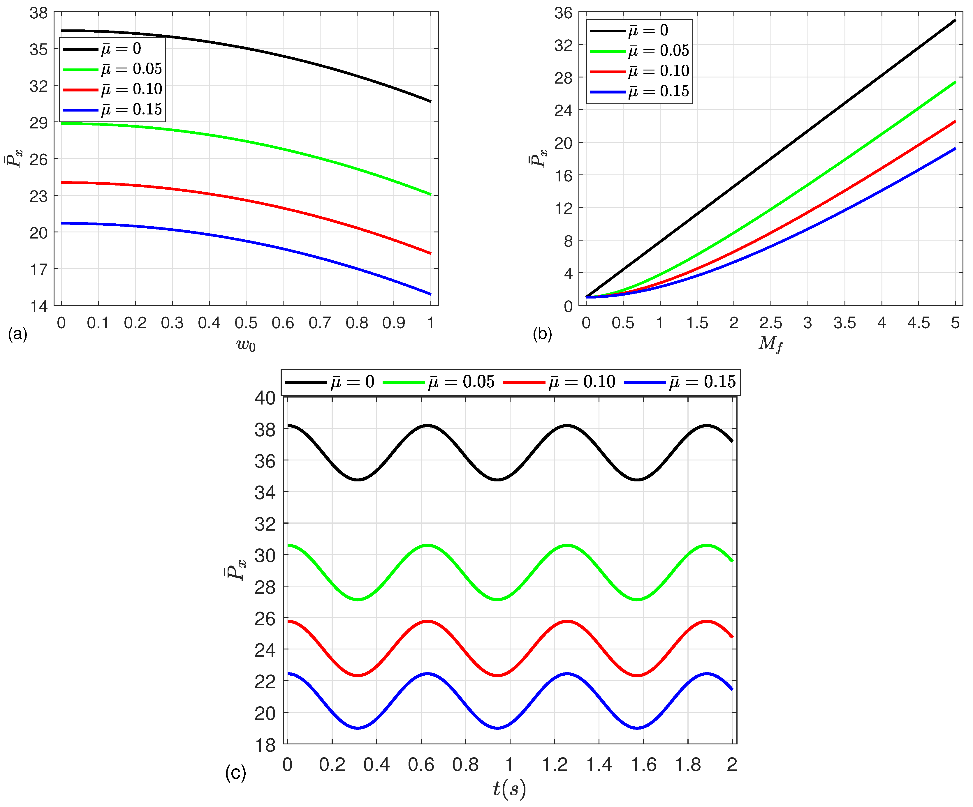
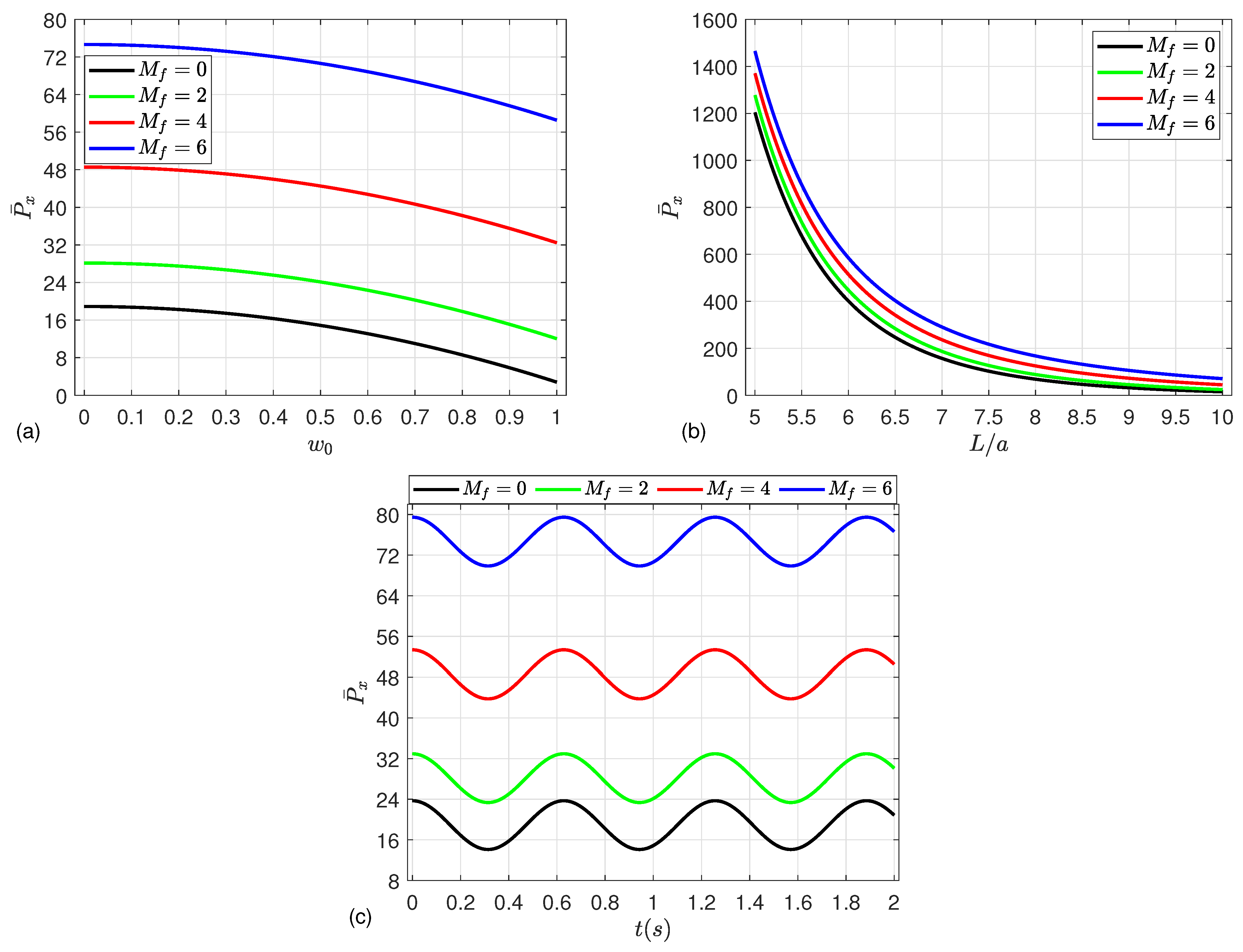
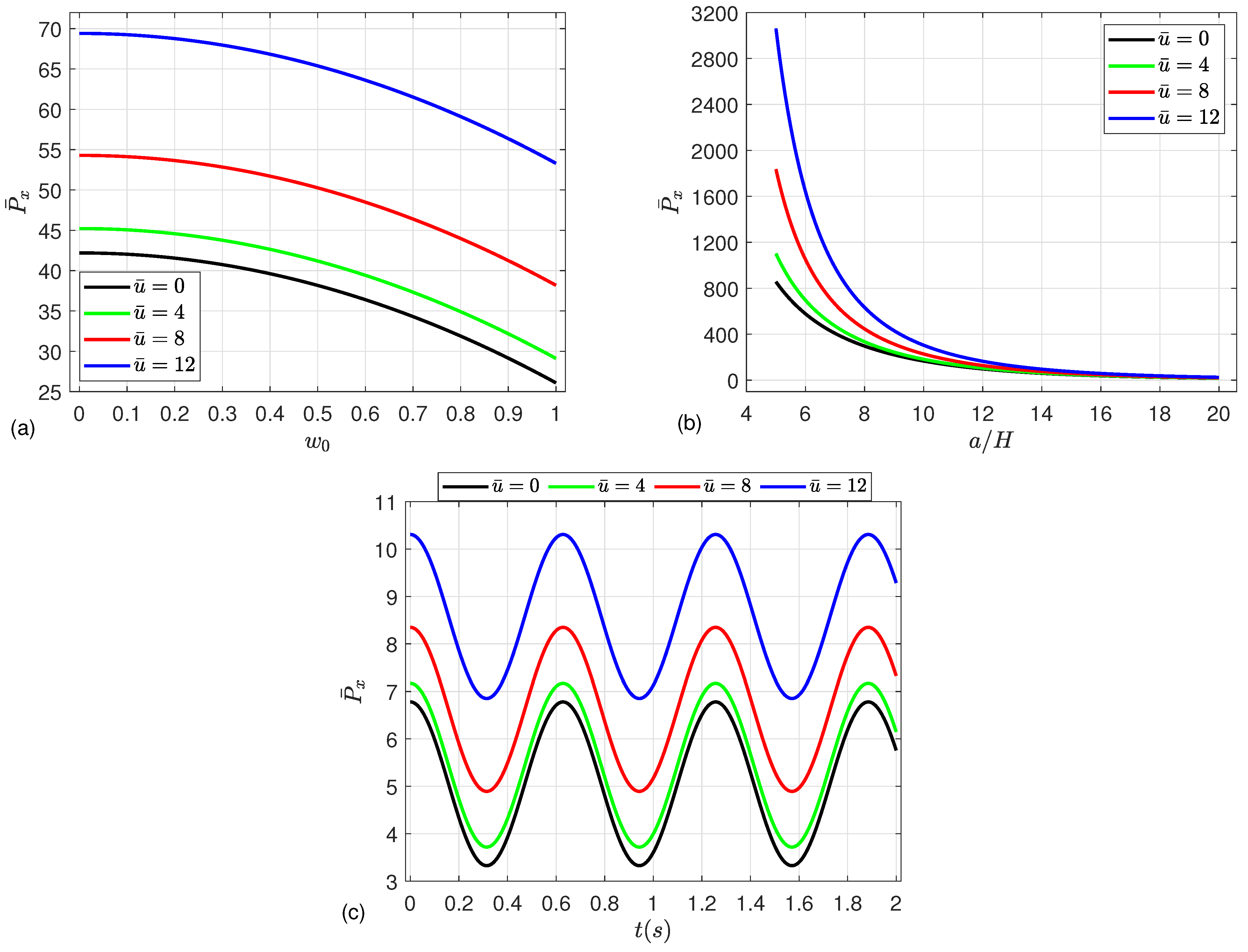
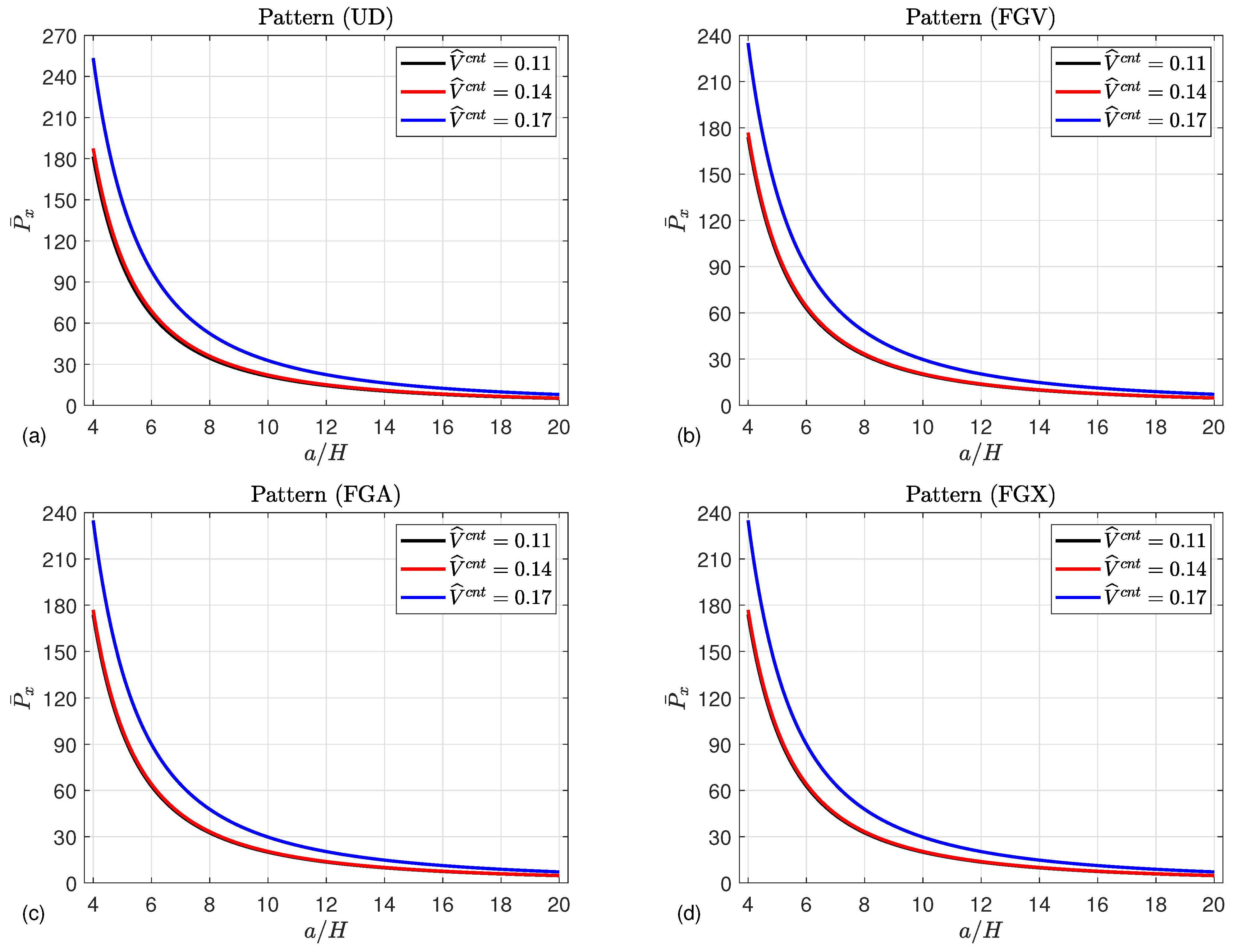
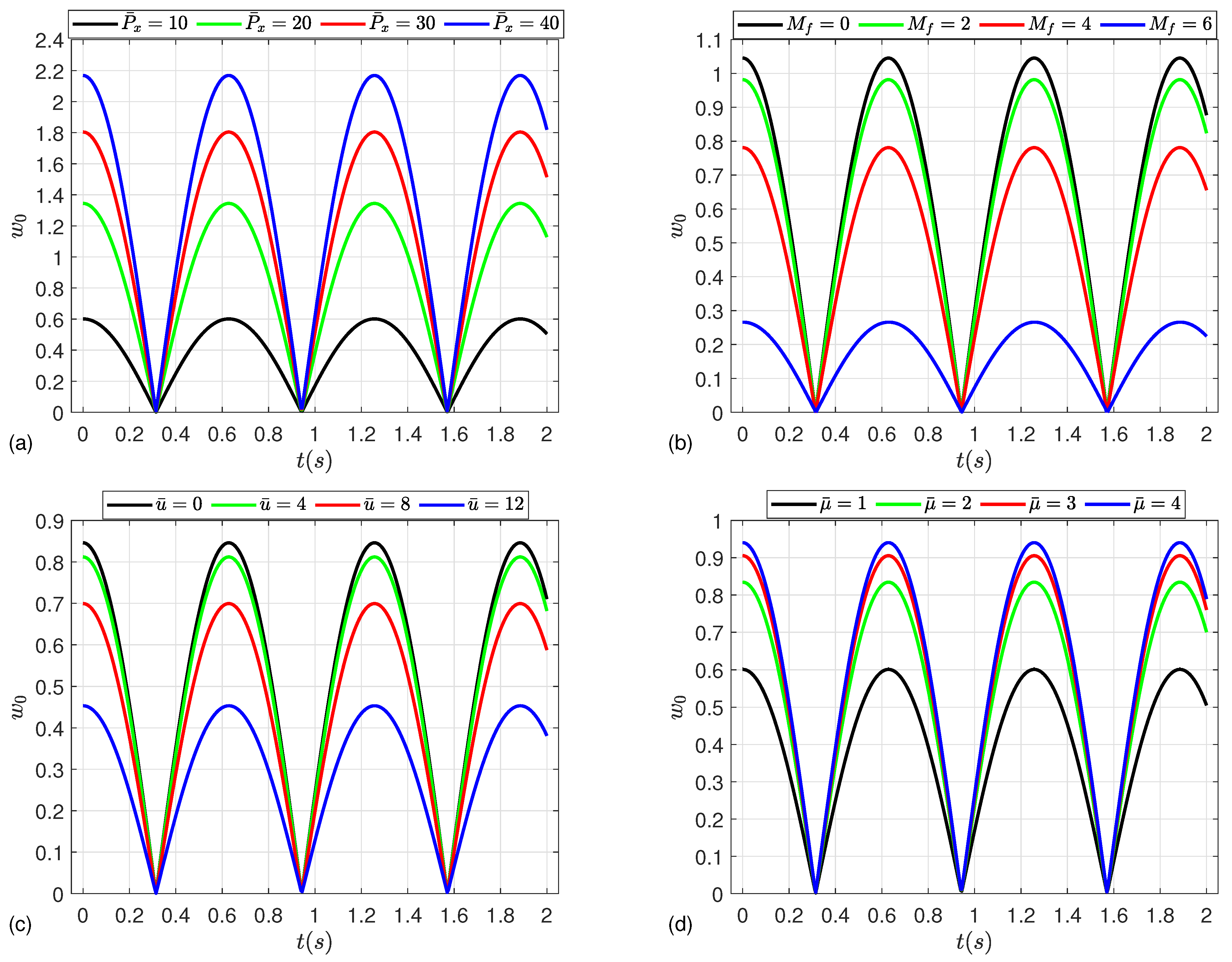
• The strength of the microshells may be enhanced by increasing the mean flow velocity, magnetic field parameter, Knudsen number, and CNT volume fraction, leading to an increment in the post-buckling paths.
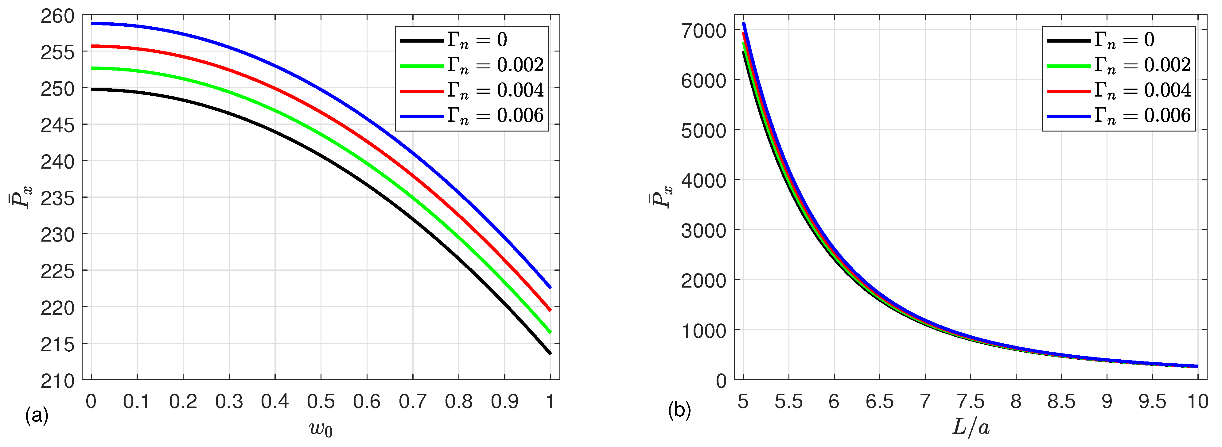
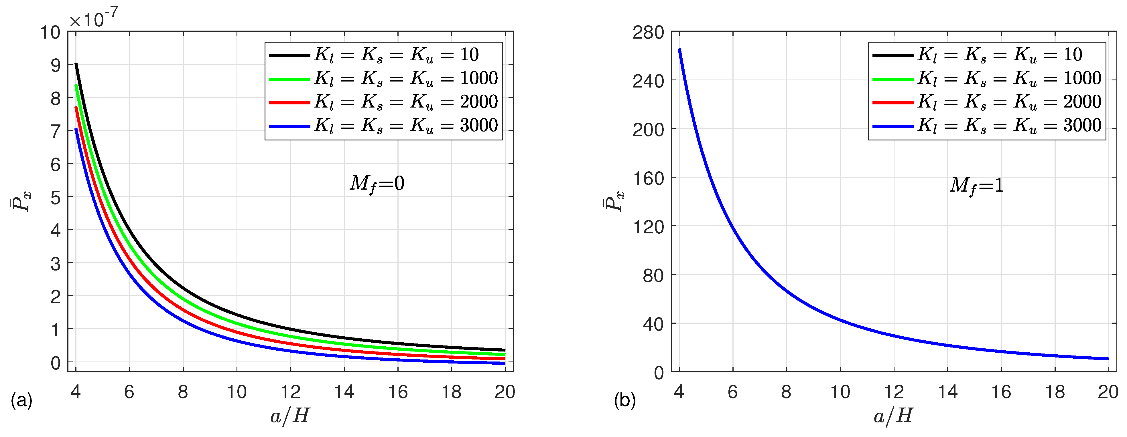
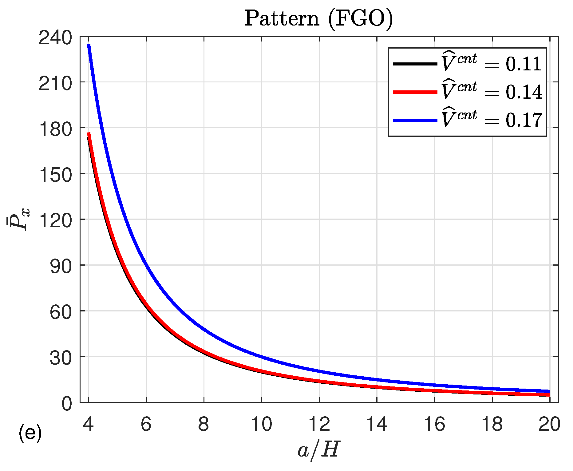
• In contrast, an increase in the radius-to-thickness ratio, length-to-radius ratio, deflection, material length scale parameter, and Kerr foundation parameters results in a reduction in post-buckling strength.
• Moreover, the nonlinear dynamic deflection increases as the compressive load and material parameter increase, while a severe reduction in the deflection occurs by increasing the magnetic parameter and mean flow velocity.
• In the absence of the magnetic field, the material length scale parameter and Kerr foundation have no influence on the post-buckling behavior.
• The theoretical insights developed here have potential applications in the design of microscale systems, including MEMS/NEMS devices, flexible microfluidic pipelines, and biomedical microtubes, where understanding the combined effects of mechanical, fluidic, and magnetic loading is critical for optimizing performance and ensuring structural stability.

References

1. Hoseinzadeh, M.; Pilafkan, R.; Maleki, V.A. Size-dependent linear and nonlinear vibration of functionally graded CNT reinforced imperfect microplates submerged in fluid medium. Ocean. Eng. 2023, 268, 113257. [Google Scholar] [CrossRef]
2. Coleman, J.N.; Khan, U.; Blau, W.J.; Gun’ko, Y.K. Small but strong: A review of the mechanical properties of carbon nanotube–polymer composites. Carbon 2006, 44, 1624–1652. [Google Scholar] [CrossRef]
3. Sun, Y.; Sun, J.; Liu, M.; Chen, Q. Mechanical strength of carbon nanotube–nickel nanocomposites. Nanotechnology 2007, 18, 505704. [Google Scholar] [CrossRef]
4. Zhu, P.; Lei, Z.; Liew, K.M. Static and free vibration analyses of carbon nanotube-reinforced composite plates using finite element method with first order shear deformation plate theory. Compos. Struct. 2012, 94, 1450–1460. [Google Scholar] [CrossRef]
5. Alibeigloo, A. Three-dimensional thermoelasticity solution of functionally graded carbon nanotube reinforced composite plate embedded in piezoelectric sensor and actuator layers. Compos. Struct. 2014, 118, 482–495. [Google Scholar] [CrossRef]
6. Sobhy, M.; Radwan, A.F. Influence of a 2D magnetic field on hygrothermal bending of sandwich CNTs-reinforced microplates with viscoelastic core embedded in a viscoelastic medium. Acta Mech. 2020, 231, 71–99. [Google Scholar] [CrossRef]
7. Radwan, A.F.; Sobhy, M. Transient instability analysis of viscoelastic sandwich CNTs-reinforced microplates exposed to 2D magnetic field and hygrothermal conditions. Compos. Struct. 2020, 245, 112349. [Google Scholar] [CrossRef]
8. Sobhy, M.; Zenkour, A.M. Magnetic field effect on thermomechanical buckling and vibration of viscoelastic sandwich nanobeams with CNT reinforced face sheets on a viscoelastic substrate. Compos. Part B Eng. 2018, 154, 492–506. [Google Scholar] [CrossRef]
9. Ghasemi, H.; Mohammadi, Y.; Ebrahimi, F. Free vibration analysis of FG-GPL and FG-CNT hybrid laminated nano composite truncated conical shells using systematic differential quadrature method. Zamm-J. Appl. Math. Mech. 2023, 103, e202300280. [Google Scholar] [CrossRef]
10. Zhao, L.C.; Xu, L.; Zeng, H.t. Thermal buckling of temperature-dependent FG-CNT reinforced composite conical-conical joined shell using GDQ. Thin-Walled Struct. 2024, 205, 112320. [Google Scholar] [CrossRef]
11. You, Q.; Hua, F.; Huang, Q.; Zhou, X. Efficient analysis on buckling of FG-CNT reinforced composite joined conical–cylindrical laminated shells based on GDQ method under multiple loading conditions. Mech. Adv. Mater. Struct. 2024, 31, 11173–11190. [Google Scholar] [CrossRef]
12. Sobhani, E.; Safaei, B. Vibrational characteristics of attached hemispherical-cylindrical ocean shell-structure reinforced by CNT nanocomposite with graded pores on two-parameter elastic foundations applicable in offshore components. Ocean. Eng. 2023, 285, 115413. [Google Scholar] [CrossRef]
13. Avey, M.; Fantuzzi, N.; Sofiyev, A. Mathematical modeling and analytical solution of thermoelastic stability problem of functionally graded nanocomposite cylinders within different theories. Mathematics 2022, 10, 1081. [Google Scholar] [CrossRef]
14. Nguyen, T.N.; Dang, L.M.; Lee, J.; Nguyen, P.V. Load-carrying capacity of ultra-thin shells with and without CNTs reinforcement. Mathematics 2022, 10, 1481. [Google Scholar] [CrossRef]
15. Chang, X.; Hong, X.; Qu, C.; Li, Y. Stability and nonlinear vibration of carbon nanotubes-reinforced composite pipes conveying fluid. Ocean. Eng. 2023, 281, 114960. [Google Scholar] [CrossRef]
16. Mahesh, V.; Harursampath, D. Nonlinear vibration of functionally graded magneto-electro-elastic higher order plates reinforced by CNTs using FEM. Eng. Comput. 2022, 38, 1029–1051. [Google Scholar] [CrossRef]
17. Sheng, G.; Han, Y.; Zhang, Z.; Zhao, L. Nonlinear dynamic response of functionally graded cylindrical microshells conveying steady viscous fluid. Compos. Struct. 2021, 274, 114318. [Google Scholar] [CrossRef]
18. Kerschan-Schindl, K.; Grampp, S.; Henk, C.; Resch, H.; Preisinger, E.; Fialka-Moser, V.; Imhof, H. Whole-body vibration exercise leads to alterations in muscle blood volume. Clin. Physiol. 2001, 21, 377–382. [Google Scholar] [CrossRef]
19. Ashley, H.; Haviland, G. Bending vibrations of a pipe line containing flowing fluid. J. Appl. Mech. 1950, 17, 229–232. [Google Scholar] [CrossRef]
20. Weaver, D.; Ziada, S.; Au-Yang, M.; Chen, S.; Paı, M. Flow-induced vibrations in power and process plant components-progress and prospects. J. Press. Vessel. Technol. 2000, 122, 339–348. [Google Scholar] [CrossRef]
21. Webster, P.M.; Sawatzky, R.P.; Hoffstein, V.; Leblanc, R.; Hinchey, M.J.; Sullivan, P.A. Wall motion in expiratory flow limitation: Choke and flutter. J. Appl. Physiol. 1985, 59, 1304–1312. [Google Scholar] [CrossRef] [PubMed]
22. Firouz-Abadi, R.; Noorian, M.; Haddadpour, H. A fluid–structure interaction model for stability analysis of shells conveying fluid. J. Fluids Struct. 2010, 26, 747–763. [Google Scholar] [CrossRef]
23. Zhang, D.; Li, P.; Lu, J.; Zhang, C.; Yang, Y. Stability analysis of cylindrical shell in axial flow: A DQ-based approach and an instability prediction formula. Ocean. Eng. 2023, 267, 113198. [Google Scholar] [CrossRef]
24. Ma, Y.; Wang, Z.M. Vibration Characteristics of a Functionally Graded Viscoelastic Fluid-Conveying Pipe with Initial Geometric Defects under Thermal–Magnetic Coupling Fields. Mathematics 2024, 12, 840. [Google Scholar] [CrossRef]
25. Zhang, Y.L.; Reese, J.M.; Gorman, D.G. Finite element analysis of the vibratory characteristics of cylindrical shells conveying fluid. Comput. Methods Appl. Mech. Eng. 2002, 191, 5207–5231. [Google Scholar] [CrossRef]
26. Paak, M.; Païdoussis, M.; Misra, A. Nonlinear dynamics and stability of cantilevered circular cylindrical shells conveying fluid. J. Sound Vib. 2013, 332, 3474–3498. [Google Scholar] [CrossRef]
27. Mohammadimehr, M.; Mehrabi, M. Stability and free vibration analyses of double-bonded micro composite sandwich cylindrical shells conveying fluid flow. Appl. Math. Model. 2017, 47, 685–709. [Google Scholar] [CrossRef]
28. Rashvand, K.; Alibeigloo, A.; Safarpour, M. Free vibration and instability analysis of a viscoelastic micro-shell conveying viscous fluid based on modified couple stress theory in thermal environment. Mech. Based Des. Struct. Mach. 2022, 50, 1198–1236. [Google Scholar] [CrossRef]
29. Ebrahimi, Z. Free vibration and stability analysis of a functionally graded cylindrical shell embedded in piezoelectric layers conveying fluid flow. J. Vib. Control. 2023, 29, 2515–2527. [Google Scholar] [CrossRef]
30. Abdollahi, R.; Firouz-Abadi, R.; Rahmanian, M. Nonlinear vibrations and stability of rotating cylindrical shells conveying annular fluid medium. Thin-Walled Struct. 2022, 171, 108714. [Google Scholar] [CrossRef]
31. Al-Furjan, M.S.H.; Bolandi, S.Y.; Habibi, M.; Ebrahimi, F.; Chen, G.; Safarpour, H. Enhancing vibration performance of a spinning smart nanocomposite reinforced microstructure conveying fluid flow. Eng. Comput. 2022, 38, 4097–4112. [Google Scholar] [CrossRef]
32. Hoang, V.N.V.; Thanh, P.T.; Toledo, L. Impact of non-homogeneous Winkler–Pasternak foundation on nonlinear dynamic characteristics of fluid-conveying functionally graded cylindrical shells. Ocean. Eng. 2024, 307, 118123. [Google Scholar] [CrossRef]
33. Sobhy, M. Nonlinear deflection and traveling wave solution for FG-GPLs reinforced microtubes embedded in Kerr foundation and conveying magnetic fluid. Ocean. Eng. 2024, 296, 117026. [Google Scholar] [CrossRef]
34. Zhang, J.; Zhang, W.; Zhang, Y. Nonlinear resonant analyses of graphene oxide powder reinforced hyperelastic cylindrical shells containing flowing-fluid. Thin-Walled Struct. 2024, 203, 112248. [Google Scholar] [CrossRef]
35. Johari, V.; Hassani, A.; Talebitooti, R.; Kazemian, M. Free vibration analysis of a circular cylindrical shell using a new four-variable refined shell theory. Proc. Inst. Mech. Eng. Part J. Mech. Eng. Sci. 2022, 236, 7079–7094. [Google Scholar] [CrossRef]
36. Sobhy, M.; Radwan, A.F. Porosity and size effects on electro-hygrothermal bending of FG sandwich piezoelectric cylindrical shells with porous core via a four-variable shell theory. Case Stud. Therm. Eng. 2023, 45, 102934. [Google Scholar] [CrossRef]
37. Ma, H.; Gao, X.L.; Reddy, J. A microstructure-dependent Timoshenko beam model based on a modified couple stress theory. J. Mech. Phys. Solids 2008, 56, 3379–3391. [Google Scholar] [CrossRef]
38. Yang, F.; Chong, A.; Lam, D.C.C.; Tong, P. Couple stress based strain gradient theory for elasticity. Int. J. Solids Struct. 2002, 39, 2731–2743. [Google Scholar] [CrossRef]
39. Esawi, A.M.; Farag, M.M. Carbon nanotube reinforced composites: Potential and current challenges. Mater. Des. 2007, 28, 2394–2401. [Google Scholar] [CrossRef]
40. Fidelus, J.; Wiesel, E.; Gojny, F.; Schulte, K.; Wagner, H. Thermo-mechanical properties of randomly oriented carbon/epoxy nanocomposites. Compos. Part Appl. Sci. Manuf. 2005, 36, 1555–1561. [Google Scholar] [CrossRef]
41. Shen, H.S. Nonlinear bending of functionally graded carbon nanotube-reinforced composite plates in thermal environments. Compos. Struct. 2009, 91, 9–19. [Google Scholar] [CrossRef]
42. Song, Z.; Zhang, L.; Liew, K. Vibration analysis of CNT-reinforced functionally graded composite cylindrical shells in thermal environments. Int. J. Mech. Sci. 2016, 115, 339–347. [Google Scholar] [CrossRef]
43. Sobhy, M. Levy solution for bending response of FG carbon nanotube reinforced plates under uniform, linear, sinusoidal and exponential distributed loadings. Eng. Struct. 2019, 182, 198–212. [Google Scholar] [CrossRef]
44. John, K. Electromagnetics; McGraw-Hill: New York, NY, USA, 1984. [Google Scholar]
45. Sobhy, M.; Al Mukahal, F.H. Magnetic control of vibrational behavior of smart FG sandwich plates with honeycomb core via a quasi-3D plate theory. Adv. Eng. Mater. 2023, 25, 2300096. [Google Scholar] [CrossRef]
46. Sobhy, M. 3-D elasticity numerical solution for magneto-hygrothermal bending of FG graphene/metal circular and annular plates on an elastic medium. Eur. J.-Mech.-A/Solids 2021, 88, 104265. [Google Scholar] [CrossRef]
47. Sadeghi-Goughari, M.; Jeon, S.; Kwon, H.J. Effects of magnetic-fluid flow on structural instability of a carbon nanotube conveying nanoflow under a longitudinal magnetic field. Phys. Lett. A 2017, 381, 2898–2905. [Google Scholar] [CrossRef]
48. Andersson, H. An exact solution of the Navier-Stokes equations for magnetohydrodynamic flow. Acta Mech. 1995, 113, 241–244. [Google Scholar] [CrossRef]
49. Wang, L.; Ni, Q. A reappraisal of the computational modelling of carbon nanotubes conveying viscous fluid. Mech. Res. Commun. 2009, 36, 833–837. [Google Scholar] [CrossRef]
50. Rashidi, V.; Mirdamadi, H.R.; Shirani, E. A novel model for vibrations of nanotubes conveying nanoflow. Comput. Mater. Sci. 2012, 51, 347–352. [Google Scholar] [CrossRef]
51. Mirramezani, M.; Mirdamadi, H.R. Effects of nonlocal elasticity and Knudsen number on fluid–structure interaction in carbon nanotube conveying fluid. Phys.-Low-Dimens. Syst. Nanostruct. 2012, 44, 2005–2015. [Google Scholar] [CrossRef]
52. Sobhy, M.; Radwan, A.F. Levy solution and state-space approach for hygro-thermo-magnetic bending of a cross-ply laminated plate on Kerr foundation under various loadings. J. Compos. Mater. 2025, 59, 3–28. [Google Scholar] [CrossRef]
53. Han, Y.; Elliott, J. Molecular dynamics simulations of the elastic properties of polymer/carbon nanotube composites. Comput. Mater. Sci. 2007, 39, 315–323. [Google Scholar] [CrossRef]
54. Khdeir, A.; Reddy, J.; Frederick, D. A study of bending, vibration and buckling of cross-ply circular cylindrical shells with various shell theories. Int. J. Eng. Sci. 1989, 27, 1337–1351. [Google Scholar] [CrossRef]
Figure 1. Schematic of the system considered.
Mathematics 13 01518 g001
Figure 2. An FG-CNTs reinforced microshell integrated with Kerr foundation.
Mathematics 13 01518 g002
Figure 3. Schematic diagrams of five types of CNT distribution.
Mathematics 13 01518 g003
Figure 4. Post-buckling behavior of microfluid-conveying UD-CNTs cylindrical microshells with the variation of (a) the maximum deflection w 0 , (b) magnetic field parameter M f , and (c) time t for different values of the material length scale parameter μ ¯ ( t = 1 s).
Mathematics 13 01518 g004
Figure 5. Post-buckling behavior of microfluid-conveying UD-CNTs cylindrical microshells with the variation of (a) the maximum deflection w 0 , (b) length-to-radius ratio L / a , and (c) time t for different values of the magnetic field parameter M f ( t = 1 s, a / H = 15 ).
Mathematics 13 01518 g005
Figure 6. Post-buckling behavior of microfluid-conveying UD-CNTs cylindrical microshells with the variation of (a) the maximum deflection w 0 , (b) radius-to-thickness ratio a / H , and (c) time t for different values of the mean flow velocity u ¯ ( t = 1 s, a / H = 15 ).
Mathematics 13 01518 g006
Figure 7. Post-buckling behavior of microfluid-conveying UD-CNTs cylindrical microshells with the variation of (a) the maximum deflection w 0 and (b) length-to-radius ratio L / a for different values of the Knudsen number Γ ( a / H = 10 ) ( t = 1 s).
Mathematics 13 01518 g007
Figure 8. Post-buckling behavior of UD-CNTs cylindrical shells with the variation of the radius-to-thickness ratio a / H for different values of the Kerr foundation parameters K l , K s , and K u (a) without magnetic field ( M f = 0 ) and (b) with magnetic field ( M f = 1 ) ( μ ¯ = u ¯ = 0 , w 0 = 0.00005 ).
Mathematics 13 01518 g008
Figure 9. Post-buckling behavior of microfluid-conveying cylindrical microshells with various CNT distributions (a) UD, (b) FGV, (c) FGA, (d) FGX, and (e) FGO for different values of the CNT volume fraction V ^ c n t ( L / a = 20 , M f = 0 , w 0 = 0.4 ).
Mathematics 13 01518 g009aMathematics 13 01518 g009b
Figure 10. Nonlinear time response of the maximum deflection of microfluid-conveying UD-CNT cylindrical microshells for different values of (a) the axial compressive load P ¯ x , (b) the magnetic field parameter M f , (c) the mean flow velocity u ¯ , and (d) the material length scale parameter μ ¯ .
Mathematics 13 01518 g010