1. Introduction
In the context of the 5G trend spreading globally, a series of digital technologies represented by blockchain, cloud computing, mobile Internet, artificial intelligence, and large language models are gradually infiltrating the field of financial technology. Digital technology and inclusive finance present a new mode of accelerating deep integration, and the concept of digital inclusive finance is widely acknowledged in various countries [
1]. Nowadays, many countries are exploring the possibility of digital inclusive finance being widely used in various fields: China is fully exploiting the digital use of Internet banks [
2] and uses blockchain’s de-trusting and smart contract mechanism to break the vertical development barriers of inclusive finance [
3] to create a digital inclusive finance value chain. Nigeria has leveraged its massive emerging market to join forces with Mobile Money Operators (MMOs) to actively promote the path to digital inclusive finance [
4]. France is looking at the relationship between inclusive finance and poverty to explore a sustainable and inclusive economic model [
5].
In their studies, scholars in various countries have found that weak economic performance, persistently high invisible and cyclical unemployment rates [
6], and constraints in economic policies implemented in some regions [
7] keep emerging due to the low utilization of labor resources in rural areas. In addition, there is a low degree of openness in the rural financial system, with a dysfunctional economy, a single source of financing, and a high degree of financial exclusion. The emergence of a trend in digital financial activities has led to significant structural changes in the agricultural economy, but the marginal contribution of digital inclusive finance to the development of rural labor economics (RLE) is relatively greater. At the same time, RLE is the most widespread individual beneficiary based on the social significance of its concept of “inclusion” and its ability to provide more services to vulnerable groups [
8]. The development of labor economics not only affects rural economic development and farmers’ income growth but also has a significant impact on human and social development in rural areas [
9]. Therefore, studying the intrinsic impact of digital inclusive finance on RLE makes an important theoretical contribution and has application value. It is from an inclusive perspective that this paper discusses the inclusive value of digital finance and its role in the economic development of rural areas. It also provides a deeper understanding of the behavioral logic of rural residents, who are a vulnerable group in the financial market, in harnessing the inclusive value of digital financial innovation to seek their own financial development.
In recent years, along with the gradual penetration of digital technologies represented by 5G and the Internet of Things into traditional rural economics and the continuous innovation and integration development, digital inclusive finance is establishing a multilevel and wide coverage service system in rural areas. At the same time, RLE also shows an increasingly diversified development trend [
10]. To further explore the depth and convenience of its use in the development process, scholars from various countries have explored the multidimensional impacts of the technologies and services covered by digital inclusive finance from different perspectives concerning their widespread application in RLE. From a macroscopic perspective, the introduction of the overall concept of digital inclusive finance and the use of a series of digital technologies included in it have effectively contributed to the innovative development and systemic improvement of RLE. In terms of its innovation to develop RLE, Luo and Wang [
11] conducted an empirical study on Chinese household tracking survey data. It was found that increasing investment in digital infrastructure while integrating digital technologies represented by blockchain, cloud computing, artificial intelligence, and the Internet of Things with traditional rural industries can give rise to a series of innovative business models and modes such as distance education, online healthcare, and platform economy. This will reshape the competitive advantage of RLE. Du et al. [
12] analyzed inter-provincial panel data in China for the last decade using a panel threshold effect and a mediating effect model. It is found that there is a double threshold effect of the breadth of digital inclusive financial coverage and the degree of digitalization on the upgrading of the consumption structure of rural residents, which mainly shows a “marginal increasing” and “inverted S-shaped” nonlinear pattern. The construction of digital inclusive finance infrastructure in rural areas can effectively promote the structural upgrading of RLE. By studying the impact of digitalization on agribusiness activity, Davydchuk [
13] found that digitalization has become the essence of modern mechanisms for managing enterprises’ financial and economic activities in rural areas. It effectively increases the level of technological development of production and management activities, as well as the competitiveness of rural enterprises. As for the improvement and optimization of the RLE system, Murendo et al. [
14] used Poisson and negative binomial regression to assess the relationship between inclusive finance and the nutrition of rural households in the Zimbabwean region. Using digital finance as a factor of socioeconomic stability in rural areas, it was found that the promotion of digital inclusive financial services among rural and poor households was effective in reducing information inequality and transaction costs among urban and rural residents. Sup et al. [
15] discuss the methodology of regional agribusiness development strategies, using digital economy elements to establish priority principles of development management in the field of regional agribusiness, and implementing management systems in the digital economy information space. This contributes to the process of modernization of management systems for the development of the labor economy in subsectors and rural areas.
At the micro level, the core competencies that specific technologies can bring to RLE are analyzed from a range of digital technologies that make up digital inclusive finance. Thakur and Prasad [
16] compare the differences between communication infrastructure and population ratios in developed and developing countries while examining successful implementation cases in the state of Jharkhand. They found that the wide coverage of 5G technology in rural areas can bridge the huge digital divide between rural and urban areas, allowing for efficient and flexible information technology transmission and communication. Qinya et al. [
17] discussed the development opportunities of the agricultural economy and rural tourism under big data, based on the important position of the agricultural economy in China’s national economy and the connotation and characteristics of big data, and concluded that combining rural economic reform with big data technology can improve the overall quality of rural economic development. The conclusion was that combining rural economic reform with big data technology can improve the overall quality of rural economic development. Nyika [
18] compares the extent of Information and Communication Technology (ICT) adoption in different areas and explores the factors that impede ICT-driven socioeconomic development in developing countries and rural areas, finding that maximizing the potential benefits of marginalized communities can enable rural areas to benefit from limited ICT for transformative development in a variety of areas, including agriculture, education, medicine, tourism, and business. Dai and Min [
19] introduced blockchain technology into the overall scenario of RLE to decipher order-based agricultural financing. They focus on introducing guarantee functions such as comprehensive financing credit and risk retransfers into the specific aspects of order signing and pledge loans, thus building a financing mechanism for rural economies with the synergy of multiple entities. Guneo [
20] looks at the effects on savings of mobile money in rural Kenya. A cross-sectional household survey and net effect analysis revealed that technological innovations in mobile money and rotating savings, and the development of formal financial service institutions such as rotating savings and credit cooperatives were effective in alleviating the constraints on the development of RLE due to the inadequacy of the local financial system. Zhang [
21] fully explored the diverse financial management models of collective economic organizations in rural areas. It was found that artificial intelligence technology can build an integrated financial and business management platform by strengthening the initiative of managers and expanding the management accounting business. This brings extensive changes to the financial management of RLE. Ma et al. [
22] used endogenous treatment regression and unconditional quantile regression techniques to identify the effects of homogeneity and heterogeneity on Internet use. The widespread use of Internet technology in rural areas was found to have a profound impact on the higher distribution of household income and expenditure. Briglauer [
23] used a matched difference-in-difference estimation strategy to analyze the impact of a speedup in broadband Internet availability applied to rural areas in Bavaria, Germany, in a European state aid program. He found that increased broadband coverage by local governments through state aid had a positive effect on the economic development and employment rates of residents in rural areas.
The majority of previous studies have examined the benefits of digital inclusive finance in terms of its impact on RLE development from the perspectives of macroeconomic conditions and micro market structures. Among them, methods such as panel thresholds, mesomeric effects, and negative binomial regressions have been applied in empirical studies on the impact mechanisms of digital inclusive finance to assess the overall impact that digital inclusive finance has on the economy of rural areas. Simultaneously, some studies have tapped into the economic benefits generated in rural areas from the perspective of specific digital technologies such as communication infrastructure, integrated commodity trading systems, blockchain, and mobile money. However, theoretically speaking, the majority of previous research has only explored a particular aspect of the content of RLE development in the context of digital finance. They lack a comprehensive framework integrating the multidimensional impact mechanisms between digital inclusive finance and RLE. On the empirical side, further supplementation is needed for scientific and standardized quantitative verification and empirical data analysis.
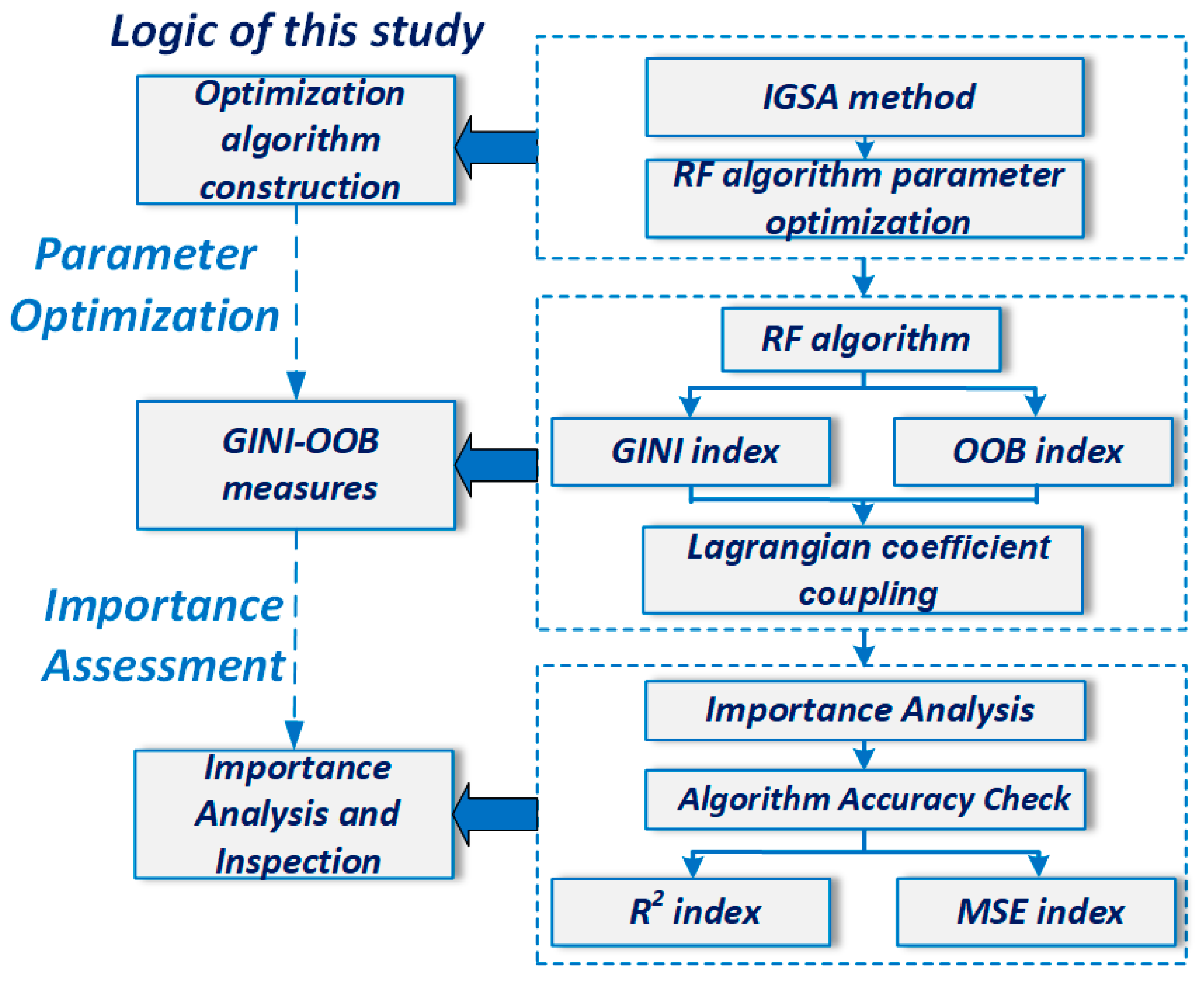
As the application of machine learning in the financial market continues to expand, the use of machine learning, deep learning, and data mining algorithms in risk management and portfolio optimization has achieved remarkable success. However, limited research has been conducted on leveraging machine learning algorithms, such as the Improved Gravitational Search Algorithm-Random Forest (IGSA-RF), to analyze the connection between digital inclusive finance and RLE. Therefore, this paper aims to construct a RLE indicator system using IGSA-RF and assess the impact of digital inclusive finance on each indicator based on the Gini-Out-of-Bag (Gini-OOB) coupling perspective.
As machine learning continues to expand its role in financial applications such as risk management and portfolio optimization [
24], Random Forest (RF), a widely adopted ensemble learning algorithm, has demonstrated strong robustness through Bootstrap aggregation and its ability to estimate feature importance. Recent extensions, such as the concept drift-handling RF variant proposed by Zhukov et al. [
25], further enhance its adaptability to dynamic environments. However, limited research has explored the integration of machine learning models like RF with rural economic systems. To address this gap, this paper constructs a rural labor economics (RLE) indicator system using an Improved Gravitational Search Algorithm-Random Forest (IGSA-RF) model and evaluates the influence of digital inclusive finance through a Gini-Out-of-Bag (Gini-OOB) coupling perspective.
Firstly, we review relevant literature and establish a multidimensional RLE indicator system. To enhance feature selection and improve model accuracy, we propose an Improved Gravitational Search Algorithm, which optimizes the conventional Gravitational Search Algorithm from three dimensions. This optimized algorithm is integrated into Random Forest to refine parameter selection and feature importance evaluation. To highlight the key indicators and further quantify their impact, we employ the minimum relative information entropy principle to construct the Gini-OOB coupling coefficient. Additionally, we utilize the Lagrange multiplier method to optimize the calculation formula for combination weights. IGSA-RF ensures strong adaptability and self-learning capability, making the model construction process more robust and scientifically sound. Finally, we validate the rationality and effectiveness of the model through empirical analysis.
This paper is organized as follows:
Section 2 reviews RLE and digital inclusive finance in the context of the literature, and
Section 3 presents the methodology and indicator tests used to construct the RLE index model;
Section 4 performs data processing and specific empirical analysis;
Section 5 presents the experimental results and evaluates the validity of the model, giving a sound opinion; this is followed by the conclusion in
Section 6.
3. Methodology
This paper proposes a robust IGSA-RF algorithm-based method for identifying feature importance in rural labor economic indicators from a Gini-OOB dual perspective. To measure the impact of digital inclusive finance on each indicator, the Gini-OOB coupling coefficient is constructed. Firstly, we introduce the GSA and optimize it from three dimensions, leading to the development of IGSA for enhanced parameter tuning of RF. Next, the IGSA-RF algorithm is applied to select the most relevant features during splitting [
68], traversing all tree nodes and calculating the split impurity
for all variables. Then, we use RF samples to autonomously train and generate a self-help sample set [
69], perturb the Out-of-Bag data of the features, and use the quantified error rate to measure the replacement importance
of the variables. Finally, we employ the minimum relative information entropy principle and apply the Lagrange multiplier method to integrate
and
, constructing the Gini-OOB coupling coefficient to assess the degree of influence of digital inclusive finance on various indicators of RLE. The methodology framework is illustrated in
Figure 3.
3.1. Nomenclature
To facilitate clarity and consistency in the presentation of the proposed methodology, the key mathematical symbols, variables, and function spaces used throughout this section are defined and summarized in
Table 3.
3.2. The IGSA Method
While meta-heuristic optimizers such as Particle Swarm Optimization (PSO) and Genetic Algorithm (GA) are widely used for tuning machine learning models, they often exhibit premature convergence and can stall in local optima due to limited exploration–exploitation balance. PSO may converge too quickly around suboptimal regions, and GA’s crossover/mutation operations can be computationally expensive when searching high-dimensional spaces. By contrast, the Gravitational Search Algorithm (GSA) leverages a chaotic perturbation operator and an adaptive gravitational constant to maintain diverse agent interactions, thereby reducing the risk of local trapping and improving convergence speed [
70,
71]. This study enhances the GSA from three dimensions, developing an IGSA to optimize key parameters in the RF model. Specifically, IGSA is used to fine-tune the number of decision trees, the maximum number of features selected at each split, and the minimum sample split, ensuring optimal parameter selection and improving model robustness.
In IGSA, agents represent mass-bearing objects exerting attractive forces on one another, with greater masses generating stronger attraction. The agent with the highest mass is assumed to hold the optimal position. Given
N agents in a
d-dimensional space, the position of the
i-th agent is defined as follows:
At the
t-th iteration, the force on the
i-th agent from the
j-th agent is given by
where
and
are the masses of agents
i-th and
j-th agent.
G(t) is the gravitational constant at time,
is a small constant, and
is the Euclidean distance between the
i-th agent and the
j-th agent. The total force on the
i-th agent is
where
rand is a uniform random variable between [0, 1]. The acceleration of the agent at time
t is
The velocity and position of the
i-th agent are updated as
where
and
are the current position and velocity of the agent. While the conventional GSA works well for parameter optimization in RF, its updates of gravitational coefficients and iteration speeds are relatively slow [
70]. To overcome these limitations, we propose IGSA, which enhances the gravitational coefficient, update speed formula, and position update formula.
where
randi,
randj, and
randk are random variables in the interval [0, 1];
c1,
c2 are constants in [0, 1];
is the best position of particle
i; and
is the best position of all particles. By adjusting
c1 and
c2, the balance between gravity, memory, and population information can be controlled.
Position update. The differential evolution algorithm uses a greedy selection mode, as shown in Equation (10). If the fitness value of the new individual surpasses the target individual, it is accepted; otherwise, the previous generation’s individual remains in the population. The new position’s fitness is lower than the target’s.
3.3. The RF Method
Random Forest, a supervised learning algorithm based on Bagging as a logical basis, is a combination of multiple decision tree classifiers {
h(
X,
),
k = 1, …}. The sets of attributes
represent the growth process of a single decision tree, which are only weakly dependent or even unrelated to each other. They are assigned the same weight and parallelized at the same time. Assuming that the independent variable
X is known, each decision tree is entitled to jointly select the final classification result. The RF algorithm is well adapted and tolerant to noise and outliers in the sample. In addition, it shows a high prediction accuracy in both classification and regression models [
72]. The basic principle of RF is as follows:
Step 1: The Bootstrap resampling method is used. Setting the original training dataset , i ∈ [1, N], m ∈ [1, M], xi represents N sample data, m represents the number of features of each sample, and k training sub-samples are randomly selected.
Step 2: Decision trees are constructed. A k-decision tree model is constructed using the k-group set, while k out-of-band data are generated.
Step 3: The optimal splitting feature is selected. At the splitting node of each decision tree,
m features are randomly drawn from
M features, and the best feature is selected as the splitting feature, with
m being constant. The complete splitting process is recorded using classifier
hj(
x) to form a Random Forest [
73]. The calculation formula of the classifier is shown in Equation (11):
where
Y is the output variable and
j denotes the
jth classifier. the Gini coefficient is generally used as a measure to determine the left and right features.
Step 4: Making decisions. Training
T times, the combined model formula is shown in Equation (12):
where
is the schematic function. The model processing flow is shown in
Figure 4.
RF has demonstrated exceptional prediction performance on numerous datasets [
68], while possessing strong noise resistance capabilities that enable it to provide feature importance rankings even when there are errors in the training data. However, RF still has some shortcomings when it comes to handling feature selection. The RF algorithm currently uses Gini importance, Information Gain, OOB error, Mean Decrease Impurity (MDI), Mean Decrease Accuracy (MDA), and node degree as the main metrics to evaluate the relative importance of the features [
74]. However, among the indicators such as Information Gain, MDI, etc., there is a tendency to characterize preferences for more values. The remaining node degree and cumulative node degree are susceptible to data dimensions, making them incompatible with high-dimensional data or requiring high saturation of the dataset. Therefore, most scholars choose to use coupled metrics associated with the Gini coefficient for training to improve model performance and the interpretability of feature importance while being compatible with data dimensions and reducing the risk of overfitting [
75].
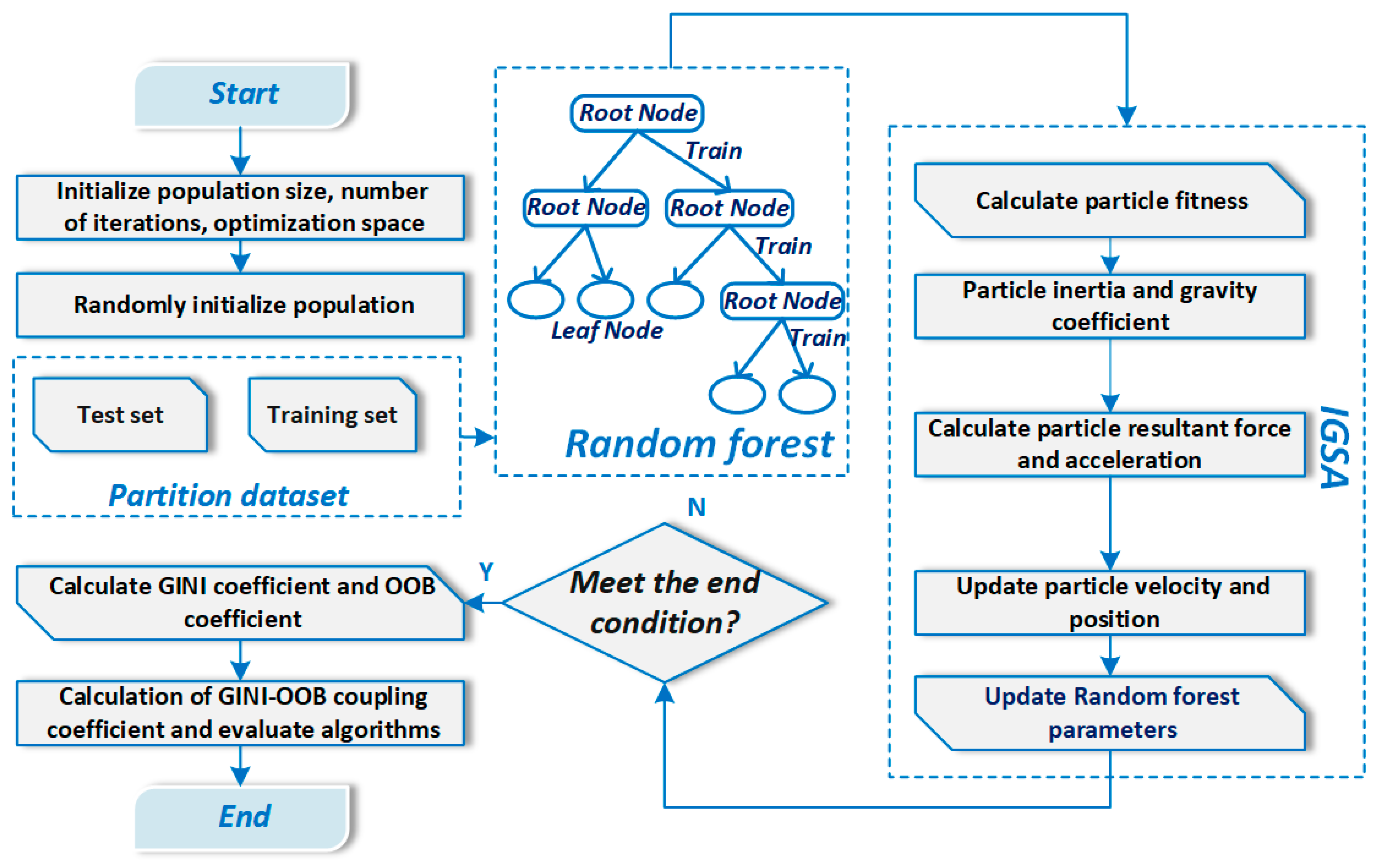
3.4. The IGSA-RF Prediction Model
In the learning process of the RF algorithm, key parameters need to be determined, such as the number of decision trees, the number of randomly selected features at each node, and the splitting criteria [
76,
77]. In the optimized prediction model of RF, these key parameters are encoded as particles in the IGSA. The optimization is performed based on the gravitational interaction between individuals until the optimal solution is found. The optimal parameters obtained from the IGSA are then used to set the number of trees, the number of features, and the splitting criteria in the RF model, resulting in the IGSA-RF prediction model [
78]. The flowchart is shown in
Figure 5. To better understand the scalability and efficiency of the proposed method, we also analyzed its computational complexity. Specifically, the time complexity of the IGSA-RF algorithm can be expressed as
where
P denotes the population size of IGSA agents,
G is the number of iterations, and
is the complexity of training a single RF model. The training cost is approximately
With representing the number of decision trees and N the number of samples. In our experiments, we used P = 30, G = 100, and = 15, making the total model training process highly efficient, with an average runtime of 3.6 s per experiment (standard deviation: 0.4 s) on a standard desktop computer (Intel Core i7, 16 GB RAM). This demonstrates the practicality and scalability of the IGSA-RF model for real-world applications.
3.5. The GINI-OOB Coefficient
3.5.1. The GINI Coefficient
The Gini coefficient, also known as the Gini impurity, is the expected error rate of randomly applying some outcome in the set to a particular data item and is used to measure set purity or uncertainty. The larger the Gini coefficient, the lower the purity of the sample set and the greater the uncertainty. In the training of RF, using the Gini coefficient as a measure of feature importance can intuitively and accurately capture the contribution of features in the decision tree model [
79], while being less susceptible to missing values. But it has a preference for features with more values and lacks consideration for the correlation between features [
75].
Define a random variable
VIDGini, and denote the split impurity of the
jth variable in all tree nodes in RF. In this paper, the average Gini coefficient descent method is used to traverse all the tree nodes, using the principle that RF picks the features with the strongest classification ability in each split during the construction process. The contribution of each characteristic to the reduction in the Gini index was calculated by summing the statistics of the Gini coefficient corresponding to the characteristic variables for all variables [
68]. Its calculation formula is shown in Equation (15):
where
K represents the number of target classes of autonomous training samples and
is the probability estimate that the sample attribute in node
m is the
kth class. The Gini index variable for the variable
Xj before and after the node
m split is given in Equation (16):
where the Gini coefficients of the two new nodes split at node
m are denoted by
GNi and
GNr, respectively [
79]. Suppose the variable
Xj appears in the
ith tree a total of
M times, and the number of classification trees in RF is
n in total. The Gini importance of
Xj exhibited on the
ith tree with the Gini importance of
Xj in RF is defined as shown in Equations (17) and (18):
3.5.2. The OOB Coefficient
Definition
VIDOOB indicator: In each tree of RF, the self-help sample set
Dt is generated by autonomous training using samples of random samples, thus realizing the requirement of self-help tree building. On this basis, the basic definition of the
VIDOOB index based on OOB data replacement is introduced: the Out-of-Bag data of the features were perturbed, and the OOB error rate was calculated twice after the perturbation classification and before the perturbation classification, and normalized. In this case, the average value of the weighted tree is the importance of the feature, which can quantify the replacement importance
of the variable
Xj. If the replacement process has a greater impact on accuracy, the replacement is more important [
80]. The substitution importance
of variable
Xj in the
ith tree is calculated in Equation (19):
where
denotes the number of Out-of-Bag data observations for the
ith tree;
denotes the
Pth observation of the data outside the
ith tree pocket before the random permutation;
denotes the
Pth observation of the Out-of-Bag data for the
ith tree after random permutation;
I(
g) is an exponential function, and its value takes 1 if
Yp is equal to
, and 0 if not equal; if the variable
j does not appear in the
ith tree,
0. Based on this, the significance of the substitution of the variable
Xj in RF is defined in Equation (20):
When utilizing the OOB coefficient for integrated learning, there is no need for additional validation sets or test sets, greatly saving computational resources [
80]. Meanwhile, it can objectively reflect the generalization performance of untrained data, avoiding overfitting of the model to the training data. However, based on its random sampling characteristics, OOB error estimation has a certain degree of randomness, which may lead to inaccurate estimation of certain samples. Considering that both the Gini coefficient and the OOB coefficient have certain shortcomings, this paper will analyze the importance of independent variables in a multidimensional manner by combining
VIDGini and
VIDOOB measures.
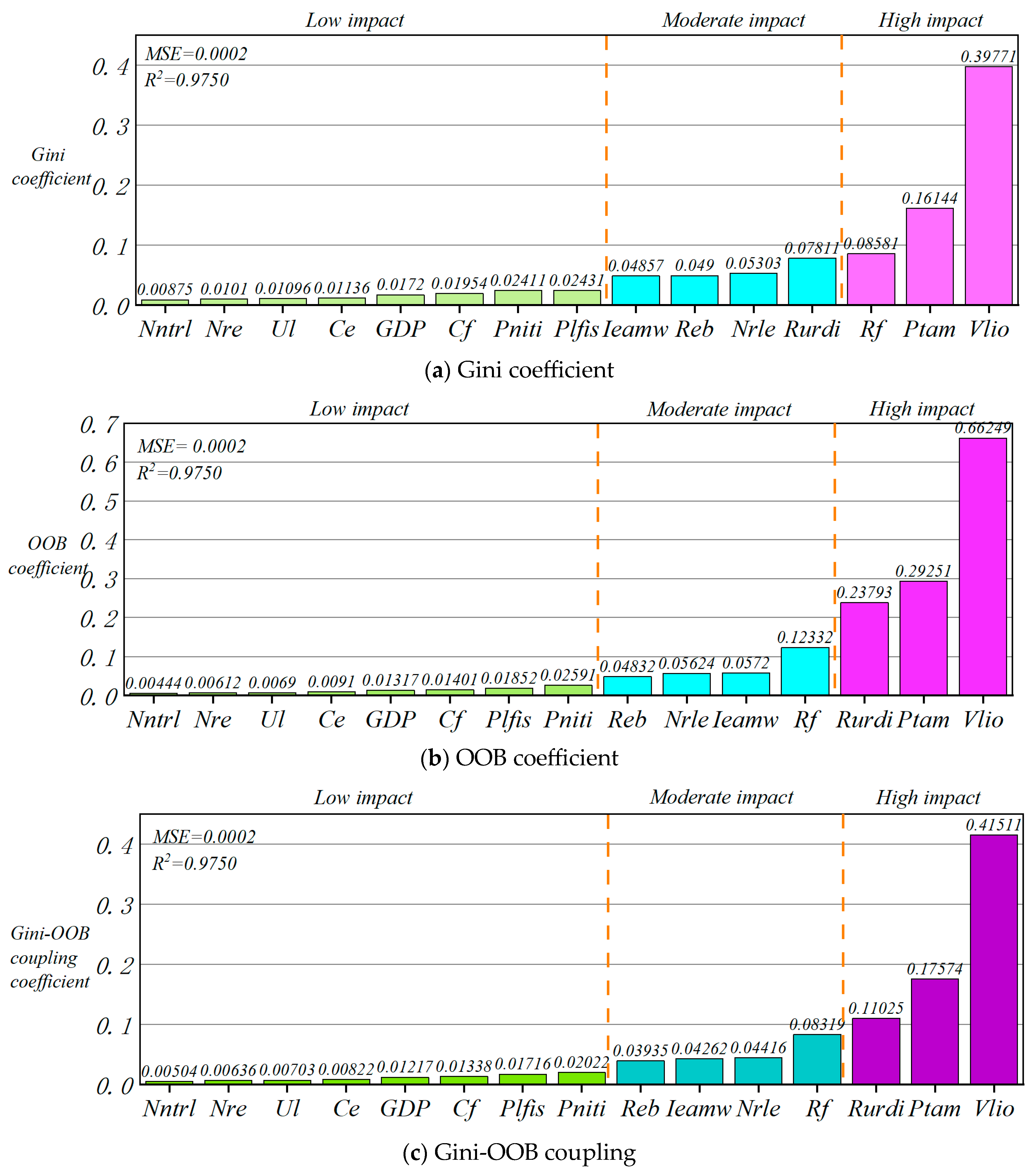
3.5.3. Gini-OOB Coefficient Coupling Calculation
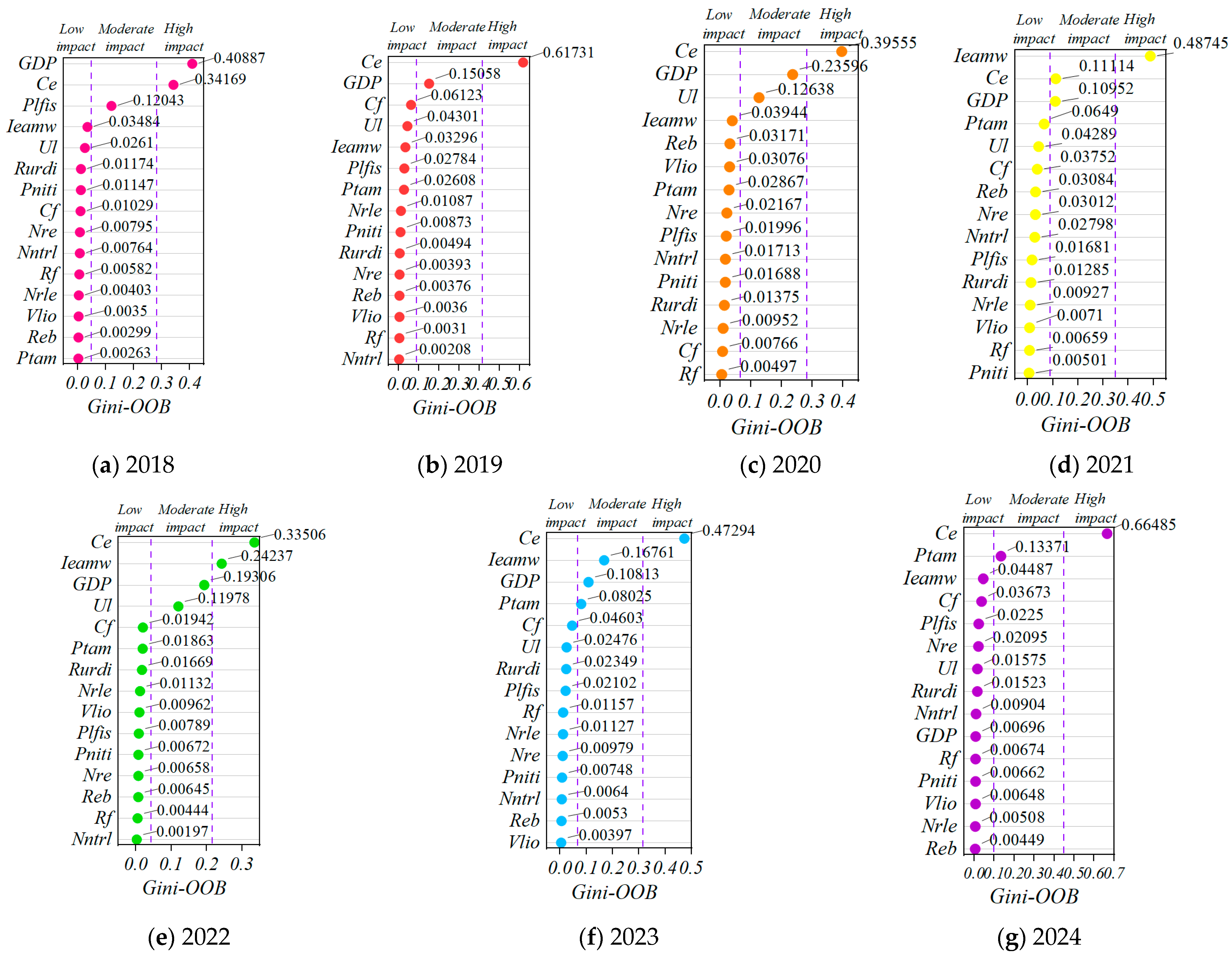
To further measure the degree of impact of rural labor economic indicators on digital inclusive finance, this paper uses the principle of minimum relative information entropy, removes unnecessary details, highlights key indicators, and constructs the Gini-OOB coupling coefficient [
81]. The combination of the two enables the selection of data features to no longer be dependent on a single criterion, making feature selection more objective and comprehensive. In addition to capturing feature correlations and lessening the subjectivity of Gini’s feature preferences, this also lessens unpredictability in the OOB error calculation process and enhances the degree of feature contribution value interpretation. This further optimizes model performance and lowers the risk of data overfitting.
The subjective weights
w1i, namely, the Gini coefficient, and objective weights
w2i, namely, the OOB coefficient, from the composite index were used to derive their combined weights
wi,
i = 1, 2, …,
m, namely, the Gini-OOB coupling coefficient. Among them,
wi should be as close as possible to
w1i and
w2i to reduce the overall information entropy. According to the principle of minimum relative information entropy, the Lagrange multiplier method is used to optimize the combination weight calculation equation. See the calculation formula in Equation (21):
3.6. Evaluation Metrics
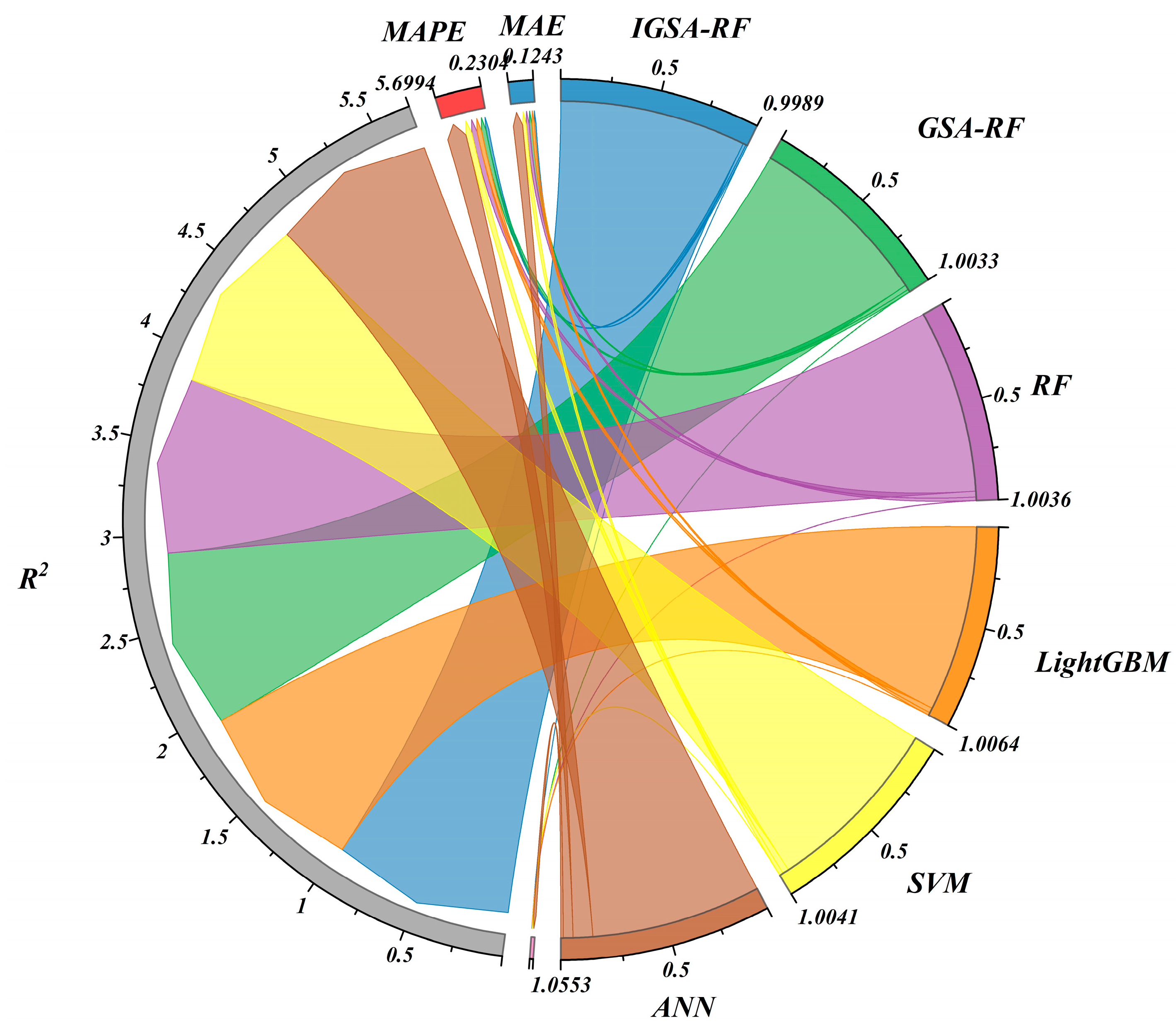
In the RF algorithm, two key parameters that influence model accuracy are the number of decision trees and the number of randomly selected features at each node, typically set to the square root of the total features. As the number of trees increases, the computational cost rises while improvements decrease. An accuracy test is used to select the optimal parameter. Irrelevant features can degrade the classification/regression performance, especially with noisy datasets, and can lead to overfitting. To address this, an accuracy test is essential for determining optimal feature subset sizes [
82]. To evaluate model performance, we use four metrics: Mean Squared Error (
MSE), Mean Absolute Error (
MAE), Mean Absolute Percentage Error (
MAPE), and
R2. The
MSE measures the average squared error, with lower values indicating higher accuracy. The
MAE provides the absolute error magnitude, while the
MAPE expresses error as a percentage.
R2 assesses the goodness of fit, with values closer to 1 indicating better model performance. These metrics ensure optimal feature selection and prevent overfitting. The formula is as follows:
where
yi is the target value,
is the predicted value, and
n is the number of datasets.


