Article

Efficient Numerical Methods for Reaction–Diffusion Problems Governed by Singularly Perturbed Fredholm Integro-Differential Equations

1
Amrita School of Physical Science, Amrita Vishwa Vidyapeetham, Coimbatore 641112, Tamil Nadu, India
2
Department of Mathematics and Statistics, College of Science, King Faisal University, Al Ahsa 31982, Saudi Arabia
*
Authors to whom correspondence should be addressed.
Mathematics 2025, 13(9), 1511; https://doi.org/10.3390/math13091511 (registering DOI)
Submission received: 10 April 2025 / Revised: 29 April 2025 / Accepted: 2 May 2025 / Published: 4 May 2025

Abstract

:
A set of singularly perturbed systems comprising Fredholm integro-differential equations associated with reaction–diffusion problems is considered. To approximate solutions to these systems, a second-order scheme for the derivatives and the trapezoidal rule for the integral terms are utilized. The discretization is performed on non-standard grids known as Shishkin-type meshes. The numerical method demonstrates a second-order rate of convergence with respect to small parameters in the equations, and error estimates are derived in the discrete maximum norm. Numerical experiments are conducted to verify the theoretical results.

1. Introduction

A differential equation with its primary term multiplied by a small parameter is a singularly perturbed differential equation (SPDE), and that parameter is a singular perturbation parameter. These equations form a very thin layer with the solution and its derivatives. These layers are called interior or boundary layers depending on the domain. The field of singular perturbation problems (SPPs) is highly significant due to their wide applicability in several science and technical aspects. The primary objective is to solve numerical methods for these problems to obtain accuracy and convergence.
Integro-differential equations (IDEs) are essential in several fields such as physics, engineering, biology and chemistry [1,2]. IDEs are classified according to their components: Fredholm integro-differential equations (FIDEs) are defined by integral terms that have a finite range, whereas Volterra integral-differential equations (VIDEs) consist of integral terms that are bounded by respected variables. A wide variety of analytical and numerical techniques have been developed to provide exact and approximate solutions for FIDEs. There are plenty of innovative numerical techniques specifically created for solving FIDEs that may be found in the literature. Chen et al. [3] proposed a Galerkin method for solving FIDEs and estimating the solution’s behavior using an analysis. Akyüz-Daşcioğlu et al. [4] solved linear FIDEs using the Taylor polynomial method.
In [5], fourth-order singularly perturbed convection–diffusion equations with integral boundary conditions were addressed using a non-uniform mesh approach. In [6], third-order singularly perturbed reaction–diffusion equations with integral boundary conditions are addressed using a Shishkin mesh. Singularly perturbed delay differential equations with integral boundary conditions are examined in [7]. Singularly perturbed delay differential equations of the convection–diffusion type with integral boundary conditions were solved using a finite difference scheme with a suitable piecewise Shishkin-type mesh in [8]. In [9], singularly perturbed parabolic partial differential equations with a spatial delay were constructed, and the right boundary plane was characterized by an integral boundary condition on a rectangular domain using a piecewise uniform mesh. Singularly perturbed systems of delay differential equations of the reaction–diffusion type with integral boundary conditions were addressed in [10]. Singularly perturbed mixed-delay differential equations are examined using a Shishkin mesh and a Bakhvalov–Shishkin mesh in [11]. Cimen et al. [12] devised a technique for computing singularly perturbed FIDE (SPFIDE) boundary value problems. Şevgin developed a numerical solution for a nonlinear SPVIDE with a boundary layer in [13]. Amiraliyev et al. [14] developed a method for calculating error estimates that were consistent across different parameters in estimating the solutions for an SPFIDE, with theoretical limits on the continuous solution and its derivative, and also developed a customized differentiation technique that was applied to a Shishkin mesh [15]. Durmaz et al. [16] tackled reaction–diffusion problems in SPFIDEs using a fitted homogeneous-type difference scheme on a Shishkin mesh. Afterwards, it attained a non-optimal rate of convergence of the second order. Sekar Elango and his colleagues [17] successfully solved the reaction–diffusion problem in SPFIDEs, applying a central difference scheme to the second-order derivative part and using the integral component through a composite trapezoidal rule. Govindarao et al. [18] handled the reaction–diffusion problem in SPFIDEs by using integral boundary conditions in their solution approach. Numerical Methods for Singular Perturbation discussed in [19,20]. Error estimations for the finite element method on Bakhvalov–Shishkin triangular mesh in [21]. In practical applications, finite difference methods are employed to derive several approximate solutions, such as the time-fractional Black–Scholes option pricing model, which is resolved using the compact finite difference approach in [22]. In [23], a finite difference approach is employed in the temporal direction, followed by a local discontinuous Galerkin method in the spatial domain to address the variable-order fractional diffusion problem. The paper in [24] examines a high-order numerical technique for the variable order subdiffusion problem utilizing the Caputo–-Hadamard derivative. In [25,26], the existence of positive solutions for a quasilinear Schrödinger equation was established. This study also addressed the resolution of nonlinear elliptic and parabolic equations within weighted and mixed-norm Sobolev spaces in [27]. Our objective is to present an effective numerical solution for the following problem as the motivation for this research.
The following set of singularly perturbed systems, comprising Fredholm integro-differential equations associated with reaction–diffusion problems, is considered.
L ε u ( t ) ε d 2 d t 2 0 0 d 2 d t 2 u ( t ) + A ( t ) u ( t ) λ 0 1 K ( t , s ) u ( s ) d s = f ( t ) , t D ¯ = [ 0 , 1 ] ,
u ( 0 ) = u 1 ( 0 ) u 2 ( 0 ) , u ( 1 ) = u 1 ( 1 ) u 2 ( 1 ) ,
where
u ( t ) = u 1 ( t ) u 2 ( t ) , A ( t ) = a 11 ( t ) a 12 ( t ) a 21 ( t ) a 22 ( t ) , f ( t ) = f 1 ( t ) f 2 ( t ) .
Here, the functions f i ( t ) , a i j ( t ) are sufficiently smooth for i , j = 1 , 2 and 0 < ε 1 .
Find u = ( u 1 , u 2 ) T , u 1 , u 2 X * = C 0 ( D ¯ ) C 2 ( D ) such that
L ε u ( t ) : = L 1 u ( t ) + L 2 u ( t ) = f ( t ) , t ( 0 , 1 ) = D ,
where L 1 u = ε d 2 d t 2 0 0 d 2 d t 2 u ( t ) + A ( t ) u ( t ) , L 2 u = λ 0 1 K ( t , s ) u ( s ) d s and γ > K ( t , s ) L 2 [ 0 , 1 ] . It is assumed that a i j ( t ) 0 , i = j , a i j ( t ) 0 , i j , a i 1 ( t ) + a i 2 ( t ) β > λ γ > 0 , i = 1 , 2 , where λ represents a positive constant. According to the assumption, the reaction–diffusion problem (1) contains boundary layers around x = 0 and x = 1 .
Sekar Elango and colleagues previously addressed problem (1) as detailed in [17], employing a fitted homogeneous-type difference scheme on a Shishkin mesh, which resulted in a second-order convergence rate. The objective of this article is to numerically tackle the same problem (1) utilizing a central difference scheme for the second-order derivative and a composite trapezoidal rule for the integral component on fitted meshes, specifically Shishkin-type meshes. In this way, we also achieve an optimal second-order rate of convergence, expressed as C N 2 , applicable to the system of SPFIDEs.
The structure of this article is organized as follows. An exploration of the analytical method applied to the problem is detailed in Section 2. The development of non-uniform grid structures and their computational analysis are discussed in Section 3. Additionally, Section 4 provides tables and figures showcasing the numerical results, while the final observations and remarks of this study are found in Section 5. Within the context of this paper, we denote C to signify a collection of positive constants, with ε being constants that do not depend on any other variables. We employ the standard supremum norm for our analysis, denoted by | . | , which is mathematically expressed as f D = sup ( y ) D | f ( y ) | .

2. Analytical Results

Theorem 1
(Maximum principle). Given ψ ( t ) = ( ψ 1 ( t ) , ψ 2 ( t ) ) T as any function in X = C 0 ( D ¯ ) C 2 ( D ) such that ψ j ( 0 ) 0 , j = 1 , 2 , ψ j ( 1 ) 0 , j = 1 , 2 , L ε ψ ( t ) 0 , t D , then it follows that ψ j ( t ) 0 , t D ¯ , j = 1 , 2 .
Proof. 
Ref [17]. □
Note: Uniqueness is ensured by the maximum principle.
Corollary 1
(Stability result). Let w = ( w 1 , w 2 ) T , w 1 , w 2 X * we have,
(i) 
w i ( t ) C max max j = 1 , 2 { w j ( 0 ) } , max j = 1 , 2 { w j ( 1 ) } , max { sup t D L ε u ( t ) } .
(ii) 
| u i ( k ) ( t ) | C ε k / 2 , i = 1 , 2 , k { 1 , 2 , 3 }
Proof. 
The present corollary can be proven using the method from the proof outlined in Corollary 1 of the referenced paper [17]. □
The lemma presents the inequality of the bound of derivatives of the solution u ( t ) .
Lemma 1.
If y ( t ) and z ( t ) are the solutions of the smooth and singular components u ( t ) , then the following estimations apply.
(i) 
y ( k ) ( t ) C ( 1 + ε ( k 2 ) / 2 ) .
(ii) 
z L ( k ) ( t ) C ε k / 2 e t β / ε .
(iii) 
z R ( k ) ( t ) C ε k / 2 e ( 1 t ) β / ε , w h e r e k = 1 , 2 , 3 , 4 .
Proof. 
(i) The proof is available in [17].
(ii) Consider ψ ± ( t ) = C e t β / ε ± z L ( t ) . Note that ψ ± ( 0 ) 0 and ψ ± ( 1 ) 0 . We have
L ψ ± ( t ) = C e t β / ε ε ( β / ε ) + A ( t ) λ 0 1 C K ( t , s ) e s β / ε d s ± L z L ( t ) 0
Theorem 1 establishes that ψ ± ( t ) 0 ; hence,
z L ( t ) C e t β / ε .
The proof for the derivative limits of the left singular component uses the same logic as that stated in [17], yielding
z L ( k ) ( t ) C e t β / ε ε k / 2 .
(iii) Similarly to the previous case, it can be proven that
| z R ( k ) ( t ) | C ε k / 2 e ( 1 t ) β / ε .

3. Discretization Grid Points

In this study, we employ the central difference scheme to approximate the second-order derivatives and the trapezoidal rule for the integral terms. These methods are chosen based on their established accuracy and suitability for solving SPFIDEs.
The central difference scheme is widely recognized for its second-order accuracy in approximating second-order derivatives. It is particularly effective when applied to uniformly spaced grids. In the case of singularly perturbed equations, however, the central difference scheme can struggle near boundary layers due to the rapid changes in the solution. To mitigate this, we employ Shishkin-type meshes, which refine the grid near the boundary layers where the solution exhibits steep gradients. This mesh adaptation ensures that the central difference scheme maintains its accuracy even in regions with rapid variations, leading to an optimal performance across the entire domain.
The central difference method’s use on the Shishkin mesh guarantees that the solution is accurately captured even in the boundary layer regions, where singular perturbations typically cause rapid changes. This combination of the central difference scheme and the adaptive mesh refinement results in a second-order convergence rate for the solution, which is consistent with the theoretical expectations.
The trapezoidal rule is applied to approximating the integral terms in the Fredholm integro-differential equations. This method is chosen because it provides second-order accuracy for numerical integration, making it a reliable choice for discretizing the integral components of the equation. The trapezoidal rule is particularly effective for finite-range integrals, such as those encountered in Fredholm equations, where the integral terms involve a bounded domain.
Additionally, the trapezoidal rule works well in combination with the Shishkin-type mesh, where grid refinement enhances the accuracy of the integration near regions with boundary layers. This synergy between the trapezoidal rule and the Shishkin mesh ensures that the integral components are computed with high accuracy, even in areas where the solution experiences rapid changes.
The use of both the central difference scheme for second-order derivatives and the trapezoidal rule for the integral components ensures a well-balanced and efficient approach to solving the singularly perturbed system. These methods are second-order accurate and provide a uniformly convergent numerical scheme. By jointly addressing the differential and integral components of the equations, they enhance the precision of the solutions while optimizing the computational efficiency.
This combined approach allows us to achieve uniform convergence with a second-order precision across the entire domain, while ensuring the solution’s validity even in the presence of boundary layers induced by the singular perturbation parameter.

3.1. The Shishkin Mesh (S-Mesh)

Let σ = min 1 4 , σ 0 ε β ln ( N ) describe the transition parameter. Assume ε N 1 and σ 0 > 0 as the user’s chosen constant. The detailed S-mesh is given in [19,20]. The mesh points should be specified as D ¯ N = { t 0 , t 1 , t 2 , t n } [ 0 , 1 ] .
t i = i H 1 , for i = 0 , , N 4 , σ + i N 1 4 H 2 , for i = N 4 + 1 , , 3 N 4 , 1 ( N i ) H 1 , for i = 3 N 4 + 1 , , N ,
Here, H 1 = 4 σ N and H 2 = 2 ( 1 2 σ ) . The step size in space is determined by h i = t i t i 1 .

3.2. The Bakhvalov–Shishkin Mesh (BS-Mesh)

In [21], extensive information on the construction of a BS-mesh is provided. The mesh is
t i = σ 0 ε β ln ϑ ( i N ) + 1 , for i = 0 , , N / 4 , σ 1 + 4 i N 1 1 / 2 σ 1 , for i = N 4 + 1 , , 3 N 4 , 1 + σ 0 ε β ln ϑ ( 1 i N ) + 1 , for i = 3 N 4 + 1 , , N ,
where σ 1 = min 1 4 , σ 0 ε β ln min { ε 1 , N } and ϑ = 4 exp β σ 1 / ( σ 0 ε ) 1 . We take the step size as h i = t i t i 1 .

3.3. Numerical Experiments: Methods and Analysis

In the context of a given mesh function ϕ i , which is defined by ϕ i = ϕ ( t i ) , the forward, backward and central difference operators are specified as
D t + ϕ i = ϕ i + 1 ϕ i h i + 1 , D t ϕ i = ϕ i ϕ i 1 h i , D t 0 ϕ i = ϕ i + 1 ϕ i 1 h i + 1 + h i ,
The approximate second-order derivative operator, combining the forward and backward differences, is defined as
D t + D t ϕ i = 2 h i + h i + 1 ϕ i + 1 ϕ i h i + 1 ϕ i ϕ i 1 h i .
To discretize problem (1), we apply the central difference scheme for the second-order derivative and the trapezoidal rule for the integral component across the domain D N = { t 1 , t 2 , , t N 1 } .
The numerical scheme that has been proposed is presented in the form of a discretized equation, which typically would involve the application of the difference operators and the integral approximation method described earlier. The scheme will incorporate these into an equation that discretizes the original problem (1) over the domain D N . The exact form of the numerical scheme would be provided in the paper or article where it were being proposed.
L ε N U i ε D t + D t 0 0 D t + D t U ( t i ) + A ( t i ) U ( t i ) λ j = 0 N τ j K i , j U ( s j ) = f ( t i ) ,
U ( t 0 ) = U 1 ( 0 ) U 2 ( 0 ) , U ( t N ) = U 1 ( 1 ) U 2 ( 1 ) , t i D ¯ N = [ 0 , 1 ] ,
where
U ( t i ) = U i = U 1 ( t i ) U 2 ( t i ) , A ( t i ) = a 11 ( t i ) a 12 ( t i ) a 21 ( t i ) a 22 ( t i ) , f ( t i ) = f 1 ( t i ) f 2 ( t i ) .
where
τ 0 = h 0 2 , τ j = h j + h j + 1 2 , j = 1 , 2 , , N 1 , τ N = h N 2 .
Theorem 2.
Let t i D N be a mesh point. If Φ ( t i ) = ( Φ 1 ( t i ) , Φ 2 ( t i ) ) T satisfies and Φ ( t 0 ) 0 , Φ ( t N ) 0 , L ε N Φ ( t i ) 0 , tShen Φ ( t i ) 0 , t i D ¯ N .
Proof. 
Define the step function S ( t i ) = ( S 1 ( t i ) , S 2 ( t i ) ) T , as S 1 ( t i ) = 1 + t i = S 2 ( t i ) Note that S ( t i ) > 0 , t i D ¯ N , S ( t i ) > 0 , L N S ( t i ) > 0 , t i D N . Let
μ = max max t i D ¯ N Φ 1 ( t i ) S 1 ( t i ) , max t i D ¯ N Φ 2 ( t i ) S 2 ( t i ) .
Then, one t k D ¯ N exists such that Φ 1 ( t k ) + μ S 1 ( t k ) = 0 or Φ 2 ( t k ) + μ S 2 ( t k ) = 0 or both. We have Φ j ( t i ) + μ S j ( t i ) 0 , t i D ¯ N , j = 1 , 2 . Therefore, either ( Φ 1 + μ S 1 ) or ( Φ 2 + μ S 2 ) attains a minimum at t i = t k . In case of contradiction, take μ > 0 .
Case (i): t k = t 0 and t k = t N
0 < ( Φ j + μ S j ) ( t 0 ) = 0 = Φ j ( t k ) + μ S ( t k ) = 0
Case (ii): t k D N
0 < L ε N ( Φ j + μ S j ) ( t k ) = ε D t + D t 0 0 D t + D t ( Φ j + μ S j ) ( t k ) + A ( t i ) ( Φ j + μ S j ) ( t k ) λ h 1 K i , 1 ( Φ j + μ S j ) ( t 1 ) + + h N K i , N ( Φ j + μ S j ) ( t N ) 0 .
It contradicts itself. □
Corollary 2.
Let U ( t i ) = ( U 1 ( t i ) , U 2 ( t i ) ) T be any mesh function. Then,
U k ( t i ) C max max j = 1 , 2 { U j ( 0 ) } , max j = 1 , 2 { U j ( 1 ) } , max { sup t i D L ε N U ( t i ) } , t i D ¯ N , k = 1 , 2 .
Proof. 
This assertion can be straightforwardly demonstrated by applying the results of Theorem 2. □

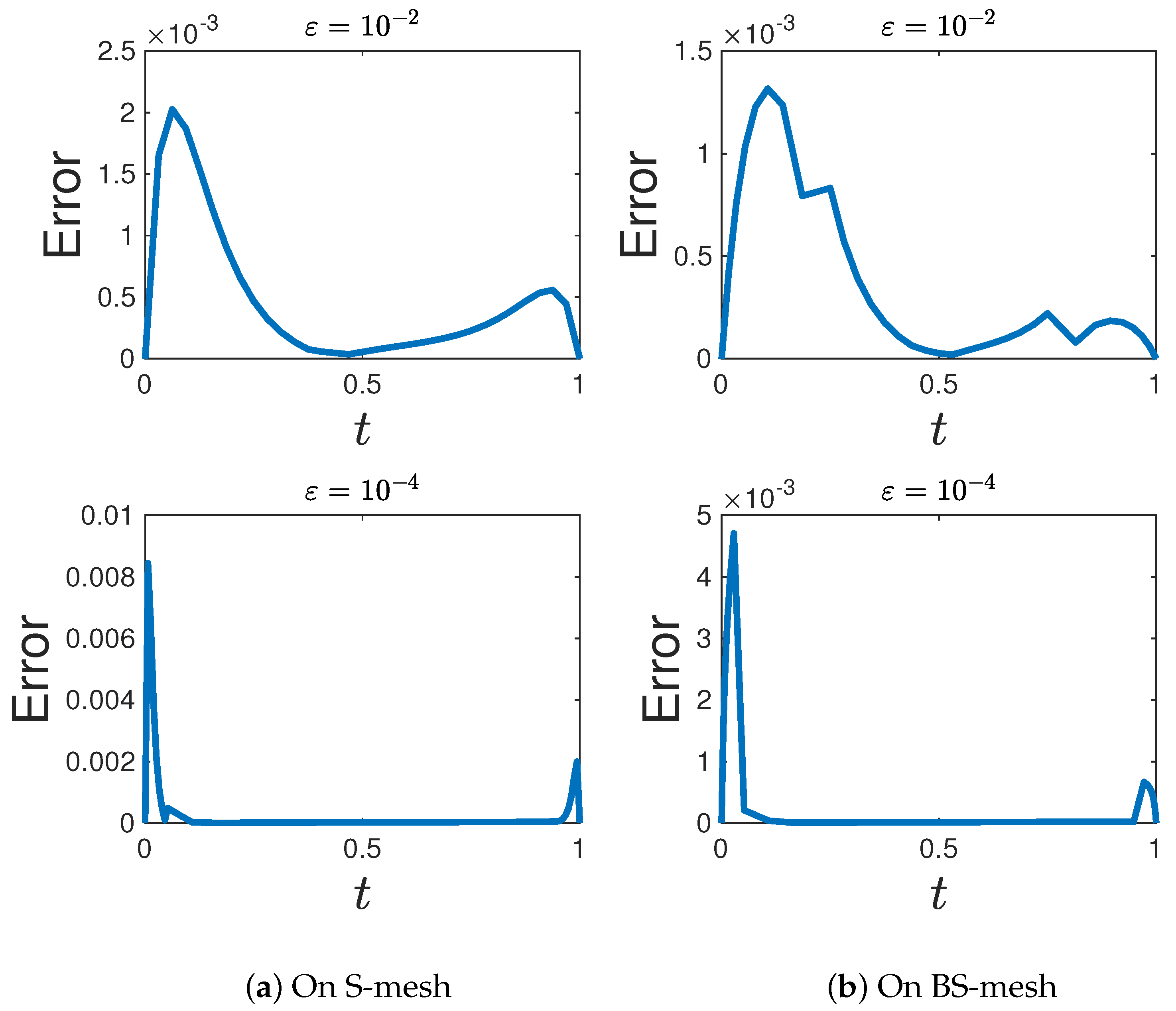
3.4. Error Estimation Techniques for Difference Schemes in Numerical Methods

Theorem 3.
Let u and U be the solutions to (1) and (2), respectively; then, the following estimate is satisfied by the numerical scheme’s error (2)
max i | ( u U ) ( t i ) | C ( N 1 ln N ) 2 o n   S - m e s h , C N 2 o n   B S - m e s h
for i = 1 , , N 1 .
Proof. 
The discrete solution U is composed of two parts: the smooth component V and the singular component W . The error associated with this solution can be expressed as follows:
L N ( U u ) = L 1 N ( U u ) + L 2 N ( U u ) .
According to Miller [19],
L 1 N ( U u ) C ( N 1 ln N ) 2 .
Now, for the operator L 2 , the following holds:
L 2 N ( U u ) = L 2 N ( V v ) + L 2 N ( W w ) .
An error analysis on smooth components:
L 2 N ( V i v i ) = λ j = 0 N τ j K i j V j λ 0 1 K ( t , s ) v ( s ) d s , = λ j = 0 N τ j K i j v j λ 0 1 K ( t i , s ) v ( s ) d s , C j = 1 N t j 1 t j ( t j ξ ) ( ξ t j 1 ) ( 1 + | v ( ξ ) | + | v ( ξ ) | ) d ξ , C N 1 ( h ) , L 2 N ( V i v i ) C N 2 .
By leveraging the stability result, it follows that
| V ( t i ) v ( t i ) | C N 2 ln N .
An error analysis on layer components:
L 2 N ( W i w i ) = L 2 N ( W ( t i ) ) L 2 N ( w ( t i ) ) , = λ j = 0 N τ j K i j W j λ 0 1 K ( t i , s ) w ( s ) d s , = λ j = 0 N τ j K i j W j λ 0 1 K ( t i , s ) w ( s ) d s , C j = 1 N t j 1 t j ( t j ξ ) ( ξ t j 1 ) ( 1 + | w ( ξ ) | + | w ( ξ ) | ) d ξ , C j = 1 N t j 1 t j ( t j ξ ) ( ξ t j 1 ) ( 1 ε ) ( e t β / ε + e ( 1 t ) β / ε ) d ξ , C N 1 h 3 ε , L 2 N ( W i w i ) C N 2 ln 2 N .
According to the stability results,
| W ( t i ) w ( t i ) | C N 2 ln 2 N .
Therefore,
| U ( t i ) u ( t i ) | = | V ( t i ) v ( t i ) | + | W ( t i ) w ( t i ) | C N 2 ln 2 N .
Similarly, on the BS-mesh, we obtain
| U ( t i ) u ( t i ) | = | V ( t i ) v ( t i ) | + | W ( t i ) w ( t i ) | C N 2 .

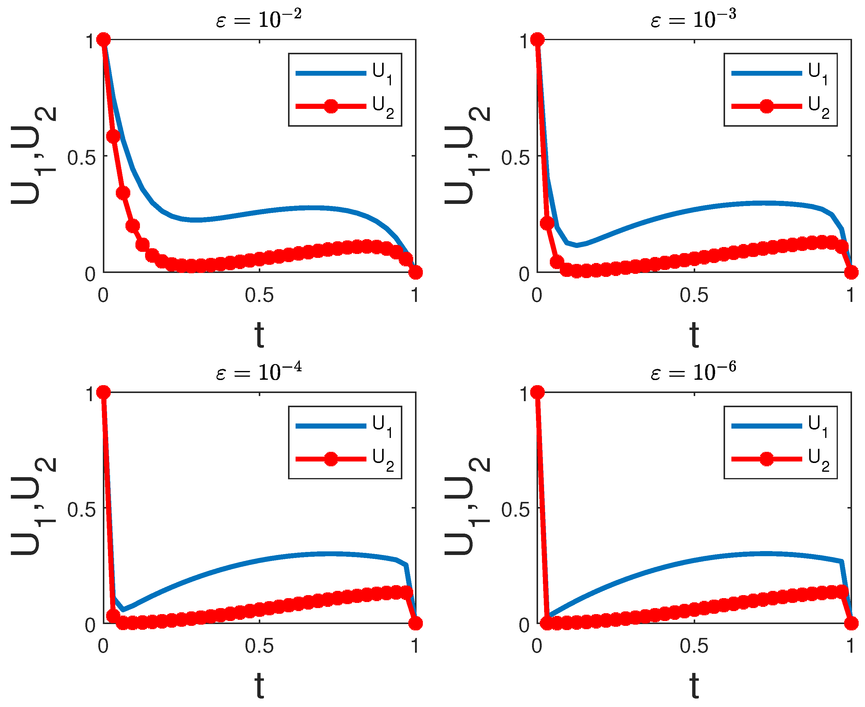
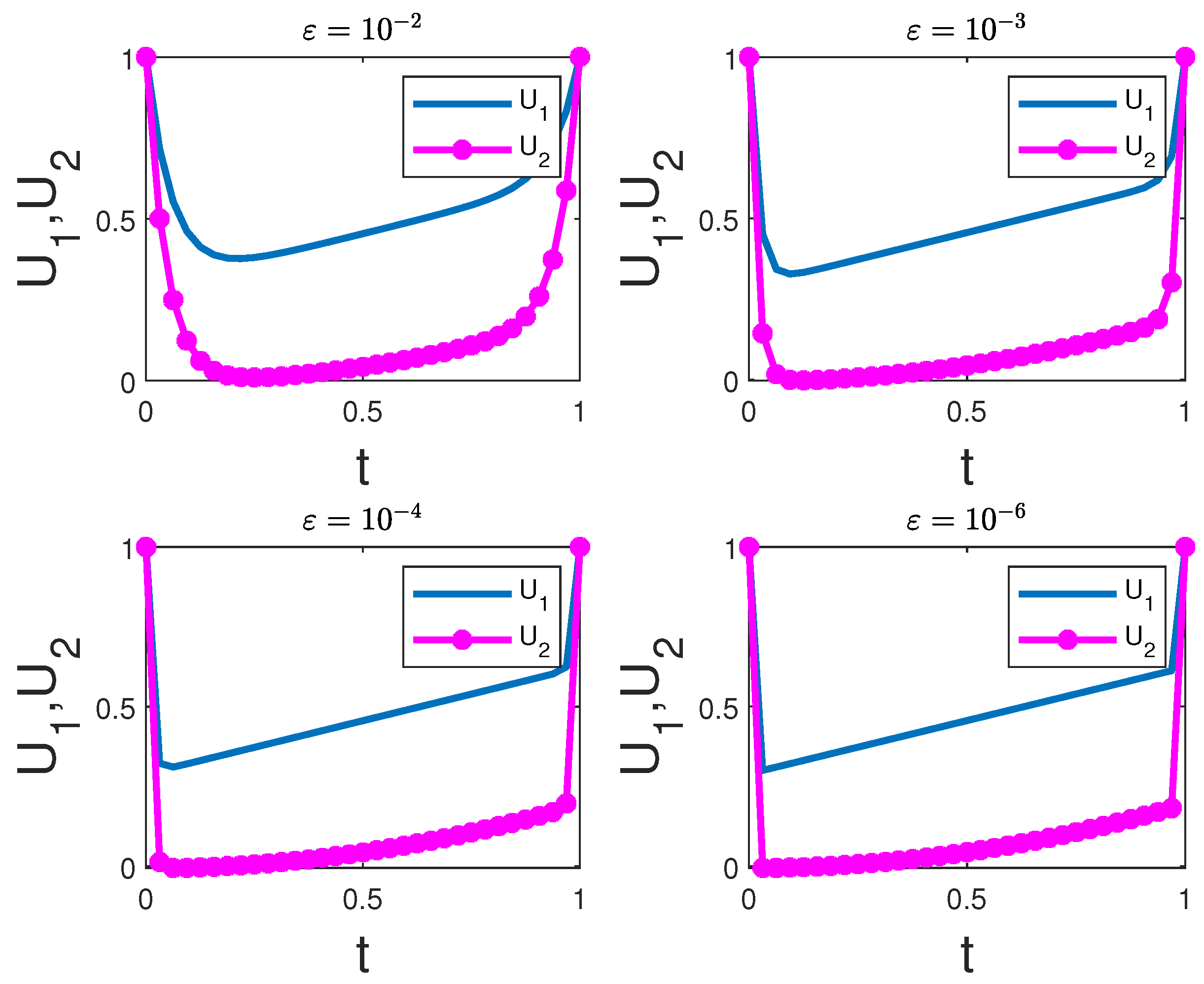
4. Computational Simulations

The proposed method, as described in Equation (2), was employed to solve a test problem, with the findings and outcomes discussed in this section of the paper. We used MATLAB 2024 with 16 GB of RAM to obtain the computational results.
Example 1.
Consider the SPFIDEs below:
ε u 1 ( t ) + ( 2 e t ) u 1 ( t ) 0.5 0 1 t u 1 ( s ) d s = t cos ( t ) , t ( 0 , 1 ) , ε u 2 ( t ) + ( 4 e t ) u 2 ( t ) 0.5 0 1 t u 2 ( s ) d s = t 2 cos ( t ) , t ( 0 , 1 ) , u 1 ( 0 ) = 1 , u 1 ( 1 ) = 0 , u 2 ( 0 ) = 1 , u 2 ( 1 ) = 0 .
Example 2.
Consider the SPFIDEs below:
ε u 1 ( t ) + 3 u 1 ( t ) 0.5 0 1 s u 1 ( s ) d s = x + 1 , t ( 0 , 1 ) , ε u 2 ( t ) + 5 u 2 ( t ) 0.5 0 1 s u 2 ( s ) d s = x 2 , t ( 0 , 1 ) , u 1 ( 0 ) = 1 , u 1 ( 1 ) = 1 , u 2 ( 0 ) = 1 , u 2 ( 1 ) = 1 .
Given that the exact solutions are not available for Examples 1 and 2, we employ the double-mesh principle to estimate the pointwise errors and verify the ε -uniform convergence. This principle operates as follows.
Let U ˜ ( t i ) denote the numerical solutions obtained on a Shishkin-type mesh that utilizes a fixed transition parameter. The mesh in question is constructed based on the D ¯ 2 N grid.
To ascertain the maximum pointwise error for each value of ε , both before and after extrapolation, we use the following expression: E ε N = max ( t i ) D ¯ N U ( t i ) U ˜ ( t i ) . The rate of convergence is then determined by the formula P ε N = log 2 E ε N E ε 2 N , which defines the order of convergence by comparing the maximum error on the original mesh with that on a mesh with double the number of intervals.
The numerical solutions for Examples 1 and 2 across various values of ε are depicted in Figure 1 and Figure 2, respectively. These illustrations reveal that as ε diminishes, boundary layers emerge near t = 0 and at t = 1 . The magnitude of the error for Example 1 is represented in Figure 3 on both the S-mesh and the BS-mesh. The error on the BS-mesh is notably smaller in comparison to that on the S-mesh, as can be seen in the figure. Figure 4 illustrates the peak pointwise errors on both the S-mesh and BS-mesh using a log-log scale to visually demonstrate the numerical progression of the convergence of Example 1.
Table 1 and Table 2 present the estimated maximum pointwise errors and the rate of convergence for Examples 1 and 2 when employing the proposed numerical method. The data from the table indicate that the convergence rate is approximately two (considering the logarithmic factor) on the S-mesh, whereas on the BS-mesh, the rate of convergence achieves a consistent value of two. It is also evident from the table that the precision of the solution is superior on the BS-mesh in contrast to that on the S-mesh.

5. Conclusions

This paper addresses the numerical solution for a singularly perturbed system of Fredholm integro-differential equations. For the derivative part, a central difference scheme is applied, while the integral component is handled using the trapezoidal rule on non-uniform meshes, such as the Shishkin mesh and the Bakhvalov–Shishkin mesh. It is demonstrated that the numerical scheme achieves uniform convergence in relation to the small parameter ε , and it delivers second-order precision. To validate the effectiveness of this method, the numerical scheme is applied to a specific example.
Future work could focus on extending the proposed numerical method to handling nonlinear singularly perturbed Fredholm integro-differential equations, as these introduce additional complexities. Moreover, adaptive mesh refinement strategies could be explored to improve the accuracy near the boundary layers, and higher-order numerical schemes could be investigated to enhance the convergence rate. Another avenue for improvement is the application of parallel computing techniques to addressing the computational challenges posed by large-scale systems. Additionally, comparing the performance of the proposed method with other numerical techniques, such as finite element or spectral methods, would provide valuable insights into its relative strengths and weaknesses. These directions offer potential to advance the current methodology and broaden its applicability to more complex systems.

Author Contributions

Formal analysis, H.Z.; Writing—original draft, S.E.; Writing—review & editing, M.A.; Visualization, L.G. All authors have read and agreed to the published version of the manuscript.

Funding

This work was supported by the Deanship of Scientific Research, Vice Presidency for Graduate Studies and Scientific Research, King Faisal University, Saudi Arabia [Grant No. KFU251712].

Data Availability Statement

The original contributions presented in this study are included in the article. Further inquiries can be directed to the corresponding author.

Conflicts of Interest

The authors declare that they have no competing interests concerning the publication of the manuscript.

References

  1. Rahman, M. Integral Equations and Their Applications; WIT Press: Southampton, UK, 2007. [Google Scholar]
  2. Wazwaz, A.M. Linear and Nonlinear Integral Equations; Springer: Berlin/Heidelberg, Germany, 2011. [Google Scholar]
  3. Chen, J.; Huang, Y.; Rong, H.; Wu, T.; Zeng, T. A multiscale Galerkin method for second-order boundary value problems of Fredholm integro-differential equation. J. Comput. Appl. Math. 2015, 290, 633–640. [Google Scholar] [CrossRef]
  4. Akyüz-Daşcioğlu, A.; Sezer, M. A Taylor polynomial approach for solving the most general linear Fredholm integrao-differential-difference equations. Math. Methods Appl. Sci. 2012, 35, 839–844. [Google Scholar] [CrossRef]
  5. Raja, V.; Sekar, E.; Priya, S.S.; Unyong, B. Fitted mesh method for singularly perturbed fourth order differential equation of convection diffusion type with integral boundary condition. AIMS Math. 2023, 8, 16691–16707. [Google Scholar] [CrossRef]
  6. Raja, V.; Tamilselvan, A.; Jayalakshmi, G.J.; Sekar, E. Fitted finite difference technique for singularly perturbed reaction diffusion equations of third order with integral boundary condition. Int. J. Numer. Methods Fluids. 2023, 95, 1487–1501. [Google Scholar] [CrossRef]
  7. Sekar, E. Second order singularly perturbed delay differential equations with non-local boundary condition. J. Comput. Appl. Math. 2023, 417, 114498. [Google Scholar]
  8. Sekar, E.; Tamilselvan, A. Singularly perturbed delay differential equations of convection–diffusion type with integral boundary condition. J. Appl. Math. Comput. 2019, 59, 701–722. [Google Scholar] [CrossRef]
  9. Sekar, E.; Tamilselvan, A.; Vadivel, R.; Gunasekaran, N.; Zhu, H.; Cao, J.; Li, X. Finite difference scheme for singularly perturbed reaction diffusion problem of partial delay differential equation with non local boundary condition. Adv. Differ. Equ. 2021, 2021, 151. [Google Scholar]
  10. Sekar, E.; Tamilselvan, A. Parameter uniform method for a singularly perturbed system of delay differential equations of reaction–diffusion type with integral boundary conditions. Int. J. Appl. Math. 2019, 5, 85. [Google Scholar] [CrossRef]
  11. Sekar, E.; Unyong, B. Numerical Scheme for Singularly Perturbed Mixed Delay Differential Equation on Shishkin Type Meshes. Fractal. Fract. 2023, 7, 43. [Google Scholar]
  12. Cimen, E.; Cakir, M. A uniform numerical method for solving singularly perturbed Fredholm integro-differential problem. Comput. Appl. Math. 2021, 40, 42. [Google Scholar] [CrossRef]
  13. Şevgin, S. Numerical solution of a singularly perturbed Volterra integro-differential equation. Adv. Differ. Equ. 2014, 2014, 171. [Google Scholar] [CrossRef]
  14. Amiraliyev, G.M.; Durmaz, M.E.; Kudu, M. Uniform convergence results in singularly perturbed Fredholm integro-differential equations. J. Math. Anal. 2018, 9, 55–64. [Google Scholar]
  15. Amiraliyev, G.M.; Durmaz, M.E.; Kudu, M. Fitted second order numerical method for a singularly perturbed Fredholm integro-differential equation. Bull. Belgian Math. Soc. Simon Stevin 2020, 27, 71–88. [Google Scholar] [CrossRef]
  16. Durmaz, M.E.; Amiraliyev, G.M. A robust numerical method for a singularly perturbed Fredholm integro-differential equation. Mediterr. J. Math. 2021, 18, 24. [Google Scholar] [CrossRef]
  17. Sekar, E.; Govindarao, L.; Mohapatra, J.; Vadivel, R.; Hu, N. Numerical analysis for second order differential equation of reaction-diffusion problems in viscoelasticity. Alex. Eng. J. 2024, 92, 92–101. [Google Scholar]
  18. Govindarao, L.; Ramos, H.; Elango, S. Numerical scheme for singularly perturbed Fredholm integro-differential equations with non-local boundary conditions. Comp. Appl. Math. 2024, 43, 126. [Google Scholar] [CrossRef]
  19. Miller, J.J.H.; O’Riordan, E.; Shishkin, I.G. Fitted Numerical Methods for Singular Perturbation Problems; World Scientific: Singapore, 2012. [Google Scholar]
  20. Shishkin, G.I.; Shishkina, L.P. Difference Methods for Singular Perturbation Problems; CRC Press: Boca Raton, FL, USA, 2009. [Google Scholar]
  21. Liu, X.; Yang, M. Error estimations in the balanced norm of finite element method on Bakhvalov–Shishkin triangular mesh for reaction–diffusion problems. Appl. Math. Lett. 2022, 123, 107523. [Google Scholar] [CrossRef]
  22. Feng, Y.; Zhang, X.; Chen, Y.; Wei, L. A compact finite difference scheme for solving fractional Black-Scholes option pricing model. J. Inequalities Appl. 2025, 2025, 35. [Google Scholar] [CrossRef]
  23. Wei, L.; Yang, Y. Optimal order finite difference/local discontinuous Galerkin method for variable-order time-fractional diffusion equation. J. Comput. Appl. Math. 2021, 383, 113129. [Google Scholar] [CrossRef]
  24. Li, W.; Wei, L. Analysis of Local Discontinuous Galerkin Method for the Variable-order Subdiffusion Equation with the Caputo–Hadamard Derivative. Taiwan J. Math. 2024, 28, 1095–1110. [Google Scholar] [CrossRef]
  25. Chu, C.; Liu, H. Existence of positive solutions for a quasilinear Schrödinger equation. Nonlinear Anal. Real World Appl. 2018, 44, 118–127. [Google Scholar] [CrossRef]
  26. Liu, H.; Zhao, L. Existence results for quasilinear Schrödinger equations with a general nonlinearity. Commun. Pure Appl. Anal. 2020, 19, 3429–3444. [Google Scholar] [CrossRef]
  27. Dong, H.; Krylov, N.V. Fully nonlinear elliptic and parabolic equations in weighted and mixed-norm Sobolev spaces. Calc. Var. 2019, 58, 145. [Google Scholar] [CrossRef]
Figure 1. Plots of the solutions for ε = { 10 2 , 10 3 , 10 4 , 10 6 } with N = 64 using the S-mesh of Example 1.
Mathematics 13 01511 g001
Figure 2. Plots of the solutions for ε = { 10 2 , 10 3 , 10 4 , 10 6 } with N = 64 using the S-mesh of Example 2.
Mathematics 13 01511 g002
Figure 3. Error plots for ε = { 10 2 , 10 4 } with N = 64 using the S-mesh and BS-mesh of Example 1.
Mathematics 13 01511 g003
Figure 4. Log-log plots of ε = { 10 2 , 10 3 , 10 6 } and S-mesh and BS-mesh for Example 1.
Mathematics 13 01511 g004
Table 1. E ε N and P ε N using the proposed approach for Example 1.
Number of Intervals N
ε 3264128256512
S-mesh 1 e 1 2.8991e-47.2784e-51.8207e-54.5536e-61.1385e-6
1.99391.99911.99941.99992.0032
1 e 2 3.1597e-38.0857e-42.0377e-45.1082e-51.2775e-5
1.96641.98851.99601.99951.9997
1 e 3 1.2628e-24.7229e-31.7147e-35.1814e-41.3024e-4
1.41891.46171.72661.99221.9978
1 e 4 1.2692e-24.7495e-31.7244e-35.7464e-41.8352e-4
1.41801.46171.58531.64671.6942
1 e 5 1.2711e-24.7574e-31.7273e-35.7560e-41.8383e-4
1.41781.46171.58531.64671.6942
1 e 6 1.2717e-24.7574e-31.7273e-35.7560e-41.8383e-4
1.41771.46171.58531.64671.6942
1 e 7 1.2711e-24.7574e-31.7273e-35.7560e-41.8383e-4
1.41781.46171.58531.64671.6942
1 e 8 1.2711e-24.7574e-31.7273e-35.7560e-41.8383e-4
1.41781.46171.58531.64671.6942
BS-mesh 1 e 1 2.5218e-46.3134e-51.5789e-53.9477e-69.8694e-7
1.99801.99951.99992.00001.9994
1 e 2 5.9839e-41.5376e-43.8722e-59.6987e-62.4258e-6
1.96041.98941.99731.99931.9998
1 e 3 1.8841e-34.6083e-41.1441e-42.8558e-57.1366e-6
2.03162.01002.00222.00062.0001
1 e 4 1.9838e-34.9614e-41.2470e-43.1313e-57.7980e-6
1.99951.99221.99372.00561.6393
1 e 5 2.0044e-34.9941e-41.2557e-43.1564e-57.9166e-6
2.00491.99171.99221.99531.9978
1 e 6 2.0117e-35.0056e-41.2586e-43.1629e-57.9342e-6
2.00681.99171.99251.99511.9974
1 e 7 2.0140e-35.0095e-41.2595e-43.1651e-57.9399e-6
2.00741.99181.99261.99501.9974
1 e 8 2.0140e-35.0095e-41.2595e-43.1651e-57.9399e-6
2.00741.99181.99261.99501.9974
Table 2. E ε N and P ε N using the proposed approach for Example 2.
Number of Intervals N
ε 3264128256512
S-mesh 1 e 1 5.4048e-41.3640e-43.4136e-58.5361e-62.1344e-6
1.98641.99851.99961.99981.9976
1 e 2 4.9656e-31.3671e-33.4531e-48.6660e-52.1686e-5
1.86081.98521.99451.99861.9996
1 e 3 1.1577e-24.3537e-31.5639e-35.1834e-41.6483e-4
1.41101.47711.59321.65291.6933
1 e 4 1.1613e-24.3696e-31.5690e-35.2000e-41.6532e-4
1.41021.47761.59331.65321.6931
1 e 5 1.1624e-24.3744e-31.5706e-35.2050e-41.6547e-4
1.40991.47781.59331.65331.6931
1 e 6 1.1627e-24.3759e-31.5711e-35.2066e-41.6552e-4
1.40981.47781.59331.65331.6930
1 e 7 1.1628e-24.3764e-31.5712e-35.2071e-41.6553e-4
1.40981.47791.59331.65331.6930
1 e 8 1.1628e-24.3765e-31.5713e-35.2072e-41.6554e-4
1.40981.47791.59331.65331.6930
BS-mesh 1 e 1 4.1438e-41.0381e-42.5965e-56.4921e-61.6229e-6
1.99701.99931.99982.00011.9929
1 e 2 7.6187e-41.9758e-44.9562e-51.2401e-53.1008e-6
1.94711.99521.99881.99971.9999
1 e 3 1.7239e-34.4728e-41.1361e-42.8444e-57.1159e-6
1.94641.97711.99781.99901.9998
1 e 4 1.7702e-34.7562e-41.2232e-43.0724e-57.5141e-6
1.89601.95921.99322.03172.1596
1 e 5 1.7760e-34.7700e-41.2289e-43.1053e-57.7940e-6
1.89651.95661.98451.99432.0014
1 e 6 1.7775e-34.7731e-41.2297e-43.1077e-57.8059e-6
1.89691.95661.98441.99321.9969
1 e 7 1.7780e-34.7741e-41.2300e-43.1082e-57.8071e-6
1.89701.95661.98451.99321.9968
1 e 8 1.7782e-34.7743e-41.2300e-43.1084e-57.8074e-6
1.89701.95661.98451.99321.9968
Disclaimer/Publisher’s Note: The statements, opinions and data contained in all publications are solely those of the individual author(s) and contributor(s) and not of MDPI and/or the editor(s). MDPI and/or the editor(s) disclaim responsibility for any injury to people or property resulting from any ideas, methods, instructions or products referred to in the content.

