Semi-Global Polynomial Synchronization of High-Order Multiple Proportional-Delay BAM Neural Networks

Abstract

This paper addresses the semi-global polynomial synchronization (SGPS) problem for a class of high-order bidirectional associative memory neural networks (HOBAMNNs) with multiple proportional delays. The time-delay-dependent semi-global polynomial stability criterion for error systems was established via a direct approach. The derived stability conditions are formulated as several simple inequalities that are readily solvable, facilitating direct verification using standard computational tools (e.g., YALMIP). Notably, this method can be applied to many system models with proportional delays after minor modifications. Finally, a numerical example is provided to validate the effectiveness of the theoretical results.

1. Introduction

Due to nonlinear computing capabilities and powerful parallel processing, neural networks (NNs) have played an important role in fields such as addressable memory, pattern recognition, and optimization control in recent decades [1,2]. A high-order NN capable of simulating auto-associative, hetero-associative, and multi-associative memory was proposed by Lee et al. [3] in 1986. Subsequently, various aspects of higher-order models have been extensively studied [4,5]. These higher-order NN models have higher fault tolerances, larger storage capacities, faster convergence speeds, and stronger approximation properties than first-order NNs.

Bidirectional associative memory NNs (BAMNNs) [6,7] consist of two layers of heterogeneous associative circuits, which extend the functionality of single-layer NNs and have the functions of memory and information association. In 1990, Simpson [8] put forward a class of HOBAMNNs. Since then, scholars had a strong interest in the research of delayed HOBAMNNs. In general, time delays considered for HOBAMNNs can be classified as constant delays [9], time-varying delays [10,11], leakage terms [12,13], and distributed delays [14]. In the implementation of NNs, in addition to the aforementioned types of delays, there also exists another crucial category of proportional delays. This is an unbounded time-varying delay that is different from constant delay, bounded time-varying delay, and distributed delay. The stability results of other types of time-delay systems cannot be applied to proportional delay systems directly too. For some time, an increasing number of scholars have started to pay attention to proportional-delay NNs (PDNNs) [15,16,17,18].

Pecora and Carroll proposed the concept of synchronization based on drive–response systems in [19]. It represents a state in which two or more systems exhibit common dynamic behaviors. When studying the dynamic behaviors of NNs, synchronization plays a crucial role. Since Zhou proposed the PDNNs in [20], the synchronization of PDNNs has also received much attention. A large number of manuscripts have emerged regarding the study of different types of synchronization problems for PDNNs: for example, asymptotic synchronization [21,22,23], exponential synchronization [24,25,26,27], finite-time synchronization [28,29,30,31,32], and fixed-time synchronization [33,34,35]. Regarding the implementation of synchronization between PDNNs, the majority of articles initially convert the proportional-delay drive–response systems into drive–response systems featuring constant delays and time-varying coefficients by means of nonlinear transformations. Then, corresponding methods are applied to derive sufficient conditions for synchronization: for example, the Lyapunov functionals (cited in [21,24,26,28,35]); the Lyapunov functionals and M-matrix method (cited in [27,36]); the matrix measure method (cited in [27]); the differential inequality techniques and the analysis approach (cited in [33,37,38]); the Lyapunov function and analytical methods (cited in [39]); the reciprocally convex technique combined with a new Lyapunov–Krasovskii functional (cited in [22]); the matrix measure strategy and the method based on the finite-time stability theorem of the Lyapunov approach (cited in [29]); the figure analysis method (cited in [30]); and the mean value inequality analysis (cited in [23]).

Polynomial stability differs from asymptotic stability and exponential stability. In terms of convergence rates, it is weaker than exponential stability and lies between asymptotic stability and exponential stability [17,18]. In the context of stability analyses for NNs, global power-rate stability and global polynomial stability are closely related concepts, both describing the convergence behavior of system trajectories over an unbounded state space. Global polynomial synchronization (GPS) is also an important synchronization method for PDNNs. It is a type of decaying synchronization, and its convergence rate is no higher than that of global exponential synchronization. In recent years, polynomial synchronization (PS) has emerged as a significant research direction in NN dynamics, achieving notable theoretical and practical advancements [40,41,42,43,44,45,46]. References [40,41] investigate the global power-rate synchronization (GP-RS) problem in different NNs. In [40], by utilizing the Leibniz rule for fractional-order derivatives and an extended comparison technique, the delay-dependent criteria for GP-RS were derived. In [41], by means of impulsive delay differential inequalities, sufficient conditions for achieving GP-RS in chaotic NNs under delay-dependent impulsive control laws are established. Zhou et al. [42] pioneered the concept of PS for recurrent NNs, employing inequality analysis techniques and constructing Lyapunov functionals to derive delay-dependent sufficient conditions for ensuring exponential synchronization and PS in drive–response systems. Subsequent studies expanded this framework to diverse NN architectures. For complex-valued inertial PDNNs, researchers developed synchronization criteria using a non-separated approach [43]. In the context of inertial PDNNs, scholars designed feedback controllers and reduced error systems to first-order differential equations through order reduction. By leveraging derivative definitions, matrix norm properties and Lagrange’s mean-value-theorem novel proportional-delay differential inequalities were established, resulting in matrix-norm-based synchronization criteria [44]. Addressing high-dimensional quaternion-valued systems, researchers achieved GPS through nonlinear controllers that integrate quaternion algebra with advanced inequality techniques [45]. Practical applications were further explored in parameter-uncertain proportional-delay memristive NNs, where the Lyapunov stability theory and inequality analysis yielded synchronization criteria that successfully applied to image encryption systems [46]. Collectively, these works have systematically advanced PS methodologies, demonstrating theoretical completeness in model generality, controller design, mathematical tool innovation, and real-world implementation.

The central aim of this paper is to devise a control law capable of ensuring the SGPS of multiple proportional-delay HOBAMNNs. The main contributions of this paper are as follows:

(1)

This is the first study on the SGPS of multiple proportional-delay HOBAMNNs, and the definition of SGPS here is obviously different from that of GPS.

(2)

This paper proposes a direct derivation method based on the system’s solution. Different from previous research results, it avoids using nonlinear transformation to convert PDNNs into constant delay NNs. This method simplifies the research process, avoids the complexity brought by constructing the Lyapunov–Krasovskii functional, and makes the structure of the paper more reasonable.

(3)

The established SGPS criterion not only enhances the convergence rate and accuracy but also enables straightforward implementation using the MATLAB R2016b 9.1 toolbox.

The remaining portion is structured as follows. The elaboration and preparatory work of the problem will be conducted in the next section. The major achievements of this research, a new standard for SGPS, are presented in Section 3. Illustrative examples are provided in Section 4 to verify the validity of the obtained results. Finally, in Section 5, we present our conclusions.

Notation: The real number and positive integer sets are denoted by $\mathbb{R}$ and ${\mathbb{N}}^{+}$, respectively. The symbol ${\mathbb{R}}^{l\times s}$ denotes the set consisting of $l\times s$ matrices. ${\mathbb{R}}_{⪰}^{l\times s}$ and ${\mathbb{R}}_{\succ }^{l\times s}$ are subsets of ${\mathbb{R}}^{l\times s}$, with the former containing all nonnegative matrices and the latter containing all positive matrices. In a similar vein, we also utilize ${\mathbb{R}}_{⪰}$ and ${\mathbb{R}}_{\succ }$, among others. For $s\in {\mathbb{N}}^{+}$, let ${\mathbb{R}}^s$ be the linear space of all s-dimensional column vectors over $\mathbb{R}$. The column-vectorizing operator is denoted by $\mathrm{col}(·)$. The notations ${\parallel ·\parallel }_2$ and ${\parallel ·\parallel }_{\infty }$ represent the Euclidean norm and ∞-norm on ${\mathbb{R}}^s$, respectively.

2. Problem Description

Consider a class of multiple proportional-delay HOBAMNNs, which can be described as follows:

$$\begin{array}{ccc}\hfill {\dot{\zeta }}_i\left(t\right)& =& -{\mathfrak{a}}_i{\zeta }_i\left(t\right)+\sum _{j\in {\mathbb{Z}}_m}\left[{\mathfrak{b}}_{ij}{h}_j\left({\vartheta }_j\left(t\right)\right)+{\mathfrak{c}}_{ij}{l}_j\left({\vartheta }_j\left(p_{ij}t\right)\right)\right]\hfill \\ & & +\sum _{j\in {\mathbb{Z}}_m}\sum _{l\in {\mathbb{Z}}_m}{\mathfrak{d}}_{ijl}{\hslash }_j\left({\vartheta }_j\left(p_{ijl}t\right)\right){\hslash }_l\left({\vartheta }_l\left(p_{ijl}t\right)\right)\hfill \\ & & +I_i\left(t\right),i\in {\mathbb{Z}}_n,t\in [t_0,\infty ),\hfill \end{array}$$

(1a)

$$\begin{array}{ccc}\hfill {\dot{\vartheta }}_j\left(t\right)& =& -{\widehat{\mathfrak{a}}}_j{\vartheta }_j\left(t\right)+\sum _{i\in {\mathbb{Z}}_n}\left[{\widehat{\mathfrak{b}}}_{ji}{\tilde{h}}_i\left({\zeta }_i\left(t\right)\right)+{\widehat{\mathfrak{c}}}_{ji}{\tilde{l}}_i\left({\zeta }_i\left({\widehat{p}}_{ji}t\right)\right)\right]\hfill \\ & & +\sum _{i\in {\mathbb{Z}}_n}\sum _{r\in {\mathbb{Z}}_n}{\widehat{\mathfrak{d}}}_{jir}{\tilde{\hslash }}_i\left({\zeta }_i\left({\widehat{p}}_{jir}t\right)\right){\tilde{\hslash }}_r\left({\zeta }_r\left({\widehat{p}}_{jir}t\right)\right)\hfill \\ & & +{\tilde{I}}_j\left(t\right),j\in {\mathbb{Z}}_m,t\in [t_0,\infty ),\hfill \end{array}$$

(1b)

$$\begin{array}{c}\hfill {\zeta }_i\left(s\right)={\phi }_i\left(s\right),{\vartheta }_j\left(s\right)={\psi }_j\left(s\right),\delta t_0\le s\le t_0,i\in {\mathbb{Z}}_n,j\in {\mathbb{Z}}_m,\\ \hfill \delta =min\left\{\underset{i\in {\mathbb{Z}}_n,j\in {\mathbb{Z}}_m}{min}{p}_{ij},\underset{i\in {\mathbb{Z}}_n,j\in {\mathbb{Z}}_m}{min}{\widehat{p}}_{ji},\underset{i\in {\mathbb{Z}}_n,j,l\in {\mathbb{Z}}_m}{min}{p}_{ijl},\underset{i,r\in {\mathbb{Z}}_n,j\in {\mathbb{Z}}_m}{min}{\widehat{p}}_{jir}\right\}\end{array}$$

(1c)

where ${\zeta }_i\left(t\right)$ and ${\vartheta }_j\left(t\right)$ denote the ith and jth neuronal state of layer-X and layer-Y, respectively; $t_0\ge 0$ is the initial time; $h_j(·),{\tilde{h}}_i(·)$, $l_j(·),{\tilde{l}}_i(·)$, ${\hslash }_j(·)$, and ${\tilde{\hslash }}_i(·)$ are nonnegative activation functions; $p_{ij},{\widehat{p}}_{ji},p_{ijl}$ and ${\widehat{p}}_{jir}$ denote the proportional delays: $0<p_{ij}<1$, $0<{\widehat{p}}_{ji}<1$, $0<p_{ijl}<1$, and $0<{\widehat{p}}_{jir}<1$. ${\mathfrak{a}}_i$ and ${\widehat{\mathfrak{a}}}_j$ are positive constants; constants ${\mathfrak{b}}_{ij}$, ${\widehat{\mathfrak{b}}}_{ji}$, ${\mathfrak{c}}_{ij}$, and ${\widehat{\mathfrak{c}}}_{ji}$ represent the connection weights; ${\mathfrak{d}}_{ijl}$ and ${\widehat{\mathfrak{d}}}_{jir}$ are the second-order nonnegative connection weights; ${\phi }_i\left(s\right),{\psi }_j\left(s\right)\in \mathbb{C}[\delta t_0,t_0]$ stands for the initial functions. $I_i\left(t\right)$ and ${\widehat{I}}_j\left(t\right)$ denote the external inputs on the i-th and j-th neuron at time t. ${\mathbb{Z}}_k=\{1,2,\dots ,k\},k\in {\mathbb{N}}^{+}$.

We require these assumptions:

Assumption 1.

There is ${\overline{h}}_j,{\overline{\tilde{h}}}_i\in {\mathbb{R}}_{\succ }$ such that $h_j\left(0\right)={\tilde{h}}_i\left(0\right)=0$, $0\le {\displaystyle \frac{h_j\left({\alpha }_1\right)-h_j\left({\alpha }_2\right)}{{\alpha }_1-{\alpha }_2}}\le {\overline{h}}_j$ and $0\le {\displaystyle \frac{{\tilde{h}}_i\left({\alpha }_1\right)-{\tilde{h}}_i\left({\alpha }_2\right)}{{\alpha }_1-{\alpha }_2}}\le {\overline{\tilde{h}}}_i$ for any ${\alpha }_1,{\alpha }_2\in \mathbb{R}$ subject to ${\alpha }_1\ne {\alpha }_2$, $i\in {\mathbb{Z}}_n$ and $j\in {\mathbb{Z}}_m$.

Assumption 2.

There is ${\overline{l}}_j,{\overline{\tilde{l}}}_i\in {\mathbb{R}}_{\succ }$ such that $l_j\left(0\right)={\tilde{l}}_i\left(0\right)=0$, $0\le {\displaystyle \frac{l_j\left({\alpha }_1\right)-l_j\left({\alpha }_2\right)}{{\alpha }_1-{\alpha }_2}}\le {\overline{l}}_j$ and $0\le {\displaystyle \frac{{\tilde{l}}_i\left({\alpha }_1\right)-{\tilde{l}}_i\left({\alpha }_2\right)}{{\alpha }_1-{\alpha }_2}}\le {\overline{\tilde{l}}}_i$ for any ${\alpha }_1,{\alpha }_2\in \mathbb{R}$ subject to ${\alpha }_1\ne {\alpha }_2$, $i\in {\mathbb{Z}}_n$ and $j\in {\mathbb{Z}}_m$.

Assumption 3.

There is ${\overline{\hslash }}_j,{\overline{\tilde{\hslash }}}_i,\in {\mathbb{R}}_{\succ }$ such that ${\hslash }_j\left(0\right)={\tilde{\hslash }}_i\left(0\right)=0$, $0\le {\displaystyle \frac{{\hslash }_j\left({\alpha }_1\right)-{\hslash }_j\left({\alpha }_2\right)}{{\alpha }_1-{\alpha }_2}}\le {\overline{\hslash }}_j$ and $0\le {\displaystyle \frac{{\tilde{\hslash }}_i\left({\alpha }_1\right)-{\tilde{\hslash }}_i\left({\alpha }_2\right)}{{\alpha }_1-{\alpha }_2}}\le {\overline{\tilde{\hslash }}}_i$ for any ${\alpha }_1,{\alpha }_2\in \mathbb{R}$ subject to ${\alpha }_1\ne {\alpha }_2$, $i\in {\mathbb{Z}}_n$ and $j\in {\mathbb{Z}}_m$.

Assumption 4.

The activation functions ${\hslash }_j(·)$ and ${\tilde{\hslash }}_i(·)$ satisfy $-{\tilde{\gamma }}_j^{\left(1\right)}\le {\hslash }_j\left(s\right)\le {\tilde{\gamma }}_j^{\left(1\right)}$, $-{\tilde{\gamma }}_i^{\left(2\right)}\le {\tilde{\hslash }}_i\left(s\right)\le {\tilde{\gamma }}_i^{\left(2\right)}$ for any $t\ge t_0$, $s\in \mathbb{R}$, $i\in {\mathbb{Z}}_n$, $j\in {\mathbb{Z}}_m$, where ${\tilde{\gamma }}_j^{\left(1\right)}$ and ${\tilde{\gamma }}_i^{\left(2\right)}$ are positive scalars.

We regard higher-order BAMNN (1) as a master drive system and consider the following form of slave matching response systems:

$$\begin{array}{ccc}\hfill {\dot{\widehat{\zeta }}}_i\left(t\right)& =& -{\mathfrak{a}}_i{\widehat{\zeta }}_i\left(t\right)+\sum _{j\in {\mathbb{Z}}_m}\left[{\mathfrak{b}}_{ij}{h}_j\left({\widehat{\vartheta }}_j\left(t\right)\right)+{\mathfrak{c}}_{ij}{l}_j\left({\widehat{\vartheta }}_j\left(p_{ij}t\right)\right)\right]\hfill \\ & & +\sum _{j\in {\mathbb{Z}}_m}\sum _{l\in {\mathbb{Z}}_m}{\mathfrak{d}}_{ijl}{\hslash }_j\left({\widehat{\vartheta }}_j\left(p_{ijl}t\right)\right){\hslash }_l\left({\widehat{\vartheta }}_l\left(p_{ijl}t\right)\right)\hfill \\ & & +I_i\left(t\right)+U_i\left(t\right),i\in {\mathbb{Z}}_n,t\in [t_0,\infty ),\hfill \end{array}$$

(2a)

$$\begin{array}{ccc}\hfill {\dot{\widehat{\vartheta }}}_j\left(t\right)& =& -{\widehat{\mathfrak{a}}}_j{\widehat{\vartheta }}_j\left(t\right)+\sum _{i\in {\mathbb{Z}}_n}\left[{\widehat{\mathfrak{b}}}_{ji}{\tilde{h}}_i\left({\widehat{\zeta }}_i\left(t\right)\right)+{\widehat{\mathfrak{c}}}_{ji}{\tilde{l}}_i\left({\widehat{\zeta }}_i\left({\widehat{p}}_{ji}t\right)\right)\right]\hfill \\ & & +\sum _{i\in {\mathbb{Z}}_n}\sum _{r\in {\mathbb{Z}}_n}{\widehat{\mathfrak{d}}}_{jir}{\tilde{\hslash }}_i\left({\widehat{\zeta }}_i\left({\widehat{p}}_{jir}t\right)\right){\tilde{\hslash }}_r\left({\widehat{\zeta }}_r\left({\widehat{p}}_{jir}t\right)\right)\hfill \\ & & +{\tilde{I}}_j\left(t\right)+V_j\left(t\right),j\in {\mathbb{Z}}_m,t\in [t_0,\infty ),\hfill \end{array}$$

(2b)

$$\begin{array}{c}\hfill {\widehat{\zeta }}_i\left(s\right)={\widehat{\phi }}_i\left(s\right),{\widehat{\vartheta }}_j\left(s\right)={\widehat{\psi }}_j\left(s\right),\delta t_0\le s\le t_0,i\in {\mathbb{Z}}_n,j\in {\mathbb{Z}}_m,\end{array}$$

(2c)

where $U_i\left(t\right)$ and $V_j\left(t\right)$ are the controllers for realizing the SGPS.

Let ${ϵ}_i\left(t\right)={\zeta }_i\left(t\right)-{\widehat{\zeta }}_i\left(t\right)$ and ${\widetilde{ϵ}}_j\left(t\right)={\vartheta }_j\left(t\right)-{\widehat{\vartheta }}_j\left(t\right)$. Take ${ϵ}_i\left(t\right)$ and ${\widetilde{ϵ}}_j\left(t\right)$ as the synchronization error variables. Then, from Equations (1) and (2), we can obtain the error dynamical system:

$$\begin{array}{ccc}\hfill {\dot{ϵ}}_i\left(t\right)& =& -{\mathfrak{a}}_i{ϵ}_i\left(t\right)+\sum _{j\in {\mathbb{Z}}_m}\left[{\mathfrak{b}}_{ij}{h}_j^{*}\left({\widetilde{ϵ}}_j\left(t\right)\right)+{\mathfrak{c}}_{ij}{l}_j^{*}\left({\widetilde{ϵ}}_j\left(p_{ij}t\right)\right)\right]\hfill \\ & & +\sum _{j\in {\mathbb{Z}}_m}\sum _{l\in {\mathbb{Z}}_m}{\mathfrak{d}}_{ijl}\left[{\hslash }_j\left({\vartheta }_j\left(p_{ijl}t\right)\right){\hslash }_l^{*}\left({\widetilde{ϵ}}_l\left(p_{ijl}t\right)\right)\right.\hfill \\ & & \left.+{\hslash }_j^{*}\left({\widetilde{ϵ}}_j\left(p_{ijl}t\right)\right){\hslash }_l\left({\widehat{\vartheta }}_l\left(p_{ijl}t\right)\right)\right]\hfill \\ & & -U_i\left(t\right),i\in {\mathbb{Z}}_n,t\in [t_0,\infty ),\hfill \end{array}$$

(3a)

$$\begin{array}{ccc}\hfill {\dot{\widetilde{ϵ}}}_j\left(t\right)& =& -{\widehat{\mathfrak{a}}}_j{\widetilde{ϵ}}_j\left(t\right)+\sum _{i\in {\mathbb{Z}}_n}\left[{\widehat{\mathfrak{b}}}_{ji}{\tilde{h}}_i^{*}\left({ϵ}_i\left(t\right)\right)+{\widehat{\mathfrak{c}}}_{ji}{\tilde{l}}_i^{*}\left({ϵ}_i\left({\widehat{p}}_{ji}t\right)\right)\right]\hfill \\ & & +\sum _{i\in {\mathbb{Z}}_n}\sum _{r\in {\mathbb{Z}}_n}{\widehat{\mathfrak{d}}}_{jir}\left[{\tilde{\hslash }}_i\left({\zeta }_i\left({\widehat{p}}_{jir}t\right)\right){\tilde{\hslash }}_r^{*}\left({ϵ}_r\left({\widehat{p}}_{jir}t\right)\right)\right.\hfill \\ & & \left.+{\tilde{\hslash }}_i^{*}\left({ϵ}_i\left({\widehat{p}}_{jir}t\right)\right){\tilde{\hslash }}_r\left({\widehat{\zeta }}_r\left({\widehat{p}}_{jir}t\right)\right)\right]\hfill \\ & & -V_j\left(t\right),j\in {\mathbb{Z}}_m,t\in [t_0,\infty ),\hfill \end{array}$$

(3b)

$$\begin{array}{c}\hfill {ϵ}_i\left(s\right)={\rho }_i\left(s\right),{\widetilde{ϵ}}_j\left(s\right)={\varrho }_j\left(s\right),\delta t_0\le s\le t_0,i\in {\mathbb{Z}}_n,j\in {\mathbb{Z}}_m,\end{array}$$

(3c)

where

$$h_j^{*}\left({\widetilde{ϵ}}_j(·)\right)=h_j({\widetilde{ϵ}}_j(·)+{\widehat{\vartheta }}_j(·))-h_j\left({\widehat{\vartheta }}_j(·)\right),$$

$${\tilde{h}}_i^{*}\left({ϵ}_i(·)\right)={\tilde{h}}_i({ϵ}_i(·)+{\widehat{\zeta }}_i(·))-{\tilde{h}}_i\left({\widehat{\zeta }}_i(·)\right),$$

$$l_j^{*}\left({\widetilde{ϵ}}_j(·)\right)=l_j({\widetilde{ϵ}}_j(·)+{\widehat{\vartheta }}_j(·))-l_j\left({\widehat{\vartheta }}_j(·)\right),$$

$${\tilde{l}}_i^{*}\left({ϵ}_i(·)\right)={\tilde{l}}_i({ϵ}_i(·)+{\widehat{\zeta }}_i(·))-{\tilde{l}}_i\left({\widehat{\zeta }}_i(·)\right),$$

$${\hslash }_j^{*}\left({\widetilde{ϵ}}_j(·)\right)={\hslash }_j({\widetilde{ϵ}}_j(·)+{\widehat{\vartheta }}_j(·))-{\hslash }_j\left({\widehat{\vartheta }}_j(·)\right),$$

$${\tilde{\hslash }}_i^{*}\left({ϵ}_i(·)\right)={\tilde{\hslash }}_i({ϵ}_i(·)+{\widehat{\zeta }}_i(·))-{\tilde{\hslash }}_i\left({\widehat{\zeta }}_i(·)\right).$$

$${\rho }_i\left(s\right)={\phi }_i\left(s\right)-{\widehat{\phi }}_i\left(s\right),{\varrho }_j\left(s\right)={\psi }_j\left(s\right)-{\widehat{\psi }}_j\left(s\right)$$

Due to Assumptions 1–3, we deduce that

$$\begin{array}{ccc}\hfill & & |h_j^{*}\left(\omega \right)|\le {\overline{h}}_j\left|\omega \right|,|{\tilde{h}}_i^{*}\left(\omega \right)|\le {\overline{\tilde{h}}}_i|\omega |,\hfill \\ & & |l_j^{*}\left(\omega \right)|\le {\overline{l}}_j|\omega |,|{\tilde{l}}_i^{*}\left(\omega \right)|\le {\overline{\tilde{l}}}_i|\omega |,\hfill \\ & & |{\hslash }_j^{*}\left(\omega \right)|\le {\overline{\hslash }}_j|\omega |,|{\tilde{\hslash }}_i^{*}\left(\omega \right)|\le {\overline{\tilde{\hslash }}}_i|\omega |,\omega \in \mathbb{R},i\in {\mathbb{Z}}_n,j\in {\mathbb{Z}}_m.\hfill \end{array}$$

(4)

Remark 1.

Assumptions 1–4 guarantee the existence and uniqueness of the solutions to the considered differential equations, ensuring that the solutions of the system will not diverge within a finite time, thus guaranteeing the effectiveness of the stability analysis. The assumptions about the activation functions prevent the nonlinear terms from causing system instability due to excessive amplification in the state space. In the analysis of the synchronization error dynamics, these assumptions help simplify the estimation of the coupling terms and interaction terms.

Let

$${ϵ}_i\left(t\right)={\zeta }_i\left(t\right)-{\widehat{\zeta }}_i\left(t\right),{\widetilde{ϵ}}_j\left(t\right)={\vartheta }_j\left(t\right)-{\widehat{\vartheta }}_j\left(t\right).$$

Definition 1

([18]). The HOBAMNN (1) is said to be semi-globally polynomially stable, if there exist scalars $\mathfrak{R}>0$, $K>0$, and $\beta >0$ such that

$$\begin{array}{c}\hfill {\left({∥\zeta \left(t\right)∥}_2^2+{∥\vartheta \left(t\right)∥}_2^2\right)}^{1/2}\le K{∥(\phi ,\psi )∥}_{\infty }{\left({\displaystyle \frac{1+t}{1+t_0}}\right)}^{-\beta }\end{array}$$

for any $t\ge t_0$, $\phi \in \mathbb{C}([\delta t_0,t_0],{\mathbb{R}}^n)$ and $\psi \in \mathbb{C}([\delta t_0,t_0],{\mathbb{R}}^m)$ subject to ${∥(\phi ,\psi )∥}_{\infty }<\mathfrak{R}$, where

$$\begin{array}{c}\hfill \zeta \left(t\right)=\mathrm{col}({\zeta }_1\left(t\right),{\zeta }_2\left(t\right),\dots ,{\zeta }_n\left(t\right)),\vartheta \left(t\right)=\mathrm{col}({\vartheta }_1\left(t\right),{\vartheta }_2\left(t\right),\dots ,{\vartheta }_m\left(t\right)),\end{array}$$

$$\begin{array}{c}\hfill {∥(\phi ,\psi )∥}_{\infty }=\underset{s\in [\delta t_0,t_0]}{sup}max\left\{{∥\phi \left(s\right)∥}_{\infty },{∥\psi \left(s\right)∥}_{\infty }\right\},\end{array}$$

$$\begin{array}{c}\hfill \phi \left(s\right)=\mathrm{col}({\phi }_1\left(s\right),{\phi }_2\left(s\right),\dots ,{\phi }_n\left(s\right)),\psi \left(s\right)=\mathrm{col}({\psi }_1\left(s\right),{\psi }_2\left(s\right),\dots ,{\psi }_m\left(s\right)).\end{array}$$

Specifically, when $\mathfrak{R}=+\infty$, HOBAMNN (1) is defined as globally polynomially stable.

Remark 2.

Global polynomial stability requires that the system polynomially converges to the equilibrium state under all initial conditions in the entire state space. In contrast, semi-global polynomial stability requires that the system polynomially converges to the equilibrium state corresponding to the initial conditions within some fixed bounded set. In the case of global polynomial stability, the polynomial decay rate is consistent for any initial state, but for semi-global polynomial stability, the decay rate depends on the selected set.

Definition 2.

The response HOBAMNN (2) and HOBAMNN (1) are said to achieve SGPS, if there exist scalars $\mathfrak{R}>0$, $K>0$, and $\lambda >0$ such that any solution $(ϵ\left(t\right),\widetilde{ϵ}\left(t\right))$ of error dynamical system (3) satisfies

$$\begin{array}{c}\hfill {\left({∥ϵ\left(t\right)∥}_2^2+{∥\widetilde{ϵ}\left(t\right)∥}_2^2\right)}^{1/2}\le K{∥(\varpi ,\tilde{\varpi })∥}_{\infty }{\left({\displaystyle \frac{1+t}{1+t_0}}\right)}^{-\lambda }\end{array}$$

for any $t\ge t_0$, $\varpi \in \mathbb{C}([\delta t_0,t_0],{\mathbb{R}}^n)$ and $\tilde{\varpi }\in \mathbb{C}([\delta t_0,t_0],{\mathbb{R}}^m)$ subject to ${∥(\varpi ,\tilde{\varpi })∥}_{\infty }<\mathfrak{R}$, where

$$\begin{array}{c}\hfill ϵ\left(t\right)=\mathrm{col}({ϵ}_1\left(t\right),{ϵ}_2\left(t\right),\dots ,{ϵ}_n\left(t\right)),\widetilde{ϵ}\left(t\right)=\mathrm{col}({\widetilde{ϵ}}_1\left(t\right),{\widetilde{ϵ}}_2\left(t\right),\dots ,{\widetilde{ϵ}}_m\left(t\right)),\end{array}$$

$$\begin{array}{c}\hfill {∥(\varpi ,\tilde{\varpi })∥}_{\infty }=\underset{s\in [\delta t_0,t_0]}{sup}max\left\{{∥\varpi \left(s\right)∥}_{\infty },{∥\tilde{\varpi }\left(s\right)∥}_{\infty }\right\},\end{array}$$

$$\begin{array}{c}\hfill \varpi \left(s\right)=\mathrm{col}({\varpi }_1\left(s\right),{\varpi }_2\left(s\right),\dots ,{\varpi }_n\left(s\right)),\tilde{\varpi }\left(s\right)=\mathrm{col}({\tilde{\varpi }}_1\left(s\right),{\tilde{\varpi }}_2\left(s\right),\dots ,{\tilde{\varpi }}_m\left(s\right)).\end{array}$$

That is, the error system (3) controlled by the controllers $U_i\left(t\right)$ and $V_j\left(t\right)$ is semi-globally polynomially stable.

The objective of this paper is to design a state feedback controller of the following form:

$$\begin{array}{ccc}\hfill & & U_i\left(t\right)=({\mu }_i-{\mathfrak{a}}_i){ϵ}_i\left(t\right),i\in {\mathbb{Z}}_n,t\ge t_0,\hfill \\ & & V_j\left(t\right)=({\tilde{\mu }}_j-{\widehat{\mathfrak{a}}}_j){\widetilde{ϵ}}_j\left(t\right),j\in {\mathbb{Z}}_m,t\ge t_0,\hfill \end{array}$$

(5)

which allows HOBAMNNs (1) and (2) achieve SGPS, where ${\mu }_i>0$ and ${\tilde{\mu }}_j>0$ are the controller gains to be determined. In other words, the goal is to derive new sufficient conditions that ensure that the error dynamical system (3) exhibits semi-global polynomial stability.

3. Main Results

Lemma 1

([18]). Let $\kappa \left(x\right)=(\overline{\tau }-\gamma )(x-T)-\tau ln\left({\displaystyle \frac{1+x}{1+T}}\right)$, $x\in (-1,T]$, where γ, $\overline{\tau }$, τ, and T are positive scalars such that $\overline{\tau }-\gamma \ge \tau$ and $T>t_0$. Then, for all $x\in [t_0,T]$, the following inequality holds: $\kappa \left(x\right)\le 0$; that is, $\overline{\tau }(x-T)-\tau ln\left({\displaystyle \frac{1+x}{1+T}}\right)\le \gamma (x-T)$ for any $x\in [t_0,T]$.

Theorem 1.

Under Assumptions 1–4, let known positive scalars ζ, ϑ, λ, ${\mu }_i$, ${\tilde{\mu }}_j$, ${\eta }_i$, and ${\tilde{\eta }}_j$ be subject to

$$\begin{array}{c}\hfill \lambda <min\left(\underset{i\in {\mathbb{Z}}_n}{min}({\mu }_i-{\eta }_i),\underset{j\in {\mathbb{Z}}_m}{min}({\tilde{\mu }}_j-{\tilde{\eta }}_j)\right)\end{array}$$

(6)

if there are ${\tilde{\zeta }}_i>0$ and ${\tilde{\vartheta }}_j>0$ such that

$$\begin{array}{c}\hfill 1+{\tilde{\Delta }}_i\prec {\tilde{\zeta }}_i,\end{array}$$

(7a)

$$\begin{array}{c}\hfill 1+{\tilde{\aleph }}_j\prec {\tilde{\vartheta }}_j,\end{array}$$

(7b)

where

$$\begin{array}{cc}\hfill & {\tilde{\Delta }}_i=\sum _{j\in {\mathbb{Z}}_m}{\tilde{\Delta }}_{ij}{\tilde{\vartheta }}_j,{\tilde{\Delta }}_{ij}={\Theta }_{ij}+{\Xi }_{ij},\hfill \end{array}$$

$$\begin{array}{cc}\hfill & {\tilde{\aleph }}_j=\sum _{i\in {\mathbb{Z}}_n}{\tilde{\aleph }}_{ji}{\tilde{\zeta }}_i,{\tilde{\aleph }}_{ji}={\overline{\Theta }}_{ji}+{\overline{\Xi }}_{ji},\hfill \end{array}$$

$$\begin{array}{c}\hfill {\Theta }_{ij}={\displaystyle \frac{|{\mathfrak{b}}_{ij}|{\overline{h}}_j+|{\mathfrak{c}}_{ij}|{\overline{l}}_j{p}_{ij}^{-\lambda }}{{\eta }_i}},{\overline{\Theta }}_{ji}={\displaystyle \frac{|{\widehat{\mathfrak{b}}}_{ji}|{\overline{\tilde{h}}}_i+|{\widehat{\mathfrak{c}}}_{ji}|{\overline{\tilde{l}}}_i{\widehat{p}}_{ji}^{-\lambda }}{{\tilde{\eta }}_j}},\end{array}$$

$$\begin{array}{c}\hfill {\Xi }_{ij}={\displaystyle \frac{{\sum }_{l\in {\mathbb{Z}}_m}{\tilde{\gamma }}_l^{\left(1\right)}\left(|{\mathfrak{d}}_{ilj}|p_{ilj}^{-\lambda }+|{\mathfrak{d}}_{ijl}|p_{ijl}^{-\lambda }\right){\overline{\hslash }}_j}{{\eta }_i}},\end{array}$$

$$\begin{array}{c}\hfill {\overline{\Xi }}_{ji}={\displaystyle \frac{{\sum }_{r\in {\mathbb{Z}}_n}{\tilde{\gamma }}_r^{\left(2\right)}\left(|{\widehat{\mathfrak{d}}}_{jri}|{\widehat{p}}_{jri}^{-\lambda }+|{\widehat{\mathfrak{d}}}_{jir}|{\widehat{p}}_{jir}^{-\lambda }\right){\overline{\tilde{\hslash }}}_i}{{\tilde{\eta }}_j}},\end{array}$$

Then, error system (3) is semi-globally polynomially stable; that is, the drive system HOBAMNN (1) and response system HOBAMNN (2) achieve SGPS.

Proof. 

Choose ${\rm Y}>1$ such that

$$\begin{array}{c}\hfill {\rm Y}\tilde{\zeta }\succ \mathrm{col}(1\cdots 1),{\rm Y}\tilde{\vartheta }\succ \mathrm{col}(1\cdots 1).\end{array}$$

where

$$\begin{array}{c}\hfill \tilde{\zeta }=\mathrm{col}({\tilde{\zeta }}_1\cdots {\tilde{\zeta }}_n),\tilde{\vartheta }=\mathrm{col}({\tilde{\vartheta }}_1\cdots {\tilde{\vartheta }}_m).\end{array}$$

For any fixed initial functions $\varpi \in C([\delta t_0,t_0],{\mathbb{R}}^n)$ and $\tilde{\varpi }\in C([\delta t_0,t_0],{\mathbb{R}}^m)$, define

$$\begin{array}{c}\hfill \widehat{ϵ}\left(t\right)={\rm Y}{\parallel (\varpi ,\tilde{\varpi })\parallel }_{\infty }{\left({\displaystyle \frac{1+t}{1+t_0}}\right)}^{-\lambda }\tilde{\zeta },t\ge \delta t_0,\end{array}$$

(8)

$$\begin{array}{c}\hfill \widehat{\widetilde{ϵ}}\left(t\right)={\rm Y}{\parallel (\rho ,\varrho )\parallel }_{\infty }{\left({\displaystyle \frac{1+t}{1+t_0}}\right)}^{-\lambda }\tilde{\vartheta },t\ge \delta t_0.\end{array}$$

(9)

Suppose that $(ϵ\left(t\right),\widetilde{ϵ}\left(t\right))$ is a solution of the error system (3). Next, the following expression will be proven:

$$\begin{array}{c}\hfill |ϵ\left(t\right)|⪯\widehat{ϵ}\left(t\right),|\widetilde{ϵ}\left(t\right)|⪯\widehat{\widetilde{ϵ}}\left(t\right),t\ge \delta t_0,\end{array}$$

(10)

i.e.,

$$\begin{array}{c}\hfill |ϵ\left(t\right)|⪯{\rm Y}\parallel (\varpi ,\tilde{\varpi }){\parallel }_{\infty }{\left({\displaystyle \frac{1+t}{1+t_0}}\right)}^{-\lambda }\tilde{\zeta },t\ge \delta t_0,\end{array}$$

(11a)

$$\begin{array}{c}\hfill |\widetilde{ϵ}\left(t\right)|⪯{\rm Y}\parallel (\varpi ,\tilde{\varpi }){\parallel }_{\infty }{\left({\displaystyle \frac{1+t}{1+t_0}}\right)}^{-\lambda }\tilde{\vartheta },t\ge \delta t_0.\end{array}$$

(11b)

Based on (5), it is obtained that

$$\begin{array}{ccc}\hfill {\dot{ϵ}}_i\left(t\right)& =& -{\mu }_i{ϵ}_i\left(t\right)+\sum _{j\in {\mathbb{Z}}_m}\left[{\mathfrak{b}}_{ij}{h}_j^{*}\left({\widetilde{ϵ}}_j\left(t\right)\right)+{\mathfrak{c}}_{ij}{l}_j^{*}\left({\widetilde{ϵ}}_j\left(p_{ij}t\right)\right)\right]\hfill \\ & & +\sum _{j\in {\mathbb{Z}}_m}\sum _{l\in {\mathbb{Z}}_m}{\mathfrak{d}}_{ijl}\left[{\hslash }_j\left({\vartheta }_j\left(p_{ijl}t\right)\right){\hslash }_l^{*}\left({\widetilde{ϵ}}_l\left(p_{ijl}t\right)\right)\right.\hfill \\ & & \left.+{\hslash }_j^{*}\left({\widetilde{ϵ}}_j\left(p_{ijl}t\right)\right){\hslash }_l\left({\widehat{\vartheta }}_l\left(p_{ijl}t\right)\right)\right],i\in {\mathbb{Z}}_n,t\in [t_0,\infty ).\hfill \end{array}$$

(12)

By multiplying both sides of Equation (12) by $e^{{\mu }_i(t-t_0)}$ and then taking the integration from $t_0$ to t, we have

$$\begin{array}{ccc}\hfill {ϵ}_i\left(t\right)& =& e^{-{\mu }_i(t-t_0)}{ϵ}_i\left(t_0\right)\hfill \\ & & +\sum _{j\in {\mathbb{Z}}_m}{\mathfrak{b}}_{ij}{\int }_{t_0}^t{e}^{{\mu }_i(\omega -t)}{h}_j^{*}\left({\widetilde{ϵ}}_j\left(\omega \right)\right)d\omega \hfill \\ & & +\sum _{j\in {\mathbb{Z}}_m}{\mathfrak{c}}_{ij}{\int }_{t_0}^t{e}^{{\mu }_i(\omega -t)}{l}_j^{*}\left({\widetilde{ϵ}}_j\left(p_{ij}\omega \right)\right)d\omega \hfill \\ & & +\sum _{j\in {\mathbb{Z}}_m}\sum _{l\in {\mathbb{Z}}_m}{\mathfrak{d}}_{ijl}{\int }_{t_0}^t{e}^{{\mu }_i(\omega -t)}\left[{\hslash }_j\left({\vartheta }_j\left(p_{ijl}\omega \right)\right){\hslash }_l^{*}\left({\widetilde{ϵ}}_l\left(p_{ijl}\omega \right)\right)|\right.\hfill \\ & & \left.+{\hslash }_j^{*}\left({\widetilde{ϵ}}_j\left(p_{ijl}\omega \right)\right){\hslash }_l\left({\widehat{\vartheta }}_l\left(p_{ijl}\omega \right)\right)\right]d\omega ,\hfill \\ & & i\in {\mathbb{Z}}_n,t\in [t_0,\infty ).\hfill \end{array}$$

(13)

According to Assumptions 1–3 and 4, one can derive

$$\begin{array}{ccc}\hfill |{ϵ}_i\left(t\right)|& \le & e^{-{\mu }_i(t-t_0)}|{\rho }_i\left(t_0\right)|\hfill \\ & & +\sum _{j\in {\mathbb{Z}}_m}|{\mathfrak{b}}_{ij}|{\overline{h}}_j{\int }_{t_0}^t{e}^{{\mu }_i(\omega -t)}|{\widetilde{ϵ}}_j\left(\omega \right)|d\omega \hfill \\ & & +\sum _{j\in {\mathbb{Z}}_m}|{\mathfrak{c}}_{ij}|{\overline{l}}_j{\int }_{t_0}^t{e}^{{\mu }_i(\omega -t)}|{\widetilde{ϵ}}_j\left(p_{ij}\omega \right)|d\omega \hfill \\ & & +\sum _{j\in {\mathbb{Z}}_m}\sum _{l\in {\mathbb{Z}}_m}|{\mathfrak{d}}_{ijl}|{\int }_{t_0}^t{e}^{{\mu }_i(\omega -t)}\left[{\gamma }_j^{\left(1\right)}{\overline{\hslash }}_l|{\widetilde{ϵ}}_l\left(p_{ijl}\omega \right)|\right.\hfill \\ & & \left.+{\overline{\hslash }}_j{\gamma }_l^{\left(1\right)}|{\widetilde{ϵ}}_j\left(p_{ijl}\omega \right)|\right]d\omega ,i\in {\mathbb{Z}}_n,t\in [t_0,\infty ).\hfill \end{array}$$

(14)

Analogously, we can obtain

$$\begin{array}{ccc}\hfill |{\widetilde{ϵ}}_j\left(t\right)|& \le & e^{-{\tilde{\mu }}_j(t-t_0)}|{\varrho }_j\left(t_0\right)|\hfill \\ & & +\sum _{i\in {\mathbb{Z}}_n}|{\widehat{\mathfrak{b}}}_{ji}|{\overline{\tilde{h}}}_i{\int }_{t_0}^t{e}^{{\tilde{\mu }}_j(\omega -t)}|{ϵ}_i\left(\omega \right)|d\omega \hfill \\ & & +\sum _{i\in {\mathbb{Z}}_n}|{\widehat{\mathfrak{c}}}_{ji}|{\overline{\tilde{l}}}_i{\int }_{t_0}^t{e}^{{\tilde{\mu }}_j(\omega -t)}|{ϵ}_i\left({\widehat{p}}_{ji}\omega \right)|d\omega \hfill \\ & & +\sum _{i\in {\mathbb{Z}}_n}\sum _{r\in {\mathbb{Z}}_n}|{\widehat{\mathfrak{d}}}_{jir}|{\int }_{t_0}^t{e}^{{\tilde{\mu }}_j(\omega -t)}\left[{\tilde{\gamma }}_i^{\left(2\right)}{\overline{\tilde{\hslash }}}_r|{ϵ}_r\left({\widehat{p}}_{jir}\omega \right)|\right.\hfill \\ & & \left.+{\overline{\tilde{\hslash }}}_i{\tilde{\gamma }}_r^{\left(2\right)}|{ϵ}_i\left({\widehat{p}}_{jir}\omega \right)|\right]d\omega ,j\in {\mathbb{Z}}_m,t\in [t_0,\infty ).\hfill \end{array}$$

(15)

Clearly, (11) holds for any $t\in [\delta t_0,t_0]$. Assume that (11) is not true for all $t\in (t_0,+\infty )$. Then, the following (i) or (ii) is true:

(i)

When $t_0<t\le T$, there is T and $i^{*}\in {\mathbb{Z}}_n$ such that (11) is true, and

$$\begin{array}{c}\hfill |{ϵ}_{i^{*}}\left(T\right)|={\rm Y}\parallel (\varpi ,\tilde{\varpi }){\parallel }_{\infty }{\left({\displaystyle \frac{1+T}{1+t_0}}\right)}^{-\lambda }{\tilde{\zeta }}_{i^{*}},\end{array}$$

(16)

(ii)

When $t_0<t\le T$, there is T and $j^{*}\in {\mathbb{Z}}_m$ such that (11) is true, and

$$\begin{array}{c}\hfill |{\widetilde{ϵ}}_{j^{*}}\left(T\right)|={\rm Y}\parallel (\varpi ,\tilde{\varpi }){\parallel }_{\infty }{\left({\displaystyle \frac{1+T}{1+t_0}}\right)}^{-\lambda }{\tilde{\vartheta }}_{j^{*}}.\end{array}$$

(17)

Case 1: (i) holds. From (14) and (11b), we derive

$$\begin{array}{ccc}\hfill |{ϵ}_{i^{*}}\left(T\right)|& \le & {\rm Y}\parallel (\varpi ,\tilde{\varpi }){\parallel }_{\infty }{e}^{-{\mu }_{i^{*}}(T-t_0)}\hfill \\ & & +\sum _{j\in {\mathbb{Z}}_m}|{\mathfrak{b}}_{i^{*}j}|{\overline{h}}_j{\tilde{\vartheta }}_j{\rm Y}{\parallel (\varpi ,\tilde{\varpi })\parallel }_{\infty }{\int }_{t_0}^T{e}^{{\mu }_{i^{*}}(\omega -T)}{\left({\displaystyle \frac{1+\omega }{1+t_0}}\right)}^{-\lambda }d\omega \hfill \\ & & +\sum _{j\in {\mathbb{Z}}_m}|{\mathfrak{c}}_{i^{*}j}|{\overline{l}}_j{p}_{i^{*}j}^{-\lambda }{\tilde{\vartheta }}_j{\rm Y}{\parallel (\varpi ,\tilde{\varpi })\parallel }_{\infty }{\int }_{t_0}^T{e}^{{\mu }_{i^{*}}(\omega -T)}{\left({\displaystyle \frac{1+\omega }{1+t_0}}\right)}^{-\lambda }d\omega \hfill \\ & & +\sum _{j\in {\mathbb{Z}}_m}\sum _{l\in {\mathbb{Z}}_m}|{\mathfrak{d}}_{i^{*}jl}|{\int }_{t_0}^T{e}^{{\mu }_{i^{*}}(\omega -T)}\left[{\tilde{\gamma }}_j^{\left(1\right)}{\overline{\hslash }}_l{p}_{i^{*}jl}^{-\lambda }{\tilde{\vartheta }}_l{\rm Y}{\parallel (\varpi ,\tilde{\varpi })\parallel }_{\infty }{\left({\displaystyle \frac{1+\omega }{1+t_0}}\right)}^{-\lambda }\right.\hfill \\ & & \left.+{\overline{\hslash }}_j{\tilde{\gamma }}_l^{\left(1\right)}{p}_{i^{*}jl}^{-\lambda }{\tilde{\vartheta }}_j{\rm Y}{\parallel (\varpi ,\tilde{\varpi })\parallel }_{\infty }{\left({\displaystyle \frac{1+\omega }{1+t_0}}\right)}^{-\lambda }\right]d\omega \hfill \\ & =& {\rm Y}\parallel (\varpi ,\tilde{\varpi }){\parallel }_{\infty }{\left({\displaystyle \frac{1+T}{1+t_0}}\right)}^{-\lambda }\left\{e^{-{\mu }_{i^{*}}(T-t_0)}{\left({\displaystyle \frac{1+T}{1+t_0}}\right)}^{\lambda }\right.\hfill \\ & & +\sum _{j\in {\mathbb{Z}}_m}|{\mathfrak{b}}_{i^{*}j}|{\overline{h}}_j{\tilde{\vartheta }}_j{\int }_{t_0}^T{e}^{{\mu }_{i^{*}}(\omega -T)}{\left({\displaystyle \frac{1+\omega }{1+T}}\right)}^{-\lambda }d\omega \hfill \\ & & +\sum _{j\in {\mathbb{Z}}_m}|{\mathfrak{c}}_{i^{*}j}|{\overline{l}}_j{p}_{i^{*}j}^{-\lambda }{\tilde{\vartheta }}_j{\int }_{t_0}^T{e}^{{\mu }_{i^{*}}(\omega -T)}{\left({\displaystyle \frac{1+\omega }{1+T}}\right)}^{-\lambda }d\omega \hfill \\ & & +\sum _{j\in {\mathbb{Z}}_m}\sum _{l\in {\mathbb{Z}}_m}|{\mathfrak{d}}_{i^{*}jl}|\left[{\tilde{\gamma }}_j^{\left(1\right)}{\overline{\hslash }}_l{p}_{i^{*}jl}^{-\lambda }{\tilde{\vartheta }}_l+{\overline{\hslash }}_j{\tilde{\gamma }}_l^{\left(1\right)}{p}_{i^{*}jl}^{-\lambda }{\tilde{\vartheta }}_j\right]\hfill \\ & & \left.\times {\int }_{t_0}^T{e}^{{\mu }_{i^{*}}(\omega -T)}{\left({\displaystyle \frac{1+\omega }{1+T}}\right)}^{-\lambda }d\omega \right\}\hfill \end{array}$$

$$\begin{array}{ccc}\hfill & =& {\rm Y}\parallel (\varpi ,\tilde{\varpi }){\parallel }_{\infty }{\left({\displaystyle \frac{1+T}{1+t_0}}\right)}^{-\lambda }\left\{e^{-{\mu }_{i^{*}}(T-t_0)}{\left({\displaystyle \frac{1+T}{1+t_0}}\right)}^{\lambda }\right.\hfill \\ & & +\left[\sum _{j\in {\mathbb{Z}}_m}\left(|{\mathfrak{b}}_{i^{*}j}|{\overline{h}}_j+|{\mathfrak{c}}_{i^{*}j}|{\overline{l}}_j{p}_{i^{*}j}^{-\lambda }\right){\tilde{\vartheta }}_j\right.\hfill \\ & & \left.+\sum _{j\in {\mathbb{Z}}_m}\sum _{l\in {\mathbb{Z}}_m}\left(|{\mathfrak{d}}_{i^{*}lj}|{\tilde{\gamma }}_l^{\left(1\right)}{\overline{\hslash }}_j{p}_{i^{*}lj}^{-\lambda }+|{\mathfrak{d}}_{i^{*}jl}|{\overline{\hslash }}_j{\tilde{\gamma }}_l^{\left(1\right)}{p}_{i^{*}jl}^{-\lambda }\right){\tilde{\vartheta }}_j\right]\hfill \\ & & \left.\times {\int }_{t_0}^T{e}^{{\mu }_{i^{*}}(\omega -T)}{\left({\displaystyle \frac{1+\omega }{1+T}}\right)}^{-\lambda }d\omega \right\}\hfill \\ & =& {\rm Y}\parallel (\varpi ,\tilde{\varpi }){\parallel }_{\infty }{\left({\displaystyle \frac{1+T}{1+t_0}}\right)}^{-\lambda }\left[e^{-{\mu }_{i^{*}}(T-t_0)}{\left({\displaystyle \frac{1+T}{1+t_0}}\right)}^{\lambda }\right.\hfill \\ & & \left.+{\eta }_{i^{*}}{\tilde{\Delta }}_{i^{*}}{\int }_{t_0}^T{e}^{{\mu }_{i^{*}}(\omega -T)}{\left({\displaystyle \frac{1+\omega }{1+T}}\right)}^{-\lambda }d\omega \right],\hfill \end{array}$$

where

$$\begin{array}{cc}\hfill & {\tilde{\Delta }}_{i^{*}}=\sum _{j\in {\mathbb{Z}}_m}{\tilde{\Delta }}_{i^{*}j}{\tilde{\vartheta }}_j.{\tilde{\Delta }}_{i^{*}j}={\Theta }_{i^{*}j}+{\Xi }_{i^{*}j},\hfill \end{array}$$

Noting that $e^{{\mu }_{i^{*}}(\omega -T)-\lambda ln\left({\displaystyle \frac{1+\omega }{1+T}}\right)}\le e^{{\eta }_{i^{*}}(\omega -T)}$ for any $\omega \in [t_0,T]$ from Lemma 1, we have from (7a) that

$$\begin{array}{ccc}\hfill |{ϵ}_{i^{*}}\left(T\right)|& \le & {\rm Y}\parallel (\varpi ,\tilde{\varpi }){\parallel }_{\infty }{\left({\displaystyle \frac{1+T}{1+t_0}}\right)}^{-\lambda }\left[e^{{\eta }_{i^{*}}(t_0-T)}+{\eta }_{i^{*}}{\tilde{\Delta }}_{i^{*}}{\int }_{t_0}^T{e}^{{\eta }_{i^{*}}(\omega -T)}d\omega \right]\hfill \\ & \le & {\rm Y}\parallel (\varpi ,\tilde{\varpi }){\parallel }_{\infty }{\left({\displaystyle \frac{1+T}{1+t_0}}\right)}^{-\lambda }(1+{\tilde{\Delta }}_{i^{*}}),\hfill \end{array}$$

(18)

We have $|{ϵ}_{i^{*}}\left(T\right)|<{\rm Y}\parallel (\varpi ,\tilde{\varpi }){\parallel }_{\infty }{\left({\displaystyle \frac{1+T}{1+t_0}}\right)}^{-\lambda }{\tilde{\zeta }}_{i^{*}}$, which contradicts (16).

Case 2: (ii) holds. Using (15) and (11a), we derive

$$\begin{array}{ccc}\hfill |{\widetilde{ϵ}}_{j^{*}}\left(T\right)|& \le & {\rm Y}\parallel (\varpi ,\tilde{\varpi }){\parallel }_{\infty }{e}^{-{\tilde{\mu }}_{j^{*}}(T-t_0)}\hfill \\ & & +\sum _{i\in {\mathbb{Z}}_n}|{\widehat{\mathfrak{b}}}_{j^{*}i}|{\overline{\tilde{h}}}_i{\tilde{\zeta }}_i{\rm Y}{\parallel (\varpi ,\tilde{\varpi })\parallel }_{\infty }{\int }_{t_0}^T{e}^{{\tilde{\mu }}_{j^{*}}(\omega -T)}{\left({\displaystyle \frac{1+\omega }{1+t_0}}\right)}^{-\lambda }d\omega \hfill \\ & & +\sum _{i\in {\mathbb{Z}}_n}|{\widehat{\mathfrak{c}}}_{j^{*}i}|{\overline{\tilde{l}}}_i{\widehat{p}}_{j^{*}i}^{-\lambda }{\tilde{\zeta }}_i{\rm Y}{\parallel (\varpi ,\tilde{\varpi })\parallel }_{\infty }{\int }_{t_0}^T{e}^{{\tilde{\mu }}_{j^{*}}(\omega -T)}{\left({\displaystyle \frac{1+\omega }{1+t_0}}\right)}^{-\lambda }d\omega \hfill \\ & & +\sum _{i\in {\mathbb{Z}}_n}\sum _{r\in {\mathbb{Z}}_n}|{\widehat{\mathfrak{d}}}_{j^{*}ir}|{\int }_{t_0}^T{e}^{{\tilde{\mu }}_{j^{*}}(\omega -T)}\left[{\tilde{\gamma }}_i^{\left(2\right)}{\overline{\tilde{\hslash }}}_r{\widehat{p}}_{j^{*}ir}^{-\lambda }{\tilde{\zeta }}_r{\rm Y}{\parallel (\varpi ,\tilde{\varpi })\parallel }_{\infty }{\left({\displaystyle \frac{1+\omega }{1+t_0}}\right)}^{-\lambda }\right.\hfill \\ & & \left.+{\overline{\tilde{\hslash }}}_i{\tilde{\gamma }}_r^{\left(2\right)}{\widehat{p}}_{j^{*}ir}^{-\lambda }{\tilde{\zeta }}_i{\rm Y}{\parallel (\varpi ,\tilde{\varpi })\parallel }_{\infty }{\left({\displaystyle \frac{1+\omega }{1+t_0}}\right)}^{-\lambda }\right]d\omega \hfill \\ & =& {\rm Y}\parallel (\varpi ,\tilde{\varpi }){\parallel }_{\infty }{\left({\displaystyle \frac{1+T}{1+t_0}}\right)}^{-\lambda }\left\{e^{-{\tilde{\mu }}_{j^{*}}(T-t_0)}{\left({\displaystyle \frac{1+T}{1+t_0}}\right)}^{\lambda }\right.\hfill \\ & & +\sum _{i\in {\mathbb{Z}}_n}|{\widehat{\mathfrak{b}}}_{j^{*}i}|{\overline{\tilde{h}}}_i{\tilde{\zeta }}_i{\int }_{t_0}^T{e}^{{\tilde{\mu }}_{j^{*}}(\omega -T)}{\left({\displaystyle \frac{1+\omega }{1+T}}\right)}^{-\lambda }d\omega \hfill \\ & & +\sum _{i\in {\mathbb{Z}}_n}|{\widehat{\mathfrak{c}}}_{j^{*}i}|{\overline{\tilde{l}}}_i{\widehat{p}}_{j^{*}i}^{-\lambda }{\tilde{\zeta }}_i{\int }_{t_0}^T{e}^{{\tilde{\mu }}_{j^{*}}(\omega -T)}{\left({\displaystyle \frac{1+\omega }{1+T}}\right)}^{-\lambda }d\omega \hfill \\ & & +\sum _{i\in {\mathbb{Z}}_n}\sum _{r\in {\mathbb{Z}}_n}\left[|{\widehat{\mathfrak{d}}}_{j^{*}ir}|{\tilde{\gamma }}_i^{\left(2\right)}{\overline{\tilde{\hslash }}}_r{\widehat{p}}_{j^{*}ir}^{-\lambda }{\tilde{\zeta }}_r\right.\hfill \\ & & \left.\left.+|{\widehat{\mathfrak{d}}}_{j^{*}ir}|{\overline{\tilde{\hslash }}}_i{\tilde{\gamma }}_r^{\left(2\right)}{\widehat{p}}_{j^{*}ir}^{-\lambda }{\tilde{\zeta }}_i\right]{\int }_{t_0}^T{e}^{{\tilde{\mu }}_{j^{*}}(\omega -T)}{\left({\displaystyle \frac{1+\omega }{1+T}}\right)}^{-\lambda }d\omega \right\}\hfill \end{array}$$

$$\begin{array}{ccc}\hfill & =& {\rm Y}\parallel (\varpi ,\tilde{\varpi }){\parallel }_{\infty }{\left({\displaystyle \frac{1+T}{1+t_0}}\right)}^{-\lambda }\left\{e^{-{\tilde{\mu }}_{j^{*}}(T-t_0)}{\left({\displaystyle \frac{1+T}{1+t_0}}\right)}^{\lambda }\right.\hfill \\ & & +\sum _{i\in {\mathbb{Z}}_n}|{\widehat{\mathfrak{b}}}_{j^{*}i}|{\overline{\tilde{h}}}_i{\tilde{\zeta }}_i{\int }_{t_0}^T{e}^{{\tilde{\mu }}_{j^{*}}(\omega -T)}{\left({\displaystyle \frac{1+\omega }{1+T}}\right)}^{-\lambda }d\omega \hfill \\ & & +\sum _{i\in {\mathbb{Z}}_n}|{\widehat{\mathfrak{c}}}_{j^{*}i}|{\overline{\tilde{l}}}_i{\widehat{p}}_{j^{*}i}^{-\lambda }{\tilde{\zeta }}_i{\int }_{t_0}^T{e}^{{\tilde{\mu }}_{j^{*}}(\omega -T)}{\left({\displaystyle \frac{1+\omega }{1+T}}\right)}^{-\lambda }d\omega \hfill \\ & & +\sum _{i\in {\mathbb{Z}}_n}\sum _{r\in {\mathbb{Z}}_n}\left[|{\widehat{\mathfrak{d}}}_{j^{*}ri}|{\tilde{\gamma }}_r^{\left(2\right)}{\overline{\tilde{\hslash }}}_i{\widehat{p}}_{j^{*}ri}^{-\lambda }{\tilde{\zeta }}_i\right.\hfill \\ & & \left.\left.+|{\widehat{\mathfrak{d}}}_{j^{*}ir}|{\overline{\tilde{\hslash }}}_i{\tilde{\gamma }}_r^{\left(2\right)}{\widehat{p}}_{j^{*}ir}^{-\lambda }{\tilde{\zeta }}_i\right]{\int }_{t_0}^T{e}^{{\tilde{\mu }}_{j^{*}}(\omega -T)}{\left({\displaystyle \frac{1+\omega }{1+T}}\right)}^{-\lambda }d\omega \right\}\hfill \\ & =& {\rm Y}\parallel (\varpi ,\tilde{\varpi }){\parallel }_{\infty }{\left({\displaystyle \frac{1+T}{1+t_0}}\right)}^{-\lambda }\left\{e^{-{\tilde{\mu }}_{j^{*}}(T-t_0)}{\left({\displaystyle \frac{1+T}{1+t_0}}\right)}^{\lambda }\right.\hfill \\ & & +\left[\sum _{i\in {\mathbb{Z}}_n}\left(|{\widehat{\mathfrak{b}}}_{j^{*}i}|{\overline{\tilde{h}}}_i+|{\widehat{\mathfrak{c}}}_{j^{*}i}|{\overline{\tilde{l}}}_i{\widehat{p}}_{j^{*}i}^{-\lambda }\right){\tilde{\zeta }}_i\right.\hfill \\ & & \left.+\sum _{i\in {\mathbb{Z}}_n}\sum _{r\in {\mathbb{Z}}_n}\left(|{\widehat{\mathfrak{d}}}_{j^{*}ri}|{\tilde{\gamma }}_r^{\left(2\right)}{\overline{\tilde{\hslash }}}_i{\widehat{p}}_{j^{*}ri}^{-\lambda }+|{\widehat{\mathfrak{d}}}_{j^{*}ir}|{\overline{\tilde{\hslash }}}_i{\tilde{\gamma }}_r^{\left(2\right)}{\widehat{p}}_{j^{*}ir}^{-\lambda }\right){\tilde{\zeta }}_i\right]\hfill \\ & & \left.\times {\int }_{t_0}^T{e}^{{\tilde{\mu }}_{j^{*}}(\omega -T)}{\left({\displaystyle \frac{1+\omega }{1+T}}\right)}^{-\lambda }d\omega \right\}\hfill \end{array}$$

$$\begin{array}{ccc}\hfill & =& {\rm Y}\parallel (\varpi ,\tilde{\varpi }){\parallel }_{\infty }{\left({\displaystyle \frac{1+T}{1+t_0}}\right)}^{-\lambda }\left[e^{-{\tilde{\mu }}_{j^{*}}(T-t_0)}{\left({\displaystyle \frac{1+T}{1+t_0}}\right)}^{\lambda }\right.\hfill \\ & & \left.+{\tilde{\eta }}_{j^{*}}{\tilde{\aleph }}_{j^{*}}{\int }_{t_0}^T{e}^{{\tilde{\mu }}_{j^{*}}(\omega -T)}{\left({\displaystyle \frac{1+\omega }{1+T}}\right)}^{-\lambda }d\omega \right],\hfill \end{array}$$

(19)

where

$$\begin{array}{cc}\hfill & {\tilde{\aleph }}_{j^{*}}=\sum _{i\in {\mathbb{Z}}_n}{\tilde{\aleph }}_{j^{*}i}{\tilde{\zeta }}_i,{\tilde{\aleph }}_{j^{*}i}={\overline{\Theta }}_{j^{*}i}+{\overline{\Xi }}_{j^{*}i}.\hfill \end{array}$$

Noting that $e^{{\tilde{\mu }}_{j^{*}}(\omega -T)-\lambda ln\left({\displaystyle \frac{1+\omega }{1+T}}\right)}\le e^{{\tilde{\eta }}_{j^{*}}(\omega -T)}$ for any $\omega \in [t_0,T]$ from Lemma 1, we have from (7b) that

$$\begin{array}{ccc}\hfill |{\widetilde{ϵ}}_{j^{*}}\left(T\right)|& \le & {\rm Y}\parallel (\varpi ,\tilde{\varpi }){\parallel }_{\infty }{\left({\displaystyle \frac{1+T}{1+t_0}}\right)}^{-\lambda }\left[e^{{\tilde{\eta }}_{j^{*}}(t_0-T)}+{\tilde{\eta }}_{j^{*}}{\tilde{\aleph }}_{j^{*}}{\int }_{t_0}^T{e}^{{\tilde{\eta }}_{j^{*}}(\omega -T)}d\omega \right]\hfill \\ & \le & {\rm Y}\parallel (\varpi ,\tilde{\varpi }){\parallel }_{\infty }{\left({\displaystyle \frac{1+T}{1+t_0}}\right)}^{-\lambda }(1+{\tilde{\aleph }}_{j^{*}}),\hfill \end{array}$$

(20)

We obtain $|{\widetilde{ϵ}}_{j^{*}}\left(T\right)|<{\rm Y}\parallel (\varpi ,\tilde{\varpi }){\parallel }_{\infty }{\left({\displaystyle \frac{1+T}{1+t_0}}\right)}^{-\lambda }{\tilde{\vartheta }}_{j^{*}}$, which contradicts (16).

Consequently, for all $t\in [t_0,+\infty )$, (11) is true. Therefore,

$$\begin{array}{ccc}& & \sum _{i\in {\mathbb{Z}}_n}{ϵ}_i^2\left(t\right)+\sum _{j\in {\mathbb{Z}}_m}{\widetilde{ϵ}}_j^2\left(t\right)\hfill \\ & \le & \sum _{i\in {\mathbb{Z}}_n}{{\rm Y}}^2{\tilde{\zeta }}_i^2\parallel (\varpi ,\tilde{\varpi }){\parallel }_{\infty }^2{\left({\displaystyle \frac{1+t}{1+t_0}}\right)}^{-2\lambda }+\sum _{j\in {\mathbb{Z}}_m}{{\rm Y}}^2{\tilde{\vartheta }}_j^2{\parallel (\varpi ,\tilde{\varpi })\parallel }_{\infty }^2{\left({\displaystyle \frac{1+t}{1+t_0}}\right)}^{-2\lambda }\hfill \\ & \le & {\Gamma }^2{\parallel (\varpi ,\tilde{\varpi })\parallel }_{\infty }^2{\left({\displaystyle \frac{1+t}{1+t_0}}\right)}^{-2\lambda },\forall t\ge t_0,\hfill \end{array}$$

where $\Gamma ={\left({\sum }_{i\in {\mathbb{Z}}_n}{{\rm Y}}^2{\tilde{\zeta }}_i^2+{\sum }_{j\in {\mathbb{Z}}_m}{{\rm Y}}^2{\tilde{\vartheta }}_j^2\right)}^{1/2}$.

In accordance with Definition 2, error system (3) is semi-globally polynomially stable; that is, the drive system HOBAMNN (1) and response system HOBAMNN (2) achieve SGPS. □

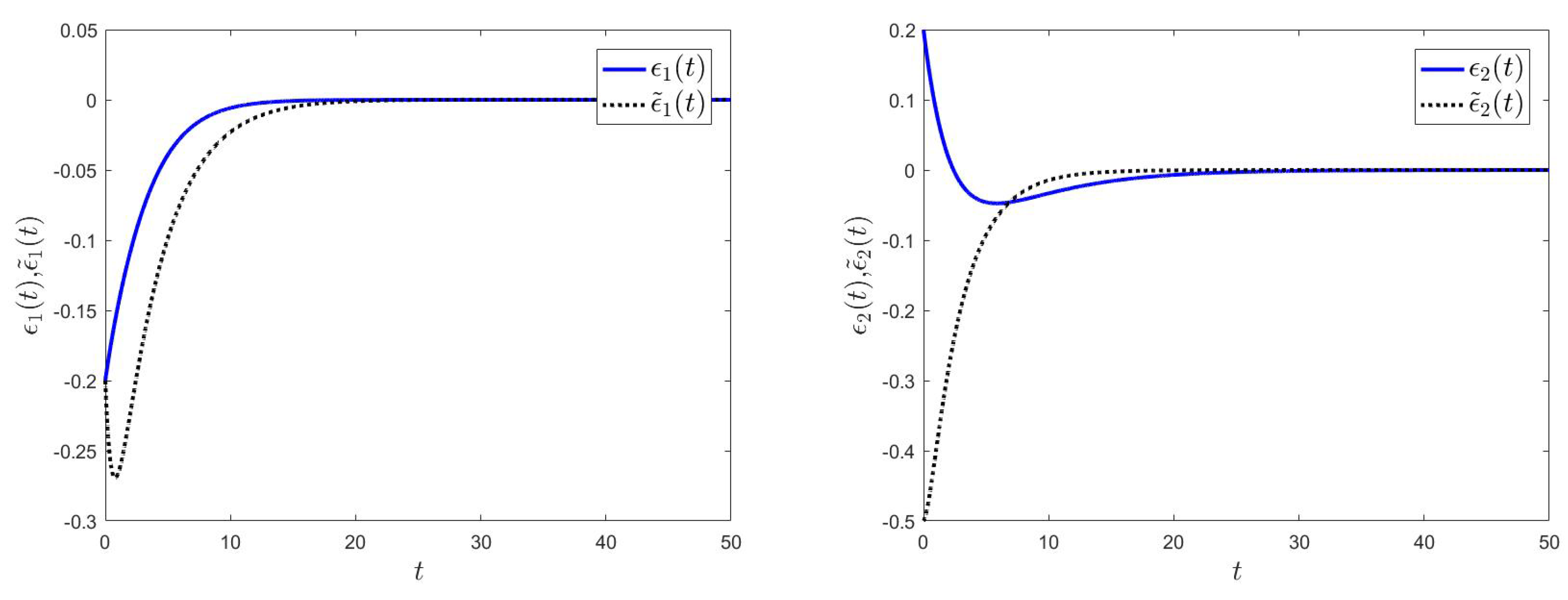
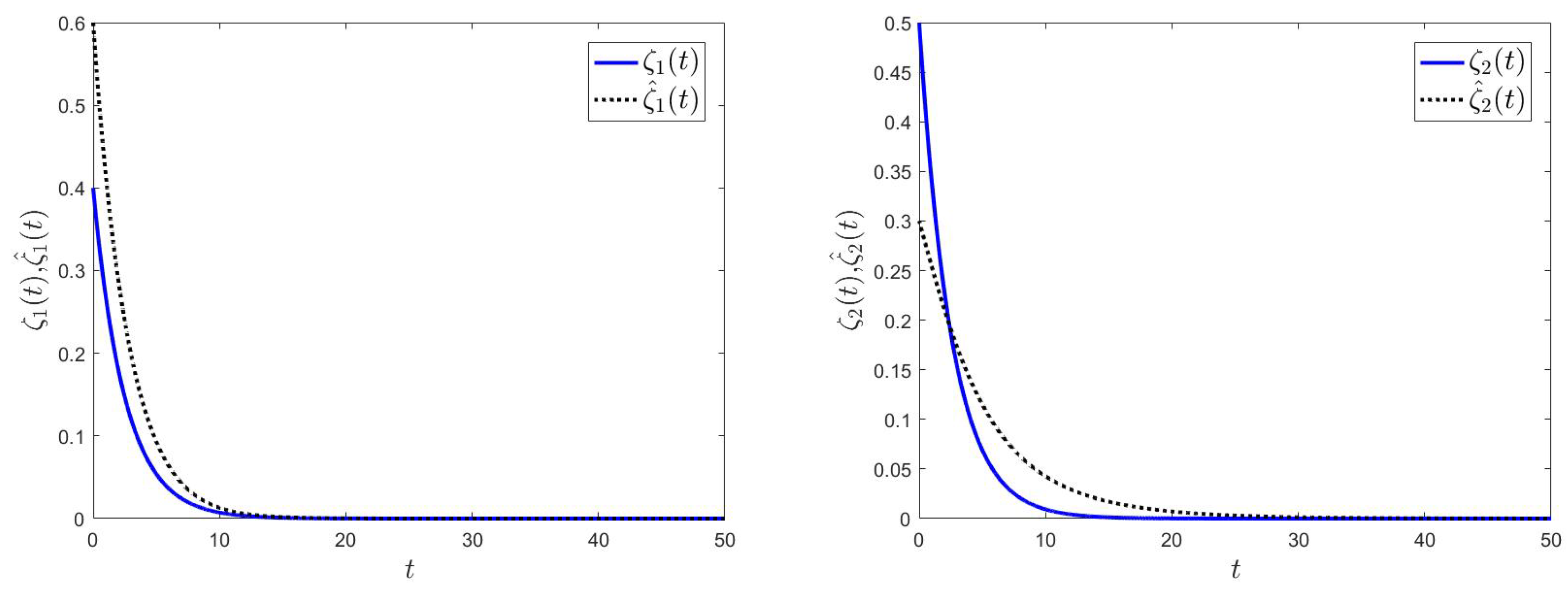
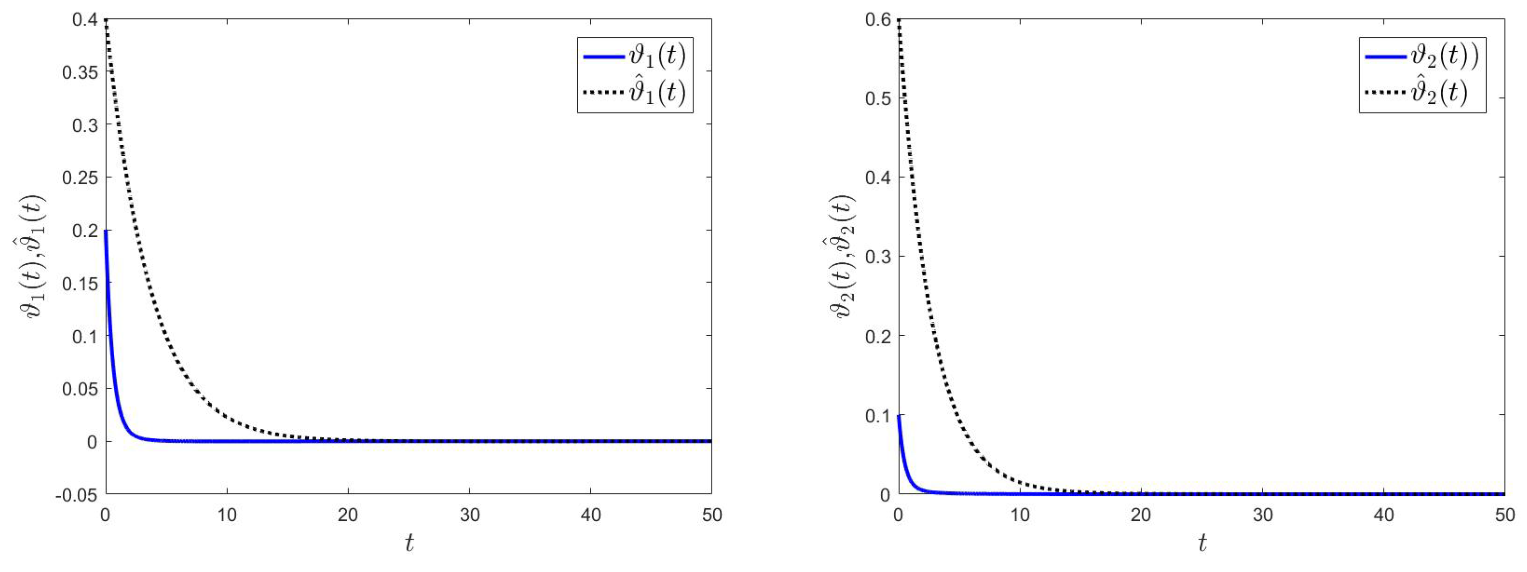
4. Illustrative Examples

Next, the effectiveness of the results given in this paper will be illustrated through a specific numerical example.

Example 1.

Consider drive and response HOBAMNNs (1) and (2) with the controllers in (5): let $n=2$; $m=2$; ${\mathfrak{a}}_1=0.4$; ${\mathfrak{a}}_2=0.4$; ${\widehat{\mathfrak{a}}}_1=0.3$; ${\widehat{\mathfrak{a}}}_2=0.4$; ${\mathfrak{b}}_{11}=1.2$; ${\mathfrak{b}}_{12}=-0.6$; ${\mathfrak{b}}_{21}=-1.3$; ${\mathfrak{b}}_{22}=0.24$; ${\widehat{\mathfrak{b}}}_{11}=1.2; {\widehat{\mathfrak{b}}}_{12}=-0.42; {\widehat{\mathfrak{b}}}_{21}=2.2; {\widehat{\mathfrak{b}}}_{22}=0.22$; ${\mathfrak{c}}_{11}=-1.3; {\mathfrak{c}}_{12}=1.5; g$${\mathfrak{c}}_{21}=2.4$; ${\mathfrak{c}}_{22}=1.1$; ${\widehat{\mathfrak{c}}}_{11}=0.16; {\widehat{\mathfrak{c}}}_{12}=-0.36; {\widehat{\mathfrak{c}}}_{21}=-0.12; {\widehat{\mathfrak{c}}}_{22}=0.43$; ${\mathfrak{d}}_{111}=1; {\mathfrak{d}}_{112}=2; {\mathfrak{d}}_{121}=1$; ${\mathfrak{d}}_{122}=1$; ${\mathfrak{d}}_{211}=2; {\mathfrak{d}}_{212}=1; {\mathfrak{d}}_{221}=1; {\mathfrak{d}}_{222}=0.5$; ${\widehat{\mathfrak{d}}}_{111}=0.1; {\widehat{\mathfrak{d}}}_{112}=0.3; {\widehat{\mathfrak{d}}}_{121}=0.1; {\widehat{\mathfrak{d}}}_{122}=0.3$; ${\widehat{\mathfrak{d}}}_{211}=0.1; {\widehat{\mathfrak{d}}}_{212}=0.21; {\widehat{\mathfrak{d}}}_{221}=0.2; {\widehat{\mathfrak{d}}}_{222}=0.11$; $p_{11}=0.5; p_{12}=0.4; p_{21}=0.2; p_{22}=0.8$; ${\widehat{p}}_{11}=0.7; {\widehat{p}}_{12}=0.1; {\widehat{p}}_{21}=0.2; {\widehat{p}}_{22}=0.9$; $p_{111}=p_{112}=p_{121}=p_{211}=p_{212}=p_{221}=p_{222}=0.8; p_{122}=0.9$; ${\widehat{p}}_{111}={\widehat{p}}_{112}={\widehat{p}}_{121}={\widehat{p}}_{122}=0.8$; ${\widehat{p}}_{211}=0.4; {\widehat{p}}_{212}=0.6$; ${\widehat{p}}_{221}=0.3$; ${\widehat{p}}_{222}=0.7$.

$$h_1\left(s\right)=0.2s{\tanh }^2\left(s\right),h_2\left(s\right)=0.3s{\tanh }^2\left(s\right),$$

$${\tilde{h}}_1\left(s\right)=0.03s{\tanh }^2\left(s\right),{\tilde{h}}_2\left(s\right)=0.2s{\tanh }^2\left(s\right),$$

$$l_1\left(s\right)=0.3s{\tanh }^2\left(s\right),l_2\left(s\right)=0.04s{\tanh }^2\left(s\right),$$

$${\tilde{l}}_1\left(s\right)=0.04s{\tanh }^2\left(s\right),{\tilde{l}}_2\left(s\right)=0.02s{\tanh }^2\left(s\right),$$

$${\hslash }_1\left(s\right)={\hslash }_2\left(s\right)=0.2\tanh \left(s\right),{\tilde{\hslash }}_1\left(s\right)={\tilde{\hslash }}_2\left(s\right)=0.3\tanh \left(s\right),s\in \mathbb{R}.$$

Clearly, set the following: ${\overline{h}}_1=0.2; {\overline{h}}_2=0.3$; ${\overline{\tilde{h}}}_1=0.03; {\overline{\tilde{h}}}_2=0.2$; ${\overline{l}}_1=0.3; {\overline{l}}_2=0.04$; ${\overline{\tilde{l}}}_1=0.04$; ${\overline{\tilde{l}}}_2=0.02$; ${\overline{\hslash }}_1={\overline{\hslash }}_2\left(s\right)=0.2; {\overline{\tilde{\hslash }}}_1={\overline{\tilde{\hslash }}}_2\left(s\right)=0.3$; ${\tilde{\gamma }}_1^{\left(1\right)}={\tilde{\gamma }}_2^{\left(1\right)}=0.2$; ${\tilde{\gamma }}_1^{\left(2\right)}={\tilde{\gamma }}_2^{\left(2\right)}=0.3$. Assumptions 1–4 are satisfied.

When $\lambda =0.05, {\mu }_1=2.6, {\mu }_1=1.6, {\tilde{\mu }}_1=2.0, {\tilde{\mu }}_1=1.8$, ${\eta }_1=2.54, {\eta }_2=1.54,$${\tilde{\eta }}_1=1.94,$ and ${\tilde{\eta }}_2=1.74$, by solving inequalities (7a) and (7b) in Theorem 1, the following feasible solutions are obtained:

$$\tilde{u}={[3.0386,4.3666]}^T,\tilde{v}={[2.4361,2.5156]}^T.$$

It can be readily verified that the conditions of Theorem 1 in our paper are met. Consequently, based on Theorem 1 in our paper, the drive system given by (1) and the response system given by (2) experience semi-global polynomial synchronization under controllers (5). We choose the initial values of the state variables as $\zeta \left(s\right)={[0.4,0.5]}^T$, $\vartheta \left(s\right)={[0.2,0.1]}^T$, $\widehat{\zeta }\left(s\right)={[0.6,0.3]}^T$, and $\widehat{\vartheta }\left(s\right)={[0.4,0.6]}^T$. We also define the external input as $I_1=I_2=0, J_1=J_2=0$. The error curves of drive–response systems ${ϵ}_1\left(t\right),{ϵ}_2\left(t\right),{\widetilde{ϵ}}_1\left(t\right)$, and ${\widetilde{ϵ}}_2\left(t\right)$ are shown in Figure 1; the curves of variables ${\zeta }_1\left(t\right),{\zeta }_2\left(t\right),{\vartheta }_1\left(t\right),{\vartheta }_2\left(t\right)$, ${\widehat{\zeta }}_1\left(t\right),{\widehat{\zeta }}_2\left(t\right),{\widehat{\vartheta }}_1\left(t\right)$, and ${\widehat{\vartheta }}_2\left(t\right)$ are shown in Figure 2 and Figure 3.

Figure 4 and Figure 5, respectively, show the state–response curves corresponding to the time delays of $p_{ijl}={\widehat{p}}_{jir}=0.1$ and $p_{ijl}={\widehat{p}}_{jir}=0.5$, $i,j,r,l\in {\mathbb{Z}}_2$, indicating that different time delays affect the convergence rate of the error system.

5. Conclusions

This paper addresses the issue of SGPS for HOBAMNNs with multiple proportional delays. Utilizing the definition of SGPS, we initially derive delay-dependent SGPS criteria for the error dynamical system. Subsequently, a controller gain is provided. Finally, we present illustrative examples to demonstrate the applicability of the conclusions. Compared with previous research, the main contribution of this work lies in the first investigation of SGPS for HOBAMNNs with multiple proportional delays. By directly deriving easily implementable sufficient criteria based on the definition of SGPS, our approach is applicable to a broader class of NN models. In [47], the general decay synchronization concept for the considered network based on $\psi$-type stability has been given. The general decay synchronization contained polynomial synchronization, exponential synchronization, logarithmic synchronization, and other synchronization as its special cases. We will consider this issue in further research.

References

1. Townsend, J.; Chaton, T.; Monteiro, J.M. Extracting relational explanations from deep neural networks: A survey from a neural-symbolic perspective. IEEE Trans. Neural Netw. Learn. Syst. 2020, 31, 3456–3470. [Google Scholar] [CrossRef] [PubMed]
2. Thangarajan, S.K.; Chokkalingam, A. Integration of optimized neural network and convolutional neural network for automated brain tumor detection. Sens. Rev. 2021, 41, 16–34. [Google Scholar] [CrossRef]
3. Lee, Y.; Doolen, G.; Chen, H.H.; Sun, G.Z.; Maxwell, T.; Lee, H.Y. Machine learning using a higher order correlation network. Phys. D Nonlinear Phenom. 1986, 22, 276–306. [Google Scholar] [CrossRef]
4. Chen, Y.; Zhang, X.; Xue, Y. Global exponential synchronization of high-order quaternion Hopfield neural networks with unbounded distributed delays and time-varying discrete delays. Math. Comput. Simul. 2022, 193, 173–189. [Google Scholar] [CrossRef]
5. Dong, Z.; Wang, X.; Zhang, X.; Hu, M.; Dinh, T.N. Global exponential synchronization of discrete-time high-order switched neural networks and its application to multi-channel audio encryption. Nonlinear Anal. Hybrid Syst. 2023, 47, 101291. [Google Scholar] [CrossRef]
6. Kosko, B. Adaptive bidirectional associative memories. Appl. Opt. 1987, 26, 4947–4960. [Google Scholar] [CrossRef]
7. Kosko, B. Bi-directional associative memories. IEEE Trans. Syst. Man Cybern. 1988, 18, 49–60. [Google Scholar] [CrossRef]
8. Simpson, P.K. Higher-ordered and intraconnected bidirectional associative memories. IEEE Trans. Syst. Man Cybern. Syst. 1990, 20, 637–653. [Google Scholar] [CrossRef]
9. Cao, J.; Liang, J.; Lam, J. Exponential stability of high-order bidirectional associative memory neural networks with time delays. Phys. D Nonlinear Phenom. 2004, 199, 425–436. [Google Scholar] [CrossRef]
10. Aouiti, C.; Li, X.; Miaadi, F. A new LMI approach to finite and fixed time stabilization of high-order class of BAM neural networks with time-varying delays. Neural Process. Lett. 2019, 50, 815–838. [Google Scholar] [CrossRef]
11. Ho, D.W.C.; Liang, J.; Lam, J. Global exponential stability of impulsive high-order BAM neural networks with time-varying delays. Neural Netw. 2006, 19, 1581–1590. [Google Scholar] [CrossRef]
12. Wang, F.; Liu, M. Global exponential stability of high-order bidirectional associative memory (BAM) neural networks with time delays in leakage terms. Neurocomputing 2016, 177, 515–528. [Google Scholar] [CrossRef]
13. Yang, W.; Yu, W.; Cao, J.; Alsaadi, F.E.; Hayat, T. Almost automorphic solution for neutral type high-order Hopfield BAM neural networks with time-varying leakage delays on time scales. Neurocomputing 2017, 267, 241–260. [Google Scholar] [CrossRef]
14. Aouiti, C.; Sakthivel, R.; Touati, F. Global dissipativity of high-order Hopfield bidirectional associative memory neural networks with mixed delays. Neural Comput. Appl. 2020, 32, 10183–10197. [Google Scholar] [CrossRef]
15. Zu, J.; Yu, Z.; Meng, Y. Global exponential stability of high-order bidirectional associative memory (BAM) neural networks with proportional delays. Neural Process. Lett. 2020, 51, 2531–2549. [Google Scholar] [CrossRef]
16. Xing, L.; Zhou, L. Polynomial dissipativity of proportional delayed BAM neural networks. Int. J. Biomath. 2020, 13, 2050050. [Google Scholar] [CrossRef]
17. Zhou, L.; Zhao, Z. Asymptotic stability and polynomial stability of impulsive Cohen–Grossberg neural networks with multi-proportional delays. Neural Process. Lett. 2020, 51, 2607–2627. [Google Scholar] [CrossRef]
18. Wang, Y.; Yang, X.; Chen, X.; Liu, C. Positivity and semi-global polynomial stability of high-order Cohen–Grossberg BAM neural networks with multiple proportional delays. Inf. Sci. 2025, 689, 121512. [Google Scholar] [CrossRef]
19. Pecora, L.M.; Carroll, T.L. Synchronization in chaotic system. Phys. Rev. Lett. 1990, 64, 821–824. [Google Scholar] [CrossRef]
20. Zhou, L. Dissipativity of a class of cellular neural networks with proportional delays. Nonlinear Dyn. 2013, 73, 1895–1903. [Google Scholar] [CrossRef]
21. Jia, S.; Hu, C.; Yu, J.; Jiang, H. Asymptotical and adaptive synchronization of Cohen-Grossberg neural networks with heterogeneous proportional delays. Neurocomputing 2018, 275, 1449–1455. [Google Scholar] [CrossRef]
22. Yang, X.; Song, Q.; Cao, J.; Lu, J. Synchronization of Coupled Markovian Reaction-Diffusion Neural Networks with Proportional Delays via Quantized Control. IEEE Trans. Neural Netw. Learn. Syst. 2019, 30, 951–958. [Google Scholar] [CrossRef]
23. Li, Q.; Zhou, L. Global asymptotic synchronization of inertial memristive Cohen-Grossberg neural networks with proportional delays. Commun. Nonlinear Sci. Numer. Simul. 2023, 123, 107295. [Google Scholar] [CrossRef]
24. Zhou, L. Delay-dependent exponential synchronization of recurrent neural networks with multiple proportional delays. Neural Process. Lett. 2015, 42, 619–632. [Google Scholar] [CrossRef]
25. Wan, P.; Sun, D.; Chen, D.; Zhao, M.; Zheng, L. Exponential synchronization of inertial reaction-diffusion coupled neural networks with proportional delay via periodically intermittent control. Neurocomputing 2019, 356, 195–205. [Google Scholar] [CrossRef]
26. Su, L.; Zhou, L. Exponential synchronization of memristor-based recurrent neural networks with multi-proportional delays. Neural Comput. Appl. 2019, 31, 7907–7920. [Google Scholar] [CrossRef]
27. Li, L.; Chen, W.; Wu, X. Global Exponential Stability and Synchronization for Novel Complex-Valued Neural Networks With Proportional Delays and Inhibitory Factors. IEEE Trans. Cybern. 2021, 51, 2142–2152. [Google Scholar] [CrossRef]
28. Zhang, W.; Li, C.; Huang, T.; Huang, J. Finite-time Synchronization of Neural Networks with Multiple Proportional Delays via Non-chattering Control. Int. J. Control Autom. Syst. 2018, 16, 2473–2479. [Google Scholar] [CrossRef]
29. Xiaolin, X.; Rongqiang, T.; Xinsong, Y. Finite-Time Synchronization of Memristive Neural Networks with Proportional Delay. Neural Process. Lett. 2019, 50, 1139–1152. [Google Scholar]
30. Yang, W.; Huang, J.; He, X.; Wen, S.; Huang, T. Finite-Time Synchronization of Neural Networks With Proportional Delays for RGB-D Image Protection. IEEE Trans. Neural Netw. Learn. Syst. 2024, 35, 8149–8160. [Google Scholar] [CrossRef]
31. Han, J.; Zhou, L. Finite-time synchronization of proportional delay memristive competitive neural networks. Neurocomputing 2024, 610, 128612. [Google Scholar] [CrossRef]
32. Duan, L.; Li, J. Finite-time synchronization for a fully complex-valued BAM inertial neural network with proportional delays via non-reduced order and non-separation approach. Neurocomputing 2025, 611, 128648. [Google Scholar] [CrossRef]
33. Aouiti, C.; Assali, E.A.; Chérif, F.; Zeglaoui, A. Fixed-time synchronization of competitive neural networks with proportional delays and impulsive effect. Neural Comput. Appl. 2020, 32, 13245–13254. [Google Scholar] [CrossRef]
34. Duan, L.; Li, J. Fixed-time synchronization of fuzzy neutral-type BAM memristive inertial neural networks with proportional delays. Inf. Sci. 2021, 576, 522–541. [Google Scholar] [CrossRef]
35. Wan, Y.; Zhou, L. Fixed-time synchronization of discontinuous proportional delay inertial neural networks with uncertain parameters. Inf. Sci. 2024, 678, 120931. [Google Scholar] [CrossRef]
36. Liu, Y.; Wan, X.; Wu, E.; Yang, X.; Alsaadi, F.E.; Hayat, T. Finite-time synchronization of Markovian neural networks with proportional delays and discontinuous activations. Nonlinear Anal. Model. Control 2018, 23, 515–532. [Google Scholar] [CrossRef]
37. Wang, W. Finite-time synchronization for a class of fuzzy cellular neural networks with time-varying coefficients and proportional delays. Fuzzy Sets Syst. 2018, 338, 40–49. [Google Scholar] [CrossRef]
38. Alimi, A.M.; Aouiti, C.; Assali, E.A. Finite-time and fixed-time synchronization of a class of inertial neural networks with multi-proportional delays and its application to secure communication. Neurocomputing 2019, 332, 29–43. [Google Scholar] [CrossRef]
39. Zhang, W.; Li, C.; Yang, S.; Yang, X. Synchronization criteria for neural networks with proportional delays via quantized control. Nonlinear Dyn. 2018, 94, 541–551. [Google Scholar] [CrossRef]
40. Kinh, C.T.; Hien, L.V.; Ke, T.D. Power-Rate Synchronization of Fractional-Order Nonautonomous Neural Networks with Heterogeneous Proportional Delays. Neural Process. Lett. 2018, 47, 139–151. [Google Scholar] [CrossRef]
41. Guan, K. Global power-rate synchronization of chaotic neural networks with proportional delay via impulsive control. Neurocomputing 2018, 283, 256–265. [Google Scholar] [CrossRef]
42. Zhou, L.; Zhao, Z. Exponential synchronization and polynomial synchronization of recurrent neural networks with and without proportional delays. Neurocomputing 2020, 372, 109–116. [Google Scholar] [CrossRef]
43. Yao, Z.; Zhang, Z.; Wang, Z.; Lin, C.; Chen, J. Polynomial synchronization of complex-valued inertial neural networks with multi-proportional delays. Commun. Theor. Phys. 2022, 74, 125801. [Google Scholar] [CrossRef]
44. Zhou, L.; Zhu, Q.; Huang, T. Global Polynomial Synchronization of Proportional Delayed Inertial Neural Networks. IEEE Trans. Syst. Man Cybern. Syst. 2023, 53, 4487–4497. [Google Scholar] [CrossRef]
45. Zhang, J.; Li, Z.; Cao, J.; Abdel-Aty, M.; Meng, X. Polynomial synchronization of quaternion-valued fuzzy cellular neural networks with proportional delays. Nonlinear Dyn. 2025, 113, 3523–3542. [Google Scholar] [CrossRef]
46. Wan, Y.; Zhou, L.; Han, J. Global polynomial synchronization of proportional delay memristive neural networks with uncertain parameters and its application to image encryption. Eng. Appl. Artif. Intell. 2025, 147, 110290. [Google Scholar] [CrossRef]
47. Huang, Y.; Zhao, X. General Decay Synchronization of State and Spatial Diffusion Coupled Delayed Memristive Neural Networks with Reaction-diffusion Terms. Int. J. Control Autom. Syst. 2024, 22, 2313–2326. [Google Scholar] [CrossRef]
Figure 1. The error curves of ϵ ( t ) and ϵ ˜ ( t ) .
Mathematics 13 01512 g001
Figure 2. Synchronization curves of ζ ( t ) and ζ ^ ( t ) .
Mathematics 13 01512 g002
Figure 3. Synchronization curves of ϑ ( t ) and ϑ ^ ( t ) .
Mathematics 13 01512 g003
Figure 4. The error curves of ϵ ( t ) and ϵ ˜ ( t ) when p i j l = p ^ j i r = 0.1 , i , j , r , l Z 2 .
Mathematics 13 01512 g004
Figure 5. The error curves of ϵ ( t ) and ϵ ˜ ( t ) when p i j l = p ^ j i r = 0.5 , i , j , r , l Z 2 .
Mathematics 13 01512 g005
Disclaimer/Publisher’s Note: The statements, opinions and data contained in all publications are solely those of the individual author(s) and contributor(s) and not of MDPI and/or the editor(s). MDPI and/or the editor(s) disclaim responsibility for any injury to people or property resulting from any ideas, methods, instructions or products referred to in the content.