
An Ensemble of Convolutional Neural Networks for Sound Event Detection


Abstract
1. Introduction
1.1. Research Context and Motivation
1.2. Research Aims and Contributions
1.3. Structure of the Paper
2. Related Work
3. Materials and Methods
3.1. Workflow
3.2. Challenges in Sound Event Classification (SED)
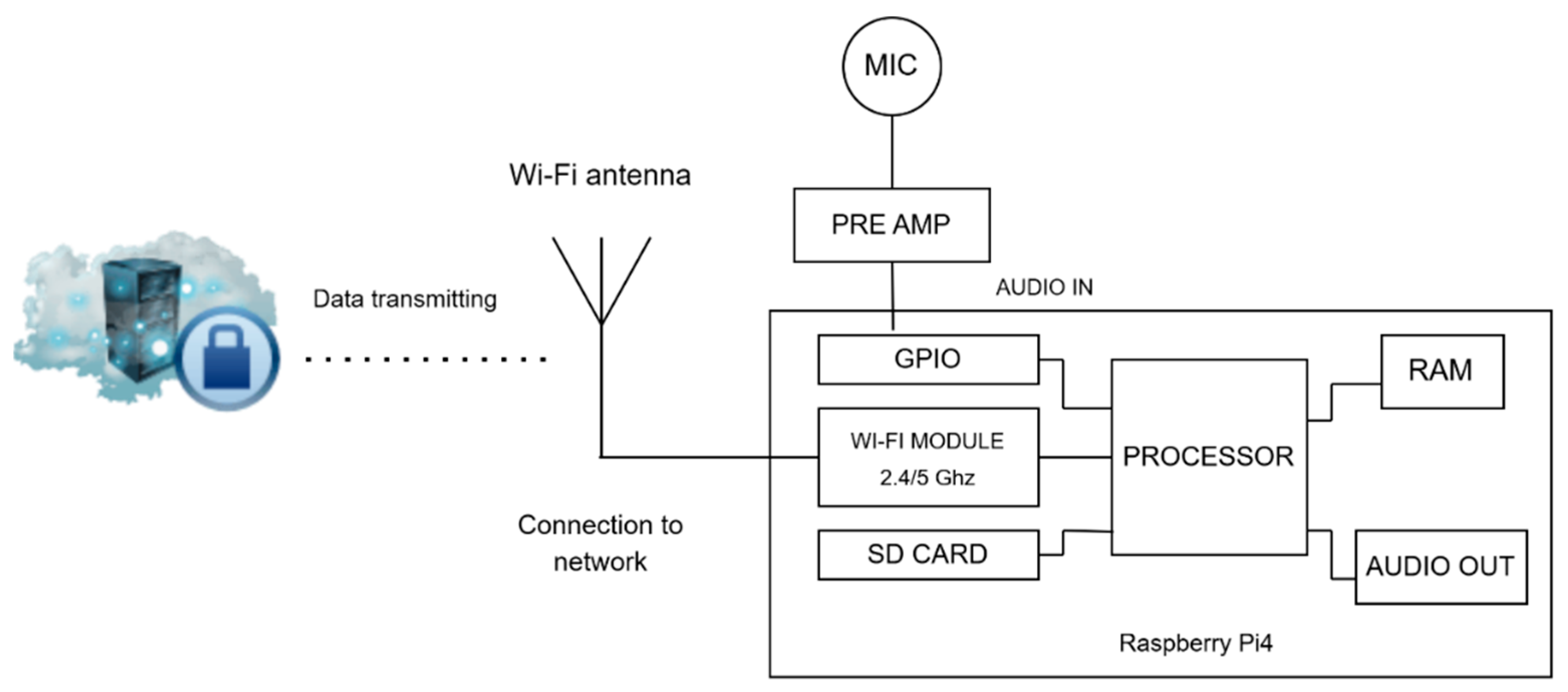
3.3. Data Acquisition
3.3.1. Crowdsourcing
3.3.2. Open Source Datasets
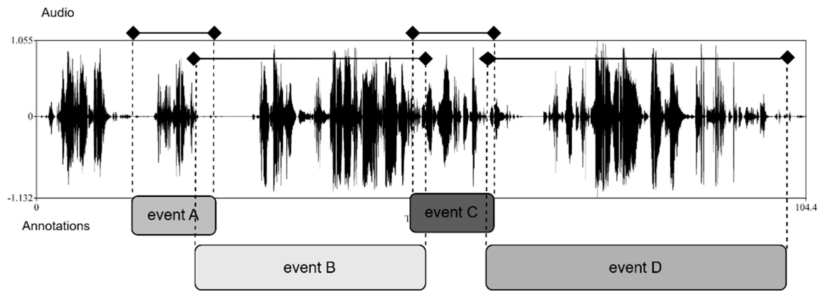
3.4. Data Annotation
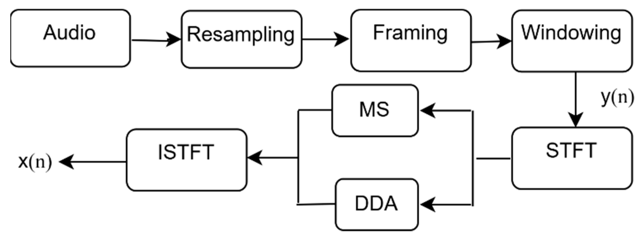
3.5. Pre-Processing
3.6. Feature Extraction
Audio Representations as Images
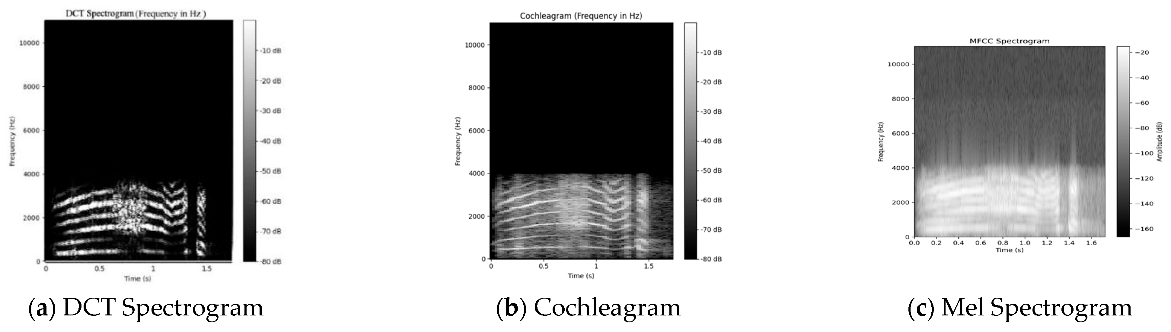
- DCT-based spectrogram: The incoming audio signal has a duration of 2 s (sampling rate, 16 kHz); after going through a framing procedure (frame size = 32 ms, overlap = 50%). the DCT spectral coefficients are calculated for each frame. The formula for the DCT of a 1D signal x[n] is given by
- 2.
- MFCC spectrograms [58]: These spectrograms are derived by computing coefficients that correspond to compositional frequency components, utilizing the short-time Fourier transform (STFT). This extraction process involves applying each frame of the frequency-domain representation to a Mel filter bank. The intensity values of the Mel spectrogram image are calculated using the energy of the filter bank, similar to the MFCCs [12] but without using DCT. The Mel filter bank output of the mth filter can be determined as
- 3.
- Cochleagram: This mapping models the frequency selectivity property of the human cochlea [23,30]. To extract cochlear images from a signal, the incoming signal is first filtered using a gammatone filter bank. The gammatone filter bank is a comb of gammatone filters, each of which is associated with a certain characteristic frequency. The impulse characteristic of a gammatone filter with center frequency fc is described by the expression
4. Data Preparation and Training
4.1. Data Augmentation Techniques
4.2. Dataset
4.2.1. Crowdsourced Dataset
4.2.2. Open Datasets
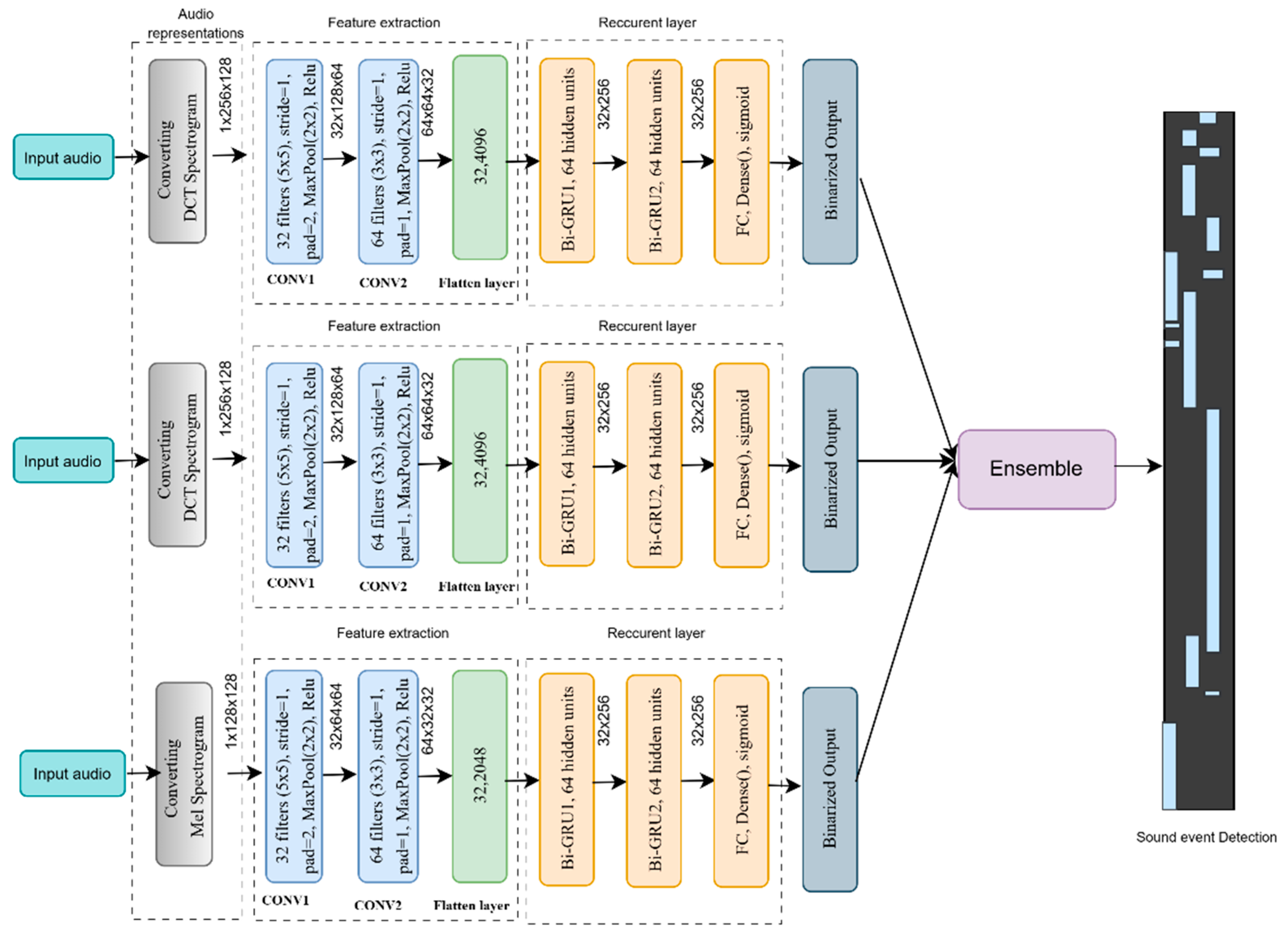
4.3. Development of Ensemble CRNN-Based Model for Sound Event Detection
Convolutional Recurrent Neural Network
4.4. Regularization
4.5. Training
4.6. Metrics
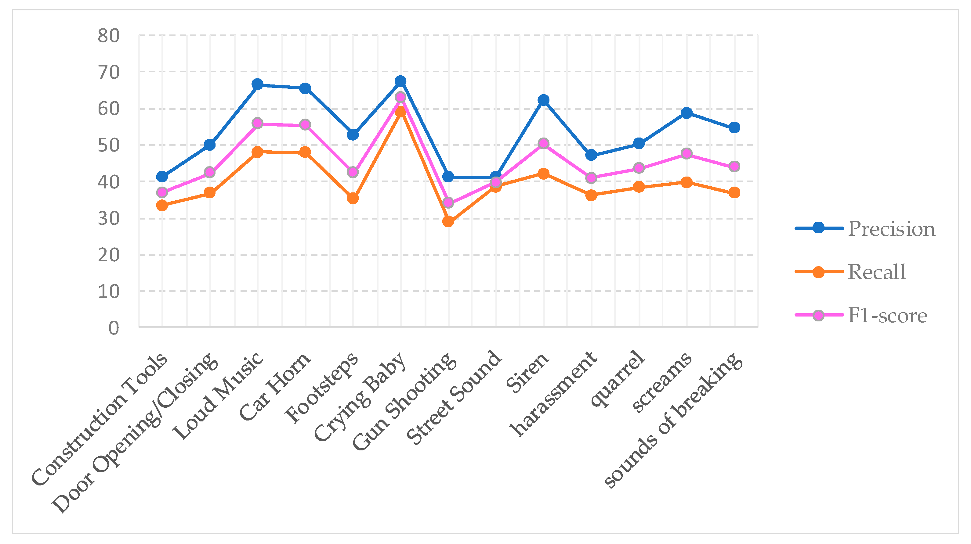
5. Results
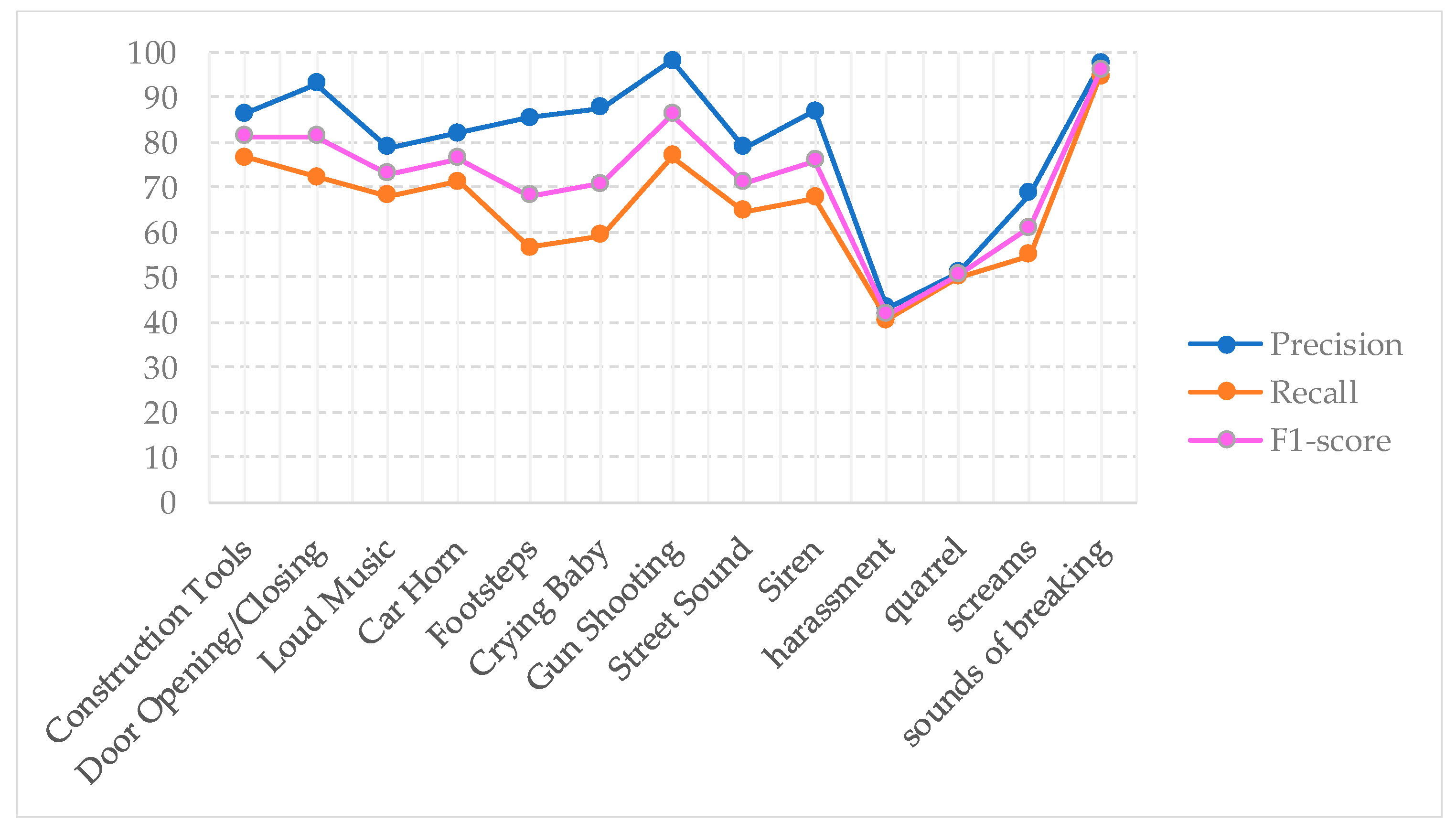
Performance Evaluation
6. Conclusions
Author Contributions
Funding
Informed Consent Statement
Data Availability Statement
Conflicts of Interest
References
- Mukhamadiyev, A.; Khujayarov, I.; Cho, J. Voice-Controlled Intelligent Personal Assistant for Call-Center Automation in the Uzbek Language. Electronics 2023, 12, 4850. [Google Scholar] [CrossRef]
- Musaev, M.; Khujayorov, I.; Ochilov, M. Image Approach to Speech Recognition on CNN. In Proceedings of the 2019 3rd International Symposium on Computer Science and Intelligent Control (ISCSIC 2019), Amsterdam, The Netherlands, 25–27 September 2019; Association for Computing Machinery: New York, NY, USA Article 57. ; pp. 1–6. [Google Scholar] [CrossRef]
- Wang, D.; Brown, G.J. Computational Auditory Scene Analysis: Principles, Algorithms, and Applications; Wiley-IEEE Press: New York, NY, USA, 2006. [Google Scholar]
- Heittola, T.; Mesaros, A.; Virtanen, T.; Gabbouj, M. Supervised model training for overlapping sound events based on unsupervised source separation. In Proceedings of the 2013 IEEE International Conference on Acoustics, Speech and Signal Processing, Vancouver, BC, Canada, 26–31 May 2013; pp. 8677–8681. [Google Scholar] [CrossRef]
- Xu, M.; Xu, C.; Duan, L.; Jin, J.S.; Luo, S. Audio keywords generation for sports video analysis. ACM Trans. Multimed. Comput. Commun. Appl. 2008, 4, 1–23. [Google Scholar] [CrossRef]
- Kim, S.-H.; Nam, H.; Choi, S.-M.; Park, Y.-H. Real-Time Sound Recognition System for Human Care Robot Considering Custom Sound Events. IEEE Access 2024, 12, 42279–42294. [Google Scholar] [CrossRef]
- Neri, M.; Battisti, F.; Neri, A.; Carli, M. Sound Event Detection for Human Safety and Security in Noisy Environments. IEEE Access 2022, 10, 134230–134240. [Google Scholar] [CrossRef]
- Gerosa, L.; Valenzise, G.; Tagliasacchi, M.; Antonacci, F.; Sarti, A. Scream and gunshot detection in noisy environments. In Proceedings of the EURASIP, Poznan, Poland, 3–7 September 2007. [Google Scholar]
- Chu, S.; Narayanan, S.; Kuo, C.-C.J. Environmental sound recognition with time-frequency audio features. IEEE Trans. Audio Speech Lang. Process. 2009, 17, 1142–1158. [Google Scholar] [CrossRef]
- Heittola, T.; Mesaros, A.; Eronen, A.; Virtanen, T. Audio context recognition using audio event histogramsin. In Proceedings of the 18th European Signal Processing Conference, Aalborg, Denmark, 23–27 August 2010; pp. 1272–1276. [Google Scholar]
- Shah, M.; Mears, B.; Chakrabarti, C.; Spanias, A. Lifelogging:archival and retrieval of continuously recorded audio using wearable devices. In Proceedings of the 2012 IEEE International Conference on Emerging Signal Processing Applications (ESPA), Las Vegas, NV, USA, 12–14 January 2012; IEEE Computer Society: Washington, DC, USA, 2012; pp. 99–102. [Google Scholar]
- Wichern, G.; Xue, J.; Thornburg, H.; Mechtley, B.; Spanias, A. Segmentation, indexing, and retrieval for environmental and natural sounds. IEEE Trans. Audio Speech Lang. Process. 2010, 18, 688–707. [Google Scholar] [CrossRef]
- Mukhamadiyev, A.; Khujayarov, I.; Djuraev, O.; Cho, J. Automatic Speech Recognition Method Based on Deep Learning Approaches for Uzbek Language. Sensors 2022, 22, 3683. [Google Scholar] [CrossRef] [PubMed]
- Ochilov, M.M. Using the CTC-based Approach of the End-to-End Model in Speech Recognition. Int. J. Theor. Appl. Issues Digit. Technol. 2023, 3, 135–141. [Google Scholar]
- Adavanne, S.; Parascandolo, G.; Pertila, P.; Heittola, T.; Virtanen, T. Sound event detection in multichannel audio using spatial and harmonic features. In Proceedings of the Workshop on Detection and Classification of Acoustic Scenes Events, Budapest, Hungary, 3 September 2016; pp. 6–10. [Google Scholar]
- Guo, G.; Li, S. Content-based audio classification and retrieval by support vector machines. IEEE Trans. Neural Networks 2003, 14, 209–215. [Google Scholar] [CrossRef]
- Parascandolo, G.; Huttunen, H.; Virtanen, T. Recurrent neural networks for polyphonic sound event detection in real life recordings. In Proceedings of the 2016 IEEE International Conference on Acoustics, Speech and Signal Processing (ICASSP), Shanghai, China, 20–25 March 2016; pp. 6440–6444. [Google Scholar] [CrossRef]
- Bisot, V.; Essid, S.; Richard, G. HOG and subband power distribution image features for acoustic scene classification. In Proceedings of the 23rd European Signal Processing Conference (EUSIPCO), Nice, France, 31 August–4 September 2015; pp. 719–723. [Google Scholar] [CrossRef]
- Rakotomamonjy, A.; Gasso, G. Histogram of Gradients of Time–Frequency Representations for Audio Scene Classification. IEEE/ACM Trans. Audio Speech Lang. Process. 2015, 23, 142–153. [Google Scholar] [CrossRef]
- Çakır, E.; Parascandolo, G.; Heittola, T.; Huttunen, H.; Virtanen, T. Convolutional Recurrent Neural Networks for Polyphonic Sound Event Detection. IEEE/ACM Trans. Audio Speech Lang. Process. 2017, 25, 1291–1303. [Google Scholar] [CrossRef]
- Espi, M.; Fujimoto, M.; Kinoshita, K.; Nakatani, T. Exploiting spectro—Temporal locality in deep learning based acoustic event detection. J. Audio Speech Music Proc. 2015, 2015, 26. [Google Scholar] [CrossRef]
- Auger, F.; Flandrin, P.; Lin, Y.; McLaughlin, S.; Meignen, S.; Oberlin, T.; Wu, H. Time frequency reassignment and synchro squeezing: An overview. IEEE Signal Process. Mag. 2013, 30, 32–41. [Google Scholar] [CrossRef]
- Sharan, R.V.; Moir, T.J. Cochleagram image feature for improved robustness in sound recognition. In Proceedings of the 2015 IEEE International Conference on Digital Signal Processing (DSP), Singapore, 21–24 July 2015; pp. 441–444. [Google Scholar] [CrossRef]
- Dennis, J.; Tran, H.D.; Chng, E.S. Analysis of spectrogram image methods for sound event classification. In Proceedings of the Interspeech, Singapore, 14–18 September 2014. [Google Scholar]
- Spadini, T.; de Oliveira Silva, D.L.; Suyama, R. Sound event recognition in a smart city surveillance context. arXiv 2019, arXiv:1910.12369. [Google Scholar]
- Ciaburro, G.; Iannace, G. Improving Smart Cities Safety Using Sound Events Detection Based on Deep Neural Network Algorithms. Informatics 2020, 7, 23. [Google Scholar] [CrossRef]
- Ranmal, D.; Ranasinghe, P.; Paranayapa, T.; Meedeniya, D.; Perera, C. ESC-NAS: Environment Sound Classification Using Hardware-Aware Neural Architecture Search for the Edge. Sensors 2024, 24, 3749. [Google Scholar] [CrossRef]
- Zhang, H.; McLoughlin, I.; Song, Y. Robust sound event recognition using convolutional neural networks. In Proceedings of the 2015 IEEE International Conference on Acoustics, Speech and Signal Processing (ICASSP), South Brisbane, QLD, Australia, 19–24 April 2015; pp. 559–563. [Google Scholar] [CrossRef]
- Kwak, J.-Y.; Chung, Y.-J. Sound Event Detection Using Derivative Features in Deep Neural Networks. Appl. Sci. 2020, 10, 4911. [Google Scholar] [CrossRef]
- Nanni, L.; Maguolo, G.; Brahnam, S.; Paci, M. An Ensemble of Convolutional Neural Networks for Audio Classification. Appl. Sci. 2021, 11, 5796. [Google Scholar] [CrossRef]
- Xiong, W.; Xu, X.; Chen, L.; Yang, J. Sound-Based Construction Activity Monitoring with Deep Learning. Buildings 2022, 12, 1947. [Google Scholar] [CrossRef]
- Sharan, R.V.; Moir, T.J. Acoustic event recognition using cochleagram image and convolutional neural networks. Appl. Acoust. 2019, 148, 62–66. [Google Scholar] [CrossRef]
- Heittola, T.; Mesaros, A.; Eronen, A.; Virtanen, T. Context-dependent sound event detection. EURASIP J. Audio Speech Music. Process. 2013, 2013, 1. [Google Scholar] [CrossRef]
- Zheng, X.; Zhang, C.; Chen, P.; Zhao, K.; Jiang, H.; Jiang, Z.; Pan, H.; Wang, Z.; Jia, W. A CRNN System for Sound Event Detection Based on Gastrointestinal Sound Dataset Collected by Wearable Auscultation Devices. IEEE Access 2020, 8, 157892–157905. [Google Scholar] [CrossRef]
- Lim, W.; Suh, S.; Park, S.; Jeong, Y. Sound Event Detection in Domestic Environments Using Ensemble of Convolutional Recurrent Neural Networks. In Proc. Detection Classification Acoust. Scenes Events Workshop. 2019. June. Available online: https://dcase.community/documents/challenge2019/technical_reports/DCASE2019_Lim_77.pdf (accessed on 10 April 2025).
- Arslan, Y.; Canbolat, H. Performance of Deep Neural Networks in Audio Surveillance. In Proceedings of the IEEE 2018 6th International Conference on Control Engineering & Information Technology (CEIT), Istanbul, Turkey, 25–27 October 2018; pp. 1–5. [Google Scholar] [CrossRef]
- Kang, J.; Lee, S.; Lee, Y. DCASE 2022 Challenge Task 3: Sound event detection with target sound augmentation. DCASE 2022 Community.
- Gygi, B.; Shafiro, V. Environmental sound research as it stands today. Proc. Meetings Acoust. 2007, 1, 050002. [Google Scholar]
- Salamon, J.; Jacoby, C.; Bello, J.P. A Dataset and Taxonomy for Urban Sound Research. In Proceedings of the 22nd ACM International Conference on Multimedia (MM ‘14), Orlando, FL, USA, 3–7 November 2014; pp. 1041–1044. [Google Scholar] [CrossRef]
- Gemmeke, J.F.; Ellis, D.P.; Freedman, D.; Jansen, A.; Lawrence, W.; Moore, R.C.; Plakal, M.; Ritter, M. Audio Set: An ontology and human-labeled dataset for audio events. In Proceedings of the 2017 IEEE International Conference on Acoustics, Speech and Signal Processing (ICASSP), New Orleans, LA, USA, 5–9 March 2017; pp. 776–780. [Google Scholar]
- Fonseca, E.; Favory, X.; Pons, J.; Font, F.; Serra, X. FSD50K: An Open Dataset of Human-Labeled Sound Events. IEEE/ACM Trans. Audio Speech Lang. Process 2022, 30, 829–852. [Google Scholar] [CrossRef]
- Mesaros, A.; Heittola, T.; Virtanen, T. TUT database for acoustic scene classification and sound event detection. In Proceedings of the 24th European Signal Processing Conference (EUSIPCO), Budapest, Hungary, 29 August–2 September 2016; pp. 1128–1132. [Google Scholar] [CrossRef]
- Piczak, K.J. ESC: Dataset for Environmental Sound Classification. In Proceedings of the 23rd ACM International Conference on Multimedia (MM ’15), Brisbane, Australia, 26–30 October 2015; Association for Computing Machinery: New York, NY, USA; pp. 1015–1018. [Google Scholar] [CrossRef]
- Fillon, T.; Simonnot, J.; Mifune, M.-F.; Khoury, S.; Pellerin, G.; Le Coz, M. Telemeta: An open-source web framework for ethnomusicological audio archives management and automatic analysis. In Proceedings of the 1st International Workshop on Digital Libraries for Musicology (DLfM 2014), London, UK; 12 September 2014, pp. 1–8.
- Mesaros, A.; Heittola, T.; Virtanen, T.; Plumbley, M.D. Sound Event Detection: A tutorial. IEEE Signal Process. Mag. 2021, 38, 67–83. [Google Scholar] [CrossRef]
- Kim, B.; Pardo, B. I-SED: An Interactive Sound Event Detector. In Proceedings of the 22nd International Conference on Intelligent User Interfaces (IUI ‘17), Limassol, Cyprus, 13–16 March 2017; Association for Computing Machinery: New York, NY, USA; pp. 553–557. [Google Scholar] [CrossRef]
- Queensland University of Technology’s Ecoacoustics Research Group. Bioacoustics Workbench. 2017. Available online: https://github.com/QutBioacoustics/baw-client (accessed on 10 April 2025).
- Katspaugh. 2017. wavesurfer.js. Available online: https://wavesurfer-js.org/ (accessed on 10 April 2025).
- Cartwright, M.; Seals, A.; Salamon, J.; Williams, A.; Mikloska, S.; MacConnell, D.; Law, E.; Bello, J.; Nov, O. Seeing sound: Investigating the effects of visualizations and complexity on crowdsourced audio annotations. In Proceedings of the ACM on Human-Computer Interaction, Denver, CO, USA, 6–11 May 2017. [Google Scholar]
- Martin, R. Noise power spectral density estimation based on optimal smoothing and minimum statistics. IEEE Trans. Speech Audio Process. 2001, 9, 504–512. [Google Scholar] [CrossRef]
- The Audio Annotation Tool for Your AI. SuperAnnotate. Available online: https://www.superannotate.com/audio-annotation (accessed on 10 April 2025).
- Heittola, T.; Çakır, E.; Virtanen, T. The Machine Learning Approach for Analysis of Sound Scenes and Events. In Computational Analysis of Sound Scenes and Events; Virtanen, T., Plumbley, M., Ellis, D., Eds.; Springer: Cham, Switzerland, 2017. [Google Scholar] [CrossRef]
- Bo, H.; Li, H.; Ma, L.; Yu, B. A Constant Q Transform based approach for robust EEG spectral analysis. In Proceedings of the 2014 International Conference on Audio, Language and Image Processing, Shanghai, China, 7–9 July 2014; pp. 58–63. [Google Scholar] [CrossRef]
- Musaev, M.; Mussakhojayeva, S.; Khujayorov, I.; Khassanov, Y.; Ochilov, M.; Atakan Varol, H. USC: An Open-Source Uzbek Speech Corpus and Initial Speech Recognition Experiments. In Speech and Computer, Proceedings of the Speech and Computer (SPECOM 2021), St. Petersburg, Russia, 27–30 September 2021; Karpov, A., Potapova, R., Eds.; Lecture Notes in Computer Science; Springer: Cham, Switzerland, 2021; Volume 12997. [Google Scholar] [CrossRef]
- Musaev, M.; Khujayorov, I.; Ochilov, M. Automatic Recognition of Uzbek Speech Based on Integrated Neural Networks. In Advances in Intelligent Systems and Computing, Proceeding of the 11th World Conference “Intelligent System for Industrial Automation” (WCIS-2020), Tashkent, Uzbekistan, 26–28 November 2020; Aliev, R.A., Yusupbekov, N.R., Kacprzyk, J., Pedrycz, W., Sadikoglu, F.M., Eds.; Springer: Cham, Switzerland, 2021; Volume 1323. [Google Scholar] [CrossRef]
- Tzanetakis, G.; Essl, G.; Cook, P.R. Audio analysis using the discrete wavelet transform. In Proceedings of the Acoustics and Music Theory Applications; Citeseer: Princeton, NJ, USA, 2001; Volume 66, pp. 318–323. [Google Scholar]
- Available online: https://brianmcfee.net/dstbook-site/content/ch09-stft/Framing.html (accessed on 10 April 2025).
- Rabiner, L.R.; Schafer, R.W. Theory and Applications of Digital Speech Processing; Prentice Hall Press: Hoboken, NJ, USA, 2010. [Google Scholar]
- Porkhun, M.I.; Vashkevich, M.I. Efficient implementation of gammatone filters based on unequal-band cosine-modulated filter bank. Comput. Sci. Autom. 2024, 23, 1398–1422. [Google Scholar] [CrossRef]
- Cui, X.; Goel, V.; Kingsbury, B. Data augmentation for deep neural network acoustic modeling. IEEE/ACM Trans. Audio Speech Lang. Process. 2015, 23, 1469–1477. [Google Scholar]
- Jaitly, N.; Hinton, G.E. Vocal tract length perturbation (VTLP) improves speech recognition. In Proceedings of the ICML Workshop on Deep Learning for Audio, Speech and Language, Atlanta, GA, USA, 16–21 June 2013. [Google Scholar]
- McFee, B.; Humphrey, E.J.; Bello, J.P. A software framework for musical data augmentation. In Proceedings of the International Society for Music Information Retrieval Conference (ISMIR), Málaga, Spain, 26–30 October 2015. [Google Scholar]
- Ko, T.; Peddinti, V.; Povey, D.; Khudanpur, S. Audio augmentation for speech recognition. In Proceedings of the Interspeech, Dresden, Germany, 6–10 September 2015. [Google Scholar]
- Srivastava, N.; Hinton, G.E.; Krizhevsky, A.; Sutskever, I.; Salakhutdinov, R. Dropout: A simple way to prevent neural networks from overfitting. J. Mach. Learn. Res. 2014, 15, 1929–1958. [Google Scholar]
- Gal, Y.; Ghahramani, Z. A theoretically grounded application of dropout in recurrent neural networks. In Proceedings of the 30th International Conference on Neural Information Processing Systems, Barcelona, Spain, 5–10 December 2016. [Google Scholar]
- Ioffe, S.; Szegedy, C. Batch Normalization: Accelerating Deep Network Training by Reducing Internal Covariate Shift. arXiv 2015, arXiv:1502.03167v3Search. [Google Scholar]
- Santos, C.F.G.D.; Papa, J.P. Avoiding Overfitting: A Survey on Regularization Methods for Convolutional Neural Networks. ACM Comput. Surv. 2022, 54, 1–25. [Google Scholar] [CrossRef]
- Salehin, I.; Kang, D.-K. A Review on Dropout Regularization Approaches for Deep Neural Networks within the Scholarly Domain. Electronics 2023, 12, 3106. [Google Scholar] [CrossRef]
- Szymański, P.; Kajdanowicz, T. A Network Perspective on Stratification of Multi-Label Data. arXiv 2017, arXiv:1704.08756v1. [Google Scholar]
- Mesaros, A.; Heittola, T.; Virtanen, T. Metrics for Polyphonic Sound Event Detection. Appl. Sci. 2016, 6, 162. [Google Scholar] [CrossRef]
- Wei, W.; Zhu, H.; Emmanouil, B.; Wang, Y. A-CRNN: A Domain Adaptation Model for Sound Event Detection. In Proceedings of the 2020 IEEE International Conference on Acoustics, Speech and Signal Processing (ICASSP), Barcelona, Spain, 4–8 May 2020; pp. 276–280. [Google Scholar] [CrossRef]


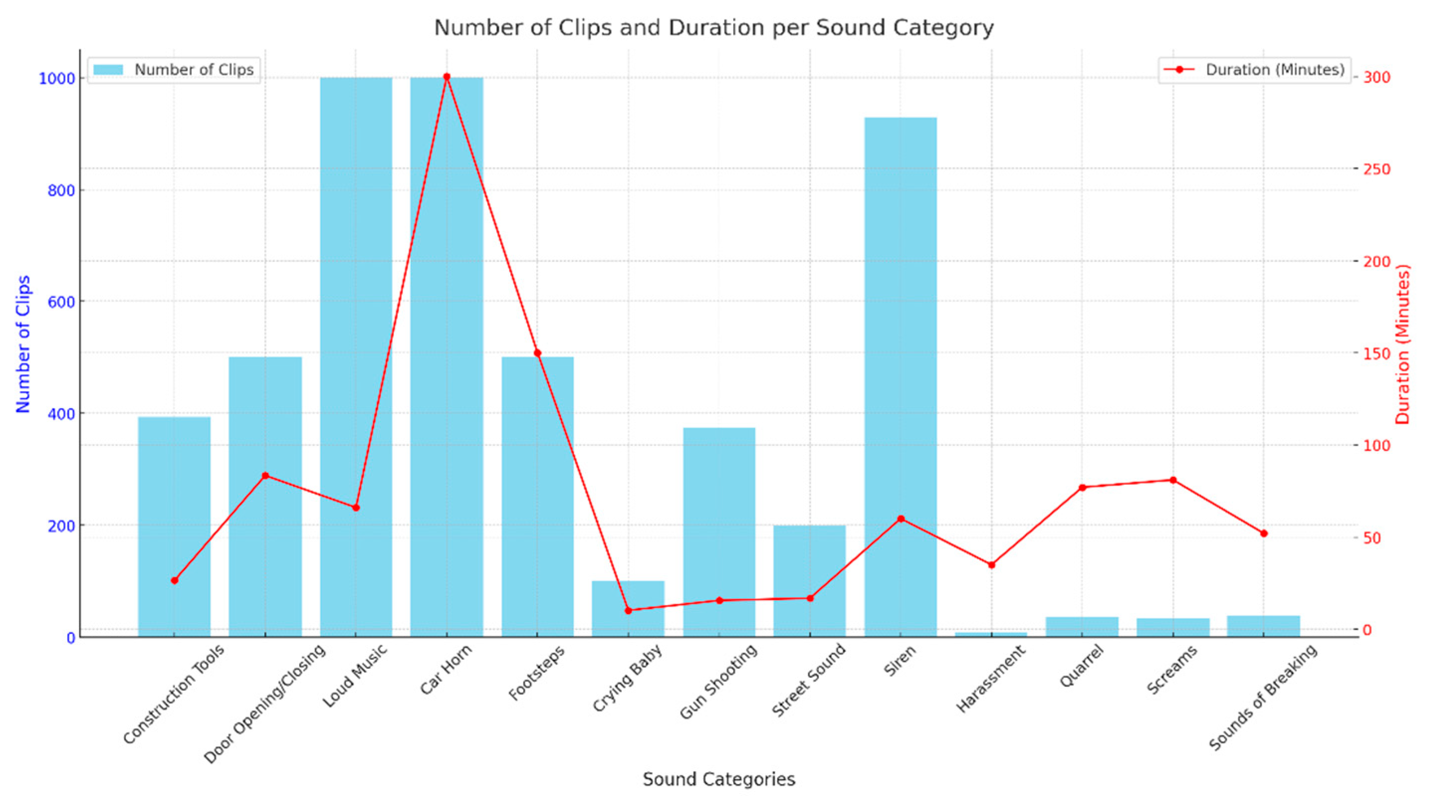
| Harassment | Quarrel | Screams | Sounds of Breaking | |
|---|---|---|---|---|
| Number of clips | 6 | 36 | 33 | 37 |
| Duration (minutes) | 35 | 77 | 81 | 52 |
| Sound Class | Datasets | Number of Clips | Average Duration (Seconds) | Sample Rate |
|---|---|---|---|---|
| Construction Tools | UrbanSound8K | ~394 | ~4.0 | 44.1 kHz |
| Door Opening/Closing | AudioSet Ontology | ~500+ | ~10 | |
| Loud Music | UrbanSound8K | ~1000 | ~3.5 | |
| Car Horn | AudioSet Ontology | ~1000+ | Varies (5–30) | |
| Footsteps | FSD50K | ~500+ | Varies (5–30) | |
| Crying Baby | ESC-50 | ~100+ | ~5.0 | |
| Gun Shooting | UrbanSound8K | 374 | ~2.5 | |
| Street Sound | TUT Sound Events 2017 | ~200 | ~5.0 | 48 kHz |
| Siren | UrbanSound8K | ~929 | ~3.7 | 44.1 kHz |
| Sound Category | Total (Minutes) | Train (80%) | Validation (10%) | Test (10%) | Source |
|---|---|---|---|---|---|
| Construction Tools | 26.4 | 21.12 | 2.64 | 2.64 | Open source |
| Door Opening/Closing | 83.4 | 66.72 | 8.34 | 8.34 | |
| Loud Music | 66 | 52.80 | 6.60 | 6.60 | |
| Car Horn | 300 | 240 | 30 | 30 | |
| Footsteps | 150 | 120 | 15 | 15 | |
| Crying Baby | 10.2 | 8.16 | 1.02 | 1.02 | |
| Gun Shooting | 15.6 | 12.48 | 1.56 | 1.56 | |
| Street Sound | 16.8 | 13.44 | 1.68 | 1.68 | |
| Siren | 60 | 48.00 | 6.00 | 6.00 | |
| Harassment | 35 | 28.0 | 3.50 | 3.50 | Crowdsourcing |
| Quarrel | 77 | 61.60 | 7.70 | 7.70 | |
| Screams | 81 | 64.80 | 8.10 | 8.10 | |
| Sounds of Breaking | 52 | 41.60 | 5.20 | 5.20 |
| Layers | Hyperparameters | |
|---|---|---|
| DCT and Cochleagram Spectrogram | Mel spectrogram | |
| Input | ||
| Conv1 | 32 filters, 5 5, stride = 1, pad = 2, ReLU | 32 filters, 5 5, stride = 1, pad = 2, ReLU |
| Pool1 | MaxPool 2 2 | MaxPool 2 2 |
| Conv2 | 64 filters, 3 3, stride = 1, pad = 1, ReLU | 64 filters, 3 3, stride = 1, pad = 1, ReLU |
| Pool2 | MaxPool 2 2 | MaxPool 2 2 |
| Reshape | (B, 64, 64, 32) (B, 32, 64 64 = 4096) | (B, Time = 32, 64 32 = 2048) |
| Bi-GRU1 | 64 hidden units | 64 hidden units |
| Bi-GRU2 | 64 hidden units | 64 hidden units |
| Dropout (Conv +RNN) | 0.3 in Conv blocks and GRU layers | 0.2 in Conv blocks and GRU layers |
| Dense | Number of sound events, sigmoid | Number of sound events, sigmoid |
| Loss Function | Binary cross-entropy (multi-label) | |
| Optimizer | Adam | |
| Learning rate | ||
| Batch normalization | 32 | |
| Number of training | 50 | |
| Ensemble Method | Vote over model outputs | |
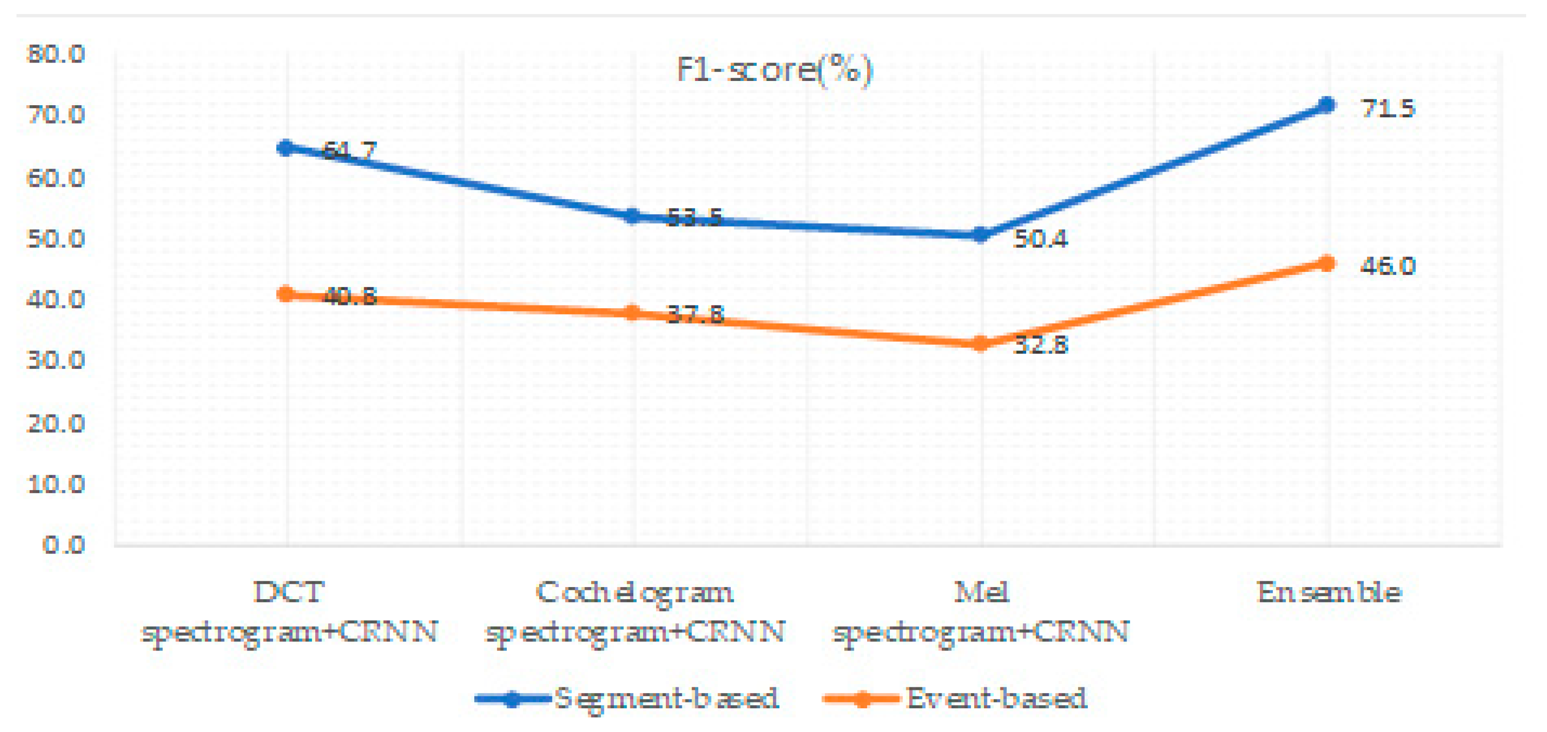
| F1-Score(%) | Error Rate | |||
|---|---|---|---|---|
| Methods | Segment-Based | Event-Based | Segment-Based | Event-Based |
| DCT spectrogram + CRNN | 64.7 | 40.8 | 0.74 | 0.84 |
| Cochelogram spectrogram + CRNN | 53.5 | 37.8 | 1 | 1 |
| Mel spectrogram + CRNN | 50.4 | 32.8 | 0.97 | 1.2 |
| Ensemble | 71.5 | 46.0 | 0.92 | 1.1 |
| Authors | Model | Dataset | Classes | Key Features | F1 Score (Segment/Event) | Application |
|---|---|---|---|---|---|---|
| Yüksel Arslan et al. (2018) [36] | DNN | Custom | 2 | MFCC | F-score 75.4% | Urban safety |
| Xue Zheng et al. (2020) [34] | CRNN (LSTM) | GI Sound set | 6 | MFCC | 81.06%/- | Medical monitoring |
| Emre Çakır et al. (2017) [20] | Single CRNN (GRU) | TUT-SED Synthetic 2016 | 16 | MFCC | F1frame = 66.4%, F1sec = 68.7% | General polyphonic SED |
| Wuyue Xiong et al. (2022) [31] | CRNN (GRU) | Custom | 5 | Mel spectrogram | 82% (accuracy)/- | Construction monitoring |
| Sang-Ick Kang et al. (2022) [37] | CRNN ensemble | DCASE 2022 SELD Synthetic dataset | 12 | Mel spectrogram | 53%/- | Polyphonic SED + location |
| Wei Wei et al. (2020) [71] | Adapted CRNN | DCASE | 5 | MFCC | 51.4%/- | Domestic SED |
| Wootaek Lim et al. (2019) [35] | CRNN (Bi-GRU) | DCASE 2019 | 10 | Mel spectrogram | 66.17%/40.89% | Domestic SED |
| Ours (2025) | CRNN (LSTM) ensemble | Crowdsourced and Open source | 13 | DCT, Mel, Cochleagram spectrograms | 71.5%/46% | Urban safety |
Disclaimer/Publisher’s Note: The statements, opinions and data contained in all publications are solely those of the individual author(s) and contributor(s) and not of MDPI and/or the editor(s). MDPI and/or the editor(s) disclaim responsibility for any injury to people or property resulting from any ideas, methods, instructions or products referred to in the content. |
© 2025 by the authors. Licensee MDPI, Basel, Switzerland. This article is an open access article distributed under the terms and conditions of the Creative Commons Attribution (CC BY) license (https://creativecommons.org/licenses/by/4.0/).
Share and Cite
Mukhamadiyev, A.; Khujayarov, I.; Nabieva, D.; Cho, J. An Ensemble of Convolutional Neural Networks for Sound Event Detection. Mathematics 2025, 13, 1502. https://doi.org/10.3390/math13091502
Mukhamadiyev A, Khujayarov I, Nabieva D, Cho J. An Ensemble of Convolutional Neural Networks for Sound Event Detection. Mathematics. 2025; 13(9):1502. https://doi.org/10.3390/math13091502
Chicago/Turabian StyleMukhamadiyev, Abdinabi, Ilyos Khujayarov, Dilorom Nabieva, and Jinsoo Cho. 2025. "An Ensemble of Convolutional Neural Networks for Sound Event Detection" Mathematics 13, no. 9: 1502. https://doi.org/10.3390/math13091502
APA StyleMukhamadiyev, A., Khujayarov, I., Nabieva, D., & Cho, J. (2025). An Ensemble of Convolutional Neural Networks for Sound Event Detection. Mathematics, 13(9), 1502. https://doi.org/10.3390/math13091502