Figure 1.
Metaheuristic classification.
Figure 1.
Metaheuristic classification.
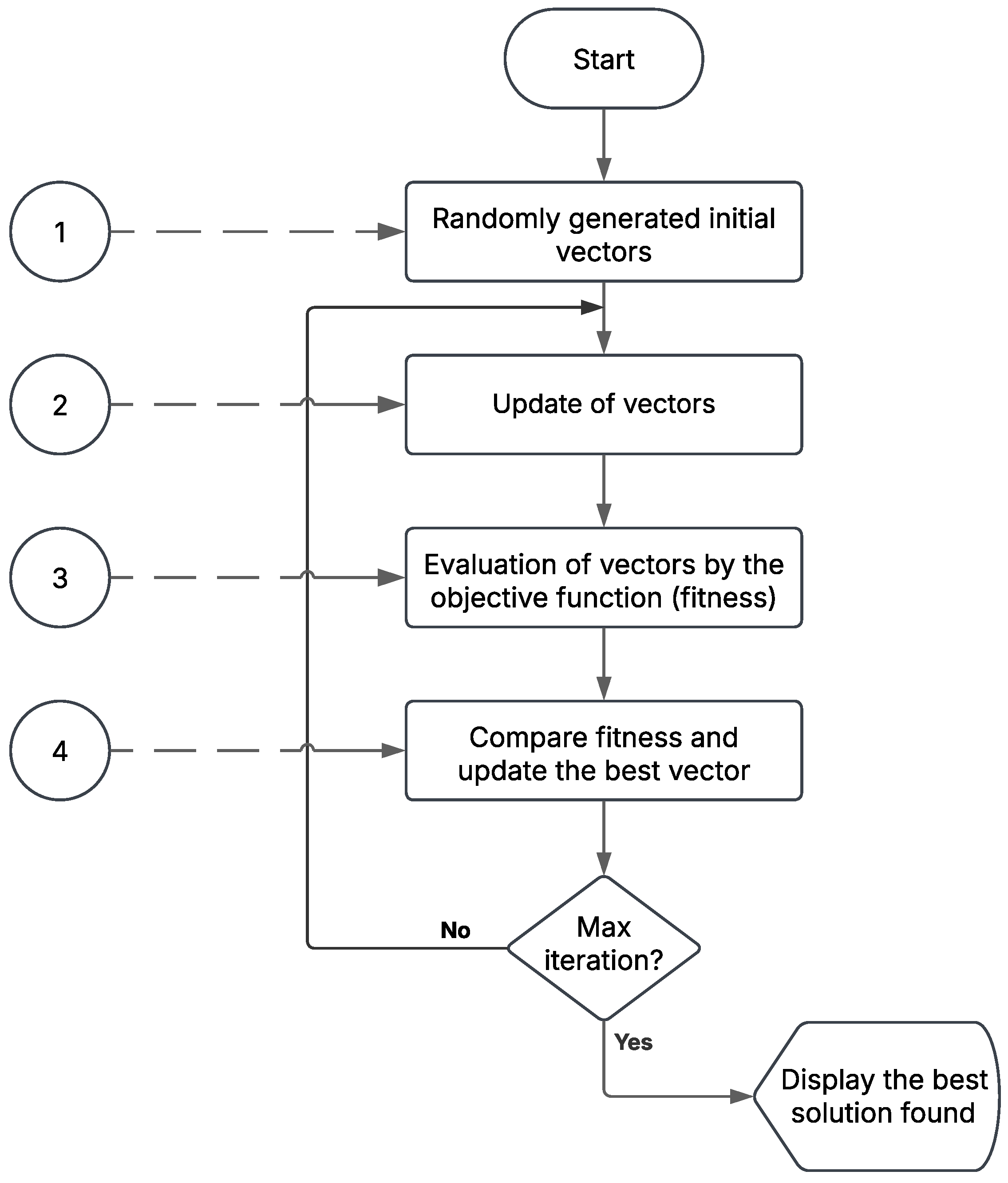
Figure 2.
Schematic representation of a metaheuristic algorithm.
Figure 2.
Schematic representation of a metaheuristic algorithm.
Figure 3.
(a) The shrimp inside its shelter. Photograph (published under a CC BY license). Author unknown. (b) The shrimp observing in different directions simultaneously. Photograph (published under a CC BY-SA license). Author unknown. (c) The purple-spotted mantis shrimp (Gonodactylus smithii). Photograph by Roy L. Caldwell (published under a CC BY-SA license). (d) Strike of a mantis shrimp. Photograph (published under a CC BY license). Author unknown.
Figure 4.
Shrimp strategies based on detected polarized light.
Figure 4.
Shrimp strategies based on detected polarized light.
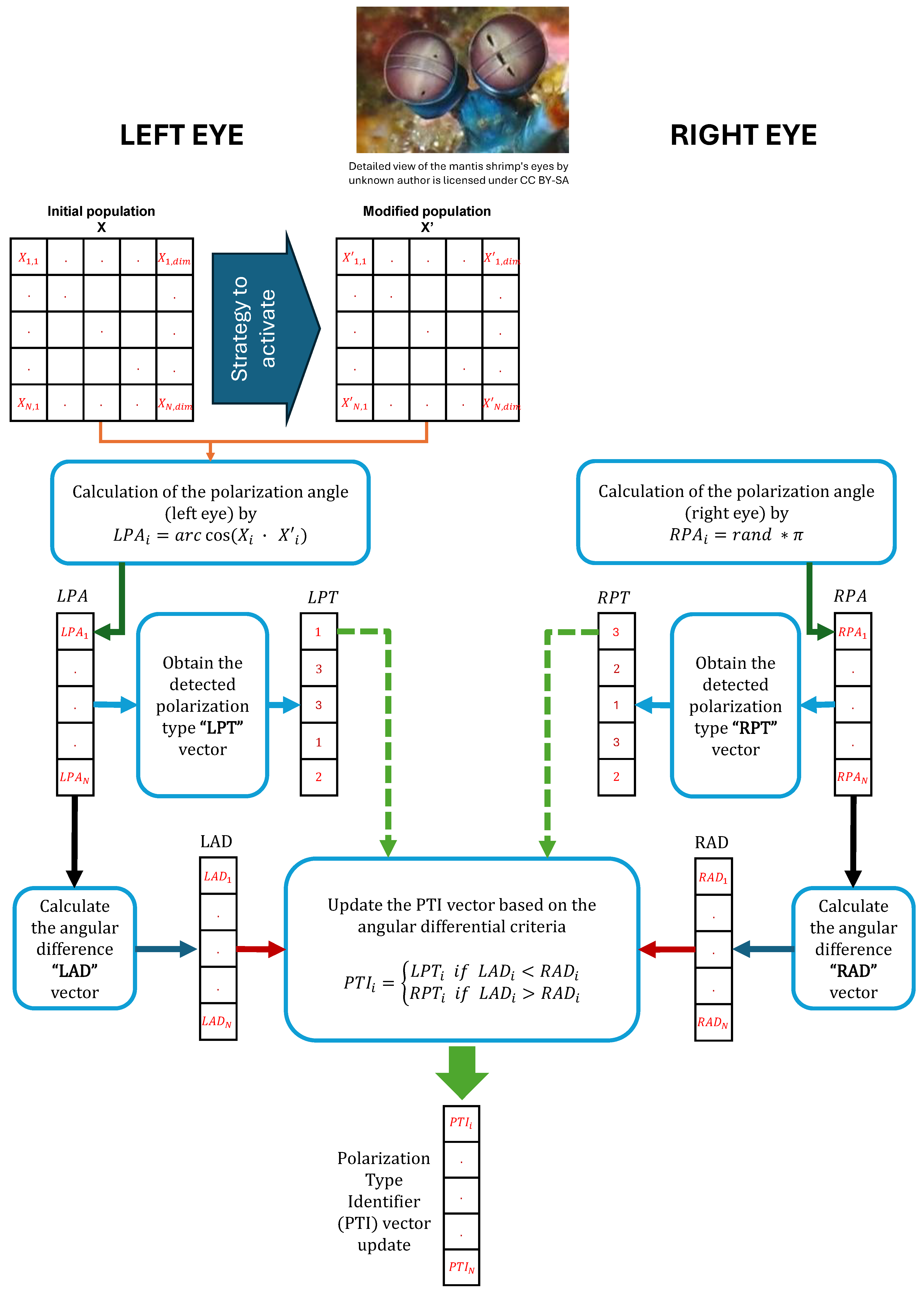
Figure 5.
(a) Schematic representation of the initial population, where stands for the vector size; (b) Polarization Type Identifier (PTI) vector representation; (c) strategy activated by the type of polarized light detected.
Figure 5.
(a) Schematic representation of the initial population, where stands for the vector size; (b) Polarization Type Identifier (PTI) vector representation; (c) strategy activated by the type of polarized light detected.
Figure 6.
Schematic diagram of the Polarization Type Identifier () vector update process.
Figure 6.
Schematic diagram of the Polarization Type Identifier () vector update process.
Figure 7.
Algorithm 1’s Polarization Type Identifier (PTI) vector update process—flowchart.
Figure 7.
Algorithm 1’s Polarization Type Identifier (PTI) vector update process—flowchart.
Figure 8.
Foraging strategy.
Figure 8.
Foraging strategy.
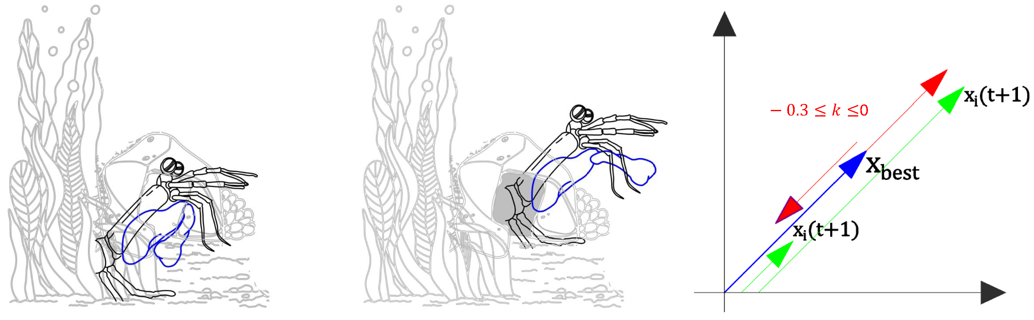
Figure 9.
Mantis shrimp’s attack strike.
Figure 9.
Mantis shrimp’s attack strike.
Figure 10.
Burrow, defense, or shelter strategy.
Figure 10.
Burrow, defense, or shelter strategy.
Figure 11.
Convergence performances of unimodal function F3 and multimodal function F14.
Figure 11.
Convergence performances of unimodal function F3 and multimodal function F14.
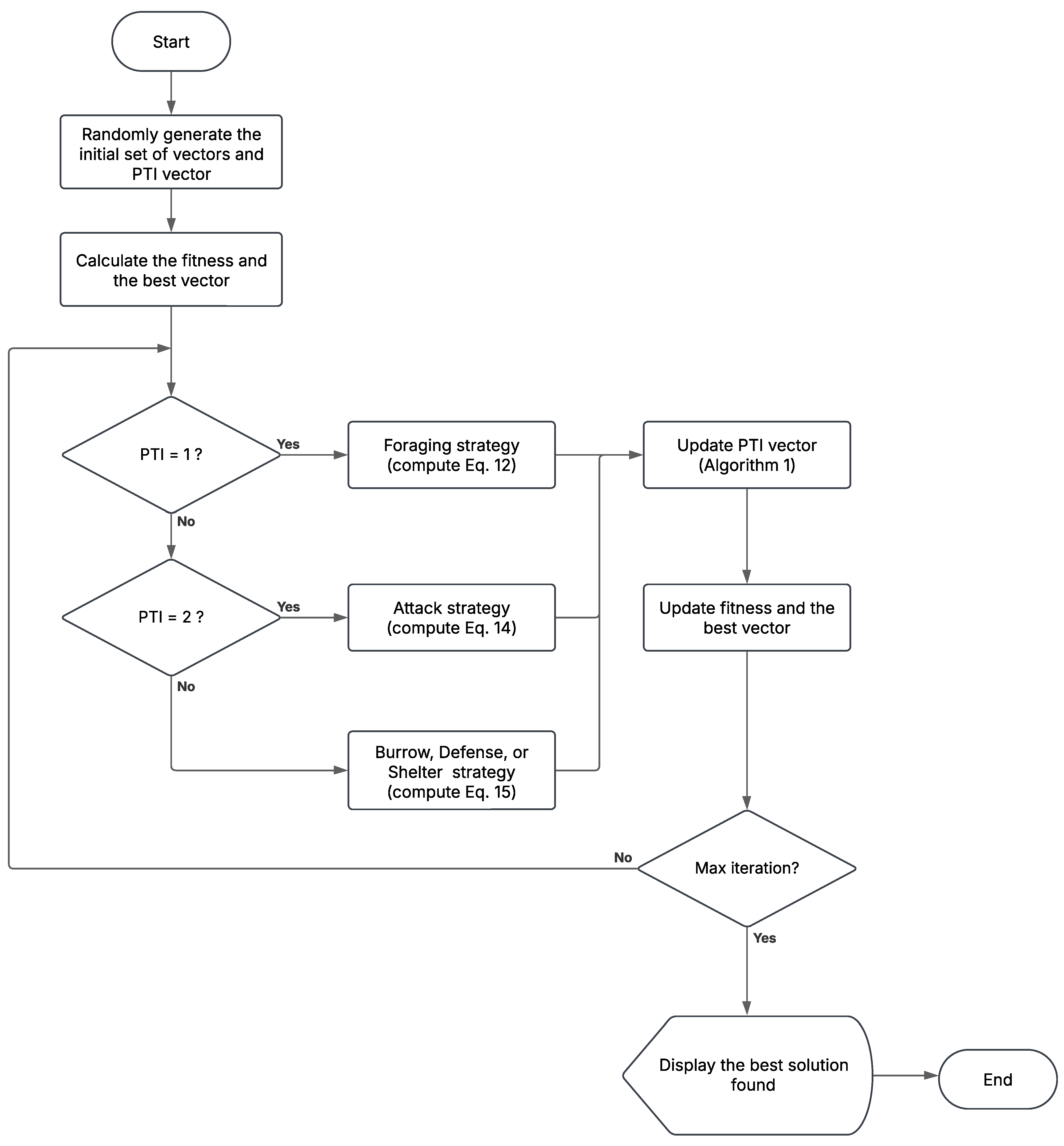
Figure 12.
MShOA flowchart.
Figure 12.
MShOA flowchart.
Figure 13.
Convergence curves of 10 unimodal functions.
Figure 13.
Convergence curves of 10 unimodal functions.
Figure 14.
Convergence curves of 10 multimodal functions.
Figure 14.
Convergence curves of 10 multimodal functions.
Figure 15.
Convergence graph of the process synthesis problem.
Figure 15.
Convergence graph of the process synthesis problem.
Figure 16.
Convergence graph of the process synthesis and design problem.
Figure 16.
Convergence graph of the process synthesis and design problem.
Figure 17.
Convergence graph of the process flow sheeting problem.
Figure 17.
Convergence graph of the process flow sheeting problem.
Figure 18.
Convergence graph of the weight minimization of a speed reducer.
Figure 18.
Convergence graph of the weight minimization of a speed reducer.
Figure 19.
Convergence graph of the tension/compression spring design (case 1).
Figure 19.
Convergence graph of the tension/compression spring design (case 1).
Figure 20.
Convergence graph of the welded beam design.
Figure 20.
Convergence graph of the welded beam design.
Figure 21.
Convergence graph of the multiple disk clutch brake design problem.
Figure 21.
Convergence graph of the multiple disk clutch brake design problem.
Figure 22.
Convergence graph of the planetary gear train design optimization problem.
Figure 22.
Convergence graph of the planetary gear train design optimization problem.
Figure 23.
Convergence graph of the tension/compression spring design (case 2).
Figure 23.
Convergence graph of the tension/compression spring design (case 2).
Figure 24.
Convergence graph of Himmelblau’s function.
Figure 24.
Convergence graph of Himmelblau’s function.
Figure 25.
IEEE 30-bus system.
Figure 25.
IEEE 30-bus system.
Figure 26.
Case 1: minimization of fuel cost.
Figure 26.
Case 1: minimization of fuel cost.
Figure 27.
Case 2: minimization of active power transmission losses.
Figure 27.
Case 2: minimization of active power transmission losses.
Figure 28.
Case 3: minimization of reactive power transmission losses.
Figure 28.
Case 3: minimization of reactive power transmission losses.
Table 1.
Behavioral strategies of the mantis shrimp based on detected polarized light.
Table 1.
Behavioral strategies of the mantis shrimp based on detected polarized light.
| Type of Detected Light by Mantis Shrimp | Action to Take |
|---|
| Vertical linearly polarized light | Foraging |
| Horizontal linearly polarized light | Attack |
| Circularly polarized light | Burrow, defense, or shelter |
Table 2.
Comparative performances of MShOA with to on benchmark functions.
Table 2.
Comparative performances of MShOA with to on benchmark functions.
| K Value | | | K = 0.1 | | | K = 0.2 | |
|---|
| F | | Best | Ave | Std | Best | Ave | Std |
| F1 | 0 | 0 | 0 | 0 | 0 | 0 | 0 |
| F2 | 0 | 0 | 0 | 0 | 0 | 0 | 0 |
| F3 | 0 | 0 | | 0 | 0 | | 0 |
| F4 | 0 | 0 | | 0 | 0 | | 0 |
| F5 | 0 | 0 | | 0 | 0 | | 0 |
| F6 | 0 | 0 | 0 | 0 | 0 | 0 | 0 |
| F7 | 0 | 0 | 0 | 0 | 0 | 0 | 0 |
| F8 | 0 | 0 | 0 | 0 | 0 | 0 | 0 |
| F9 | −1 | | | 0 | | | 0 |
| F10 | 0 | 0 | 0 | 0 | 0 | 0 | 0 |
| F11 | 0 | | | 0 | | | 0 |
| F12 | −4.59 | | | | | | |
| F13 | | | | | | | |
| F14 | 0 | | | | | | |
| F15 | 0 | 0 | 0 | 0 | 0 | 0 | 0 |
| F16 | 0 | | | | | | |
| F17 | 0 | 0 | 0 | 0 | 0 | 0 | 0 |
| F18 | 0 | | | | | | |
| F19 | 0 | | | | | | |
| F20 | −1 | | | 0 | | | 0 |
Table 3.
Continuation of comparative performances of MShOA with to on benchmark functions.
Table 3.
Continuation of comparative performances of MShOA with to on benchmark functions.
| K Value | | | K = 0.3 | | | K = 0.4 | |
|---|
| F | | Best | Ave | Std | Best | Ave | Std |
| F1 | 0 | 0 | 0 | 0 | 0 | 0 | 0 |
| F2 | 0 | 0 | 0 | 0 | 0 | 0 | 0 |
| F3 | 0 | 0 | | 0 | 0 | | 0 |
| F4 | 0 | 0 | | 0 | 0 | | 0 |
| F5 | 0 | 0 | | 0 | 0 | | 0 |
| F6 | 0 | 0 | 0 | 0 | 0 | 0 | 0 |
| F7 | 0 | 0 | 0 | 0 | 0 | 0 | 0 |
| F8 | 0 | 0 | 0 | 0 | 0 | 0 | 0 |
| F9 | −1 | | | 0 | | | 0 |
| F10 | 0 | 0 | 0 | 0 | 0 | 0 | 0 |
| F11 | 0 | | | 0 | | | 0 |
| F12 | −4.59 | | | | | | |
| F13 | | | | | | | |
| F14 | 0 | | | | | | |
| F15 | 0 | 0 | 0 | 0 | 0 | 0 | 0 |
| F16 | 0 | | | | | | |
| F17 | 0 | 0 | 0 | 0 | 0 | 0 | 0 |
| F18 | 0 | | | | | | |
| F19 | 0 | | | | | | |
| F20 | −1 | | | 0 | | | 0 |
Table 4.
Continuation of comparative performances of MShOA with to on benchmark functions.
Table 4.
Continuation of comparative performances of MShOA with to on benchmark functions.
| K Value | | | K = 0.5 | | | K = 0.6 | |
|---|
| F | | Best | Ave | Std | Best | Ave | Std |
| F1 | 0 | 0 | 0 | 0 | 0 | 0 | 0 |
| F2 | 0 | 0 | 0 | 0 | 0 | 0 | 0 |
| F3 | 0 | 0 | | 0 | 0 | | 0 |
| F4 | 0 | 0 | | 0 | 0 | | 0 |
| F5 | 0 | 0 | | 0 | 0 | | 0 |
| F6 | 0 | 0 | 0 | 0 | 0 | 0 | 0 |
| F7 | 0 | 0 | 0 | 0 | 0 | 0 | 0 |
| F8 | 0 | 0 | 0 | 0 | 0 | 0 | 0 |
| F9 | −1 | | | 0 | | | 0 |
| F10 | 0 | 0 | 0 | 0 | 0 | 0 | 0 |
| F11 | 0 | | | 0 | | | 0 |
| F12 | −4.59 | | | | | | |
| F13 | | | | | | | |
| F14 | 0 | | | | | | |
| F15 | 0 | 0 | 0 | 0 | 0 | 0 | 0 |
| F16 | 0 | | | | | | |
| F17 | 0 | 0 | 0 | 0 | 0 | 0 | 0 |
| F18 | 0 | | | | | | |
| F19 | 0 | | | | | | |
| F20 | −1 | | | 0 | | | 0 |
Table 5.
Continuation of comparative performances of MShOA with to on benchmark functions.
Table 5.
Continuation of comparative performances of MShOA with to on benchmark functions.
| K Value | | | K = 0.7 | | | K = 0.8 | |
|---|
| F | | Best | Ave | Std | Best | Ave | Std |
| F1 | 0 | 0 | 0 | 0 | 0 | 0 | 0 |
| F2 | 0 | 0 | 0 | 0 | 0 | 0 | 0 |
| F3 | 0 | 0 | | 0 | 0 | | 0 |
| F4 | 0 | 0 | | 0 | 0 | | 0 |
| F5 | 0 | 0 | | 0 | 0 | | 0 |
| F6 | 0 | 0 | 0 | 0 | 0 | 0 | 0 |
| F7 | 0 | 0 | 0 | 0 | 0 | 0 | 0 |
| F8 | 0 | 0 | 0 | 0 | 0 | 0 | 0 |
| F9 | −1 | | | 0 | | | 0 |
| F10 | 0 | 0 | 0 | 0 | 0 | 0 | 0 |
| F11 | 0 | | | 0 | | | 0 |
| F12 | −4.59 | | | | | | |
| F13 | | | | | | | |
| F14 | 0 | | | | | | |
| F15 | 0 | 0 | 0 | 0 | 0 | 0 | 0 |
| F16 | 0 | | | | | | |
| F17 | 0 | 0 | 0 | 0 | 0 | 0 | 0 |
| F18 | 0 | | | | | | |
| F19 | 0 | | | | | | |
| F20 | −1 | | | 0 | | | 0 |
Table 6.
Continuation of comparative performances of MShOA with to on benchmark functions.
Table 6.
Continuation of comparative performances of MShOA with to on benchmark functions.
| K Value | | | K = 0.9 | |
|---|
| F | | Best | Ave | Std |
| F1 | 0 | 0 | 0 | 0 |
| F2 | 0 | 0 | 0 | 0 |
| F3 | 0 | 0 | | 0 |
| F4 | 0 | 0 | | 0 |
| F5 | 0 | 0 | | 0 |
| F6 | 0 | 0 | 0 | 0 |
| F7 | 0 | 0 | 0 | 0 |
| F8 | 0 | 0 | 0 | 0 |
| F9 | −1 | | | 0 |
| F10 | 0 | 0 | 0 | 0 |
| F11 | 0 | | | 0 |
| F12 | −4.59 | | | |
| F13 | | | | |
| F14 | 0 | | | |
| F15 | 0 | 0 | 0 | 0 |
| F16 | 0 | | | |
| F17 | 0 | 0 | 0 | 0 |
| F18 | 0 | | | |
| F19 | 0 | | | |
| F20 | − 1 | | | 0 |
Table 7.
Statistical analysis of the Wilcoxon signed-rank test that compared different values of the parameter k in MShOA for 10 unimodal and 10 multimodal functions using a 5% significance level.
Table 7.
Statistical analysis of the Wilcoxon signed-rank test that compared different values of the parameter k in MShOA for 10 unimodal and 10 multimodal functions using a 5% significance level.
| k = 0.3 vs. k = 0.1 | | k = 0.3 vs. k = 0.2 | | k = 0.3 vs. k = 0.4 | |
|---|
| (+/=/−) | p-Value | (+/=/−) | p-Value | (+/=/−) | p-Value |
| (5/13/2) | | (3/13/4) | | (4/13/3) | |
| k = 0.3 vs. k = 0.5 | | k = 0.3 vs. k = 0.6 | | k = 0.3 vs. k = 0.7 | |
| (+/=/−) | p-Value | (+/=/−) | p-Value | (+/=/−) | p-Value |
| (4/13/3) | | (5/13/2) | | (5/13/2) | |
| k = 0.3 vs. k = 0.8 | | k = 0.3 vs. k = 0.9 | | | |
| (+/=/−) | p-Value | (+/=/−) | p-Value | | |
| (4/13/3) | | (3/13/4) | | | |
Table 8.
Description of the MShA algorithm’s computational complexity.
Table 8.
Description of the MShA algorithm’s computational complexity.
| Instruction | Big-O Notation | Observation |
|---|
| Initial population | | No loop is related. |
| Polarization Type Indicator | | No loop is related. |
| Strategy 1: foraging (Equation (12)) | | Consists of a sequence of constant operations. It does not depend on the input size or iterable data structures, and the loop is related to . |
| Strategy 2: attack (Equation (14)) | | Consists of a sequence of constant operations. It does not depend on the input size or iterable data structures, and the loop is related to . |
| Strategy 3: burrow, defense, or shelter (Equation (15)) | | Consists of a sequence of constant operations. It does not depend on the input size or iterable data structures, and the loop is related to . |
| Update Polarization Type Indicator (PTI) by Algorithm 1 | | Algorithm 1 consists of a sequence of constant operations. It does not depend on the input size or iterable data structures, and the loop is related
to . |
| Update population | | The loop is related to . |
| Update fitness | | The loop is related to . |
Table 9.
Initial parameters for each algorithm.
Table 9.
Initial parameters for each algorithm.
| Algorithm | Parameters | Value |
|---|
| For all algorithms | Population size for all problems | 30 |
| | Maximum iterations for testbench functions and real-world problems | 200 |
| | Number of repetition for testbench functions | 30 |
| MShOA | Does not use additional parameters | - |
| ALO | I ratio | 10 |
| | w | 2.0–0.6 |
| AOA | | 5.0 |
| | | 0.5 |
| BWO | | [0.1, 0.05] |
| DO | | [0, 1] |
| | k | [0, 1] |
| EMA | r | [0, 0.2] |
| | | [0, 1] |
| GWO | | 2.0–0.0 |
| LCA | f | 1 |
| MAO | | 0.5 |
| | | 0.1 |
| | k | 3 |
| | | 0.5 |
| MPA | P | 0.5 |
| | | 0.2 |
| SSA | v | 0.0 |
| SSOA | w | 0.7 |
| | | 2.0 |
| | | 2.0 |
| | k | 0.5 |
| TSA | | 1 |
| | | 4 |
| WOA | | 2.0–0.0 |
| | b | 2.0 |
| CFOA | Does not use additional parameters | − |
Table 10.
Comparative performances of MShOA and 14 algorithms on benchmark functions.
Table 10.
Comparative performances of MShOA and 14 algorithms on benchmark functions.
| Algorithms | | | MShOA | | | GWO | |
|---|
| F | | Best | Ave | Std | Best | Ave | Std |
| F1 | 0 | 0 | 0 | 0 | | | |
| F2 | 0 | 0 | 0 | 0 | | | |
| F3 | 0 | 0 | | 0 | | | |
| F4 | 0 | 0 | | 0 | | | |
| F5 | 0 | 0 | | 0 | | | |
| F6 | 0 | 0 | 0 | 0 | | | |
| F7 | 0 | 0 | 0 | 0 | | | |
| F8 | 0 | 0 | 0 | 0 | | | |
| F9 | −1 | −1.00 | −1.00 | 0 | | | |
| F10 | 0 | 0 | 0 | 0 | | | |
| F11 | 0 | | | 0 | | | |
| F12 | −4.59 | −4.59 | | | −4.59 | −4.59 | |
| F13 | | | | | | | |
| F14 | 0 | | | | | | |
| F15 | 0 | 0 | 0 | 0 | | | |
| F16 | 0 | | | | | | |
| F17 | 0 | 0 | 0 | 0 | | | |
| F18 | 0 | | | | | | |
| F19 | 0 | | | | | | |
| F20 | −1 | −1.00 | −1.00 | 0 | | | |
Table 11.
Continuation of comparative performances of MShOA and 14 algorithms on benchmark functions.
Table 11.
Continuation of comparative performances of MShOA and 14 algorithms on benchmark functions.
| Algorithms | | | BWO | | | DO | |
|---|
| F | | Best | Ave | Std | Best | Ave | Std |
| F1 | 0 | | | | | | |
| F2 | 0 | 0 | 0 | 0 | | | |
| F3 | 0 | | | | | | |
| F4 | 0 | | | | | | |
| F5 | 0 | | | | | | |
| F6 | 0 | 0 | 0 | 0 | | | |
| F7 | 0 | | | | | | |
| F8 | 0 | | | | | | |
| F9 | −1 | −1.00 | −1.00 | 0 | | | |
| F10 | 0 | | | | | | |
| F11 | 0 | | | 0 | | | |
| F12 | −4.59 | −4.59 | | | −4.59 | −4.59 | |
| F13 | | | | | | | |
| F14 | 0 | | | | | | |
| F15 | 0 | 0 | 0 | 0 | | | |
| F16 | 0 | | | | | | |
| F17 | 0 | | | | | | |
| F18 | 0 | | | | | | |
| F19 | 0 | | | | | | |
| F20 | −1 | −1.00 | −1.00 | 0 | | | |
Table 12.
Continuation of comparative performances of MShOA and 14 algorithms on benchmark functions.
Table 12.
Continuation of comparative performances of MShOA and 14 algorithms on benchmark functions.
| Algorithms | | | WOA | | | MPA | |
|---|
| F | | Best | Ave | Std | Best | Ave | Std |
| F1 | 0 | | | | | | |
| F2 | 0 | 0 | | | | | |
| F3 | 0 | | | | | | |
| F4 | 0 | | | | | | |
| F5 | 0 | | | | | | |
| F6 | 0 | | | | | | |
| F7 | 0 | | | | | | |
| F8 | 0 | | | | | | |
| F9 | −1 | −1.00 | −1.00 | | | | |
| F10 | 0 | | | | | | |
| F11 | 0 | | | | | | |
| F12 | −4.59 | −4.59 | −4.59 | | −4.59 | −4.59 | |
| F13 | | | | | | | |
| F14 | 0 | | | | | | |
| F15 | 0 | 0 | | | | | |
| F16 | 0 | | | | | | |
| F17 | 0 | | | | | | |
| F18 | 0 | | | | | | |
| F19 | 0 | | | | | | |
| F20 | −1 | −1.00 | | | | | |
Table 13.
Continuation of comparative performances of MShOA and 14 algorithms on benchmark functions.
Table 13.
Continuation of comparative performances of MShOA and 14 algorithms on benchmark functions.
| Algorithms | | | LCA | | | SSA | |
|---|
| F | | Best | Ave | Std | Best | Ave | Std |
| F1 | 0 | | | | | | |
| F2 | 0 | | | | | | |
| F3 | 0 | | | | | | |
| F4 | 0 | | | | | | |
| F5 | 0 | | | | | | |
| F6 | 0 | | | | | | |
| F7 | 0 | | | | | | |
| F8 | 0 | | | | | | |
| F9 | −1 | −1.00 | | | | | |
| F10 | 0 | | | | | | |
| F11 | 0 | | | | | | |
| F12 | −4.59 | | | | −4.59 | −4.59 | |
| F13 | | | | | | | |
| F14 | 0 | | | | | | |
| F15 | 0 | | | | | | |
| F16 | 0 | | | | | | |
| F17 | 0 | | | | | | |
| F18 | 0 | | | | | | |
| F19 | 0 | | | | | | |
| F20 | −1 | | | | | | |
Table 14.
Continuation of comparative performances of MShOA and 14 algorithms on benchmark functions.
Table 14.
Continuation of comparative performances of MShOA and 14 algorithms on benchmark functions.
| Algorithms | | | EMA | | | ALO | |
|---|
| F | | Best | Ave | Std | Best | Ave | Std |
| F1 | 0 | | | | | | |
| F2 | 0 | | | | | | |
| F3 | 0 | | | | | | |
| F4 | 0 | | | | | | |
| F5 | 0 | | | | | | |
| F6 | 0 | | | | | | |
| F7 | 0 | | | | | | |
| F8 | 0 | | | | | | |
| F9 | −1 | | | | −1.00 | | |
| F10 | 0 | | | | | | |
| F11 | 0 | | | | | | |
| F12 | −4.59 | −4.59 | | | −4.59 | −4.59 | |
| F13 | | | | | | | |
| F14 | 0 | | | | | | |
| F15 | 0 | | | | | | |
| F16 | 0 | | | | | | |
| F17 | 0 | | | | | | |
| F18 | 0 | | | | | | |
| F19 | 0 | | | | 0 | | |
| F20 | −1 | | | | | | |
Table 15.
Continuation of comparative performances of MShOA and 14 algorithms on benchmark functions.
Table 15.
Continuation of comparative performances of MShOA and 14 algorithms on benchmark functions.
| Algorithms | | | MAO | | | AOA | |
|---|
| F | | Best | Ave | Std | Best | Ave | Std |
| F1 | 0 | | | | | | |
| F2 | 0 | | | | | | |
| F3 | 0 | | | | | | |
| F4 | 0 | | | | | | |
| F5 | 0 | | | | | | |
| F6 | 0 | | | | 0 | 0 | 0 |
| F7 | 0 | | | | 0 | 0 | 0 |
| F8 | 0 | | | | 0 | | 0 |
| F9 | −1 | | | | −1.00 | | |
| F10 | 0 | | | | | | |
| F11 | 0 | | | | | | 0 |
| F12 | −4.59 | −4.59 | | | −4.59 | −4.59 | |
| F13 | | | | | | | |
| F14 | 0 | | | | | | |
| F15 | 0 | | | | 0 | 0 | 0 |
| F16 | 0 | | | | | | |
| F17 | 0 | | | | | | |
| F18 | 0 | | | | 0 | 0 | 0 |
| F19 | 0 | | | | | | |
| F20 | −1 | | | | | | |
Table 16.
Continuation of comparative performances of MShOA and 14 algorithms on benchmark functions.
Table 16.
Continuation of comparative performances of MShOA and 14 algorithms on benchmark functions.
| Algorithms | | | SSOA | | | TSA | |
|---|
| F | | Best | Ave | Std | Best | Ave | Std |
| F1 | 0 | | | | | | |
| F2 | 0 | 0 | 0 | 0 | 0 | | |
| F3 | 0 | | | | | | |
| F4 | 0 | | | | | | |
| F5 | 0 | | | | | | |
| F6 | 0 | 0 | 0 | 0 | 0 | 0 | 0 |
| F7 | 0 | | | | | | |
| F8 | 0 | | | | | | |
| F9 | −1 | | | | | | |
| F10 | 0 | | | | | | |
| F11 | 0 | | | 0 | | | |
| F12 | −4.59 | −4.59 | | | −4.59 | | |
| F13 | | | | | | | |
| F14 | 0 | | | | | | |
| F15 | 0 | 0 | 0 | 0 | 0 | | |
| F16 | 0 | | | | | | |
| F17 | 0 | | | | | | |
| F18 | 0 | | | | | | |
| F19 | 0 | | | | | | |
| F20 | −1 | | | | | | |
Table 17.
Continuation of comparative performances of MShOA and 14 algorithms on benchmark functions.
Table 17.
Continuation of comparative performances of MShOA and 14 algorithms on benchmark functions.
| Algorithms | | | CFOA | |
|---|
| F | | Best | Ave | Std |
| F1 | 0 | | | |
| F2 | 0 | | | |
| F3 | 0 | | | |
| F4 | 0 | | | |
| F5 | 0 | | | |
| F6 | 0 | | | |
| F7 | 0 | | | |
| F8 | 0 | | | |
| F9 | −1 | | | |
| F10 | 0 | | | |
| F11 | 0 | | | |
| F12 | −4.59 | | | |
| F13 | | | | |
| F14 | 0 | | | |
| F15 | 0 | | | |
| F16 | 0 | | | |
| F17 | 0 | | | |
| F18 | 0 | | | |
| F19 | 0 | | | |
| F20 | −1 | | | |
Table 18.
Statistical analysis of the Wilcoxon signed-rank test comparing MShOA with other algorithms for 10 unimodal functions using a 5% significance level.
Table 18.
Statistical analysis of the Wilcoxon signed-rank test comparing MShOA with other algorithms for 10 unimodal functions using a 5% significance level.
| MShOA–GWO | | MShOA–BWO | | MShOA–DO | |
|---|
| (+/=/−) | p-Value | (+/=/−) | p-Value | (+/=/−) | p-Value |
| (10/0/0) | | (7/3/0) | | (10/0/0) | |
| MShOA–WOA | | MShOA–MPA | | MShOA–LCA | |
| (+/=/−) | p-Value | (+/=/−) | p-Value | (+/=/−) | p-Value |
| (9/1/0) | | (10/0/0) | | (10/0/0) | |
| MShOA–SSA | | MShOA–EMA | | MShOA–ALO | |
| (+/=/−) | p-Value | (+/=/−) | p-Value | (+/=/−) | p-Value |
| (10/0/0) | | (10/0/0) | | (10/0/0) | |
| MShOA–MAO | | MShOA–AOA | | MShOA–SSOA | |
| (+/=/−) | p-Value | (+/=/−) | p-Value | (+/=/−) | p-Value |
| (10/0/0) | | (8/2/0) | | (8/2/0) | |
| | | MShOA–TSA | | MShOA–CFOA | |
| | | (+/=/−) | p-Value | (+/=/−) | p-Value |
| | | (9/1/0) | | (10/0/0) | |
Table 19.
Performance comparison on 10 unimodal functions by Friedman test.
Table 19.
Performance comparison on 10 unimodal functions by Friedman test.
| Algorithm | MShOA | GWO | BWO | DO | WOA |
|---|
| Mean of ranks | | | | | |
| Global ranking | | 8 | | 10 | 7 |
| Algorithm | MPA | LCA | SSA | EMA | ALO |
| Mean of ranks | | | | | |
| Global ranking | 6 | 9 | 12 | 11 | 13 |
| Algorithm | MAO | AOA | SSOA | TSA | CFOA |
| Mean of ranks | | | | | |
| Global ranking | 14 | 5 | | | 15 |
Table 20.
Statistical analysis of the Wilcoxon signed-rank test comparing MShOA with other algorithms for 10 multimodal functions using a 5% significance level.
Table 20.
Statistical analysis of the Wilcoxon signed-rank test comparing MShOA with other algorithms for 10 multimodal functions using a 5% significance level.
| MShOA–GWO | | MShOA–BWO | | MShOA–DO | |
|---|
| (+/=/−) | p-Value | (+/=/−) | p-Value | (+/=/−) | p-Value |
| (7/0/3) | | (3/4/3) | | (7/0/3) | |
| MShOA–WOA | | MShOA–MPA | | MShOA–LCA | |
| (+/=/−) | p-Value | (+/=/−) | p-Value | (+/=/−) | p-Value |
| (7/0/3) | | (7/0/3) | | (7/0/3) | |
| MShOA–SSA | | MShOA–EMA | | MShOA–ALO | |
| (+/=/−) | p-Value | (+/=/−) | p-Value | (+/=/−) | p-Value |
| (8/0/2) | | (8/0/2) | | (8/0/2) | |
| MShOA–MAO | | MShOA–AOA | | MShOA–SSOA | |
| (+/=/−) | p-Value | (+/=/−) | p-Value | (+/=/−) | p-Value |
| (8/0/2) | | (3/3/4) | | (4/3/3) | |
| | | MShOA–TSA | | MShOA–CFOA | |
| | | (+/=/−) | p-Value | (+/=/−) | p-Value |
| | | (7/0/3) | | (8/0/2) | |
Table 21.
Performance comparison on 10 multimodal functions by Friedman test.
Table 21.
Performance comparison on 10 multimodal functions by Friedman test.
| Algorithm | MShOA | GWO | BWO | DO | WOA |
|---|
| Mean of ranks | | | | | |
| Global ranking | | 8 | | 9 | 6 |
| Algorithm | MPA | LCA | SSA | EMA | ALO |
| Mean of ranks | | | | | |
| Global ranking | | 7 | 13 | 11 | 12 |
| Algorithm | MAO | AOA | SSOA | TSA | CFOA |
| Mean of ranks | | | | | |
| Global ranking | 14 | | 5 | 10 | 15 |
Table 22.
Statistical analysis of the Wilcoxon signed-rank test comparing MShOA with other algorithms for 20 functions using a 5% significance level.
Table 22.
Statistical analysis of the Wilcoxon signed-rank test comparing MShOA with other algorithms for 20 functions using a 5% significance level.
| MShOA–GWO | | MShOA–BWO | | MShOA–DO | |
|---|
| (+/=/−) | p-Value | (+/=/−) | p-Value | (+/=/−) | p-Value |
| (17/0/3) | | (10/7/3) | | (17/0/3) | |
| MShOA–WOA | | MShOA–MPA | | MShOA–LCA | |
| (+/=/−) | p-Value | (+/=/−) | p-Value | (+/=/−) | p-Value |
| (16/1/3) | | (17/0/3) | | (17/0/3) | |
| MShOA–SSA | | MShOA–EMA | | MShOA–ALO | |
| (+/=/−) | p-Value | (+/=/−) | p-Value | (+/=/−) | p-Value |
| (18/0/2) | | (18/0/2) | | (18/0/2) | |
| MShOA–MAO | | MShOA–AOA | | MShOA–SSOA | |
| (+/=/−) | p-Value | (+/=/−) | p-Value | (+/=/−) | p-Value |
| (18/0/2) | | (11/5/4) | | (12/5/3) | |
| | | MShOA–TSA | | MShOA–TSA | |
| | | (+/=/−) | p-Value | (+/=/−) | p-Value |
| | | (16/1/3) | | (18/0/2) | |
Table 23.
Performance comparison of algorithms on 20 unimodal and multimodal functions by Friedman test.
Table 23.
Performance comparison of algorithms on 20 unimodal and multimodal functions by Friedman test.
| Algorithm | MShOA | GWO | BWO | DO | WOA |
|---|
| Mean of ranks | | | | | |
| Global ranking | | 8 | | 10 | 6 |
| Algorithm | MPA | LCA | SSA | EMA | ALO |
| Mean of ranks | | | | | |
| Global ranking | 5 | 9 | 12 | 11 | 13 |
| Algorithm | MAO | AOA | SSOA | TSA | CFOA |
| Mean of ranks | | | | | |
| Global ranking | 14 | | | 7 | 15 |
Table 24.
Real-world optimization problems from the CEC2020 benchmark, where D is the problem dimension, g is the number of inequality constraints, h is the number of equality constraints, and f() is the best-known feasible objective function value.
Table 24.
Real-world optimization problems from the CEC2020 benchmark, where D is the problem dimension, g is the number of inequality constraints, h is the number of equality constraints, and f() is the best-known feasible objective function value.
| Prob | Name | D | g | h | f() |
|---|
| CEC20-RC08 | Process synthesis problem | 2 | 2 | 0 | |
| CEC20-RC09 | Process synthesis and design problem | 3 | 1 | 1 | |
| CEC20-RC10 | Process flow sheeting problem | 3 | 3 | 0 | |
| CEC20-RC15 | Weight minimization of a speed reducer | 7 | 11 | 0 | |
| CEC20-RC17 | Tension/compression spring design (case 1) | 3 | 3 | 0 | |
| CEC20-RC19 | Welded beam design | 4 | 5 | 0 | |
| CEC20-RC21 | Multiple disk clutch brake design problem | 5 | 8 | 0 | |
| CEC20-RC22 | Planetary gear train design optimization problem | 9 | 10 | 1 | |
| CEC20-RC30 | Tension/compression spring design (case 2) | 3 | 8 | 0 | |
| CEC20-RC32 | Himmelblau’s function | 5 | 6 | 0 | |
Table 25.
Results of the process synthesis problem.
Table 25.
Results of the process synthesis problem.
| Algorithms | | | |
|---|
| BWO | | | |
| MShOA | | | |
| SSOA | 0 | | * |
| AOA | | | * |
Table 26.
Comparison results of the process synthesis and design problem.
Table 26.
Comparison results of the process synthesis and design problem.
| Algorithms | | | | |
|---|
| BWO | | | |
*
|
| MShOA | | | | |
| SSOA | | | |
*
|
| AOA | | | |
*
|
Table 27.
Comparison results of the process flow sheeting problem.
Table 27.
Comparison results of the process flow sheeting problem.
| Algorithms | | | | |
|---|
| BWO | | | |
*
|
| MShOA | | | | |
| SSOA | | | | |
| AOA | | | |
*
|
Table 28.
Comparison results of the weight minimization of a speed reducer.
Table 28.
Comparison results of the weight minimization of a speed reducer.
| Parameters | BWO | MShOA | SSOA | AOA |
|---|
| | | | |
| | | | |
| | | | |
| | | | |
| | | | |
| | | | |
| | | | |
| | |
*
| |
Table 29.
Comparison results of the tension/compression spring design (case 1).
Table 29.
Comparison results of the tension/compression spring design (case 1).
| Algorithms | | | | |
|---|
| BWO | | | | |
| MShOA | | | | |
| SSOA | | | |
*
|
| AOA | | | | |
Table 30.
Comparison results of the welded beam design.
Table 30.
Comparison results of the welded beam design.
| Algorithms | | | | | |
|---|
| BWO | | | | |
*
|
| MShOA | | | | | |
| SSOA | | | | |
*
|
| AOA | | | | | |
Table 31.
Comparison results of the multiple disk clutch brake design problem.
Table 31.
Comparison results of the multiple disk clutch brake design problem.
| Variables | BWO | MShOA | SSOA | AOA |
|---|
| | | | |
| | | | |
| | | | |
| | | | |
| | | | |
|
*
| |
*
|
*
|
Table 32.
Comparison results of the planetary gear train design optimization problem (transposed).
Table 32.
Comparison results of the planetary gear train design optimization problem (transposed).
| Variables | BWO | MShOA | SSOA | AOA |
|---|
| | | | |
| | | | |
| | | | |
| | | | |
| | | | |
| | | | |
| | | | |
| | | | |
| | | | |
| | |
*
|
*
|
Table 33.
Comparison results of the tension/compression spring design (case 2).
Table 33.
Comparison results of the tension/compression spring design (case 2).
| Algorithms | | | | |
|---|
| BWO | | | | |
| MShOA | | | | |
| SSOA | | | | |
| AOA | | | | |
Table 34.
Comparison results of Himmelblau’s function.
Table 34.
Comparison results of Himmelblau’s function.
| Variables | BWO | MShOA | SSOA | AOA |
|---|
| | | | |
| | | | |
| | | | |
| | | | |
| | | | |
| *
| | *
| *
|
Table 35.
Generator inequality constraints.
Table 35.
Generator inequality constraints.
| | Min | Max | Initial |
|---|
| 50 | 200 | 99.23 |
| 20 | 80 | 80 |
| 15 | 50 | 50 |
| 10 | 35 | 20 |
| 10 | 30 | 20 |
| 12 | 40 | 20 |
| 0.95 | 1.1 | 1.05 |
| 0.95 | 1.1 | 1.04 |
| 0.95 | 1.1 | 1.01 |
| 0.95 | 1.1 | 1.01 |
| 0.95 | 1.1 | 1.05 |
| 0.95 | 1.1 | 1.05 |
Table 36.
Transformer inequality constraints.
Table 36.
Transformer inequality constraints.
| | Min | Max | Initial |
|---|
| 0.9 | 1.1 | 1.078 |
| 0.9 | 1.1 | 1.069 |
| 0.9 | 1.1 | 1.032 |
| 0.9 | 1.1 | 1.068 |
Table 37.
Shunt VAR compensator inequality constraints.
Table 37.
Shunt VAR compensator inequality constraints.
| | Min | Max | Initial |
|---|
| 0 | 5 | 0 |
| 0 | 5 | 0 |
| 0 | 5 | 0 |
| 0 | 5 | 0 |
| 0 | 5 | 0 |
| 0 | 5 | 0 |
| 0 | 5 | 0 |
| 0 | 5 | 0 |
| 0 | 5 | 0 |
Table 38.
Obtained results.
Table 38.
Obtained results.
| Minimization Studies | BWO | MShOA | SSOA | AOA |
|---|
| Fuel cost | | | | |
| Active power | | | | |
| Reactive power | | | | |


