Enhancing Recognition and Categorization of Skin Lesions with Tailored Deep Convolutional Networks and Robust Data Augmentation Techniques

Abstract

This study introduces deep convolutional neural network-based methods for the detection and classification of skin lesions, enhancing system accuracy through a combination of architectures, pre-processing techniques and data augmentation. Multiple networks, including XceptionNet, DenseNet, MobileNet, NASNet Mobile, and EfficientNet, were evaluated to test deep learning’s potential in complex, multi-class classification tasks. Training these models on pre-processed datasets with optimized hyper-parameters (e.g., batch size, learning rate, and dropout) improved classification precision for early-stage skin cancers. Evaluation measures such as accuracy and loss confirmed high classification efficiency with minimal overfitting, as the validation results aligned closely with training. DenseNet-201 and MobileNet-V3 Large demonstrated strong generalization abilities, whereas EfficientNetV2-B3 and NASNet Mobile achieved the best balance between accuracy and efficiency. The application of different augmentation rates per class also enhanced the handling of imbalanced data, resulting in more accurate large-scale detection. Comprehensive pre-processing ensured balanced class representation, and EfficientNetV2 models achieved exceptional classification accuracy, attributed to their optimized architecture balancing depth, width, and resolution. These models showed high convergence rates and generalization, supporting their suitability for medical imaging tasks using transfer learning.

1. Introduction

Skin cancer manifests itself as an abnormal development of skin cells. This article focuses on epidermal skin cancer, whereas malignant growth can affect both the epidermis and the dermis. The function of the skin is to protect us from dangerous substances and injuries. 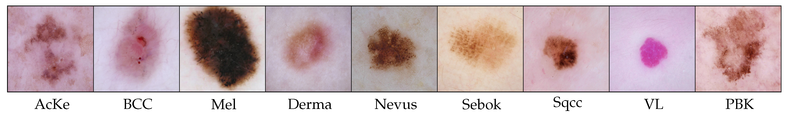Although often the exact reasons for cancer cannot be determined, it is widely known that some factors like exposure to UV radiation, a weaker immune system, and family genetics are linked to the disease [1,2,3]. The skin is protected from the effects of UV radiation by the pigment melanin’s capacity to absorb these rays. When comparing different types of lesions, particular dermoscopic characteristics are frequently considered: pre-processing, feature extraction, and image segmentation. Tumors can be classified into two main categories: malignant and noncancerous. The former includes nine basic types: dermatofibroma (Derma), melanoma (Mel), vascular lesion (VL), squamous cell carcinoma (Sqcc), actinic keratoses (Acke), benign keratosis-like lesion (BKL), and seborrheic keratosis (Sebok). Skin cancer is second in mortality behind cardiovascular disease and has become more commonplace worldwide. Clinical examinations, dermoscopic assessment, and histological methods are used during the diagnosis process [4].

According to the World Health Organization, one-third of all reported cases of cancer are skin cancer, and the prevalence rate is rising worldwide; skin cancer ranks sixth among all cancers that cause deaths in the United States. It accounts for 4% of all cancer-related deaths and six of every seven skin cancer-related deaths [5]. A medical professional must take several actions to recognize skin cancer: lesions are examined with the unaided eye during the initial phase; dermoscopy is used to investigate the structure of skin lesions in more detail; then, a biopsy is conducted, which is the process of removing a portion of the concerned skin area and sending it to a lab for microscopy investigation to conduct a more thorough analysis.

Skin cancer can be cured effectively and prevented from spreading if it is diagnosed early. Additionally, a lower death rate and less expensive medical procedures are associated with the early identification of skin cancer; see [6,7]. In addition, the manual method of examining skin cancer is laborious and may lead to human mistakes during the diagnosing process. The fine-grained lesion size and small variations in dimension, form, appearance, and color across different skin surfaces make dermoscopic images challenging to classify and detect in the early stages of cancer. Due to these complications, noise and change in intensity and similarity amongst lesions, visual approaches may result in mistakes. However, it is subjective and difficult to identify with the naked eye. The clinical diagnosis technique has a 65–80% accuracy rate in detecting melanoma. Compared to a simple subjective inspection, a more specific diagnosis can be obtained using dermoscopy images. Obtaining an enhanced view of a specific area of skin can be achieved by dermoscopy, a non-intrusive skin imaging method; see [8,9,10,11]. Between the dermoscopy-based diagnosis determination and the histological gold standard, Ascierto et al. [12] demonstrated a median consistency of 87.3%. This caused the analysis of dermoscopic pictures using various computational approaches to become a focus of study.

During the past ten years, automated medical procedures have become more common; computer-aided analysis and categorization have emerged as useful diagnostic instruments to meet these issues. Historically, several characteristics of the skin, including color, texture, form and so forth, have been employed. It takes a lot of time and is a complicated process to extract various features. With convolutional neural networks (CNNs), deep learning architectures can extract numerous features more effectively than more conventional techniques [13,14]. Figure 1 shows examples of skin cancer images considered in this research work. The literature has a variety of CNN-based designs used to identify skin cancer. All the models that are provided in this research categorize pigmented skin lesions into nine distinct malignant groups. Our goal is to characterize lesions regardless of the subclasses in which they fall [15,16,17]. These are the primary contributions of this contribution:

• We suggest a better loss function that incorporates SoftMax loss, categorical cross-entropy, and the Rectified Linear Unit (ReLU) activation function. During the training phase, it can address more effectively the issue of unbalanced multi-classification data. It may regulate the degree of difficulty in classifying samples as well as the amount of weight of negative and positive samples. Furthermore, this enhanced loss function has achieved outstanding classification performance.
• Our proposal is a Dense CNN (DCNN) architecture that improves skin cancer classification accuracy, especially for individuals in the stages of the disease.
• To solve imbalanced, mislabeled, and inadequate data samples, we present a skin cancer enhancement-based data augmentation strategy. Additionally, it increases the sample size to a larger extent and produces high-quality skin lesion images to help physicians make more precise diagnoses.
• Comparing our proposed novel skin cancer image categorization architecture to existing approaches, we achieve cutting-edge outcomes on nine types of skin lesions. The study includes the analysis of these multiple types of skin lesions by multiple neural networks.
• Compared to other transfer learning techniques including ResNet [18], AlexNet [19], VGG16, and VGG19 [20], our suggested DCNN models require a significantly shorter execution time and trainable parameters to process better output results.
• Our strategy works well and is tested against the open access ISIC dataset. The suggested model performs more accurately than the current machine learning/deep learning (ML/DL) models.
• Random values are produced following a uniform probability distribution using the Mersenne Twister method [21] with the seed initiated being based on the current time before each experiment in order to avoid repetitions. Vice versa, throughout data splitting, sampling, and augmentation procedures, a fixed random seed equal to 42 is employed to guarantee reproducibility.

This is how the remainder of the paper is designed: Section 2 pertains to a survey of the literature and related works. The methodology and processing features are explained in Section 3 and Section 4. A review of the considered convolutional neural networks is given in Section 5. The experimental results are covered in Section 6 with a brief comparison in Section 7. The conclusions are given in Section 8.

2. Related Works

Currently, there are several ML multi-type skin cancer categorization methods that have been developed, which may be broadly categorized into four groups: ensemble-based models, DCNN, transfer learning, and feature clustering. We mainly discuss the CNN and DCNNs models for the purposes of this work. A revised CNN framework was proposed by Esteva et al. [22] to speed up training. Younis et al. [23] optimized MobileNet [24] for skin cancer categorization to reduce the computational overhead, resulting in good accuracy with less computing power. However, the effectiveness of classification was damaged by other methods, such as improved optimization [25] and tailoring pre-trained methods [26]. The accuracy of a vanilla CNN that manually upsamples class probabilities was shown to be high [3]. To reduce computational cost, dimension reduction was necessary for other pre-trained CNNs such as AlexNet, MobileNet, VGG-19 and ResNet50 [27,28].

Swetha et al. [29] created the multiple classes skin tumor categorization using DCNN and transfer learning. In classifying skin lesions, the performance of several pre-trained models such as XceptionNet, ResNet50, ResNet101, ResNet152, VGG16, and VGG19 was compared. Now, 10,015 dermoscopic images representing seven different skin lesion classifications make up the HAM10000 dataset [30], which was used for that research. According to the findings, 83.69% was the category accuracy, 91.48% was the Top2 accuracy, and 96.19% was the Top3 accuracy. Sharafudeen et al. [31] created a unified multipurpose ensemble architecture to combine deep convolution neural representations with retrieved lesion features and patient metadata. To accurately identify skin cancer, the study attempted to incorporate transfer-learned picture features, both local and global texturing data, and clinical information using a proprietary generator. The architecture, which was trained and validated on different and specific datasets such as ISIC2020, BCN20000 + MSK, and HAM10000, incorporated numerous models in a weighted ensemble technique. Regarding each dataset, the model produced sensitivities of 93.17%, 87.78%, and 85.38% and specifics of 97.21%, 98%, and 98.41% respectively. Furthermore, the accuracies of the three dataset’s malignant classifications were 93.9%, 87.43%, and 88.93%, levels much higher than the usual rate of clinician diagnosis. A CNN ensemble architecture utilizing earlier trained DenseNet-121, VGG-16, ResNet50, EfficientNetB0, and XceptionNet was presented by Shorfuzzaman et al. [32]. Ensemble based on a multiscale CNN fusion was developed by Mahbod et al. [33], demonstrating consistent multi-type accuracy after being trained on resized images from the ISIC2018 dataset.

Hosny et al. [34] employed a DCNN to identify common nevus, atypical nevus, and melanoma from the PH2 skin cancer dataset. AlexNet was employed to categorize various skin malignancies from the PH2 dataset, drawing inspiration from multiple uses of DCNN architecture. Originally Imagenet’s visual recognition was handled by AlexNet, which has five convolution layers, a max pooling layer and three fully interconnected layers. There is not a pooling layer in the third or fourth convolution layer. A SoftMax layer was added in place of the last layer of the AlexNet in that work to categorize skin lesions; weights were updated using a stochastic gradient and refined via backpropagation. DenseNet-201 and StyleGAN were utilized by Zhao et al. [35] to categorize dermoscopy images from the well-balanced ISIC2019 dataset with an identification accuracy of 93.64%. Using interpretable deep learning techniques, Thomas et al. [36] suggested the multi-class classification and segmentation of skin cancer. The gray-scale images were first divided into segments, then CNN classification was performed utilizing the characteristics from the segmented images, though their suggested approach requires a lot of calculation. Using deep neural networks, Akkoca Gaziolu, and Kamaak [37] investigated how image quality affected the categorization of melanoma: they found that noisy and blurry images had an impact on how well the DL models performed in classification tasks. Generative adversarial networks (GANs) were used by Rashid et al. [38] to supplement skin lesion picture data. The GAN discriminator served as the last classifier, learning to recognize seven types of skin cancer from the ISIC2018 datasets [39]. The authors compared also the classification performance of the GAN augmentation framework with the DenseNet and ResNet architectures after fine-tuning via transfer learning [40]. The suggested approach significantly improved the balance accuracy score.

A lot of physicians have a tendency to take a camera photograph of a lesion in order to record the dermoscopic morphology of the lesion. Thankfully, most handheld dermoscopes may be equipped with adapters that allow the dermatoscope to be connected directly to the camera. Furthermore, there are dermoscopic camera lenses that are specifically designed for this purpose; they may be easier to operate than handheld devices that are connected to a camera. Finally, a lot of businesses are currently making dermoscopic lenses that are simple to attach to cellphones. The quality of these dermoscopic images is comparable to images obtained using more conventional techniques. Today, the majority of photos are taken digitally. There are several picture database applications that can make organizing and retrieving photographs easier. Lastly, a lot of the more recent whole body digital systems enable serial dermoscopy, the capture of dermoscopy, and the linking of the pictures to the diagnostic lesions [41].

The different types and sources of images can cause some challenges when it comes to detecting skin cancer [42]. The complexity of detecting skin cancer is exacerbated by the variations in human skin color appearance [43]. The following describes these difficulties as well as the most noticeable features of images of skin lesions:

• One of the biggest problems is the inefficiency of using neural networks to diagnose skin cancer; a lot of time and powerful hardware are needed before they are capable of deciphering features from images.
• Artificial Neural Networks (ANNs) require powerful GPUs to extract the features of a picture and to make a precise determination of skin cancer during the training phase of the model. However, once the model is learned, the computational load can be greatly decreased during the inference phase or normal use. This makes CNN-based systems more practical for use in the real world.
• Medical imagery typically includes certain artifacts that potentially undermine correct analysis. Inadequate contrast from adjacent tissues might occasionally present further challenges and make it more difficult to accurately analyze skin cancer. Therefore, these elements should be carefully monitored during pre-processing without affecting the important features of the data.
• Another difficulty in the identification of skin cancer is the existing bias, which alters the models’ performance to achieve a better outcome.
• Furthermore, most of the research has shown that when a lesion is less than 6 mm, scaling is crucial because it significantly lowers the diagnostic efficacy and prevents diagnosis.
• Skin cancer poses significant challenges due to the wide range of picture sizes and forms that make proper identification impossible.

3. Proposed Methodology

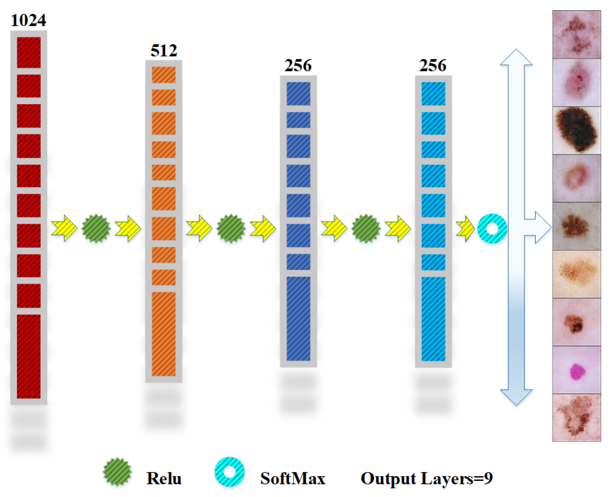
We present a deep learning architecture for skin cancer detection and classification, considering feature extraction and optimization, data augmentation, and numerous pre-processing steps for classification. We employed multiple deep learning models on the large dataset of nine types of skin cancer and then augmented the datasets to a more larger amount of data for better precision and accuracy. We employed multiple neural net approaches for better classification of multi-type skin cancer. A basic layout of this study is in Figure 2; a brief graphical description of the multiple layers and activation functions used in the structure of the CNN is in Figure 3. A short description of the CNN models is presented below.

3.1. Pooling Layers

A pre-trained model is applied first, and then a global average pooling (GAP) 2D layer is used. The pooling process determines the average value of each feature map (channel) in the preceding convolutional layer [44]. The feature map’s spatial dimensions are lowered to one value per channel. GAP is frequently used to move from convolutional layers to fully connected layers [45]. It assists in decreasing the number of network parameters and lessens the sensitivity of the model to spatial translations in the input images. Unlike Max Pooling, GAP does not require extra learnable parameters, which makes it easier to set up and less susceptible to overfitting. Let us use dimensions to represent the input features map: $P\times Q\times R$, where R is the number of channels, and P and Q are the height and width of the feature map. The mathematical expression for GAP is

$$GAP\left(y_{jkl}\right)={\displaystyle \frac{1}{P\times Q}}\sum _{j=1}^P\sum _{k=1}^Q{y}_{jkl}$$

(1)

where $y_{jkl}$ represents the value of activation at $(j,k,l)$.

To guarantee that the input is standardized for the following layer by scaling and offsetting the data from the preceding layer, we used “batch normalization” layers in between convolutional layers to provide scalability and offset factors. Neural network training can be greatly enhanced by batch normalization, which produces faster convergence, greater performance, and more consistent training patterns [3]. Following the flattening of the $3D$ feature map’s space produced during the features extracting phase, fully connected layers, also referred to as dense layers, are formed; they act as a link between the input layer and the output layer, making it easier to extract useful characteristics from the input data [46].

3.2. Activation Functions

The dense layer incorporates individual neuron weights and biases when computing the weighted sum of inputs from the preceding layer during the forward pass. The weighted sum is activated by non-linear functions like SoftMax and ReLU that increase the network’s capacity to represent intricate correlations in the data [47]. The dense layer uses optimization algorithms to align its parameters to minimize a predetermined loss function over iterative training epochs. Through this process, the network learns and adapts itself over time, eventually identifying complex patterns and representations in the data. The SoftMax and ReLU activation functions are given in Equations (2) and (3), respectively. The layer’s output is subjected to the SoftMax function to calculate the probability distribution across the classes:

$$S\left(z_j;y\right)={\displaystyle \frac{e^{x_k}}{{\sum }_k{e}^{x_k}}}.$$

(2)

$$S\left(z\right)=z^{+}=max\left(0,z\right),$$

(3)

with $S\left(z_j;y\right)$ being the probability of j, and input z and $x_k$ being the output of j.

3.3. Loss Functions

An optimization technique that is frequently used in machine learning, especially for neural network training, is the so-called Stochastic Gradient Descent (SGD). In order to minimize a loss function, a measure of the discrepancy between the expected and actual results, the SGD optimizer iteratively modifies the model’s parameters. SGD modifies the parameters according to a single training example or a small batch of examples, in contrast to traditional gradient descent, which computes gradients using the whole dataset. Because of their stochastic nature, the gradient estimates contain noise that may assist researchers avoid local minima and leads to better results. The primary benefit of SGD over batch gradient descent is its ability to converge rapidly, particularly when dealing with large datasets. The SGD algorithm minimizes the loss function $L\left(\theta \right)$ by iteratively adjusting the model’s parameters, or weights. The rule is given as follows:

$${\vartheta }_j^{\left(t+1\right)}={\vartheta }_j^{\left(t\right)}-\beta {\displaystyle \frac{𝜕L\left(\vartheta \right)}{𝜕{\vartheta }_j}}$$

(4)

where ${\vartheta }_j^{\left(t\right)}$ is the parameter value of j at iteration t, $\beta$ is the learning rate, and ${\displaystyle \frac{𝜕L\left(\vartheta \right)}{𝜕{\vartheta }_j}}$ is the loss function gradient. The gradient of the loss function with respect to that parameter is subtracted, and the result is the updated parameter. The parameters are modified iteratively to thus minimize the loss function.

3.4. Dropout Layers

Without significantly compromising the model’s capacity for learning, we used “dropout layers” to efficiently switch off certain neurons to prevent over-fitting and to reduce the overall computing complexity. The order of the layers and the quantity of dropout layers serve as the main points of differentiation. Every dense layer in the script is followed, apart from the final one, by a dropout layer with a dropout rate of 0.5. Accordingly, a dropout layer is added after the flatten layer, followed by a dense layer. For each update during training, a random fraction of the input units is set to zero, which helps keep the units from excessively co-adapting. It helps in enhancing the model’s capacity for generalization; dropout layers contribute to the regularization [48]. A key element of neural network training for multi-class classification problems is the categorical cross-entropy loss function, which penalizes the model according to the discrepancy between the true and predicted class probabilities. During training, the cross-entropy loss function was utilized. This function is very useful whenever the training datasets are non-uniform. In machine learning, multi-classification problems are primarily solved via cross-entropy [26]. A loss function called categorical cross-entropy is applied to multi-class classification assignments, in which the output variable contains more than two classes. The categorical cross-entropy loss function is defined as follows for a multi-class classification problem with C classes:

$$L_R\left(\vartheta \right)=-ln{\displaystyle \frac{e^{\left({\vartheta }_t\right)}}{{\sum }_{i=1}^C{e}^{\left({\vartheta }_i\right)}}}.$$

(5)

The positive class distribution for all C classes is represented by ${\vartheta }_t$, where i indicates the number of iterations.

4. Pre-Processing

The first need for achieving state-of-the-art performance with deep learning models is a tidy and proficient dataset. The ISIC dataset [28] used in this study was obtained from Kaggle [27] (example images in Figure 1). This dataset contains nine categories and has 2357 pictures in total. A crucial first step in improving any dataset’s quality is the pre-processing of data. Certain images in the collection have low pixel dimensions, so image creation parameters can vary. All images should be scaled to a particular size in the first step of the pre-processing. We scaled all the images in the dataset to a fixed size of $224\times 224$. We extracted a vast variety of features to aid in identifying and recognizing patterns across a multitude of datasets [49]. Furthermore, it chooses and mixes variables to extract characteristics that reduce the number of resources without erasing any raw data information [50].

Before augmentation and training, the dataset was carefully cleaned to assure data integrity and to eliminate eventual bias. This involved the elimination of indistinct, noisy, and low-resolution photos, discovered by visual inspection and filtered by analyzing unusual pixel value patterns. Identical samples were identified by perceptual hashing and file comparison methodologies. The resulting refined dataset ensured that training was established on diverse samples. We restricted the maximum number of images per class to 6500 to ensure class balance prior to augmentation.

4.1. Data Splitting

To mitigate the issue of overfitting resulting from the limited quantity of training picture datasets, the ISIC2018 dataset was divided into three mutually distinctive sets: training, validation and testing sets. The model was trained for 50 epochs; every epoch, model-augmented training photos were provided by the Image Data Generator in Keras. There are 1508, 377, and 472 photos in the train, validation, and test sets, respectively. Now, 64 is the chosen batch size for training. We used the dataset to train the different models and assess how well they detect skin cancer (

Table 1. Dataset summary.

Label	Class	Count	Train	Test	Validation
1	AcKe	130	76	33	21
2	BCC	392	253	79	60
3	Mel	454	297	75	82
4	Derma	111	66	23	22
5	Nevus	373	247	77	49
6	Sebok	80	55	12	13
7	Sqcc	197	126	41	30
8	VL	142	81	29	32
9	PBK	478	307	103	68
	Total	2357	1508	472	377

).

4.2. Data Normalization

The process of designing a database that reduces data redundancy, ensures data integrity and eliminates undesirable features such as insertion, revision, and removal anomalies is known as data normalization. Rao et al. [51] identified several prevailing normalizing strategies, including min–max, z-score, decimal scaling normalization, and resizing photos to the size of $224\times 224$ pixels, which is a standard in well-known CNN architectures. Also, bilinear interpolation is commonly used when resizing.

4.3. Data Augmentation

When compared to a class with fewer training images, the one with additional training image data will be biased to obtain decent accuracy. Model overfitting is a typical issue with ML/DL models [50], particularly with smaller datasets. When a model exhibits good performance on a specific training dataset but performs poorly on a test dataset with slightly different images, it is said to be overfitting. Before using the dataset for training, “data augmentation” is carried out to guarantee that the classes in it are well balanced and we use different approaches as rotation, flipping both horizontally and vertically, shifting (i.e., translating) both horizontally and vertically, and zooming to enhance the dataset (Figure 4).

An enormous rise in the overall number of images occurs with augmentation. As a result, there would be a smaller chance of overfitting because the training dataset grows significantly [51]. Regarding dataset augmentation and image pre-processing, DataGen is a potent deep learning tool. It works by transforming input photos in several ways, producing newly enhanced representations of the initial data. It makes it possible to apply these adjustments within predetermined limits of variance, which boosts the dataset’s resilience and diversity. To teach deep learning algorithms to perform better on real-world tasks and to generalize effectively to new data, this variety is crucial.

4.4. Hyper-Parameter Settings

Table 2. Dataset summary after augmentation and normalization.

Label	Class	Count	Train	Test	Validation
1	AcKe	6500	4225	1257	1018
2	BCC	6500	4182	1277	1041
3	Mel	6500	4159	1289	1052
4	Derma	6500	4212	1285	1003
5	Nevus	6500	4134	1306	1060
6	Sebok	6500	4119	1296	1085
7	Sqcc	6500	4164	1334	1002
8	VL	6500	4225	1257	1018
9	PBK	6500	4106	1337	1060
	Total	58,500	37,440	11,700	9360

lists the hyperparameters of the proposed model, which approximate the computational complexity of a given neural network. It should be noted that the suggested design uses SoftMax activation functions for the output layer and ReLU for the hidden layer activation as stated in Equations (2) and (3). Learning rate schedulers are essential for improving the rate of convergence and consistency of deep learning models. This study uses the ReduceLROnPlateau program as a particular approach [52]. During training, the program dynamically modifies the learning rate in response to the model’s performance on the validation set. It keeps an eye on the validation accuracy and lowers the learning rate if it detects a performance plateau, which could indicate that the model is no longer performing at its best. The two most important parameters of this scheduler are the patience factor, which indicates the factor by which the learning rate is reduced, and the patience, which establishes the quantity of epochs that are necessary before decreasing the learning rate if no enhancement is seen. To stop the learning rate from falling perpetually, a minimum learning rate is set also. This adaptive learning rate modification promotes more effective optimization and makes it easier to explore the parameter space of the model, which eventually improves performance and generalization. These parameters are slightly different for the proposed models [53].

Table 3. Hyperparameter assumptions and settings.

Model	XceptionNet	DenseNet	MobileNets
Base Model	Deep CNN
Optimizer	Stochastic Gradient Descent
Batch Size	64, 80, 100, 128
No. of Epochs	50, 100, 120, 150, 200
Learning rate	0.001
Number of Dense Layers	4	3	4
No. of Classes	9
Activation Function in Hidden layers	ReLU
Activation Function in output layer	SoftMax
Loss	Categorical Cross entropy
Minimum Learning rate	0.00001
Random_state	1
Padding	Same
Patience	3	3	3
Trainable parameters (total)	40,340,785	30,548,873	18,611,977
Non-Trainable Parameters	54,528	229,056	34,112

shows the breakdown of the hyperparameter settings that are carried out, illustrating the tabular statistics of the dense layers and multi-layer structure used for application of the CNN models on the skin cancer dataset.

Grid-based empirical evaluation impact the selection of hyperparameters, including the batch size and number of training epochs. Batch sizes of 32, 64, 96, and 128 were used in our experiments. A batch size of 64 allowed for steady improvements across mini-batches while minimizing oscillations in training loss, offering the best trade-off between convergence speed and GPU memory economy. The early flattening of training and validation accuracy trends (see Section 6) suggested that 100 epochs of training were enough to achieve convergence across all models. In order to ensure greater generalization and faster convergence, we also employed a ReduceLROnPlateau callback with a patience of 3 to lower the learning rate by a factor of 0.5 when validation accuracy stalled. Overfitting was avoided because of this adaptive approach, particularly in deeper designs like DenseNet-201 and EfficientNetV2-B3. Overall, fine-tuning to balance model correctness, computational efficiency and training stability led to the chosen design.

4.5. Performance Measures

The lesion classes prediction is the final step of the suggested DNNs paradigm and is based on the combined prediction values for each class from each model. The accuracy of a model’s class prediction is used to assess classification performance. All the widely used performance measures, namely, accuracy, precision, recall, and $F1$ score, are employed in this study to support the model’s strong performance [3,51]. These measures are outlined below. More precisely, the parameter accuracy measures the statistical soundness of the detection and classification of multi-class skin cancer. Here, $FN$ stands for false negative, $FP$ for false positive and $TP$ for true positive. Because this measure depends on both the $FP$ and $FN$, relying just on it might occasionally be deceptive when assessing a predictor’s performance. This suggests that it is possible to have two models with identical accuracy, one having high $FP$ and low $FN$, and the other having low $FP$ and high $FN$. The first model can therefore be selected above the second since it has a lower $FN$ for the delicate medical case, which may not be decided solely by the model’s accuracy scores, namely,

$$Accuracy={\displaystyle \frac{TP+TN}{TP+FP+TN+FN}}.$$

(6)

The next equations determine the statistical completeness of the final prediction and hence are used to measure two performance parameters. More precisely, the percentage of real photographs in each class that match the projected images for that class is measured by precision. Conversely, recall counts how many pictures in a certain class there are overall and what percentage of those pictures are properly identified as belonging to that class, namely,

$$Precision={\displaystyle \frac{TP}{TP+FP}},$$

(7)

$$Recall={\displaystyle \frac{TP}{TP+FN}}.$$

(8)

The combination of recall and precision can be described as the weighted mean of both. Namely, we define the $F1$ score as

$$F1=2{\displaystyle \frac{Precision\times Recall}{Precision+Recall}}={\displaystyle \frac{2TP}{2TP+FP+FN}}.$$

(9)

It is also noteworthy that the precision, recall, and $F1$ score have a range of values between zero and one. A model performs better for a certain classification job if these three values are higher.

5. Convolutional Neural Networks

CNNs are very efficient in image classification, object recognition, and various computer vision applications, owing to their capacity to learn hierarchical characteristics via deep layers. This work utilizes several CNN architectures, including multiple neural networks, to achieve precise and efficient image categorization. Hence, we have used several CNN models for examining and diagnosing different skin cancer types.

5.1. XceptionNet

The XceptionNet framework is comprised of 36 CNN layers organized into 14 phases, all adhering to the depthwise separable convolution technique. The network can be divided into three primary components. It begins with a few conventional convolution layers, followed by depthwise separable convolutions that incrementally increase the number of filters while reducing spatial dimensions via striding. This section consists of eight unique modules, each comprising depthwise separable convolutions, followed by ReLU activation and batch standardization. Residual connections are employed to ensure gradient flow consistency. The Exit Flow employs depthwise separable convolutions and subsequently applies a global average pooling layer, concluding with a dense layer utilizing SoftMax activation. This structure allows XceptionNet to effectively acquire hierarchical features, making it well suited for a range of imagery applications [54].

5.2. DenseNets

DenseNet is a CNN variant that prioritizes dense linkages among layers: each layer is interconnected with all other layers in a feed-forward configuration. The output of each layer is concatenated with the inputs of all following layers hence boosting feature reuse and minimizing the number of parameters, which increases the network’s efficiency. This section delineates the DenseNet-121, DenseNet-169, and DenseNet-201 models, which differ in depth (i.e., the number of layers). These models have gained widespread acceptance owing to their capacity to alleviate the vanishing gradient issue, facilitating the more effective training of deeper networks. Compared to conventional designs, where each layer merely connects to the layer below it, this design stands in stark contrast. The attribute maps of all previous layers are sent now into the ℓ-th layer, the output of which is defined as

$$y_{𝓁}=M_{𝓁}\left(\left[y_0,y_1,...,y_{𝓁-1}\right]\right)$$

where $M_{𝓁}$ is a composite function of processes like a batch normalization, the ReLU activation, and a convolution; $\left[y_0,y_1,...,y_{𝓁-1}\right]$ is the concatenation of the map of features created by layers 0 to $𝓁-1$; and data transfer between layers is ensured by this dense connectivity design. One crucial hyperparameter in the DenseNet is its growth rate k, which indicates the quantity of feature maps that every layer contributes: a layer that receives m feature maps as input will produce $m+k$ feature maps as output. The amount of newly acquired data that each layer adds to the network’s overall state is determined by its growth rate [19,55].

The DenseNet models (121, 169, 201) adhere to the overall design, achieving a harmonious balance between depth and computational efficiency by employing a carefully designed arrangement of layers. The network starts with an initial 7 × 7 convolution layer, followed by a 3 × 3 max pooling layer of data. It consists of four dense blocks interspersed with transition layers that reduce spatial dimensions through convolution and pooling. In each dense block, there are several layers, each taking the previous feature maps as input and applying Batch Normalization, ReLU, BatchNorm, ReLU, and 3 × 3 convolution. Transition layers consist of BatchNorm and 2 × 2 average pooling. The architecture ends with a global average pooling layer and a fully connected layer that uses SoftMax activation for tasks such as classification [56,57]. The efficient design and robust reliability of DenseNet-201 have made it a successful choice in various domains. The underlying structure, model parameters and architectural elements of DenseNet-121, DenseNet-169 and DenseNet-201 are essentially equal with the distinction being the network’s depth and the consequent ability to learn intricate characteristics.

5.3. MobileNets

MobileNet-V2 network is designed to maximize performance while working within computational constraints. The reversed residuals block is a core component of this network, setting it apart from conventional block residuals found in networks such as ResNet. The input in a conventional residual block is amplified employing convolution and then modifications are carried out. MobileNet-V2 takes a different approach by initially reducing the dimensionality, implementing depthwise separable convolution, followed by re-establishing the dimension. This method ensures that a comprehensive set of features is preserved, while also minimizing the amount of computational resources required [58]. MobileNet-V2 involves linear bottleneck layers to maintain accuracy and minimize non-linearity: an inverse residuals block alongside the linear bottleneck is represented as

$$y=x+F\left(x\right)$$

where the input is denoted as x, the transformation function F consists of depthwise separate convolutions and ReLU activations, and the output is represented as y. This representation is commonly used in the field of data science [59].

Depthwise separated convolutions play an important role in the architecture of MobileNet-V2 [60]. Transition layers are inserted between residual blocks to modify the dimensionality of the feature maps. The network ends on a global average pooling layer, including a fully linked layer that uses SoftMax activation. This approach guarantees the model’s efficacy across diverse applications while preserving efficiency [61].

MobileNet-V3 Large includes inverted residual blocks and depthwise separable convolutions and incorporates significant enhancements, such as a more efficient activation function (hard-swish) and optimizations derived from Neural Architecture Search and Squeeze-and-Excitation blocks which facilitate a method of channel-wise feature recalibration to adaptively assess the significance of various feature mappings [62]. This is accomplished by initially employing global average pooling to condense the spatial dimensions of the feature maps into a singular value for each channel. The compressed information is further processed through a compact fully connected network with ReLU activation, followed by a sigmoid function, to provide weights that emphasize the most relevant aspects. This allows MobileNet-V3 to prioritize essential elements while diminishing the impact of less significant ones, hence enhancing the model’s overall efficacy in picture classification and object identification tasks [63].

MobileNet-V3-Large possesses a greater number of layers and parameters, enhancing its accuracy. Nonetheless, it necessitates somewhat more processing resources. This model includes dropout layers to mitigate overfitting by randomly deactivating a portion of neurons during the training process. Employing a dropout rate equal to 0.4 (in contrast to the conventional 0.5 rate) somewhat diminishes the dropout impact, facilitating the retention of additional features during training while still reaping the advantages of regularization [64]. A crucial element of this model is the implementation of L2 kernel regularization in the thick layers; this imposes an adjustment on the loss function proportional to the magnitude of the model’s weights, aiding in the prevention of overly large weights and thereby diminishing overfitting. L2 regularization incorporates an additional term into the loss function as

$$L_A=L_B+\lambda \sum _{j=1}^m{\omega }_j^2.$$

where $L_A$ denotes the total loss, $L_B$ represents the preliminary loss (specifically, the categorical crossentropy), ${\omega }_j$ signifies the model’s weights, and $\lambda$ indicates the regularization parameter [65]. MobileNet-V3-Large imposes a little penalty on substantial weights by using L2 with a strength of 0.001. Implementing L2 regularization enhances the model’s generalization to novel data, hence increasing its robustness and reliability. The definitive design of MobileNet-V3-Large comprises a series of inverted residual blocks with linear bottlenecks, and Squeeze-and-Excitation blocks for feature calibration, and it concludes with global average pooling and fully linked layers for classification. The integration of sophisticated features guarantees that MobileNet-V3-Large achieves a high degree of accuracy while minimizing computing expenses, rendering it appropriate for mobile and embedded applications [66].

5.4. NASNet Mobile

In contrast to manually developed topologies, NASNet Mobile is derived from Neural Architecture Search (NAS), a method that autonomously identifies and refines network structures. NAS uses reinforcement learning to identify the optimal architecture, considering the trade-off between accuracy and processing economy. NASNet Mobile utilizes normal cells for feature extraction and reduction cells for downsampling, allowing the model to excel in diverse tasks while preserving little computational cost. This model begins by importing pre-trained weights from ImageNet, facilitating transfer learning and enabling to leverage previously acquired features without training from the ground up. Subsequent to the NASNet Mobile layers, the model employs global average pooling to condense each feature map into a single value, therefore markedly decreasing the parameter count in contrast to fully linked layers. This approach mitigates overfitting by streamlining the model while preserving critical feature information [67,68].

Dropout layers are implemented at a rate of 0.4 to enhance model regularization. L2 regularization in the dense layers limits the weights, preventing them from becoming overly big and so mitigating the risk of overfitting. The network has two completely linked layers with ReLU activation function to facilitate non-linearity, enabling the network to acquire intricate representations from the data. Dropout is implemented subsequent to each thick layer to enhance the model’s generalization capacity. The terminal output layer employs the SoftMax activation function, suitable for multi-class classification problems. It generates a probability distribution across the classes, enabling the model to forecast based on the greatest likelihood. The model is created using the Adam optimizer, selected for its effective management of extensive datasets and capacity to adjust the learning rate throughout training. The initial learning rate is established at 0.0001, and a learning rate reduction approach is implemented with the ReduceLROnPlateau callback by reducing the learning rate by a factor of 0.5 if the validation accuracy fails to increase after three epochs, facilitating a more gradual convergence during model training [69,70].

EffecientNetV2-B3, which is similar to NASNet Mobile, is a compromise between accuracy and computing economy, especially in mobile and resource-limited contexts. Both models emphasize the reduction in resource use while preserving performance, although they diverge in their design methodologies and optimization strategies. This model is initialized with ImageNet pre-trained weights and makes use of a systematic scaling methodology via its compound scaling technique, optimizing the network across many dimensions (e.g., depth, breadth, and resolution). EfficientNetV2-B3 utilizes fused convolutions, integrating standard convolutions with depthwise separable convolutions [71].

5.5. Comparative Analysis of Model Characteristics

Multiple DCNN algorithms include distinct advantages that make them appropriate based on difficulty, dataset scale, and computing constraints.

Table 4. CNN designs and their significance in skin lesion classification.

Model	Key Features	Skin Lesion Applications
Xception [72]	Depthwise separable convolutions, efficient feature reuse	Melanoma detection with fine-grained features [73]
DenseNet121/169/201 [74]	Dense connections, strong gradient flow, compact model size	High accuracy in ISIC 2018 classification [75]
MobileNetV2/V3 [63,76]	Lightweight, mobile-optimized, fast inference	Deployed in real-time diagnosis apps [77]
NASNet Mobile [78]	Auto-searched modules, good trade-off between accuracy and efficiency	Used for multi-class lesion classification [79]
EfficientNetV2-B3 [80]	Compound scaling, fast convergence, state-of-the-art accuracy	Robust in ensemble models for melanoma detection [81]

outlines the architectural characteristics and principal appropriateness criteria of each assessed model for skin lesion image categorization.

6. Results and Discussions

We give the assessment findings in this section for many CNN architectures applied to skin lesion classification tasks. To improve performance and avoid overfitting, each model is specifically optimized with regard to dropout rates, learning rate modifications and L2 regularization. The outcomes provide a thorough understanding of the model’s performance and are displayed through accuracy, loss curves, and confusion matrices. Strong generalization abilities were demonstrated by the early epochs of the models, which saw rapid convergence across models, followed by consistent, high accuracy rates with little divergence between the training and validation measures. Additional evidence of good categorization ability across lesion types is provided by the confusion matrices. The comparison as a whole shows how well these models perform in terms of obtaining high accuracy, low overfitting, and efficient lesion categorization, giving medical image analysis tasks a solid basis. Table 3 gives a summary of the important hyperparameters that are employed in several CNN models.

6.1. XceptionNet

The pre-trained ImageNet model that was utilized in this experiment is XceptionNet without the top layer to allow customization. This modification included dropout layers to reduce overfitting, fully linked layers (dense layers), and flattening the output of the final convolutional layers. The architecture’s main layers are as follows, listed in

Table 5. XceptionNet implementation details.

Layer (Type)	Output Shape	No. of Parameters
XceptionNet	(None, 2, 3, 2048)	20,861,480
Flatten (Flatten)	(None, 18,432)	0
Dropout (Dropout)	(None, 18,432)	0
Dense (Dense)	(None, 1024)	18,875,392
Dropout:1 (Dropout)	(None, 1024)	0
Dense:1 (Dense)	(None, 512)	524,800
Dropout:2 (Dropout)	(None, 512)	0
Dense:2 (Dense)	(None, 256)	131,328
Dense:3 (Dense)	(None, 9)	2313
Total parameters: 40,395,313
Trainable parameters: 40,340,785
Non-trainable parameters: 54,528

:

• Base XceptionNet: This is the model’s core with over 20.8 million parameters. Quick training convergence is made possible by the pre-trained weights on ImageNet, which make use of the features that have been learned from a variety of image categories.
• Convolutional feature maps: They are flattened in the flatten layer into a one-dimensional vector, which is then sent to fully linked layers.
• Dropout layers: To minimize overfitting, a 50% dropout rate was added to different thick layers, randomly deactivating half of the neurons on each forward run.
• Dense layers: A 1024-unit dense layer with ReLU activation captures high-level abstract information. The feature extraction procedure is further improved by adding 512-unit and 256-unit dense layers.
• Last dense layer: The 9-unit and SoftMax activation of the last dense layer match the nine classes in the classification job. A projected chance for each of the nine forms of skin cancer is represented by a unit in the output.
• The learning rate is dynamically modified using the ReduceLROnPlateau callback, which decreases the learning rate using Stochastic Gradient Descent.

The performance results for various epochs and batch sizes are displayed in

Table 6. XceptionNet parameters and performance.

XceptionNet	Accuracy	Precision	Recall	F1 Score	Kappa Score	Test Acc
Epoch: 50	0.9256	0.9261	0.9242	0.9139	0.9369	0.8948
Batch Size: 64
Perclass: 6500
Epoch: 100	0.9481	0.9425	0.9498	0.9495	0.9374	0.9193
Batch Size: 120
Perclass: 8500
Epoch: 120	0.9607	0.9567	0.9516	0.9596	0.9535	0.9216
Batch Size: 150
Perclass: 7500
Epoch: 150	0.9691	0.9591	0.9692	0.9461	0.9523	0.9328
Batch Size: 150
Perclass: 9500
Epoch: 200	0.9721	0.9639	0.9615	0.9682	0.9738	0.9317
Batch Size: 150
Perclass: 6500

. After 50 epochs, the accuracy increases to 0.9256; after 200 epochs, it reaches 0.9721. Recall and precision show a similar tendency of increasing with training time. The model’s accuracy and recall are well balanced after 200 epochs, with precision reaching 0.9639 and recall standing at 0.9615. Over time, the F1 score and Kappa score also show notable improvements. After 200 epochs, the F1 score hits 0.9682, indicating the model’s resilience to unbalanced classes. Even after taking into consideration random chance, the Kappa score of 0.9738 indicates good agreement between the expected and real labels. At 50 epochs, the test accuracy is 0.8948; at 200 epochs, it is 0.9317. This validates that there is little overfitting and that the model can generalize effectively to new data.

The training and validation trends of both accuracy and loss over 100 epochs are depicted in Figure 5. The first few epochs saw a significant decrease in both training and validation losses; in the first ten epochs, the loss values went from around 1.7 to less than 0.4. This sharp decline suggests that the model is rapidly learning accurate data classification skills. Following epoch 30, the validation loss varies from 0.15 to 0.35, whereas the training loss steadies around 0.05. This pattern indicates that although the model is generalizing successfully during the training phase, the validation accuracy stays somewhat lower, ranging from 0.92 to 0.95. The model is effective as seen by the very modest difference between the training and validation accuracies.

6.2. DenseNet-121

A useful framework for managing deep learning tasks in medical image analysis is given by the DenseNet-121 architecture. With 7.33 million parameters, 7.25 million of which are trainable, the layered structure of this model is displayed in

Table 7. DenseNet-121 implementation details.

Layer (Type)	Output Shape	No. of Parameters
Densenet-121	(None, 2, 3, 1024)	7,037,504
GAP (2D)	(None, 1024)	0
Dropout(Dropout)	(None, 1024)	0
Dense (Dense)	(None, 256)	262,400
Dropout:1(Dropout)	(None, 256)	0
Dense:1 (Dense)	(None, 128)	32,896
Dense:2 (Dense)	(None, 9)	1161
Total parameters: 7,333,961
Trainable parameters: 7,250,313
Non-trainable parameters: 83,648

. Reusing features and enhancing gradient flow across layers are made easier by DenseNet, which is well known for its dense connection. To prevent overfitting, dropout layers, several dense layers, and global average pooling are all included in the framework. The input is divided into nine different groups according to a final SoftMax layer. Using a layered technique, transfer learning is utilized, wherein the top layers are optimized for the particular job, while the convolutional backbone is pre-trained on ImageNet and frozen across the training phase.

The key parameters and measures for DenseNet-121 are listed in

Table 8. DenseNet-121 parameters and performance.

DenseNet-121	Accuracy	Precision	Recall	F1 Score	Kappa Score
Epoch: 50	0.9869	0.9869	0.9864	0.9866	0.9852
Batch Size: 32
Per class: 7500
Epoch: 50	0.9944	0.9939	0.9938	0.9938	0.9937
Batch Size: 64
Per class: 7500
Epoch: 100	0.9675	0.9712	0.9688	0.9690	0.9716
Batch Size: 64
Per class: 7500
Epoch: 150	0.9916	0.9918	0.9914	0.9916	0.9905
Batch Size: 64
Per class: 7500
Epoch: 200	0.9955	0.9951	0.9950	0.9951	0.9950
Batch Size: 96
Per class: 7500

. The accuracy and loss patterns for training and validation throughout 100 epochs are displayed in Figure 6. The validation accuracy varies but remains around 98–99%, indicating a robust generalization, whereas the training accuracy increases quickly in the first 10 epochs and stabilizes around 99%. The initial few epochs see a sharp decline in the training and validation losses, which thereafter vary at lower values. The model’s capacity to minimize efficiently classification errors and to preserve robustness throughout generalization is demonstrated by the comparatively low validation loss (below 0.2) seen over most epochs.

6.3. DenseNet-169

The complexity of DenseNet-169 can be assessed by examining

Table 9. DenseNet-169 implementation details.

Layer (Type)	Output Shape	No. of Parameters
Densenet-169 (Functional)	(None, 2, 3, 1664)	12,642,880
Global Average Pooling 2d	(None, 1664)	0
Dropout (Dropout)	(None, 1664)	0
Dense (Dense)	(None, 256)	426,240
Dropout:1 (Dropout)	(None, 256)	0
Dense:1 (Dense)	(None, 128)	32,896
Dense:2 (Dense)	(None, 9)	1161
Total parameters: 13, 103,177
Trainable parameters: 12,944,777
Non-trainable parameters: 158,400

: there are 13,103,177 parameters in the model altogether, 12,944,777 of which can be trained. This large number of parameters illustrates how deep the DenseNet architecture is, making it ideal for challenging image classification applications. In terms of skin condition classification, the DenseNet-169 model performs remarkably well, attaining virtually perfect accuracy.

The model’s performance in various training setups is shown in

Table 10. DenseNet-169 parameters and performance.

DenseNet-169	Accuracy	Precision	Recall	F1 Score	Kappa SCORE
Epoch: 50	0.9930	0.9931	0.9922	0.9926	0.9921
Batch Size: 32
Per class: 7500
Epoch: 50	0.9959	0.9957	0.9953	0.9955	0.9954
Batch Size: 64
Per class: 7500
Epoch: 100	0.9597	0.9613	0.9588	0.9709	0.9693
Batch Size: 64
Per class: 7500
Epoch: 100	0.9863	0.9865	0.9862	0.9863	0.9846
Batch Size: 128
Per class: 7500
Epoch: 150	0.9892	0.9889	0.9884	0.9886	0.9878
Batch Size: 64
Per class: 7500
Epoch: 200	0.9882	0.9885	0.9870	0.9876	0.9867
Batch Size: 96
Per class: 7500

. With a batch size of 64, the model performs best at Epoch 50, achieving 99.59% accuracy and comparably high values for precision, recall, F1 score, and kappa score. The resilience of the model is demonstrated by the accuracy, which typically stays over 95%, even if it is somewhat lower in various setups. This model exhibits balanced performance across the classes, even with variable batch sizes and epochs as demonstrated by the high values of the performance measures.

Important information about the learning behavior of the model is provided in Figure 7 which shows the loss and validation loss across 100 epochs. A steep drop in the loss is seen from the first few epochs, suggesting that the model quickly optimizes in the early training phases. The majority of the training process sees both the training and validation loss levels stay low and steady, with rare changes. A minor rise in validation loss at the conclusion of the training, however, raises the possibility of overfitting. The model retains a low training loss despite the random spikes, indicating that it successfully learns the features. There is little difference between the training and validation losses, which suggests strong generalization capacity. Future research can address the slight rise in validation loss towards the last epochs by implementing additional regularization approaches or early halting.

In particular, the accuracy plot shows that from the first few epochs, the DenseNet-169 model demonstrates remarkable classification ability, with both training and validation accuracy approaching 1 (100%). This shows that DenseNet-169 has learned to distinguish between the classes from the beginning with success. For the majority of epochs, the training and validation accuracy closely overlap, indicating strong generalization with little overfitting. Because batch training is stochastic, some variations in accuracy between epochs are to be expected. Nonetheless, the general pattern demonstrates excellent performance, with validation and training accuracy stabilizing around 1, confirming the robustness of the model’s design in managing the dataset.

6.4. DenseNet-201

The DenseNet architecture, which is renowned for its robust connections between layers, is extended in the DenseNet-201 model. DenseNet establishes feed-forward connections between every layer and every other layer, in contrast to conventional CNNs. Dense connectedness facilitates a more effective gradient flow, perhaps mitigating vanishing gradient issues and enhancing the dissemination of features. Compared to previous deep learning architectures, the DenseNet-201 model has a deeper architecture than DenseNet-169, allowing to capture more complex patterns in the data with comparatively fewer parameters. The architecture and parameters of the DenseNet-201 model are reported in

Table 11. DenseNet-201 implementation details.

Layer (Type)	Output Shape	No. of Parameters
Densenet-201	(None, 2, 3, 1920)	18,321,984
Flatten (Flatten)	(None, 11,520)	0
Dropout (Dropout)	(None, 11,520)	0
Dense (Dense)	(None, 1024)	11,797,504
Dropout:1(Dropout)	(None, 1024)	0
Dense:1 (Dense)	(None, 512)	524,800
Dropout:2 (Dropout)	(None, 512)	0
Dense:2 (Dense)	(None, 256)	131,328
Dense:3 (Dense)	(None, 9)	2313
Total parameters: 30,777,929
Trainable parameters: 30,548,873
Non-trainable parameters: 229,056

. The DenseNet-201 block, which produces a tensor of shape (None, 2, 3, 1920), is the first block in the design. After this dense block, there are other dense layers for classification and a global average pooling 2D layer that lowers the tensor dimensionality. By arbitrarily turning off neurons during training, the dropout layers reduce overfitting and improve the model’s ability to generalize to new data. With nine output classes, the final output layer employs a SoftMax activation function that is appropriate for multi-class classification tasks. Because of this setup, the DenseNet-201 model is very well suited to handle challenging image classification tasks like identifying skin lesions.

This model was tested using a variety of settings as seen in

Table 12. DenseNet-201 parameters and performance.

DenseNet-201	Accuracy	Precision	Recall	F1 Score	Kappa Score	Test Acc
Epoch: 50	0.9251	0.9185	0.9061	0.9264	0.9292	0.8959
Batch Size: 64
Perclass: 6500
Epoch: 100	0.9578	0.9560	0.9691	0.9635	0.9572	0.9263
Batch Size: 120
Perclass: 8500
Epoch: 120	0.9629	0.9641	0.9612	0.9419	0.9496	0.9297
Batch Size: 150
Perclass: 7500
Epoch: 150	0.9739	0.9711	0.9765	0.9574	0.9686	0.9368
Batch Size: 150
Perclass: 9500
Epoch: 200	0.9873	0.9814	0.9887	0.9823	0.9721	0.9521
Batch Size: 150
Perclass: 6500

, which describes the DenseNet-201 model’s performance across multiple epoch numbers and batch sizes. The model’s ability to generalize to previously unknown data is demonstrated by the comparatively high ratings it receives for all measures.

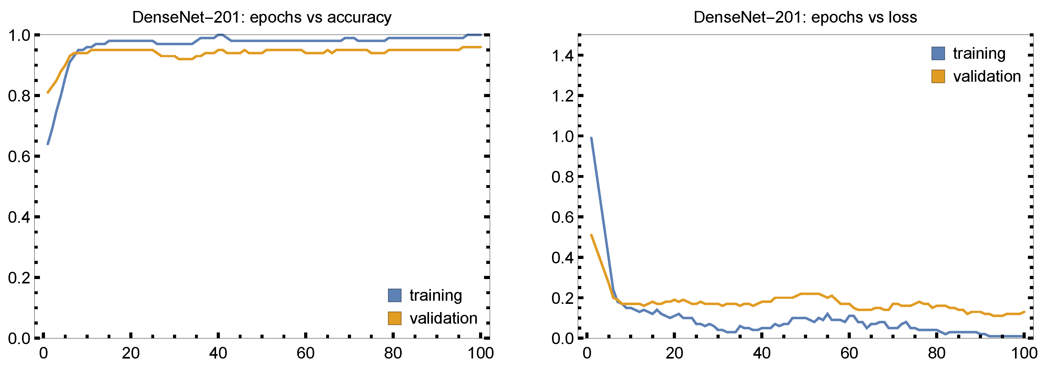
The accuracy of the DenseNet-201 model’s training and validation throughout 100 epochs is plotted in Figure 8. After around 10 epochs, the accuracy stabilizes at values near to 1.00 (i.e., 100%) after increasing during the first few epochs, suggesting that the model quickly picks up on the salient elements of the data. After a few epochs, validation loss stabilizes at low values and the loss curve steadily declines with time. This shows that the model is learning well without overfitting to the training set.

6.5. MobileNet-V2

A lightweight deep learning model called MobileNet-V2 emerged for situations with limited resources. Its design makes use of depthwise separable convolutions to lower computational complexity without sacrificing speed, which makes it a great choice for jobs requiring high accuracy retention combined with high efficiency. A succinct examination of the findings from the MobileNet-V2 model on the dataset is given in the following tables and plots.

The MobileNet-V2 model’s architecture is presented in

Table 13. MobileNet-V2 implementation details.

Layer (Type)	Output Shape	No. of Parameters
MobileNet-V2	(None, 3, 4, 1280)	2,257,984
Flatten (Flatten)	(None, 15,360)	0
Dropout (Dropout)	(None, 15,360)	0
Dense (Dense)	(None, 1024)	15,729,664
Dropout:1 (Dropout)	(None, 1024)	0
Dense:1 (Dense)	(None, 512)	524,800
Dropout:2 (Dropout)	(None, 512)	0
Dense:2 (Dense)	(None, 256)	131,328
Dense:3 (Dense)	(None, 9)	2313
Total parameters: 18,646,089
Trainable parameters: 18,611,977
Non-trainable parameters: 34,112

, which offers a brief overview of the layers, along with the corresponding output shapes and parameter counts. The basis of this model has 2,257,984 parameters, effectively extracting spatial characteristics from the input images. The interspersion of dropout layers prevents overfitting and improves the model’s capacity for generalization. MobileNet-V2 is comparatively light in comparison to deeper designs like DenseNet, which makes the former perfect for deployment in settings like mobile devices where computing resources are quite limited.

The performance MobileNet-V2 at various epochs are shown in

Table 14. MobileNet-V2 parameters and performance.

MobileNet-V2	Accuracy	Precision	Recall	F1 Score	Kappa Score	Test Acc
Epoch: 50	0.9113	0.9133	0.9119	0.9015	0.9138	0.88247
Batch Size: 64
Perclass: 6500
Epoch: 100	0.9441	0.9343	0.9439	0.9349	0.9246	0.9094
Batch Size: 120
Perclass: 8500
Epoch: 120	0.9577	0.9532	0.9473	0.9517	0.9436	0.9185
Batch Size: 150
Perclass: 7500
Epoch: 150	0.9624	0.9536	0.9531	0.9626	0.9646	0.9329
Batch Size: 150
Perclass: 9500
Epoch: 200	0.9673	0.9636	0.9668	0.9696	0.9572	0.9532
Batch Size: 150
Perclass: 6500

, which sheds light on how the model becomes better with additional training. It illustrates how the model performs better over the course of epochs, showing notable increases in test accuracy, recall, accuracy and precision as training goes on. MobileNet-V2 performs almost optimally by Epoch 200 in all measures.

Figure 9 illustrates the accuracy and loss curves for 100 epochs. With a sharp decline in loss over the first 10 epochs and steady, low training and validation losses over the next 10 epochs, MobileNet-V2 exhibits quick learning, good optimization, and little overfitting. Spikes in validation loss do occur, but they have little effect on overall performance. The first few epochs see a sharp increase in accuracy, which reaches 0.90 by Epoch 10. After that, training and validation accuracy steadily climbs and approaches 1.0, indicating robust generalization without overfitting.

6.6. MobileNet-V3 Large

For mobile and edge device deployments, MobileNet-V3 Large is a state-of-the-art model that balances speed and accuracy for maximum efficiency. Using both global average pooling and Dropout layers (with a dropout rate of 0.4) to lessen overfitting while keeping low computational cost, this design is an improvement over earlier MobileNet. By penalizing big weights, L2 regularization is performed to thick layers in this arrangement to help control overfitting. With 1024, 512, and 128 neurons, the dense layers gradually lower dimensionality until the final classification layer uses SoftMax activation to output the prediction for each of the nine skin condition classifications. The smooth convergence during training is ensured by the Adam optimizer, which has a learning rate of 0.0001. Furthermore, adaptive learning is made possible as the model develops by the use of a learning rate reduction method that is triggered by validation accuracy, guaranteeing optimal performance without overshooting. The parameters of this model are given in

Table 15. MobileNet-V3 Large implementation details.

Layer (Type)	Output Shape	No. of Parameters
MobileNet-V3 Large	(None, 3, 4, 960)	2,996,352
GAP 2D	(None, 960)	0
Dropout (Dropout)	(None, 960)	0
Dense (Dense)	(None, 512)	492,032
Dropout:1 (Dropout)	(None, 512)	0
Dense:1 (Dense)	(None, 128)	65,664
Dropout:2 (Dropout)	(None, 128)	0
Dense:2 (Dense)	(None, 9)	1161
Total parameters: 3,555,209
Trainable parameters: 3,530,809
Non-trainable parameters: 24,400

. There are 3,555,209 total parameters, of which 3,530,809 are trainable. The model is efficient and compact despite its complexity.

Table 16. MobileNet-V3 Large parameters and performance.

MobileNet-V3 Large	Accuracy	Precision	Recall	F1 Score	Kappa Score
Epoch: 50	0.9889	0.9887	0.9886	0.9887	0.9875
Batch Size: 32
Per class: 7500
Epoch: 50	0.9803	0.9800	0.9789	0.9793	0.9778
Batch Size: 64
Per class: 7500
Epoch: 100	0.9885	0.9878	0.9870	0.9873	0.9871
Batch Size: 64
Per class: 7500
Epoch: 100	0.9904	0.9898	0.9892	0.9895	0.9892
Batch Size: 128
Per class: 7500
Epoch: 150	0.9897	0.9891	0.9881	0.9885	0.9884
Batch Size: 128
Per class: 7500
Epoch: 200	0.9880	0.9878	0.9871	0.9875	0.9865
Batch Size: 128
Per class: 7500

shows a strong performance throughout epochs. MobileNet-V3 Large attains an accuracy of 0.9889 at Epoch 50, demonstrating quick learning in the early stages of training. The strong recall, accuracy, F1 score, and Kappa scores indicate that each class’s performance is evenly distributed. The accuracy stays high as the training goes on. For example, the model achieves 0.9904 accuracy at Epoch 100, with very little variation in precision and recall between batch sizes. With an accuracy of 0.9880 by Epoch 200, the model continues to perform well, demonstrating that the MobileNet-V3 Large can identify skin lesions accurately and can generalize to data that have not yet been observed.

The accuracy plot in Figure 10 demonstrates that during the first 10 epochs, both training and validation accuracy swiftly converge to values close to 1.00; this suggests that MobileNet-V3 Large can efficiently identify patterns in the dataset early on and keep up a high level of performance during training. Based on the tight alignment of training and validation accuracy, there may not be much overfitting. The loss plot shows that during the first few epochs, especially in the first ten epochs, there is a significant drop in both training and validation loss. Following that, both losses level off at low values, suggesting efficient optimization with minimal error rates. The validation loss occasionally spikes, but they pass quickly and have little effect on overall performance, demonstrating the durability of this model.

6.7. NASNet Mobile

The NASNet Mobile architecture is perfect for mobile applications since it is made to efficiently classify images while keeping a small model size. This model uses the pre-trained NASNet backbone on ImageNet as a feature extractor, with an additional layer to customize it for our classification job. The structure consists of several Dropout layers (with a 0.4 rate) to prevent overfitting, global average pooling to lower the dimensionality of the feature maps, and Dense layers with L2 regularization to further restrict the model’s parameters and enhance generalization. NASNet Mobile employs the Adam optimizer with a learning rate of 0.0001. ReduceLROnPlateau is then used to dynamically modify the learning rate, which aids in optimizing performance throughout training.

Table 17. NASNet Mobile implementation details.

Layer (Type)	Output Shape	No. of Parameters
NasNet (Functional)	(None, 3, 4, 1056)	4,269,716
GAP 2D	(None, 1056)	0
Dropout (Dropout)	(None, 1056)	0
Dense (Dense)	(None, 128)	135,296
Dropout:1 (Dropout)	(None, 128)	0
Dense:1 (Dense)	(None, 64)	8256
Dropout:2 (Dropout)	(None, 64)	0
Dense:2 (Dense)	(None, 9)	585
Total parameters: 44,13,853
Trainable parameters: 437,7115
Non-trainable parameters: 36,738

shows the implementation details.

The tabular findings given in

Table 18. NASNet Mobile parameters and performance.

NASNet Mobile	Accuracy	Precision	Recall	F1 Score	Kappa Score
Epoch: 50	0.9926	0.9927	0.9927	0.9917	0.9804
Batch Size: 32
Per class: 4500
Epoch: 50	0.9997	0.9988	0.9987	0.9977	0.9981
Batch Size: 64
Per class: 4500
Epoch: 100	0.9677	0.9689	0.9706	0.9591	0.9684
Batch Size: 64
Per class: 7500
Epoch: 150	0.9845	0.9846	0.9841	0.9842	0.9825
Batch Size: 64
Per class: 6500
Epoch: 200	0.9921	0.9922	0.9909	0.9915	0.9911
Batch Size: 64
Per class: 7500

demonstrate that the NASNet Mobile model performs at the cutting edge when it comes to complexity and classification accuracy. The classification measures are used to assess the performance over a range of epochs and batch sizes, demonstrating the model’s cross-domain generalization. Precision, recall and F1 score all steadily hold around 0.98, indicating the model’s capacity to reduce false positives as well as erroneous negatives, demonstrating this model’s strong performance in classifying skin lesions accurately. As data augmentation and batch processing become increasingly complicated, the model’s capacity to maintain high performance and good generalization is demonstrated by performance measures across a range of settings.

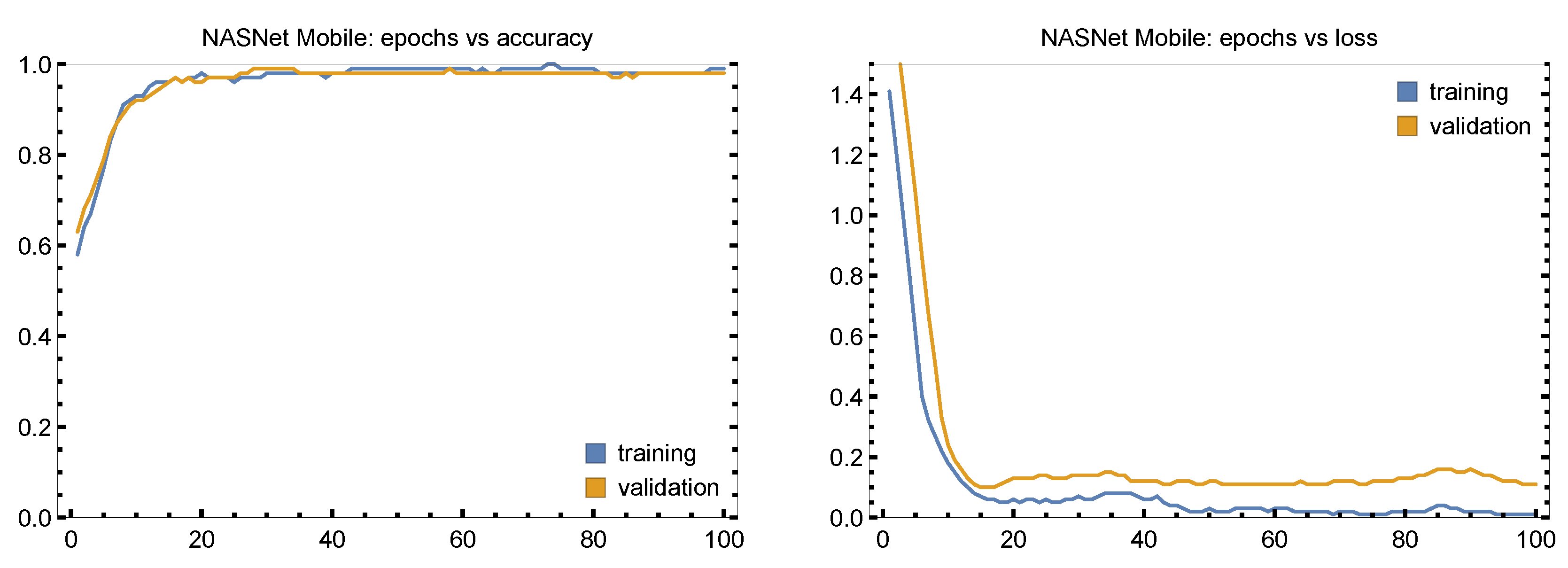
The plots in Figure 11 show a sharp drop in training and validation loss during the first 10 epochs and then consistent, low loss values for the remaining epochs. There are slight variations in validation loss, though these pass quickly, suggesting little overfitting. As with training, validation accuracy rises rapidly as well reaching 0.90 by Epoch 10 and staying continuously near 1.00, which proves the excellent performance of NASNet Mobile on unobserved data and great generalization skills.

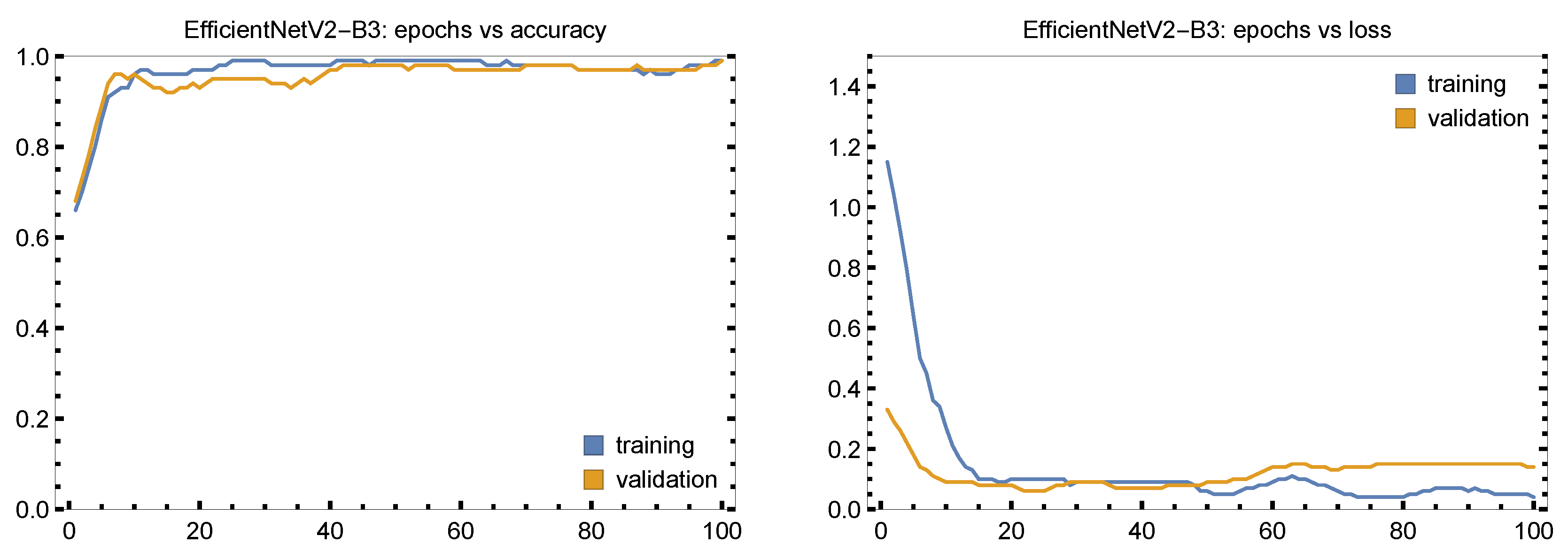
6.8. EffecientNetV2-B3

The EfficientNetV2 architecture is renowned for its effective scalability and performance on big picture classification workloads with comparatively low computing costs. In this instance, L2 regularization has been applied to dense layers, aiding in the regularization of the model, and the model has been optimized using a 0.4 dropout rate to prevent overfitting. By utilizing ReduceLROnPlateau as part of a learning rate reduction approach, the Adam optimizer adjusts the learning rate in accordance with the validation accuracy. This guarantees a steady and regulated learning process all through the instruction. The model’s parameter breakdown is presented in

Table 19. EfficientNetV2-B3 implementation details.

Layer (Type)	Output Shape	No. of Parameters
EfficientNetV2-B3 (Functional)	(None, 3, 4, 1536)	12,930,622
GAP 2D	(None, 1536)	0
Dropout (Dropout)	(None, 1536)	0
Dense (Dense)	(None, 64)	98,368
Dropout:1 (Dropout)	(None, 64)	0
Dense:1 (Dense)	(None, 32)	2080
Dropout:2 (Dropout)	(None, 32)	0
Dense:2 (Dense)	(None, 9)	297
Total parameters: 130,31,367
Trainable parameters: 129,221,51
Non-trainable parameters: 109,216

.

The performance measures for several scenarios are shown in

Table 20. EfficientNetV2-B3 parameters and performance.

EfficientNetV2-B3	Accuracy	Precision	Recall	F1 Score	Kappa Score
Epoch: 50	0.9826	0.9821	0.9822	0.9822	0.9804
Batch Size: 16
Per class: 7500
Epoch: 50	0.9917	0.9918	0.9917	0.9917	0.9907
Batch Size: 32
Per class: 3500
Epoch: 100	0.9624	0.9612	0.9512	0.9718	0.9665
Batch Size: 32
Per class: 7500
Epoch: 150	0.9919	0.9918	0.9917	0.9917	0.9908
Batch Size: 96
Per class: 4500
Epoch: 200	0.9877	0.9880	0.9878	0.9878	0.9861
Batch Size: 64
Per class: 5500

. Both the validation and training accuracy reach 0.90 in the first 10 epochs, indicating a rapid convergence; this implies that the model learns effectively in the early phases and keeps up a high level of performance for the duration of the remaining epochs. After the first 10 epochs, loss levels for both training and validation exhibit a consistent decline that settles at lower values. Low overfitting is shown by the modest divergence between training and validation loss. The validation accuracy closely tracks the training accuracy, indicating strong generalization. The robustness of the model is demonstrated by its strong performance measures over a range of experimental datasets. For instance, 98.26% accuracy with similarly high precision, recall and F1 scores is obtained for Epoch 50 with batch size of 16 and per-class size of 7500 samples, indicating consistent performance across batches and classes.

The accuracy and behavior of the loss curve for 100 epochs are shown in Figure 12. EfficientNetV2-B3 performs well during the whole training procedure. Following ten epochs of fast learning, both the training and validation losses drop off significantly and stabilize at low levels. These two trends stay almost aligned, even if the validation loss is somewhat larger than the training loss, indicating strong generalization without overfitting. Training and validation accuracy rise rapidly, reaching over 90% by the tenth epoch and remain continuously around 98-99%. Although there are some little variations in accuracy and loss, these are transient and have little effect on the model’s overall performance, indicating its effective and steady learning behavior.

7. Confusion Matrices

This section describes the response of all considered models by comparing their respective confusion matrices (Figure 13).

XceptionNet successfully identifies the majority of images in each class, with many diagonal values close to 0.94. Certain classes, such as Mel and BCC, are misclassified based on visual similarity and some forecasts belong to adjacent classes. Given the apparent similarity between several lesion forms, these mistakes in skin cancer categorization are to be expected. Even while this model’s overall accuracy of 0.9481 after 100 epochs, the confusion matrix shows rare misclassifications.

DenseNet-121 properly diagnoses most of the photos across all nine classes as seen by the high values along the diagonal (ranging from 96% to 98%). For example, Mel has a precision of 97.6%, while BCC has a precision of 96.5%. Though infrequent, the misclassifications typically happen between skin cancer kinds that have similar visual characteristics, like BCC and AcKe. In certain instances, this may be due to a modest overlap in visual features. The DenseNet-121 model continues to have excellent discriminative capacity, which supports its usefulness in dermatological image analysis, especially in cases of skin cancer that are relatively prevalent.

DenseNet-169 exhibits strong generalization without appreciable overfitting. Indeed, the diagonal members of its matrix are close to or above 0.95, suggesting that most predictions are correct. This indicates that the model has good recall and accuracy values for all classes. All things considered, this confusion matrix shows that the DenseNet-169 model can effectively discriminate between the many classes of skin conditions, with little misunderstanding between closely related classes.

The DenseNet-201 model performs well across all classes, with excellent classification accuracy. There are very few misclassifications, and the diagonal dominance in its confusion matrix attests to this model’s resilience in accurately recognizing various skin lesions.

With excellent accuracy for the majority of categories, especially Sebok and VL, where classification accuracy surpasses 0.97, the confusion matrix for MobileNet-V2 demonstrates great overall performance across all classes, though closely similar groups like BCC and Mel present a few small misclassifications. The majority of diagonal values for this model are close to or over 0.94, suggesting its ability to discriminate between different skin diseases.

MobileNet-V3 Large performs very well in all classes with the majority of diagonal values being over 0.93, which indicates almost flawless classification accuracy. This model achieves above 0.96 accuracy and performs best with classes like AcKe and BCC. Eventual inaccuracies are small and there is very little misunderstanding among closely similar classifications such as Nev and Sebok.

The confusion matrix of NASNet Mobile shows that this architecture achieves the majority of classes accuracies over 93%. The model’s low off-diagonal values suggest that it performs well in differentiating between various types of skin lesions, such as melanoma and basal cell carcinoma. There is some minor confusion when separating classes like Bas and Mel or Nev and Seb, with little effect on the overall performance of this model.

With the majority of diagonal entries showing accuracies at or above 0.95, the confusion matrix of EfficientNetV2-B3 shows good classification performance across all classes. As evidence of the model’s great generalization skills across the dataset, this demonstrates that the model reliably and highly precisely identifies the proper class.

We observed that architectural features and data sensitivity affected model performance in each experiment. The best generalization and convergence behavior was demonstrated by DenseNet-201 and EfficientNetV2-B3, especially for high-resolution and class-imbalanced datasets. Because of its effective depthwise convolution technique, XceptionNet produced competitive results with a comparatively smaller number of parameters. MobileNet-V3 can be used in field diagnostics because it shown promising accuracy at a greatly reduced resource consumption. These findings highlight how crucial it is to adapt model selection to dataset properties and realistic deployment settings.

8. Conclusions

This research study provides a group of DCNN-based innovative approaches for skin lesion identification and categorization. To boost the system’s performance, we utilized architectures made up of multiple DCNN designs, a series of pre-processing steps and augmentation methods. The proposed DNN algorithms are trained to learn at multiple levels using multiple dense layers and dropout layers, which increases the precision of classification for early-stage skin cancers. XceptionNet, DenseNets, MobileNets, NASNet Mobile, and EfficientNetV2-B3 were among the many CNN models thoroughly evaluated to show how successful deep learning is in challenging multi-class classification tasks. The models were tested on a the open access ISIC with hyperparameters such as batch size, learning rate, and dropout regularization optimized for performance. Confusion matrices, accuracy, and loss plots were used to display the findings, which showed strong categorization efficiency with little overfitting because the validation efficiency closely resembled the training results. DenseNet-201 and MobileNet-V3 Large performed well as well; their capacity to generalize to fresh data was facilitated by dense layers and dropout regularization. The majority of models exhibited consistent validation measures and steady loss curves, demonstrating how well the chosen architectures handled the complexity of the dataset. The EfficientNetV2-B3 and NASNet Mobile models, in particular, achieved the greatest accuracy-to-estimation precision trade-off, which makes them perfect for real-world applications where speed and accuracy are needed. The multi-model statistical measures and excellent findings show the proposed study’s strength in identifying multi-class skin lesions. Additionally, selecting multiple augmentation rates per class improved the understanding of imbalanced data and enabled more accurate detection on a large scale.

Table 21 compares our proposed model with respect to the recent approaches by others in terms of F1 score, precision, accuracy, kappa score, and recall. The closer the given model is to one, the better its classification. Our results prove that all our DCNN algorithms have correctly classified the skin lesions in the images from the ISIC dataset.

The hardware used in this study are the following: NVIDIA Tesla V100 PCIe graphics card, used to perform all computational tasks; 4x Tesla GPU; 2496 cores per GPU; 12GiB GDDR5 VRAM per GPU; CPU Xeon 2.3 GHz (8 dualthread cores); and 64 GiB RAM. It can be seen from Table 5, Table 11, and Table 13 that we have approximately 18 million, 30 million, and 40 million trainable parameters for MobileNet-V2, DenseNet-201, and XceptionNet, respectively, which is less than the up to 266 million trainable parameters reported in the literature [26,33,82]. This study involves using Python 3.8, TensorFlow 2.12, and Keras 2.12 versions.

The models’ lightweight design, especially MobileNet-V2 and NASNet-Mobile, offers great possibilities for deployment on mobile or edge devices, even though they were trained and tested on high-performance GPU computers. Inference times on contemporary smartphones are often between 50 and 100 milliseconds per picture, according to earlier research employing comparable architectures. We plan to concentrate future studies on hardware-specific benchmarks and mobile-optimized models (e.g., TensorFlow Lite and ONNX).

Our models performed extremely well, but they are not intended to take the place of radiologists and dermatologists. Rather, our methodology can benefit physicians by significantly lowering the number of adverse results, which is essential for accurate medical assessment. As a result, we heartily endorse the model for use in helping expert medical specialists identify different types of cancers. This manuscript workflow includes the compilation of skin lesion images, building classification models, enhancing the data to a much larger extent by data augmentation and classifying multi-class images, and can be applied to various medical image analyses, particularly those datasets that have inadequately labeled or intraclass-imbalanced data. This work offers a useful resource for deep learning and AI-based clinical image processing.

Table 21. Comparative analysis of performance metrics of experiments on different datasets by various deep learning techniques, present in the literature along with the proposed study.

Model + Dataset	Precision	Recall	F1 Score	Kappa Score	Accuracy
DCNN + ISIC [83]	0.9048	0.9039	0.9041	—	0.9042
GoogleNet + ISIC [84]	0.8200	0.8000	0.8100	—	0.7306
DenseNet-169 + HAM10000 [85]	0.9295	0.9359	0.9327	—	0.9225
DenseNet-201, SVM + ISBI [47]	0.8824	0.9753	0.9310	—	0.8803
EfficientNet-B4 + HAM10000 [86]	0.8800	0.8800	0.8700	—	0.8802
MultiScale CNN + HAM10000 [87]	0.9640	—	0.7350	—	0.9160
InceptionNet-V3 + ISIC [88]	0.8909	0.9212	0.9223	—	0.9126
DSCC-Net + ISIC [89]	0.9376	0.9428	0.9393	—	0.9417
Random Forest, SVM + ISIC [90]	0.7561	0.8696	0.8089	—	0.8696
CNN + HAM10000 [90]	0.8419	0.8616	0.8600	—	0.8632
Proposed study
XceptionNet + ISIC	0.9639	0.9615	0.9682	0.9738	0.9721
MobileNet-V2 + ISIC	0.9636	0.9668	0.9696	0.9572	0.9673
MobileNet-V3 Large + ISIC	0.9887	0.9886	0.9887	0.9875	0.9889
NASNET Mobile + ISIC	0.9927	0.9927	0.9917	0.9804	0.9926
EfficientNetV2-B3 + ISIC	0.9821	0.9822	0.9822	0.9804	0.9826
DenseNet-201 + ISIC	0.9814	0.9887	0.9823	0.9721	0.9873
DenseNet-169 + ISIC	0.9957	0.9953	0.9955	0.9954	0.9959
DenseNet-121 + ISIC	0.9939	0.9938	0.9938	0.9937	0.9944

Table 21. Comparative analysis of performance metrics of experiments on different datasets by various deep learning techniques, present in the literature along with the proposed study.

Model + Dataset	Precision	Recall	F1 Score	Kappa Score	Accuracy
DCNN + ISIC [83]	0.9048	0.9039	0.9041	—	0.9042
GoogleNet + ISIC [84]	0.8200	0.8000	0.8100	—	0.7306
DenseNet-169 + HAM10000 [85]	0.9295	0.9359	0.9327	—	0.9225
DenseNet-201, SVM + ISBI [47]	0.8824	0.9753	0.9310	—	0.8803
EfficientNet-B4 + HAM10000 [86]	0.8800	0.8800	0.8700	—	0.8802
MultiScale CNN + HAM10000 [87]	0.9640	—	0.7350	—	0.9160
InceptionNet-V3 + ISIC [88]	0.8909	0.9212	0.9223	—	0.9126
DSCC-Net + ISIC [89]	0.9376	0.9428	0.9393	—	0.9417
Random Forest, SVM + ISIC [90]	0.7561	0.8696	0.8089	—	0.8696
CNN + HAM10000 [90]	0.8419	0.8616	0.8600	—	0.8632
Proposed study
XceptionNet + ISIC	0.9639	0.9615	0.9682	0.9738	0.9721
MobileNet-V2 + ISIC	0.9636	0.9668	0.9696	0.9572	0.9673
MobileNet-V3 Large + ISIC	0.9887	0.9886	0.9887	0.9875	0.9889
NASNET Mobile + ISIC	0.9927	0.9927	0.9917	0.9804	0.9926
EfficientNetV2-B3 + ISIC	0.9821	0.9822	0.9822	0.9804	0.9826
DenseNet-201 + ISIC	0.9814	0.9887	0.9823	0.9721	0.9873
DenseNet-169 + ISIC	0.9957	0.9953	0.9955	0.9954	0.9959
DenseNet-121 + ISIC	0.9939	0.9938	0.9938	0.9937	0.9944