Article

Optimal Tuning of Robot–Environment Interaction Controllers via Differential Evolution: A Case Study on (3,0) Mobile Robots

by
Jesús Aldo Paredes-Ballesteros
1,
Miguel Gabriel Villarreal-Cervantes
1,*,
Saul Enrique Benitez-Garcia
1,*,
Alejandro Rodríguez-Molina
2,
Alam Gabriel Rojas-López
1 and
Victor Manuel Silva-García
1
1
Centro de Innovación y Desarrollo Tecnológico en Cómputo, Red de Expertos en Robótica y Mecatrónica, Instituto Politécnico Nacional, Mexico City 07700, Mexico
2
Colegio de Ciencia y Tecnología, Universidad Autónoma de la Ciudad de México, Mexico City 06720, Mexico
*
Authors to whom correspondence should be addressed.
Mathematics 2025, 13(11), 1789; https://doi.org/10.3390/math13111789
Submission received: 30 April 2025 / Revised: 22 May 2025 / Accepted: 26 May 2025 / Published: 27 May 2025
(This article belongs to the Special Issue Artificial Intelligence and Optimization in Engineering Applications)

Abstract

Robotic systems operating in complex environments require optimized tuned interaction controllers to ensure accurate task execution while maintaining smooth and safe behavior. This paper presents a scalarized multi-objective tuning approach based on Differential Evolution (DE) to optimize robot–environment interaction control. The method balances trajectory tracking accuracy and control smoothness using repulsive forces derived from potential fields modeled as virtual springs. The approach is validated on a (3,0) omnidirectional mobile robot navigating predefined trajectories with obstacles. A comparative study of five DE variants shows that DE/best/1/bin and DE/best/1/exp offer the best performance. Simulation and experimental results, including validation with an actual force sensor, confirm the method’s effectiveness and applicability in scenarios with limited sensing capabilities or model uncertainty.

1. Introduction

Robots are dynamic systems designed to assist humans with tasks demanding high precision, significant force, or repetitive and tedious operations. These tasks can be found in activities such as non-invasive surgery [1], handling very heavy loads [2], or mass production of various goods [3]. Robotic systems are composed of several mechanical elements that are related to each other through joints, which can transmit movements of other parts or produce them by employing actuators [4]. Actuators must be properly governed so that robots can perform specific tasks adequately. The control system determines the input signals that enable the robot to accomplish this task [5].
Regardless of their type, all controllers have a set of parameters that determine the robot’s performance in developing its assigned task. The proper configuration of these parameters can enable the robot to complete the assigned task with optimal performance. On the other hand, if the parameters are chosen incorrectly, undesired behaviors may occur, and the task may not be completed effectively. Adjusting these parameters is known as controller tuning [6]. When this process becomes too difficult due to the complexity of the robotic systems, the controller structure, the characteristics of the assigned task, or the performance requirements to be satisfied, using a metaheuristic optimization approach may be convenient [7]. In this approach, an optimization problem is formulated to search for controller parameters that minimize or maximize various performance indicators, which are evaluated based on the robot’s dynamic behavior. The problem is then solved using metaheuristic optimizers. These stochastic algorithms solve complex optimization problems at a reasonable computational cost and are usually inspired by natural, social, or physical phenomena [8].
On the other hand, the arrangement of the robot’s mechanical elements defines its type, such as fixed-base or mobile-base configurations. Fixed-base robots are anchored in a fixed point and are valuable in industrial environments for performing pick-and-place operations within workspaces defined by their mechanical components’ reach and range of motion [9]. In contrast, mobile robots can extend their workspace by repositioning their base, allowing them to operate beyond the stationary range of fixed-base robots [10]. Mobile robots have significantly expanded to address the increasing demand for goods and passenger transportation [11], exploration of unknown environments [12], and critical operations such as surveillance, search, and rescue [13]. Among these robots, the omnidirectional ones have recently gained prominence due to their ability to move in any direction regardless of their orientation [14]. This unique capability makes them particularly well-suited for confined or high-traffic environments where maneuverability and precise positioning are crucial, such as warehouse navigation and manipulation [15].
No matter their type, the environments in which robots operate are becoming increasingly diverse and complex [16,17]. These environments often feature obstacles such as people [18], other robots [19], different objects [20], or living beings [21]. Consequently, it is essential to equip robots with capabilities that allow them to interact effectively with these elements, ensuring they complete their tasks efficiently while minimizing disruptions to their surroundings. These capabilities relate to how robots acquire information about obstacles or collisions with obstacles and how they implement a force controller to best respond to these interactions [22].
The interaction between robots and their operating environment can be determined in two ways: by using direct measurements of the force sensors in the system or by making approximations based on other measurements. In the first case, the force with which a robot interacts with the objects in its environment is measured when direct contact is encountered [23,24], and the information from this measurement can be incorporated into the controller to adjust its behavior [25]. The above is useful when high accuracy is required in measuring the physical interaction, and force sensors are affordable. In the second case, the interaction force is estimated from other measurements (e.g., distance, speed, acceleration, motor torque or current, pressure, or structural deflections or deformations) without direct contact and then incorporated into the force control [26,27,28,29]. Estimates are convenient when it is desired to avoid direct contact or when force sensors are unavailable.
Regardless of whether the force value is directly measured or estimated, it is incorporated in the force control to modify the robot’s behavior depending on its interaction with the environment, either to regulate the force it applies; to adjust the trajectory for avoiding the collision; to change its position, speed or acceleration causing smoother interactions; or to compensate for the impact of external forces to complete the desired task without deviating too much.
In direct force control, the force measured or estimated is compared against a desired force to obtain an error used during the control signal calculation [30]. Likewise, there are hybrid position and force controls, where in addition to the regulation of the force intensity, the error is also considered in the calculation of the control signal of the robot for the performance of tasks such as assembly, parts insertion, or scanning, which involve movements and physical contact with the environment [31]. Impedance or admittance controls simulate the behavior of a passive mechanical system (usually a mass-spring-damper system) to promote smooth interactions between the robot and its environment, i.e., to handle or repel collisions or contacts smoothly, avoiding abrupt reactions that may cause damage [32,33]. Finally, external force compensation controllers aim to eliminate the effects of external forces by applying an opposing action to cancel them, allowing the robot to follow its desired trajectory with minimal disturbance [34].
As with any other controller, the force controllers of all the types described above have parameters that compromise the robot’s performance in achieving the established task. In force controllers, control gains, filters, physical parameters of the mass-spring-damper system models, or of the dynamic models of the system that estimate forces, etc., are tuned [35,36,37].
The demands of today’s systems require robots to meet broader operational requirements, beyond simply performing a task with minimal error, by responding with appropriate actions when interacting with the environment. In this sense, controller tuning can be naturally modeled in mathematical language as an optimization problem where the value of the design variables, i.e., the controller parameters, is minimized concerning one or several objective functions. These functions evaluate the level of compliance with the operational requirements related to the correct performance of the established task or the adequate interaction with the environment. Moreover, the variables may be constrained to avoid undesired dynamic behaviors [7].
Optimization problems related to force controller tuning exhibit varying complexities, influenced by the characteristics of the controller, the controlled system, and the environment, and are generally challenging to solve. That is why metaheuristics are frequently used in the specialized literature as solvers to the force controller tuning problem. Metaheuristics, such as Particle Swarm Optimization (PSO), Genetic Algorithms (GA), and Differential Evolution (DE), have been effectively used for force-based controller tuning in various robotic applications. In [38], PSO optimizes the parameters of an adaptive impedance controller, improving the system response to variations in the environment. The study in [39] combines Particle Swarm Optimization (PSO) with Graph-based Knowledge Transfer (GKT) to adjust the force control in a massage robot, thereby adapting to the varying dynamics of human skin. In [40], GA optimizes the trajectories of a robotic arm, improving force control during the drawing process. In [41], DE tunes the Active Disturbance Rejection Controller (ADRC) in a bearingless motor, enhancing its ability to adapt to external disturbances. The work in [42], which utilizes a Fuzzy-PID controller, optimizes a vehicle’s semi-active suspension using DE, thereby tuning the controller gains in real-time to enhance ride comfort. Finally, ref. [43] combines impedance control and genetic algorithms (GA) to optimize the robotic grinding trajectory, thereby improving force control in the surface finishing process.
To this point, it can be seen that the challenges faced by robotics systems interacting with the environment include adaptability to dynamic changes in the environment, accurate tuning of controller parameters, maintaining stable and efficient control in the face of external disturbances, and smooth and accurate interaction with the environment, ensuring robust performance under varying conditions. However, most existing work on interaction controller tuning focuses primarily on minimizing trajectory tracking errors without adequately considering the smoothness of the control signal, an essential factor for safe and efficient interactions. In addition, many approaches rely heavily on direct force sensing or very accurate physical models, which limits their feasibility in dynamic or resource-constrained environments. Therefore, there is a clear need for reliable tuning methods that integrate virtual force sensing and optimization of different control criteria simultaneously, addressing both performance and smoothness of the interaction in realistic scenarios.
This study introduces a tuning approach for robot–environment interaction controllers that leverages repulsive forces numerically derived from virtual potential fields through a spring-like model. This approach enables real-time obstacle avoidance and trajectory correction to address these challenges. The Proportional-Derivative controller with Gravity compensation (PD+G controller) is optimized using a scalarized multi-objective approach that minimizes the trajectory tracking errors while ensuring smooth and responsive control actions. To achieve this, variants of the metaheuristic algorithm known as Differential Evolution (DE) [44] are employed for their robustness and efficiency in solving complex optimization problems.
The proposed controller tuning approach for robot–environment interactions is evaluated on a (3,0) mobile robot (an omnidirectional one) [45] that follows a predefined trajectory within a limited time frame while encountering a single obstacle. A statistical comparison of different DE variants identifies the most effective solver for the optimization problem. Additionally, the DE-optimized controller is benchmarked against an alternative tuning approach, demonstrating a superior balance between the trajectory tracking accuracy and the control signal smoothness.
The main contributions of the work are summarized as follows: (i) The first one is the formulation of the controller tuning approach for robot–environment interaction tasks, where the tracking error and the controller smoothness are simultaneously optimized. It presents a systematic approach for tuning controller parameters of robotic systems using a scalarized multi-objective optimization approach with differential evolution variants serving as solvers. The proposal incorporates virtual repulsive forces into the controller to numerically simulate the influence of obstacles. The controller’s stability analysis demonstrates the relationship between the repulsive force and the controller gains, enabling stable robot behavior in the presence of obstacles within the environment. Notably, the optimized gains not only work with virtual forces but also effectively perform when applied to a real force-sensing system, demonstrating the practical applicability of the approach in real-world scenarios and its robustness under various robot–environment interactions. To the best of the authors’ knowledge, this is the first time that interaction controllers have been optimized with a spring-like repulsive force model and that gains have been validated in a real force-sensing system. (ii) The second contribution is the application of the proposed controller tuning approach to a (3,0) mobile robot, revealing the proposal’s effectiveness in simulation and experimentation. It also provides information about the most promising DE variants, which could help practitioners or researchers select effective optimization strategies in similar controller tuning tasks.
The remainder of this paper is organized as follows. Section 2 formulates the proposed controller tuning approach for robot–environment interactions as a dynamic optimization problem for the general robot dynamics. The proposal’s application to the (3,0) mobile robot is also presented. Section 3 describes the most representative DE variants that solve the case study. The obtained results and the corresponding discussions are given in Section 4. The conclusions are drawn in Section 5.

2. Controller Tuning Approach for Robot–Environment Interactions Based on Differential Evolution Optimizers

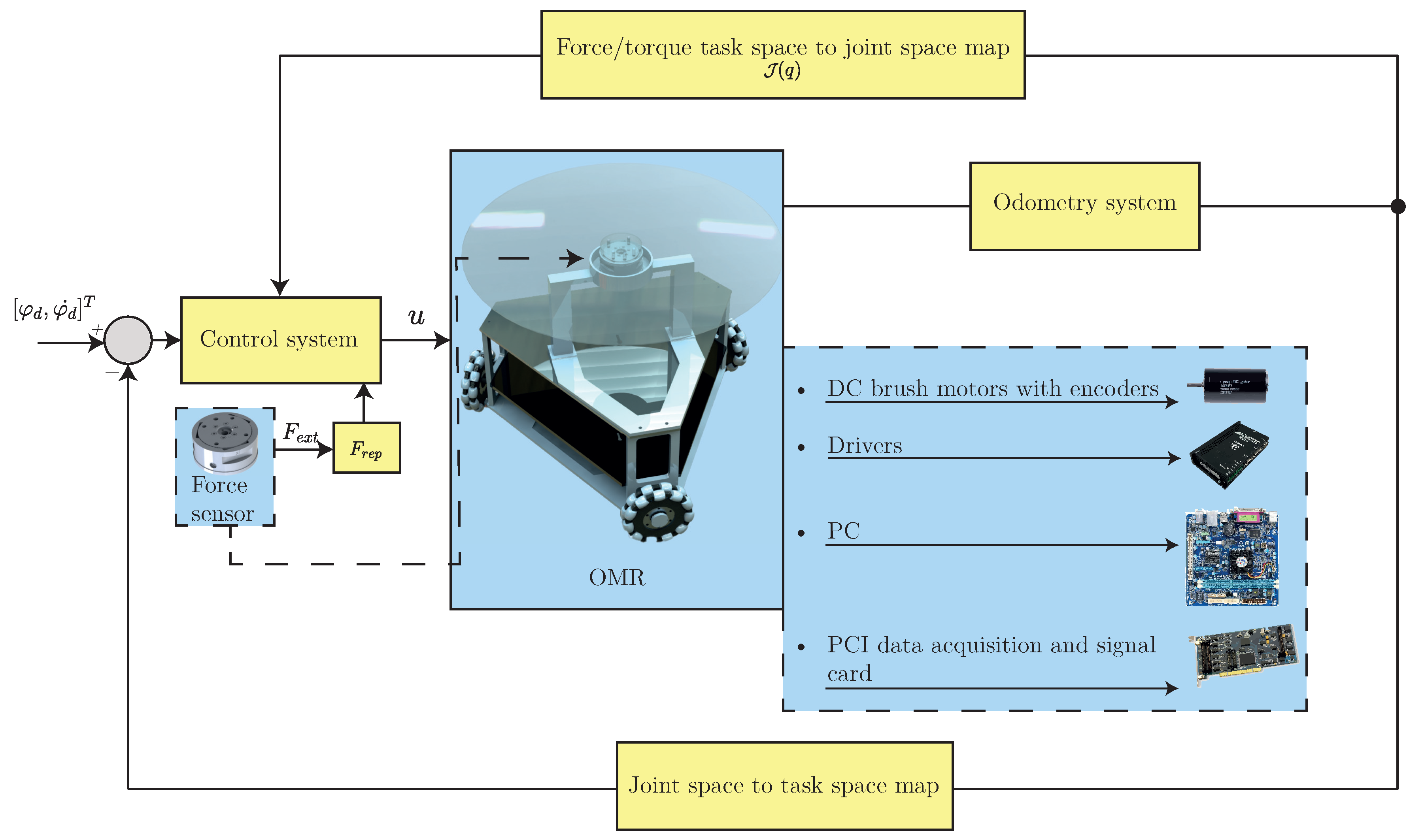
2.1. Robot Dynamics and Control System

Consider the robotic system dynamics described by (1), where M ( q ) R n × n is the definitive positive symmetric inertia matrix, C ( q , q ˙ ) q ˙ R n is the Centrifugal and Coriolis force vector, G ( q ) R n is the gravity force vector, τ R m is the input force/torque vector, q , q ˙ , q ¨ R n are the position, velocity and acceleration of the generalized coordinates in the joint space that describes the robot behavior. It is assumed that the robot is fully actuated and is not redundant.
M ( q ) q ¨ + C ( q , q ˙ ) q ˙ + G ( q ) = τ
The chosen control system τ = u is provided in (2), where K p = d i a g ( k p 1 , , k p n ) , K d = d i a g ( k d 1 , , k d n ) R n × n are diagonal matrices with the proportional and derivative gains, respectively, the position error vector and the velocity error vector in the task space (Cartesian space) are given by e φ = φ d φ R n , e ˙ φ = φ d ˙ φ ˙ R n , respectively, φ , φ ˙ R n are the position and velocity vectors of the robot’s end-effector in the task space (Cartesian space), φ d , φ d ˙ R n are the desired position and velocity vectors of the robot’s end-effector in the task space, J R n × n is the Jacobian matrix relating the space from q ˙ to φ ˙ and F r e p R n is the perception of the force exerted by the robot–environment interaction named in this work as the repulsive force vector.
u = J T ( K p e φ + K d e ˙ φ + F r e p ) + G
The closed-loop system of the dynamics (1) with the controller (2) for the regulation problem is presented in (3), and the schematic diagram is shown in Figure 1.
M q ¨ + C q ˙ J T ( K p e φ K d φ ˙ + F r e p ) = 0
It is observed when F r e p = 0 , the equilibrium point is the origin [ e φ , φ ˙ ] = [ e φ , q ˙ ] = [ 0 , 0 ] . Otherwise, when F r e p 0 , the equilibrium point is [ e φ , φ ˙ ] = [ e φ , q ˙ ] = [ K p 1 F r e p , 0 ] .
  • Stability Analysis
Consider the candidate Lyapunov function presented in (4).
V ( e φ , q ˙ ) = 1 2 q ˙ T M q ˙ + 1 2 e φ T K p e φ
The derivative of (4) is given as
V ˙ ( e φ , q ˙ ) = q ˙ T M q ¨ + 1 2 q ˙ M ˙ q ˙ e φ T K p φ ˙
Substituting the closed-loop system (3) in (5), and considering the map J from the joint velocity vector q ˙ to the Cartesian velocity vector φ ˙ and using the robot dynamic property 1 2 q ˙ T M ˙ q ˙ q ˙ T C q ˙ = 0 results:
V ˙ ( e φ , q ˙ ) = q ˙ T ( J T ( K p e φ K d φ ˙ + F r e p ) C q ˙ ) + 1 2 q ˙ T M ˙ q ˙ e φ T K p φ ˙ = q ˙ T J T K d φ ˙ + q ˙ T J T F r e p
Using the La Salle theorem to find { [ e φ , q ˙ ] | V ˙ = 0 , [ e φ , q ˙ ] = [ 0 , 0 ] } , it is clear that when F r e p = 0 , the function V is a Lyapunov one and hence, the equilibrium point is the origin [ e φ , q ˙ ] = [ 0 , 0 ] and is an asymptotically stable equilibrium point. Otherwise, when F r e p 0 the closed-loop system converge to [ e φ , q ˙ ] = [ K p 1 F r e p , 0 ] , indicating that the repulsive force F r e p repel the equilibrium point from the origin due to the existence of robot–environment interactions (the perception of obstacles). Once the obstacle is avoided, the equilibrium point converges to the origin.

2.1.1. Repulsive Force as a Potential Field

This section introduces the concepts necessary for developing the repulsive force in the control strategy described in Section 2.1. Some definitions related to potential fields will be set for this case. Potential fields U have frequently been used in path planning for robots. The basic idea of potential field approaches is to construct potential fields in the space Ω where the robot’s task is carried out (in this case, the Cartesian space), such that the point of interest where the robot’s task will be performed is attracted to the goal φ f i n a l and repelled from the obstacle region Ω ¯ . Generally, the potential field U is composed of the sum of attractive and repulsive potentials, where the gradient of the potentials U indicates the most promising local direction for movement in path planning. Consider φ Ω ; the potential field U ( φ ) is given by (7).
U ( φ ) = U a t r ( φ ) + U r e p ( φ )
The repulsive potential field is interesting in this work because the controller (2) requires repelling the obstacle by F r e p in the path, allowing the end-effector to complete the desired task. So, the attractive one is not described in the next section.

2.1.2. Repulsive Potential Fields

The repulsive potential field must keep the point of interest in the robotic system away from obstacles, preventing the robot from colliding. When the robot is sufficiently far from obstacles, the potential field should not influence the robot’s movement.
For the particular case, the following repulsive potential field (8) is proposed, where its gradient provides the repulsive force (9) required to repel obstacles.
U r e p ( F e x t ) = 1 2 η ρ ( F e x t ) 2 , if ρ ( φ ) > 0 0 , if ρ ( φ ) = 0
F r e p ( F e x t ) = η ρ ( F ext ) ρ ( F e x t ) = η F ext , if ρ ( φ ) > 0 0 , if ρ ( φ ) = 0
The terms associated with the above equations are: the external force and torque vector generated by the collision with the obstacle is F e x t R n , the external resultant force is given by ρ ( F e x t ) = F e x t R , ρ = F e x t F e x t R n is the gradient vector of external forces and torques generated upon colliding with an obstacle, and η = diag { η 1 , , η n } R n × n is a diagonal matrix with the scalar gain coefficients that determine the influence of the repulsive field.
The external resultant force of F e x t (force generated by the collision between the robot and the obstacle) is numerically simulated using a spring-like model, as shown in Equation (10). The terms of (10) are described as follows: K is the vector containing the stiffness constant, b is the vector representing the geometric center position of the obstacle, φ is the robot position in the task space, λ 0 is the influence distance of the obstacle (circle radius containing the obstacle), ϵ is the influence distance of the robot (circle radius containing the robot) and λ is the distance between the geometric centers of the obstacle and the robot, as illustrated in Figure 2. It is important to point out that the external force is applied ( F e x t 0 ) when a collision occurs, i.e., when λ = b φ λ 0 + ϵ . Otherwise, when the robot does not collide with the obstacle (the distance λ is larger than the influence distances λ 0 and ϵ ), there is no external force, i.e., F e x t = 0 .
F e x t = K ( b φ ) ( sign ( λ λ 0 ϵ ) 1 ) 2

2.2. Optimization Problem Formulation

Once the controller to be implemented is defined, the criteria to optimize are described to improve the robot’s closed-loop system performance. The control parameters K p and K d are grouped in the design variable vector p R 2 n to improve the objective function.
The first criterion to optimize is the mean of the Integral of the Squared Error (ISE) [46,47] to reduce the components of the task space position error e φ , as is observed in (11), where t f is the final time.
J 1 = 1 t f 0 t f e φ T e φ d t
The second criterion to optimize is the mean of the Absolute Value Integral Square of the Derivative Control Signal (ISDU) [48]. The ISDU metric assesses the smoothness and behavior of the control signal, aiming to regulate it smoothly in the event of a collision. To achieve this, the functional presented in (12) is proposed, aiming to minimize the difference between the control signals at the current time t and those computed at the previous time t d t .
J 2 = 1 t f 0 t f u ( t ) u ( t d t ) 2 d t
It is important to point out that with the inclusion of the repulsive force ( F r e p 0 ), the control signal u can exceed the maximum torque/force delivered by the physical motor. To limit the search of the optimization process and create a more realistic scenario, the control signal u is constrained to its physical limits, u m a x and u m i n , when it is computed.
By transforming the multi-objective problem into a single-objective one through the weighted sum method [49], the objective function to minimize is given by (13). By assigning values to the weights μ 1 and μ 2 , the priority to improve the corresponding functional is set. The greater the weight, the higher the priority for minimization. It is essential to note that the objective function incorporates a normalization process, where each function is scaled to its maximum possible value to mitigate issues arising from physical quantity differences. So, J 1 max , J 2 max are the maximum value that J 1 , J 2 can reach when each term is separately minimized, representing the worst possible performance in terms of the criterion evaluated. That is, since the proposed controller tuning approach for robot–environment interactions is formulated offline, the maximum value of each objective term J j is estimated through numerical simulations by individually minimizing J i and subsequently evaluating J j using the optimal design variables obtained from the minimization of J i , for all j i .
J = μ 1 J 1 J 1 m a x + μ 2 J 2 J 2 m a x
On the other hand, it is important to include the physical limitations that the robot is subject to. The first constraint is given by its dynamics, represented in state-space form as χ ˙ = f χ ( χ ) g χ ( χ ) u with its state initial condition χ i n i . Including the noise introduced in the output signal by the control signal is crucial because, in a real environment, this could perturb the controller’s performance. Then, Gaussian noise is added to the controller’s computation to simulate a real environment. The Gaussian random number value ξ in the interval [ 0.0001 , 0.0001 ] affects each generalized coordinate and velocity in the closed-loop simulation, i.e., the controller (2) is described by u = f u ( p , χ + ξ ) . Similarly, the control signal is limited to the physical power source in a real environment. So, the control signal is bound to its maximum value u m a x when its limit is surpassed in the execution of the closed-loop system. The second constraints are related to the limits of the design variable vector, where p m i n and p m a x are the minimum and maximum bounds of the search region.
Thus, the dynamic optimization problem addressed in this work (14)–(16) for the controller tuning approach for robot–environment interactions finds the control design variable vector p R 2 n that minimizes the performance function J R (13), subject to the closed-loop system dynamics with its initial conditions χ ( 0 ) = χ i n i (15) and the bounds in the design variable vector (16).
min p R 6 J ( p ) s . t .
χ ˙ = f ( χ ) g ( χ ) u ( p , χ + ξ ) ; χ ( 0 ) = χ i n i
p m i n < p < p m a x

2.3. Case Study: Application to Omnidirectional Mobile Robots

In this case study, the omnidirectional mobile robot (OMR) is selected as the subject to validate both simulated and experimental implementations of proposed controller tuning based on optimization given in (14)–(16).
The schematic representation of the OMR is described in Figure 1. The wheel’s location forms an equilateral triangle because this configuration maximizes the dexterity in the task space [50]. The parameters that encompass the mechanical, kinematic, and dynamic aspects of the OMR are listed in Table 1. The OMR is considered under the assumption that it is placed on a flat horizontal surface, with no friction involved, and with non-deformable wheels. Two coordinate frames are considered: ( X w , Y w ) , representing the world coordinate frame, and ( X m , Y m ) , assigned to the OMR coordinate with its origin at the center of mass, m, and moment of inertia, I z . An angle of ϕ w rotates the OMR’s frame concerning the world frame (Figure 3).
The closed-loop dynamics of the OMR considering the representation of the system given by [51] for preserving the structural properties of the robot model is presented as M ( q ) q ¨ + C ( q , q ˙ ) q ˙ = B ¯ u , with the terms described by (17)–(19) and using the generalized coordinates q = [ x w , y w , ϕ w ] T and their velocities q ˙ = [ x ˙ w , y ˙ w , ϕ ˙ w ] T . The matrix R m w ( ϕ w ) relates the rotation of one of the mobile robot frames to the world frame (Cartesian space).
M = R m w 2 m r 2 + 3 J 2 r 2 cos ϕ w 2 m r 2 + 3 J 2 r 2 sin ϕ w 0 2 m r 2 + 3 J 2 r 2 sin ϕ w 2 m r 2 + 3 J 2 r 2 cos ϕ w 0 0 0 3 J L 2 r 2 + I z
C = R m w 3 J 2 r 2 ϕ ˙ w sin ϕ w 3 J 2 r 2 ϕ ˙ w cos ϕ w 0 3 J 2 r 2 ϕ ˙ w cos ϕ w 3 J 2 r 2 ϕ ˙ w sin ϕ w 0 0 0 0
B ¯ = R m w 3 2 r 0 3 2 r 1 2 r 1 r 1 2 r L r L r L r
The dynamic of the OMR is represented by the following state-space system χ ˙ = f ( χ ) g ( χ ) u with the state vector expressed as χ = [ x w , y w , ϕ w , x ˙ w , y ˙ w , ϕ ˙ w ] T R 6 and the system terms defined in (20) and (21), where λ ¯ = 1 2 m r 2 + 3 J L , κ ¯ ± = sin x 3 ± 3 cos x 3 , and ψ ± = cos x 3 ± 3 sin x 3 .
f ( x ) = χ 4 χ 5 χ 6 3 J λ ¯ χ 6 χ 5 3 J λ ¯ χ 4 χ 6 0 T R 6
g ( x ) = 0 0 0 0 0 0 0 0 0 λ ¯ r κ ¯ 2 r λ ¯ sin χ 3 λ ¯ r κ ¯ + λ ¯ r ψ + 2 r λ ¯ cos χ 3 λ ¯ r ψ λ ¯ r ψ + 3 J L 2 + I z r 2 2 r λ ¯ cos χ 3 3 J L 2 + I z r 2 λ ¯ r ψ 3 J L 2 + I z r 2 R 6 × 3
A circle in the Cartesian space is selected as the trajectory to be followed by the OMR, considering that there is no rotation in the OMR orientation. The desired trajectory is expressed as χ ¯ = [ x ¯ w , y ¯ w , ϕ ¯ w , x ˙ ¯ w , y ˙ ¯ w , ϕ ˙ ¯ w ] T R 6 and characterized by the Equation (22). In this representation, x c and y c define the center of the circular trajectory, r t its radius, and t the current time.
χ ¯ = x c + r t cos ( 2 π f t t ) y c + r t sin ( 2 π f t t ) 0 2 π f t r t sin ( 2 π f t t ) 2 π f t r t cos ( 2 π f t t ) 0
In this case, a stationary circular object is the obstacle with which the OMR collides. This is described by the parametric equations presented in (23) and illustrated in Figure 2. The parameter λ 0 , which is also interpreted as the distance of influence, corresponds to the radius of the obstacle. Additionally, the vector b = ( b x , b y , b ϕ ) represents the geometric center of the obstacle’s position. In this particular case, the first two positions of the vector b are related to the center of the circle in the Cartesian space, and the last one represents its orientation limit. The obstacle position is provided by ( x o , y o , ϕ o ) .
( x o b x ) 2 + ( y o b y ) 2 = λ 0 2 ϕ o = b ϕ

3. Optimization Techniques

The algorithm selected to address the optimization problem posed in (14) is Differential Evolution (DE). DE is based on a stochastic process and is used to solve nonlinear optimization problems [52]. Initially proposed by Kenneth Price and Rainer Storn in [44], this algorithm is inspired by the evolutionary process of species, with the primary aim of finding an optimal solution from a population through the evolution of generations, where the population represents the various possible solutions to an optimization problem defined within a search space. Through generations (iterations), the population adapts and converges or evolves towards an optimal solution through a process of mutation and crossover, selecting the most suitable solution. It is noteworthy that for this work, DE is used with different variants, considering its effectiveness in controller tuning problems [53]. This approach is particularly relevant, given that DE has been applied in OMR [45,54].
The pseudocode for DE is presented in Algorithm 1, where the design variable vector p is included in x, i.e., x = p . The following are the four defined stages that make up the algorithm:
Algorithm 1 Pseudocode
Require: Maximum generations ( G m a x ), Population size ( N P ), Bounds ( [ x m i n , x m a x ] ), Crossover rate ( C R ), Scaling factor ( [ F m i n , F m a x ] ).
Ensure: Best solution x * .
 1:
G 0
Initialization stage:
 2:
Create initial population X G of N P individuals, where each individual is randomly generated x [ x m i n , x m a x ] .
 3:
Evaluate for each individual in J ( x i G ) i 1 , , N P .
 4:
while  G < G m a x   do
 5:
    for each  x i  in  X G  do
 6:
         Randomly obtain F [ F m i n , F m a x ] .
 7:
         Randomly select three individuals from the population, such that x r 1 x r 2 x r 3 x i X G .
         Mutation and crossover stages:
 8:
         Generate a new individual u G i using mutation and crossover from DE given in Table 2.
 9:
         Evaluate J ( u G i ) .
         Selection stage:
10:
        if  u G i  is better than  x G i  then
11:
            x G + 1 i = u G i
12:
        else
13:
            x G + 1 i = x G i
14:
        end if
15:
    end for
16:
     G G + 1 .
17:
end while
  • Initialization
At the beginning of the algorithm, a random initial population X G R N P × D of N P individuals x i G R D i { 1 , , N P } is created. Each individual in the population X G represents a candidate solution in generation G to the optimization problem. It is important to note that all individuals are within a space bounded by lower and upper limits x [ x m i n , x m a x ] . Afterward, the fitness of the population’s individuals is evaluated by computing the objective function J ( x i ) with the design variables of each individual in the population X G .
  • Mutation
The mutation is the operator used to introduce genetic diversity into the candidate solutions. This allows for the exploration of new regions of the search space, thanks to the scale factor F [ 0 , 1 ] , where higher values of F produce larger mutations, and lower values result in smaller mutations. The scale factor is usually multiplied by the difference between two randomly chosen individuals x r 1 x r 2 x r 3 x i X G , all of which are added to the best x b e s t in the case of best DE variant, random x r 3 in the case of rand DE variant, or current individual x i with an arithmetic crossover in the case of current-to-rand DE variant as shown in Table 2. Mutation mimics the concept of random changes in each of the new solutions to explore new regions of the search space.
  • Crossover
The crossover operation in differential evolution combines a parent individual x i G with a mutated individual v to produce a new offspring u i G . This process is controlled by the crossover factor C R , which regulates the exchange of information between individuals. A low C R value promotes a more focused search by exploiting existing information, while a high value encourages exploration in the search space. In binomial and exponential crossover, new individuals are selected based on a probabilistic condition, choosing between mutated and original values. In the binomial crossover, the new value v j i is selected randomly, i.e., if rand j ( 0 , 1 ) < C R or if j equals a randomly chosen index j rand . This introduces randomness for exploration. In the exponential crossover, the selection condition remains active throughout the process, allowing a set of components to transfer to the child vector while rand j ( 0 , 1 ) < C R is satisfied or if j = j rand , offering an exploitative search for generating new individuals with more similarities than the binomial crossover.
  • Selection
At this stage, the individual (between parent and offspring) that will pass to the next generation G + 1 is chosen using (24). In this case, the individual with the most promising performance function, whether between the parent and the offspring, is selected.
x G + 1 i = u G i if J ( u G i ) J ( x G i ) x G i otherwise
Table 2. Mutation and crossover operators of DE.
NomenclatureVariant
DE/rand/1/bin u i j = v j i = x j r 3 + F ( x j r 1 x j r 2 ) if rand j ( 0 , 1 ) < C R or j = j rand x i j otherwise
DE/rand/1/exp u i j = v j i = x j r 3 + F ( x j r 1 x j r 2 ) while rand j ( 0 , 1 ) < C R or j = j rand x i j otherwise
DE/best/1/bin u i j = v j i = x j b e s t + F ( x j r 1 x j r 2 ) if rand j ( 0 , 1 ) < C R or j = j rand x i j otherwise
DE/best/1/exp u i j = v j i = x j b e s t + F ( x j r 1 x j r 2 ) while rand j ( 0 , 1 ) < C R or j = j rand x i j otherwise
DE/current-to-rand/1/bin u i j = v j i = x j i + K ( x j r 3 x j i ) + F ( x j r 1 x j r 2 ) if rand j ( 0 , 1 ) < C R or j = j rand x i j otherwise
At the end of the optimization process, the algorithm identifies the best solution from the individuals within the final population, the solution that most reduces the objective function, denoted by the set X G . This procedure facilitates the selection of the individual that most closely satisfies the objective function, ensuring that the best solution is found after the optimization process.

4. Results

In this work, evolutionary optimization aims to significantly enhance the controller tuning performance of omnidirectional mobile robots in robot–environment interactions. For this purpose, tests of the proposed controller tuning are conducted in numerical simulations and experimental environments. The following sections detail these results and provide a comprehensive overview of both the numerical simulations and the experimental tests.

4.1. Optimization Process Conditions

This section describes the conditions for the offline controller tuning process shown in Figure 1, where numerical simulations of the controller for the OMR are carried out using parameters that encompass mechanical, kinematic, and dynamic aspects of the OMR, as shown in Table 1.
The simulation time interval spans from t 0 = 0 to t f = 210 s with an integration time of Δ t = 5 ms. During this period, the OMR must follow a circular trajectory χ ¯ (22) with a center at the origin, a radius of r t = 1 m and a frequency of f t = 210 Hz. The initial condition vector of the OMR is set as x ( 0 ) = [ 1 , 0 , 0 , 0 , 0 , 0 ] T . The circular obstacle (23) is located in the Cartesian coordinate b = [ 0.7 , 0.7 ] with an influence distance λ 0 = 0.28 . Regarding the repulsive force F r e p described by (9), the diagonal elements of the matrix η are set to η = diag ( 250 , 250 , 0 ) . The stiffness constant of the spring that emulates the associated external force F e x t is given by K = diag ( 2 , 2 , 0 ) with φ = [ x w , y w , ϕ w ] and the robot’s influence distance ϵ = L = 0.287 m.
The conditions of the optimization process in the proposed control tuning strategy are presented below. The following five DE variants were selected: DE/rand/1/bin, DE/rand/1/exp, DE/best/1/bin, DE/best/1/exp, DE/current-to-rand/1/bin, as described in Section 3, under the following algorithm parameters: a population size of N P = 60 individuals, evolving over G m a x = 300 generations, with a crossover coefficient of C R = 0.6 , a random scaling factor F [ 0.3 , 0.9 ] , and the search space bounded by a lower limit p m i n = [ 0 , 0 , 0 , 0 , 0 , 0 ] T R 6 × 1 and an upper limit p m a x = [ 100 , 100 , 100 , 100 , 100 , 100 ] T R 6 × 1 . The previous algorithm parameter settings were chosen by analogy [55], adopting values that were successful in similar previous works. Additionally, the weight values μ 1 = 0.99 and μ 2 = 0.01 were selected “by hand” [55], where different algorithm parameter configurations are tested, and the most suitable tradeoff is considered. In this particular case, assuming that μ 1 + μ 2 = 1 , initial sweeps of the weight values are performed by varying μ 1 from 0.1 to 0.9 in steps of 0.1 ( 10 % of variation) to identify the region of interest in which the performance function J, composed of the terms J 1 (tracking error) and J 2 (control effort smoothness), showed promising tradeoffs. Once this region is found, finer sweeps of the weight values are carried out using increments of 0.002 in μ 1 within the range ( [ 0.982 , 0.998 ] ) ( 0.2 % of variation) to refine the weight selection. This refinement aids in the selection of a weight configuration that offers a favorable compromise between trajectory tracking accuracy and control signal smoothness. Figure 4 presents the sensitivity analysis in the weight variations with respect to the terms J 1 and J 2 of the performance function J. The filled circle represents the Pareto solutions (PSs), whereas the open circles are solutions that the PSs dominate. The star denotes the PS selected. This figure illustrates that increasing μ 1 improves tracking accuracy at the expense of control smoothness, and vice versa. The chosen weight configuration reflects a deliberate preference toward minimizing the tracking error while maintaining acceptable smoothness in the control effort. This analysis not only validates the chosen weight values but also supports the effectiveness of the proposed scalarization strategy in balancing the performance function terms.
Thirty independent executions are performed per DE variant to analyze the optimizer and facilitate a more effective search for the most promising solution. Those executions are performed on a computer with an Intel Core i7-8700 processor at 3.20 GHz and 32 GB of RAM, using MATLAB 2024a as the simulation and optimization environment.

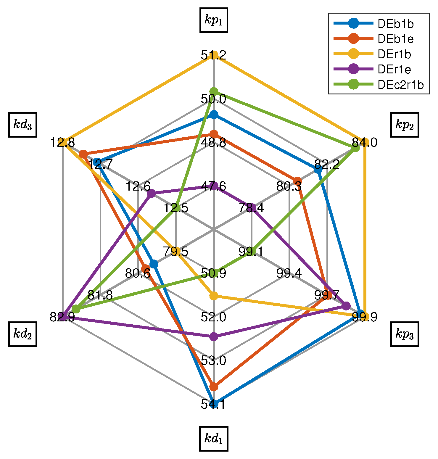
4.2. Statistical Analysis of the Algorithm Performance

This section presents an analysis of the algorithm’s performance to identify the most outstanding differential evolution variants in the controller tuning approach for robot–environment interactions, and hence, to select the most suitable solution.
As a starting point, the mean computation time of each execution is around 3.86 h. It is important to note that this optimization is performed offline, so the computational cost does not impact the system’s real-time performance during operation.
Table 3 presents the descriptive statistical results of the thirty executions of five variants of the DE algorithm. The first column indicates the algorithm variant used in each case. The following columns show the summary statistics obtained. From the second to the fifth column, the results for the best, worst, average, and standard deviation of the thirty executions per algorithm are presented. The best result for each criterion is highlighted in bold. The graphical representation of the descriptive statistics is also presented in Figure 5. To generalize the results obtained, inferential statistics are applied to confirm the performance of the algorithms through a multiple comparison test [56]. Before using the test, it is essential to ensure that at least two samples (sets of thirty executions in the group of five sets provided by each DE variant) have different ranks, i.e., the Friedman test can detect differences between at least two samples. In this particular case, the p-value is 2.79 × 10 14 , indicating the existence of significant differences. So, once this is confirmed, the Bonferroni multiple comparison post hoc test with a significance level α = 0.05 would confirm the algorithm performance among them. The multiple comparison test is shown in Figure 6. Lines overlapping indicate no significant difference between the algorithms; i.e., no inference about the data distributions can be made, as the p-values in those comparisons are larger than the chosen significance level. In contrast, algorithm results that vary significantly from each other do not have overlapping red lines, meaning that the p-value is below the chosen significance level. The winner is the algorithm closest to the left in the rankings (x-axis in the figure). Figure 6 compares one of the most promising algorithms (DE/best/1/bin) with the rest of them. Algorithms different from the DE/best/1/bin are depicted in red lines, whereas gray lines indicate algorithms that are not significantly different.
From the descriptive and inferential statistics, the following findings are stated:
  • The most promising algorithms are DE/best/1/bin and DE/best/1/exp among the DE variants. The inferential statistics indicate no significant difference (as shown by the overlap in the figure) and, thus, those algorithms perform similarly.
  • DE/best/1/bin provides the best value through the particular thirty executions according to the descriptive statistics.
  • The DE/rand/1/bin, DE/rand/1/exp, and DE/current-to-rand/1/bin perform similarly (those overlap in the figure), and those represent the worst algorithms for the particular controller tuning problem.
Table 4 presents the performance function obtained without the stochastic nature of the noise in the controller of the OMR dynamics, considering the controller parameters obtained by different DE variants. The evaluation of ISE is given in the first column, the ISDU in the second column, and the objective function in the third column. The best results obtained in each column are highlighted in bold. It is confirmed that DE/best/1/exp achieves the best overall performance and also the lowest ISE value, while the DE/rand/1/bin only excels in the ISDU. So, the second-best performance is given by DE/best/1/bin. These findings are consistent with the inferential statistics, which indicate that both DE/best variants exhibit the most competitive performance across all crossovers (binomial or exponential).
Finally, the controller gains obtained from the optimization process using the five DE variants are presented in Table 5. The radar plot in Figure 7 provides visual information about the differences or similarities of the obtained gains. As expected, it is observed that the gains found by the DE/best/1/bin and DE/best/1/exp have a similar shape in the radar graph, due to their similar performance, as indicated in the inferential statistics.

4.3. Validation of the Controller Tuning Approach for Robot–Environment Interactions

The validation consists of two stages. In the first part, the simulation results and experimental outcomes are presented to evaluate their performance, confirming the correctness of the proposed Controller Tuning Approach with robot–environment Interactions (CTAwREI). The experimental and simulation tests both take into account the same initial conditions, controller gains, obstacle’s position, and the same parameters for the virtual external force (numerically simulated as a spring-like model). The sampling time of the experimental result is 5 ms. The second part of this section highlights the importance of formulating the proposed controller tuning approach by comparing it with an alternative approach. The third part of this section incorporates a force transducer into the experimental platform to validate the proposal’s robustness using an actual sensing system in the environment.

4.3.1. Simulation–Experimentation Results with Virtual External Force

Figure 8 displays the schematic diagram of the physical testbed platform’s general overview, where the closed-loop system for the real OMR prototype is applied. The prototype features a mini-ITX GA-D425TUD motherboard with an Intel® processor, Atom D525, 4 GB of RAM, and a 250 GB solid-state drive. The control system is programmed in Simulink® R2012a software with the odometry system [57] for OMR’s position. The external force is numerically obtained using a spring-like model, as previously described, and also measured using an SI-130-10 Gamma six-axis force/torque sensor, along with the F/T controller for the signal conditioning system, both manufactured by ATI Industrial Automation (Apex, NC, USA). The force/torque sensor is also implemented in the next section to validate the proposed CTAwREI with an actual sensor. The motor position data acquisition and the sampling signals (along with the control signal) are provided by the Sensoray 626 PCI data acquisition card. Three servo drivers of the Advanced Motion 12A8 series provide the amplification of the control signal to the three OMR’s brushed DC motors. The OMR’s electrical components receive the necessary voltages of 14 V and 30 V from external DC power sources. The physical testbed platform is shown in Figure 9.
The gains obtained by the DE/best/1/bin are considered to perform the simulation and experimentation analysis using the virtual external force. Figure 10 shows the generated trajectory in the Cartesian space, in Figure 11 the control signals are provided, and in Figure 12 the external forces applied to the OMR are displayed. Both simulation and experimental results present suitable behaviors. The observed difference is mainly attributed to unmodeled dynamics, such as friction, OMR velocity estimation, among others.
The reaction forces of the controller due to the collision of the obstacle are presented around the time interval [50, 120] s. The maximum errors between the desired trajectory and the current behavior in simulation and experimentation at the time when the robot collides with the obstacle are 0.6097 m and 0.7931 m for the X w Y w linear displacements in simulation and experimentation, respectively. This error is attributed to the influence distance of the obstacle ( λ 0 = 0.28 ) plus the mobile robot influence distance ( ϵ = 0.287 ). In the same fashion, the angular displacement maximum errors are 0.2037 rad and 1.0419 rad, in simulation and experimentation, respectively. In the part of the trajectory where the robot does not collide, the X w Y w linear displacement maximum errors in simulation and experimentation are 1.49 × 10 4 m and 0.0198 m, respectively. In the same manner, the angular displacement maximum errors are 3.9 × 10 5 rad and 0.0201 rad, respectively. This indicates that once the OMR does not collide with the obstacle, the OMR can follow the desired trajectory efficiently.
It is also observed that the control signals repel the obstacle with the maximum applied torque (±5 Nm) around the time interval [50, 100] s. When this happens, the external force applied to the OMR is below 0.6 N, which is equivalent to moving a small object of 0.06 kg. So, these forces do not affect the safe and comfortable interactions between the environment and the OMR. Once the OMR is free of the obstacle, the control signal allows the desired trajectory to be tracked.

4.3.2. Comparative Results

In this section, the proposed CTAwREI is compared with a controller tuning approach that only considers the ISE performance index. This comparative approach does not consider improving control smoothness, which could reveal whether it is beneficial in situations with interactions. The primary objective of this section is to demonstrate the benefits of utilizing the tradeoff between the ISE and the ISDU in the proposed CTAwREI. The comparative controller tuning approach is named Comparative Controller Tuning Approach (CCTA) and is formulated as in (14)–(16), with the difference that the performance function consists of only one term (ISE). The optimization problem of CCTA is solved using one of the two most outstanding DE variants in this case study, i.e., using DE/best/1/exp. The obtained gains are given as follows: k p 1 = 52.17238 , k p 2 = 79.76143 , k p 3 = 99.79305 , k d 1 = 55.42128 , k d 2 = 89.82195 , and k d 3 = 15.02795 .
Figure 13 represents the behavior of the OMR with the controller gains obtained via CCTA. The control signal is also presented in Figure 14. The applied external force to the OMR with the controller gains obtained via CCTA is displayed in Figure 15. Table 6 shows the numerical comparative analysis of the proposed CTAwREI concerning the CCTA in Simulation (Sim) and Experimentation (Exp). The table presents the values of the Root Mean Square (RMS) of the external resultant force in the third column, as well as the the Maximum Error Distance without Obstacle (MEDwO), the ISE, the ISDU, and the performance function J within the following columns. The MEDwO is the maximum error distance between the desired trajectory and the OMR trajectory when the robot does not collide with the obstacle, i.e., in the time interval [ 0 , 50 ] [ 120 , 210 ] s . The following findings are given:
  • The tradeoff between the tracking error and the controller signal’s smoothness is an important factor to be considered in the robot–environment interaction task. It is observed that the proposed CTAwREI reduces the tradeoff related to the performance function J by 61.57 % in simulations concerning the CCTA (see J column). The experimental results reveal a reduction of 2.08 % in such a tradeoff.
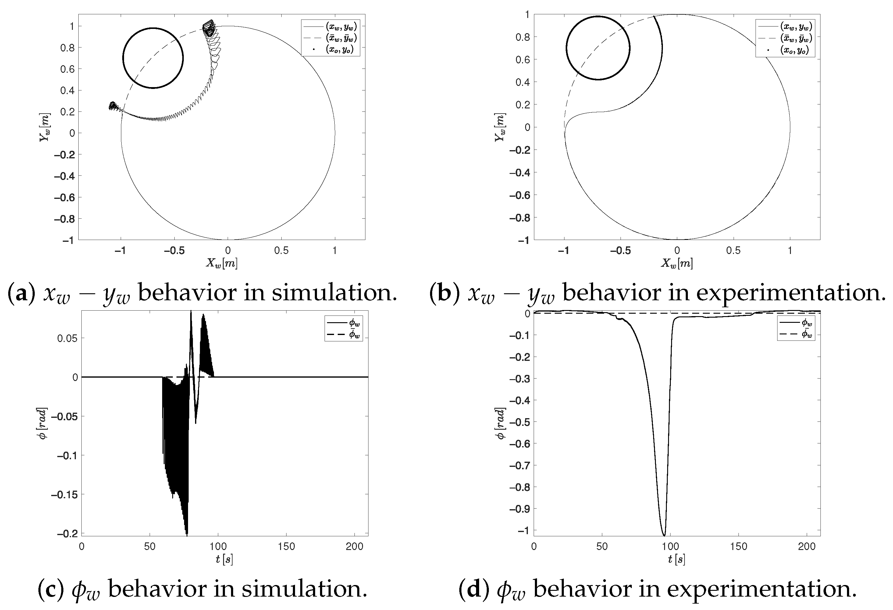
  • Once the OMR moves beyond the obstacle, the proposed CTAwREI reduces the tracking error in the Cartesian position and orientation compared to CCTA by 98.76 % and 90.1763 % , respectively. In the experimental results, the tracking reduction is around 1.47 % and 1.49 % , respectively. Those results can be visualized in the MEDwO column of Table 6. In Figure 10a,b and Figure 13a,b, these errors are also observed in the segments where the presence of the obstacle does not influence the OMR.
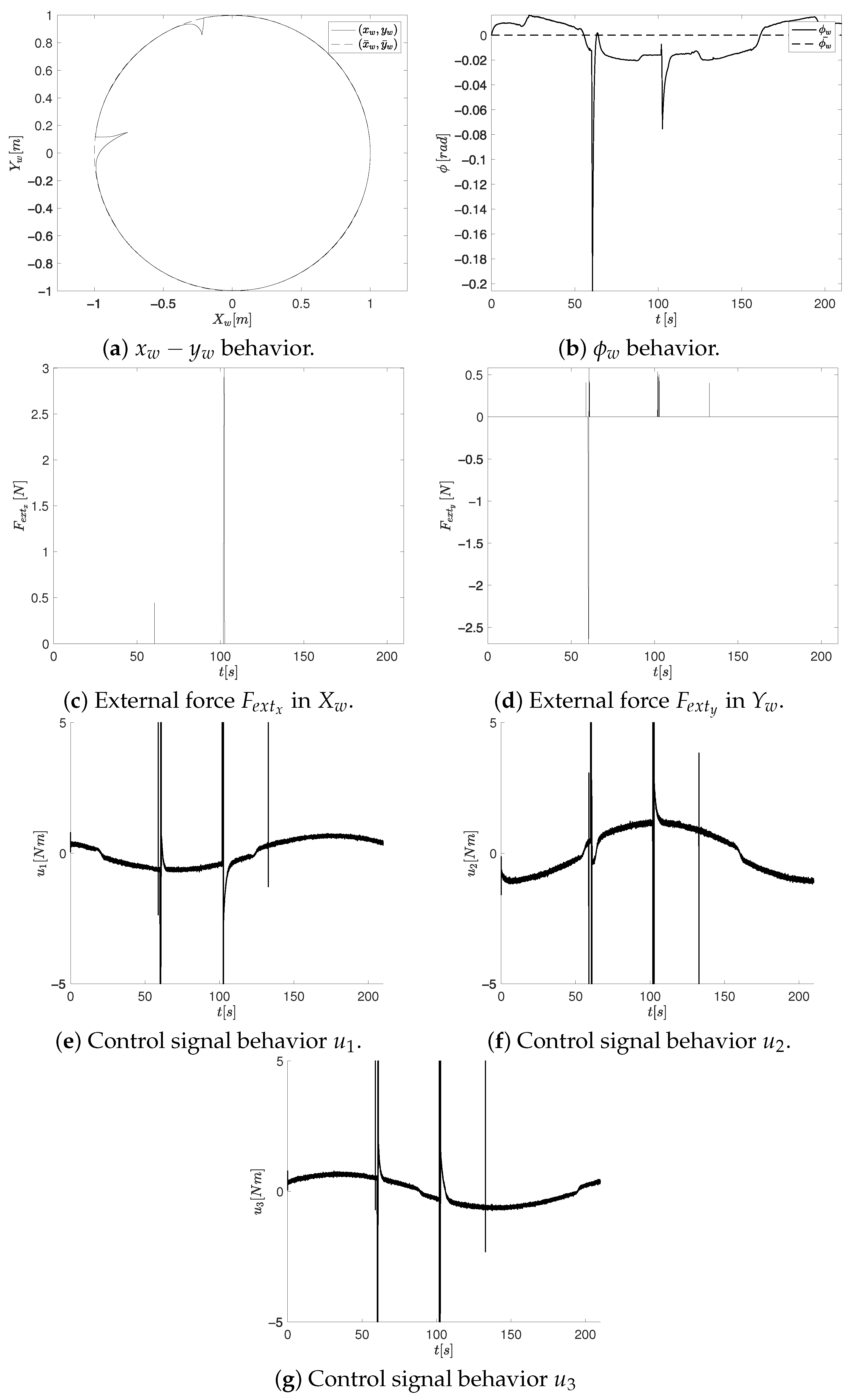
  • The control signals of the proposal in the simulation are significantly smoother than the CCTA, as indicated in the ISDU column of Table 6 with a reduction of 99.23 % . This is also visualized in Figure 14, where the control signals commute between their limits. The lack of control smoothness in the controller tuning formulation of the comparative controller tuning approach could have an impact on the high vibration of the OMR and an increase in energy consumption. In the case of the experimental result, the reduction of the control signal is 2.77 % .
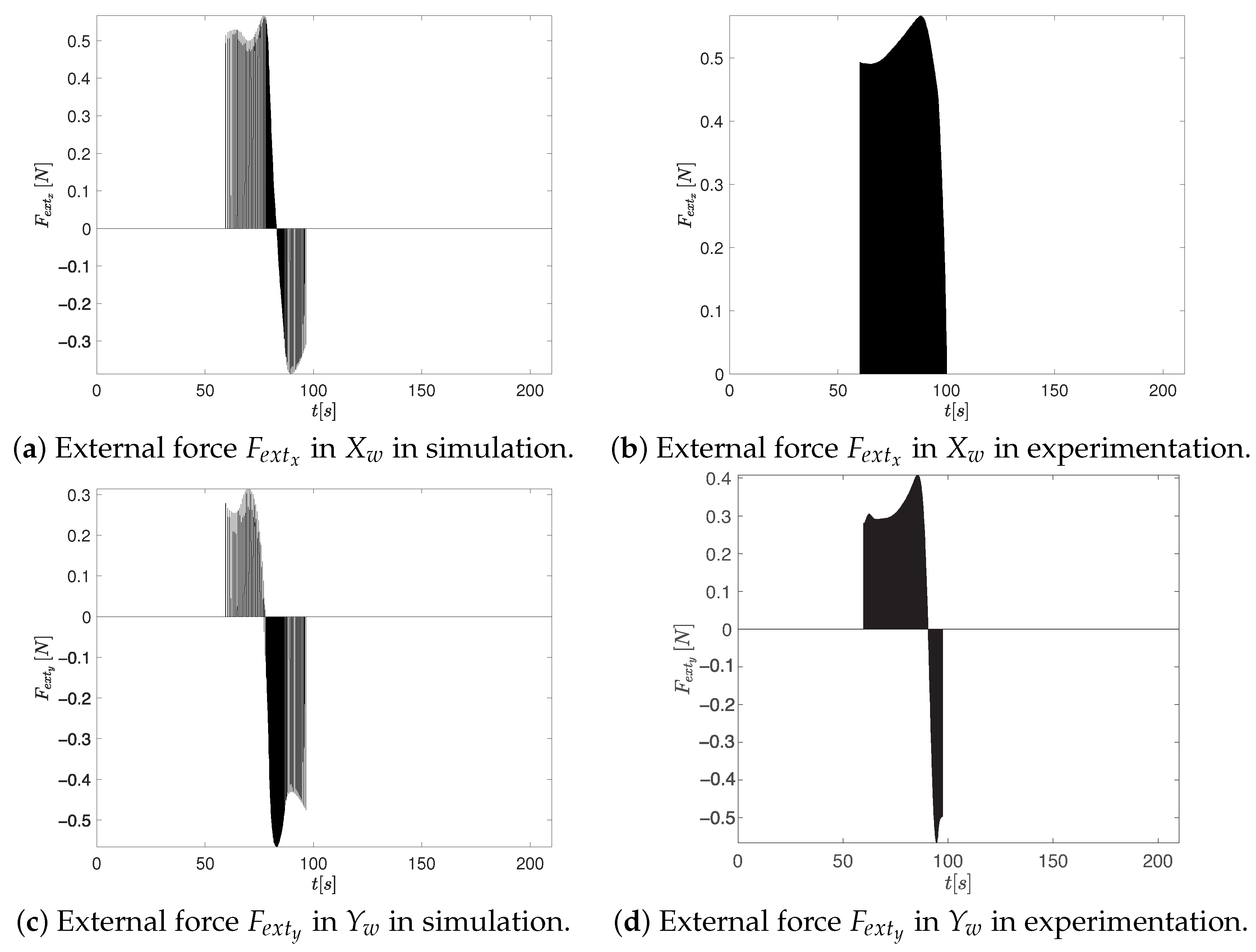
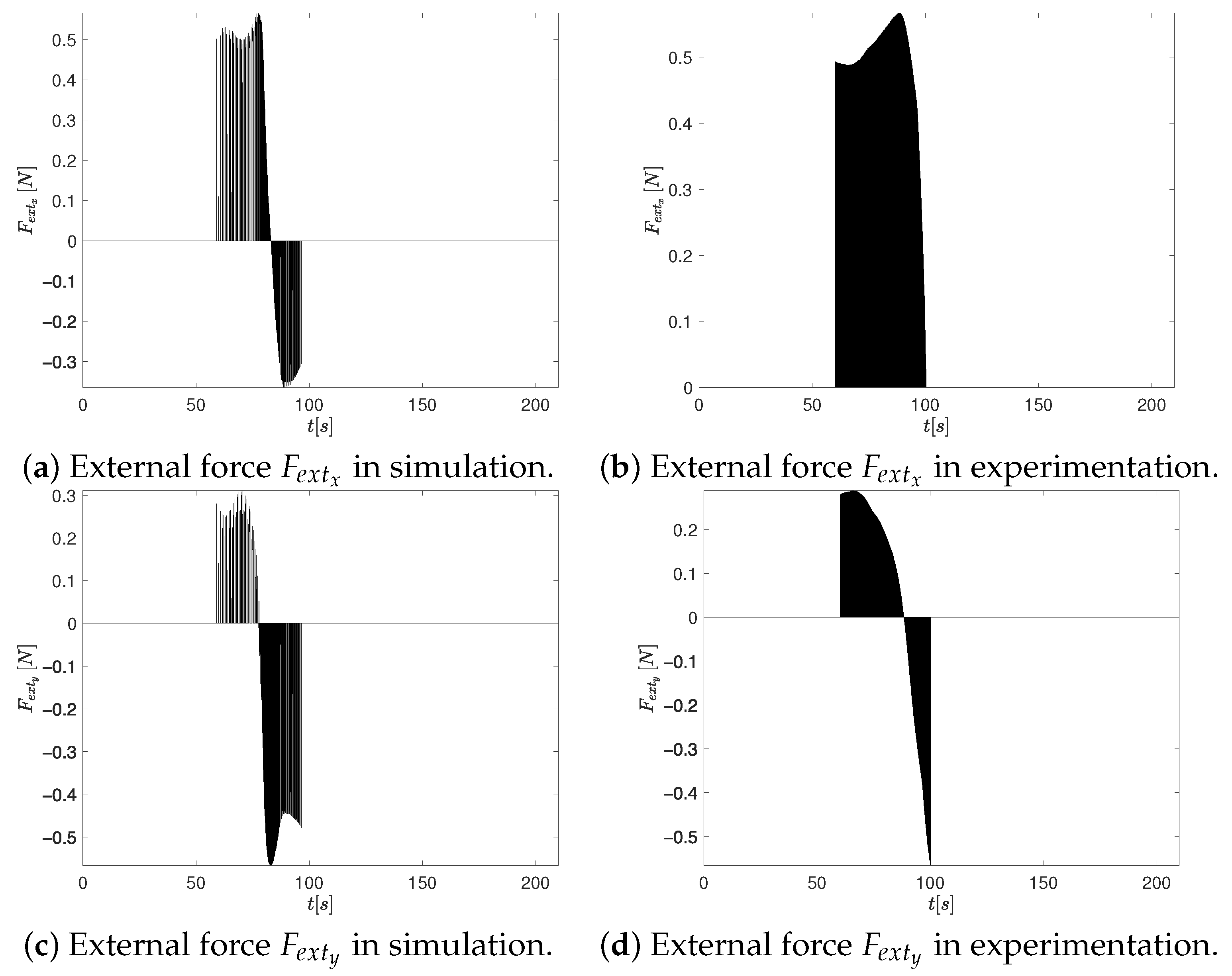
  • Although both controller tuning approaches exhibit similar overall behavior in terms of external forces (see Figure 12 and Figure 15), a noticeable difference arises in the Y w axis force component F e x t y during experimentation. Specifically, the CTAwREI approach produces a slightly higher peak in F e x t y of 0.4 N compared to 0.3 N in the CCTA approach. This increase can be attributed to a redistribution of the repulsive force components along the X w and Y w directions, resulting from the interaction between the repulsive potential field and the optimized controller gains. While F e x t y increases, a compensatory reduction in F e x t x is observed, indicating that the overall external interaction force is not intensified but rather reoriented. It is important to note that the resultant external force is determined by both components, F e x t x and F e x t y . Despite the higher peak in F e x t y , the RMS value of the resultant external force in CTAwREI is 0.09 % lower than in CCTA (see the experimentation in column RMS ρ ( F e x t ) of Table 6). It is important to note that the RMS value of the resultant external force in CTAwREI is also reduced by 1.45 % in the simulation. This marginal reduction suggests a more balanced force distribution, which contributes to smoother control actions, enhanced stability during interaction, and potentially lower energy consumption.
  • In a real-world scenario, the proposed approach, which incorporates the synergy between the tracking error and the controller signal smoothness, benefits from the fact that once disturbed by an obstacle, the robot can follow the path more precisely and smoothly (see the MEDwO column), positively affecting energy consumption. Despite the fact that the experimental improvements are smaller compared to those observed in simulation, in practice, even slight improvements observed in experimental testing can significantly impact the task execution, particularly in high-precision applications where even minimal deviations can lead to significant performance degradation.

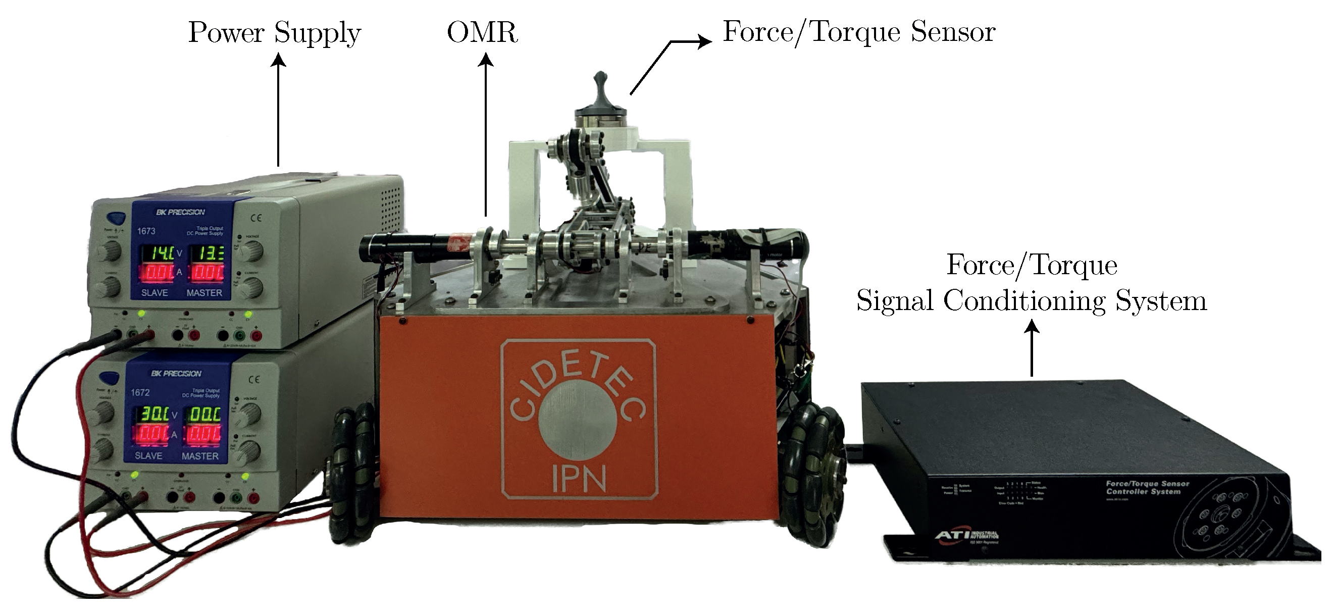
4.3.3. Experimentation Results with an Actual Force System

In this section, the proposed CTEwREI is validated using an actual force system in place of the virtual sensor. This additional experiment corroborates the CTEwREI performance with other external force behaviors and shows if the obtained gains are also suitable for robot–environment interactions. The external force is provided in the mass center of the OMR, as is observed in Figure 9.
Under the same CTEwREI gains, trajectory, and sample time, the additional experiment involves applying external disturbances at two distinct time instants. Figure 16 displays the OMR’s position behavior, the control signal, and the external force.
The first time that the external force is applied to the sensor is within the interval [ 60.11 , 60.73 ] (s). During this interval, the measured external force presents maximum absolute values of 0.444 (N) and 2.6935 (N) for the force components ( F e x t x and F e x t y ), respectively. The measured RMS of the resultant force vector is 1.6719 (N) with an average orientation of 1.2460 (rad). Another external force is exerted at the interval [ 101.79 , 102.58 ] (s). The maximum absolute values of the F e x t x and F e x t y components during this interval are 3.0024 (N) and 0.5354 (N) with a reported RMS of the resultant force vector of 2.2013 (N) with an average orientation of 0.0708 (rad). Notably, the three control signals u 1 , u 2 , and u 3 present smooth behavior during the OMR operation, exhibiting abrupt changes only when an external force is sensed. It is also observed that within a short time interval of approximately 132 s, the sensor system detected a force disturbance caused by vibrations generated by the rollers of the OMR’s wheels, which affected the control signals. However, the overall behavior of OMR remains unaffected. This latest result demonstrates that the proposed Controller Tuning Approach with robot–environment Interactions is functional for a real robot–environment interaction application utilizing an actual force sensor.

5. Conclusions

This work presents a controller tuning approach with robot–environment interactions (CTAwREI) based on differential evolution optimizers, where the tradeoff between the trajectory tracking error and control effort fluctuations is considered to maintain the controller performance in an environment with obstacles. The robot–environment interaction is incorporated into the controller through repulsive forces from virtual potential fields, where a spring-like model effectively simulates the influence of obstacles.
The controller’s stability analysis reveals a strong relationship between the repulsive force and the controller gains, which is crucial for controller stabilization. Consequently, the proposed controller tuning approach effectively ensures stable behavior in environments with obstacles.
The proposal was applied to a (3,0) mobile robot in numerical simulations and experimentation with a physical testbed platform that replicates virtual interaction scenarios. The inferential statistic through a multiple comparison test confirms with a 95 % of confidence that among the most promising DE variants (DE/rand/1/bin, DE/rand/1/exp, DE/best/1/bin, DE/best/1/exp, and DE/current-to-rand/1/bin), the DE/best variants (DE/best/1/bin and DE/best/1/exp) outperform the rest of the optimizers.
The proposed CTAwREI’s comparative results with the CCTA indicate that both present effective interaction with virtual obstacles, exerting a minimum external force, but in the former case, with the best tradeoff between trajectory tracking error and control effort fluctuations. This improvement in the synergy of the performance function terms led to a substantial average reduction in the trajectory tracking error: 94.46 % in simulation and a consistent 1.48 % in experimentation, along the path unaffected by the presence of obstacles, compared to CCTA. Notably, the experimental result confirms the practical effectiveness of the proposed tuning approach under real-world conditions. Furthermore, regarding control signal smoothness, the proposed method achieved a remarkable reduction of 99.23 % in simulation and 2.77 % in experimentation. Although the improvement observed in the experimental tests for the particular case study is smaller in magnitude than the simulations, it is still noteworthy, particularly in high-precision applications where even minimal deviations can lead to significant performance degradation.
The experimental tests also validate the controller’s tuning ability to maintain performance under the uncertainties inherent in real-world conditions, including sensor noise, and unmodeled dynamics. This validation is crucial, as even relatively small experimental improvements often represent significant practical enhancements when transferring control strategies from ideal simulations to physical platforms.
The CTEwREI’s adaptability is also validated with an actual force system instead of a virtual external force, which confirms its applicability to real external force behavior. Unlike the techniques described to date, our approach is not only effective in simulation environments but also demonstrates reliable performance in real-world applications using actual force sensors. This highlights its potential as a practical and reliable solution for tuning the robot–environment interaction controller in omnidirectional mobile robotic systems.
The proposed approach is evaluated on a specific (3,0) mobile robot, but can be extended to other robotic systems. Future work will involve testing the proposal for a broader range of robotic systems.
On the other hand, even though results obtained in simulation and experiments confirm the effectiveness of the proposed approach, certain limitations may affect control accuracy, especially in position, velocity, and force estimates. Although Gaussian noise is included in the simulations to approximate these conditions, in real-life environments, this noise can be more complex in specific applications. Nonetheless, the proposal does not explicitly consider unmodeled dynamics that may alter the expected behavior, especially when high precision is required or conditions change rapidly. Another future work is related to the integration of observers and adaptive models into the offline controller tuning approach to address these challenges. In this direction, adaptive disturbance observer-based fixed-time control methods offer promising tools to enhance robustness and disturbance rejection under uncertain conditions [58].

Author Contributions

J.A.P.-B.: Validation, Conceptualization, Formal analysis, Investigation, Visualization, Methodology, Writing—original draft preparation, Writing—review and editing, Software. M.G.V.-C.: Methodology, Conceptualization, Investigation, Writing—original draft preparation, Writing—review and editing, Resources, Supervision, Project administration, Funding acquisition. S.E.B.-G.: Conceptualization, Methodology, Resources, Investigation. A.R.-M.: Investigation, Visualization, Writing—original draft preparation, Writing—review and editing. A.G.R.-L.: Investigation, Data curation, Software, Validation, Writing—original draft preparation. V.M.S.-G.: Conceptualization, Resources, Validation. All authors have read and agreed to the published version of the manuscript.

Funding

This work was supported by the Secretaría de Investigación y Posgrado (SIP) of the Instituto Politécnico Nacional [grant numbers 20241335, 20250216].

Data Availability Statement

Data will be made available on request.

Conflicts of Interest

The authors declare no conflicts of interest.

References

  1. Zhu, J.; Lyu, L.; Xu, Y.; Liang, H.; Zhang, X.; Ding, H.; Wu, Z. Intelligent soft surgical robots for next-generation minimally invasive surgery. Adv. Intell. Syst. 2021, 3, 2100011. [Google Scholar] [CrossRef]
  2. Yang, L.; Zhang, Z.; Zhang, Z.; Lou, Y.; Han, S.; Liu, J.; Fang, L.; Zhang, S. Design of Heavy-Load Soft Robots Based on a Dual Biomimetic Structure. Biomimetics 2024, 9, 398. [Google Scholar] [CrossRef] [PubMed]
  3. Pan, L. Motion trajectory control system for production line robots based on variable domain fuzzy control. Adv. Multimed. 2022, 2022, 3893937. [Google Scholar] [CrossRef]
  4. Spong, M.W. Robot Dynamics and Control, 1st ed.; John Wiley & Sons, Inc.: Hoboken, NJ, USA, 1989. [Google Scholar]
  5. Ogata, K. Modern Control Engineering, 4th ed.; Prentice Hall PTR: Hoboken, NJ, USA, 2001. [Google Scholar]
  6. Borase, R.P.; Maghade, D.; Sondkar, S.; Pawar, S. A review of PID control, tuning methods and applications. Int. J. Dyn. Control 2021, 9, 818–827. [Google Scholar] [CrossRef]
  7. Rodríguez-Molina, A.; Mezura-Montes, E.; Villarreal-Cervantes, M.G.; Aldape-Pérez, M. Multi-objective meta-heuristic optimization in intelligent control: A survey on the controller tuning problem. Appl. Soft Comput. 2020, 93, 106342. [Google Scholar] [CrossRef]
  8. Reeves, C.R. Heuristic search methods: A review. In Operational Research-Keynote Papers; Springer: Cham, Switzerland, 1996; pp. 122–149. [Google Scholar]
  9. Franceschi, P.; Castaman, N.; Ghidoni, S.; Pedrocchi, N. Precise Robotic Manipulation of Bulky Components. IEEE Access 2020, 8, 222476–222485. [Google Scholar] [CrossRef]
  10. Vignesh, C.; Uma, M.; Sethuramalingam, P. Development of rapidly exploring random tree based autonomous mobile robot navigation and velocity predictions using K-nearest neighbors with fuzzy logic analysis. Int. J. Interact. Des. Manuf. (IJIDeM) 2024, 18, 1–25. [Google Scholar] [CrossRef]
  11. Zhou, Q.; Feng, H.; Liu, Y. Multigene and Improved Anti-Collision RRT* Algorithms for Unmanned Aerial Vehicle Task Allocation and Route Planning in an Urban Air Mobility Scenario. Biomimetics 2024, 9, 125. [Google Scholar] [CrossRef]
  12. Sun, X.; Deng, S.; Tong, B.; Wang, S.; Zhang, C.; Jiang, Y. Hierarchical framework for mobile robots to effectively and autonomously explore unknown environments. ISA Trans. 2023, 134, 1–15. [Google Scholar] [CrossRef]
  13. Sharma, U.; Medasetti, U.S.; Deemyad, T.; Mashal, M.; Yadav, V. Mobile Robot for Security Applications in Remotely Operated Advanced Reactors. Appl. Sci. 2024, 14, 2552. [Google Scholar] [CrossRef]
  14. Taheri, H.; Zhao, C.X. Omnidirectional mobile robots, mechanisms and navigation approaches. Mech. Mach. Theory 2020, 153, 103958. [Google Scholar] [CrossRef]
  15. Achirei, S.D.; Mocanu, R.; Popovici, A.T.; Dosoftei, C.C. Model-predictive control for omnidirectional mobile robots in logistic environments based on object detection using CNNs. Sensors 2023, 23, 4992. [Google Scholar] [CrossRef] [PubMed]
  16. Tao, Y.; Li, M.; Cao, X.; Lu, P. Mobile robot collision avoidance based on deep reinforcement learning with motion constraints. IEEE Trans. Intell. Veh. 2024. [Google Scholar] [CrossRef]
  17. Mirsky, R.; Xiao, X.; Hart, J.; Stone, P. Conflict Avoidance in Social Navigation—A Survey. ACM Trans. Hum.-Robot. Interact. 2024, 13, 1–36. [Google Scholar] [CrossRef]
  18. Spiess, F.; Reinhart, L.; Strobel, N.; Kaiser, D.; Kounev, S.; Kaupp, T. People detection with depth silhouettes and convolutional neural networks on a mobile robot. J. Image Graph. 2021, 9, 135–139. [Google Scholar] [CrossRef]
  19. Zhang, J.; Lu, Y.; Che, L.; Zhou, M. Moving-distance-minimized PSO for mobile robot swarm. IEEE Trans. Cybern. 2021, 52, 9871–9881. [Google Scholar] [CrossRef]
  20. Rodriguez-Molina, A.; Solis-Romero, J.; Villarreal-Cervantes, M.G.; Serrano-Perez, O.; Flores-Caballero, G. Path-planning for mobile robots using a novel variable-length differential evolution variant. Mathematics 2021, 9, 357. [Google Scholar] [CrossRef]
  21. da Rocha Balthazar, G.; Silveira, R.M.F.; da Silva, I.J.O. How Do Escape Distance Behavior of Broiler Chickens Change in Response to a Mobile Robot Moving at Two Different Speeds? Animals 2024, 14, 1014. [Google Scholar] [CrossRef]
  22. Villani, L.; De Schutter, J. Force Control. In Springer Handbook of Robotics; Springer: Berlin/Heidelberg, Germany, 2016; pp. 195–220. [Google Scholar]
  23. Shin, H.; Kim, S.; Seo, K.; Rhim, S. A virtual pressure and force sensor for safety evaluation in collaboration robot application. Sensors 2019, 19, 4328. [Google Scholar] [CrossRef]
  24. Sharkawy, A.N.; Ma’arif, A.; Furizal; Sekhar, R.; Shah, P. A Comprehensive Pattern Recognition Neural Network for Collision Classification Using Force Sensor Signals. Robotics 2023, 12, 124. [Google Scholar] [CrossRef]
  25. Li, S.; Xu, J. Multiaxis Force/Torque Sensor Technologies: Design Principles and Robotic Force Control Applications: A Review. IEEE Sens. J. 2025, 25, 4055–4069. [Google Scholar] [CrossRef]
  26. Park, K.M.; Park, F.C. Collision Detection for Robot Manipulators: Methods and Algorithms; Springer: Berlin/Heidelberg, Germany, 2023. [Google Scholar]
  27. Yousefizadeh, S.; Bak, T. Unknown external force estimation and collision detection for a cooperative robot. Robotica 2020, 38, 1665–1681. [Google Scholar] [CrossRef]
  28. Liu, S.; Wang, L.; Wang, X.V. Sensorless force estimation for industrial robots using disturbance observer and neural learning of friction approximation. Robot. Comput.-Integr. Manuf. 2021, 71, 102168. [Google Scholar] [CrossRef]
  29. Zurlo, D.; Heitmann, T.; Morlock, M.; De Luca, A. Collision Detection and Contact Point Estimation Using Virtual Joint Torque Sensing Applied to a Cobot. In Proceedings of the 2023 IEEE International Conference on Robotics and Automation (ICRA), London, UK, 29 May–2 June 2023; pp. 7533–7539. [Google Scholar] [CrossRef]
  30. Rosales, A.; Heikkilä, T. Analysis and design of direct force control for robots in contact with uneven surfaces. Appl. Sci. 2023, 13, 7233. [Google Scholar] [CrossRef]
  31. Abbas, M.; Al Issa, S.; Dwivedy, S.K. Event-triggered adaptive hybrid position-force control for robot-assisted ultrasonic examination system. J. Intell. Robot. Syst. 2021, 102, 84. [Google Scholar] [CrossRef]
  32. Zhou, B.; Song, F.; Liu, Y.; Fang, F.; Gan, Y. Robust sliding mode impedance control of manipulators for complex force-controlled operations. Nonlinear Dyn. 2023, 111, 22267–22281. [Google Scholar] [CrossRef]
  33. Yoon, I.; Na, M.; Song, J.B. Assembly of low-stiffness parts through admittance control with adaptive stiffness. Robot. Comput.-Integr. Manuf. 2024, 86, 102678. [Google Scholar] [CrossRef]
  34. Tao, Q.; Liu, J.; Zheng, Y.; Yang, Y.; Lin, C.; Guang, C. Evaluation of an active disturbance rejection controller for ophthalmic robots with piezo-driven injector. Micromachines 2024, 15, 833. [Google Scholar] [CrossRef]
  35. Roveda, L.; Piga, D. Sensorless environment stiffness and interaction force estimation for impedance control tuning in robotized interaction tasks. Auton. Robot. 2021, 45, 371–388. [Google Scholar] [CrossRef]
  36. Abdullah Hashim, A.A.; Ghani, N.M.A.; Tokhi, M.O. Enhanced PID for pedal vehicle force control using hybrid spiral sine-cosine optimization and experimental validation. J. Low Freq. Noise Vib. Act. Control. 2025, 14613484251320723. [Google Scholar] [CrossRef]
  37. Chen, J.; Deng, L.; Hua, Z.; Ying, W.; Zhao, J. Bayesian optimization-based efficient impedance controller tuning for robotic interaction with force feedback. IEEE Trans. Instrum. Meas. 2023, 72, 1–10. [Google Scholar] [CrossRef]
  38. Yanyong, S.; Kaitwanidvilai, S. Experimental realization of PSO-based hybrid adaptive sliding mode control for force impedance control systems. Results Control. Optim. 2025, 19, 100548. [Google Scholar] [CrossRef]
  39. Zhai, J.; Zeng, X.; Su, Z. An intelligent control system for robot massaging with uncertain skin characteristics. Ind. Robot. Int. J. Robot. Res. Appl. 2022, 49, 634–644. [Google Scholar] [CrossRef]
  40. Shaw, J.S.; Lee, S.Y. Using genetic algorithm for drawing path planning in a robotic arm pencil sketching system. Proc. Inst. Mech. Eng. Part C J. Mech. Eng. Sci. 2024, 238, 7134–7142. [Google Scholar] [CrossRef]
  41. Sun, C.; Zhu, H. Active Disturbance Rejection Control of Bearingless Permanent Magnet Slice Motor Based on RPROP Neural Network Optimized by Improved Differential Evolution Algorithm. IEEE Trans. Power Electron. 2024, 39, 3064–3074. [Google Scholar] [CrossRef]
  42. Ahmed, H.; As’arry, A.; Hairuddin, A.A.; Khair Hassan, M.; Liu, Y.; Onwudinjo, E.C.U. Online DE Optimization for Fuzzy-PID Controller of Semi-Active Suspension System Featuring MR Damper. IEEE Access 2022, 10, 129125–129138. [Google Scholar] [CrossRef]
  43. Meng, M.; Zhou, C.; Lv, Z.; Zheng, L.; Feng, W.; Wu, T.; Zhang, X. Research on a Method of Robot Grinding Force Tracking and Compensation Based on Deep Genetic Algorithm. Machines 2023, 11, 1075. [Google Scholar] [CrossRef]
  44. Storn, R.; Price, K. Differential Evolution—A Simple and Efficient Heuristic for global Optimization over Continuous Spaces. J. Glob. Optim. 1997, 11, 341–359. [Google Scholar] [CrossRef]
  45. Serrano-Pérez, O.; Villarreal-Cervantes, M.G.; Rodríguez-Molina, A.; Serrano-Pérez, J. Offline robust tuning of the motion control for omnidirectional mobile robots. Appl. Soft Comput. 2021, 110, 107648. [Google Scholar] [CrossRef]
  46. Mousakazemi, S.M.H. Comparison of the error-integral performance indexes in a GA-tuned PID controlling system of a PWR-type nuclear reactor point-kinetics model. Prog. Nucl. Energy 2021, 132, 103604. [Google Scholar] [CrossRef]
  47. Tavazoei, M.S. Notes on integral performance indices in fractional-order control systems. J. Process. Control. 2010, 20, 285–291. [Google Scholar] [CrossRef]
  48. Reynoso-Meza, G.; Garcia-Nieto, S.; Sanchis, J.; Blasco, F.X. Controller Tuning by Means of Multi-Objective Optimization Algorithms: A Global Tuning Framework. IEEE Trans. Control. Syst. Technol. 2013, 21, 445–458. [Google Scholar] [CrossRef]
  49. Osyczka, A. Multicriterion Optimization in Engineering with FORTRAN Programs; Ellis Horwood Series in Engineering Science; E. Horwood: Chichester, UK, 1984. [Google Scholar]
  50. Villarreal-Cervantes, M.G.; Cruz-Villar, C.A.; Álvarez-Gallegos, J.; Portilla-Flores, E.A. Kinematic dexterity maximization of an omnidirectional wheeled mobile robot: A comparison of metaheuristic and sqp algorithms. Int. J. Adv. Robot. Syst. 2012, 9, 161. [Google Scholar] [CrossRef]
  51. Vázquez, J.; Velasco-Villa, M. Path-Tracking Dynamic Model Based Control of an Omnidirectional Mobile Robot. IFAC Proc. Vol. 2008, 41, 5365–5370. [Google Scholar] [CrossRef]
  52. Villarreal-Cervantes, M.G.; Alvarez-Gallegos, J. Off-line PID control tuning for a planar parallel robot using DE variants. Expert Syst. Appl. 2016, 64, 444–454. [Google Scholar] [CrossRef]
  53. Rojas-López, A.G.; Villarreal-Cervantes, M.G.; Rodríguez-Molina, A. Optimum Online Controller Tuning Through DE and PSO Algorithms: Comparative Study with BLDC Motor and Offline Controller Tuning Strategy. In Proceedings of the 2023 10th International Conference on Soft Computing & Machine Intelligence (ISCMI), Mexico City, Mexico, 25–26 November 2023; pp. 215–221. [Google Scholar] [CrossRef]
  54. Serrano-Pérez, O.; Villarreal-Cervantes, M.G.; González-Robles, J.C.; Rodríguez-Molina, A. Meta-heuristic algorithms for the control tuning of omnidirectional mobile robots. Eng. Optim. 2020, 52, 325–342. [Google Scholar] [CrossRef]
  55. Huang, C.; Li, Y.; Yao, X. A Survey of Automatic Parameter Tuning Methods for Metaheuristics. IEEE Trans. Evol. Comput. 2020, 24, 201–216. [Google Scholar] [CrossRef]
  56. Derrac, J.; García, S.; Molina, D.; Herrera, F. A practical tutorial on the use of nonparametric statistical tests as a methodology for comparing evolutionary and swarm intelligence algorithms. SWarm Evol. Comput. 2011, 1, 3–18. [Google Scholar] [CrossRef]
  57. Villarreal-Cervantes, M.G.; Guerrero-Castellanos, J.F.; Ramírez-Martínez, S.; Sánchez-Santana, J.P. Stabilization of a (3,0) mobile robot by means of an event-triggered control. ISA Trans. 2015, 58, 605–613. [Google Scholar] [CrossRef]
  58. Liu, Z.; Liu, J.; Zhang, O.; Zhao, Y.; Chen, W.; Gao, Y. Adaptive Disturbance Observer-Based Fixed-Time Tracking Control for Uncertain Robotic Systems. IEEE Trans. Ind. Electron. 2024, 71, 14823–14831. [Google Scholar] [CrossRef]
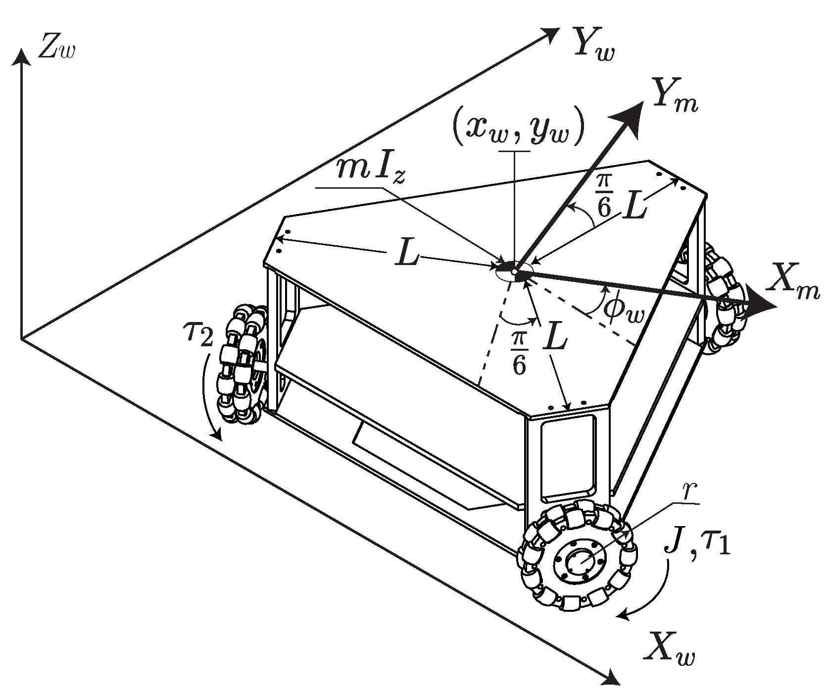
Figure 1. Schematic diagram of the closed-loop system with the external force F r e p .
Mathematics 13 01789 g001
Figure 2. Schematic diagram of the obstacle and the robot.
Mathematics 13 01789 g002
Figure 3. Schematic representation of the OMR in isometric view.
Mathematics 13 01789 g003
Figure 4. Tradeoffs identified through the sensitivity analysis in the weight variations applied in the performance function terms.
Mathematics 13 01789 g004
Figure 5. Box plot of thirty executions for each DE variant (*). The acronyms in the graph represent the following: DEb1b: DE/best/1/bin, DEb1e: DE/best/1/exp, DEr1b: DE/rand/1/bin, DEr1e: DE/rand/1/exp, DEc2r1b: DE/current-to-rand/1/bin.
Mathematics 13 01789 g005
Figure 6. The Bonferroni multiple comparison post hoc test with a significance level of α = 0.05 .
Mathematics 13 01789 g006
Figure 7. Radar plot of the controller gains obtained with the five DE variants.
Mathematics 13 01789 g007
Figure 8. Schematic diagram of the experimental platform for the test of the OMR’s closed-loop system.
Mathematics 13 01789 g008
Figure 9. Testbed platform of the omnidirectional mobile robot (OMR) equipped with a force sensor system for testing robot–environment interaction.
Mathematics 13 01789 g009
Figure 10. Simulation and experimental behavior of the Cartesian position and orientation of the OMR with the best controller gains obtained via best/1/bin in the CTAwREI.
Mathematics 13 01789 g010
Figure 11. Simulation and experimental behavior of the control signal of the OMR with the best controller gains obtained via best/1/bin in the CTAwREI.
Mathematics 13 01789 g011
Figure 12. Simulation and experimental behavior of the external force exerted on the OMR using the best controller gains obtained via best/1/bin in the CTAwREI.
Mathematics 13 01789 g012
Figure 13. Behavior of the Cartesian’s position and orientation of the OMR with the controller gains obtained by the CCTA.
Mathematics 13 01789 g013
Figure 14. Simulation and experimental behavior of the control signal of the OMR with the controller gains obtained via CCTA.
Mathematics 13 01789 g014
Figure 15. Simulation and experimental behavior of the external force exerted on the OMR using the controller gains obtained via CCTA.
Mathematics 13 01789 g015
Figure 16. Experimental behavior of the Cartesian position and orientation, external force, and control signals of the OMR using actual force system.
Mathematics 13 01789 g016
Table 1. Robot parameters.
ParametersDescriptionValueUnits
rWheel radius 0.0625 m
LDistance from the center of mass to the wheel 0.287 m
mMass of the mobile robot 16.319 kg
JWheel inertia 5.82 × 10 4 kgm
I z Inertia of the mobile robot 0.5160 kgm
Table 3. Descriptive statistical result of the thirty executions of the DE variants. The best result for each criterion is highlighted in bold.
DE VariantBestWorstAverageStd. Dev.
DE/best/1/bin0.000174620.000175050.00017489 7.03411 × 10 8
DE/best/1/exp0.000174630.000175070.00017488 6.93427 × 10 8
DE/rand/1/bin0.000174730.00017520.00017504 8.26040 × 10 8
DE/rand/1/exp0.000174740.000175170.00017502 6.80423 × 10 8
DE/current-to-rand/1/bin0.000174730.000175150.00017501 7.60241 × 10 8
Table 4. Used metrics for the results of the closed-loop system performance without random noise. The best result for each criterion is highlighted in bold.
DE VariantISEISDUJ
DE/best/1/bin0.02359570.49879730.0001751
DE/best/1/exp0.02358130.50298120.0001750
DE/rand/1/bin0.02366690.44764110.0001754
DE/rand/1/exp0.02360200.52846440.0001753
DE/current-to-rand/1/bin0.02361050.48711720.0001752
Table 5. Controller gains obtained with the use of DE variants. The best result for each criterion is highlighted in bold.
DE Variant k p 1 k p 2 k p 3 k d 1 k d 2 k d 3
DE/best/1/bin49.5778681.7238999.8780454.0525080.1662912.69077
DE/best/1/exp49.0415480.7065399.6545053.6444780.4155512.72143
DE/rand/1/bin51.2116784.0464799.9099451.4719279.4991112.76682
DE/rand/1/exp47.6271078.4335799.7812052.4464982.9128112.57076
DE/current-to-rand/1/bin50.2074883.5706499.13062450.9273182.5113712.51611
Table 6. Evaluated metrics in the controller tuning approaches.
Controller Tuning ApproachSim/Exp ρ ( F ext ) RMSMEDwO X w Y w / ϕ w ISEISDUJ
CTAwREISim0.1240530.000149/0.0000390.02360.50760.00017
CCTASim0.1258820.012025/0.0003970.023366.7210.00045
CTAwREIExp0.1597260.019885/0.0190220.06431.55260.00047
CCTAExp0.1598700.020182/0.0201230.06461.59690.00048
Disclaimer/Publisher’s Note: The statements, opinions and data contained in all publications are solely those of the individual author(s) and contributor(s) and not of MDPI and/or the editor(s). MDPI and/or the editor(s) disclaim responsibility for any injury to people or property resulting from any ideas, methods, instructions or products referred to in the content.

