Power System Portfolio Selection and CO₂ Emission Management Under Uncertainty Driven by a DNN-Based Stochastic Model

Abstract

A model is proposed to investigate the effects of power generation source diversification and CO₂ emission control in the presence of dispatchable fossil fuel sources and non-dispatchable carbon-free renewables. In a stochastic environment in which three random factors are considered, namely fossil fuels (gas and coal) and CO₂ prices, we discuss a planning methodology for power system portfolio selection that integrates the non-dispatchable renewables available in a given energy system and optimally combines cost, risk and CO₂ emissions. By combining the deep neural network probabilistic forecasting of fossil fuel path prices with a geometric Brownian motion model for describing the CO₂ price dynamics, we simulate a wide range of plausible market scenarios. Results show that under CO₂ price volatility, optimal portfolios shift toward cleaner energy sources, even in the absence of explicit emission targets, highlighting the implicit regulatory power of volatility. The results suggest that incorporating CO₂ price volatility through market mechanisms can serve as an effective policy tool for driving decarbonization. Our model offers a flexible and reproducible approach to support policy design in energy planning under uncertainty.

1. Introduction

Several studies have addressed the problem of power portfolio selection under uncertainty in the last twenty years, drawing inspiration from the modern financial portfolio theory [1]. Starting from the pioneering work by Awerbuch and Berger [2], this field of research has grown rapidly in recent years and many theoretical approaches and methods have been proposed in the literature. A comprehensive and detailed review of the main contributions to this topic can be found in DeLlano-Paz et al. [3].

More recently, the growing literature focused on renewable intermittent generation [4,5,6] and on the hedging of random electricity injections into the grid [7,8] aims to extend the generation planning problem to power system configurations with a large share of non-dispatchable renewable energy [9,10].

Economic and financial risk has been introduced in the planning problem [11] using various metrics, ranging from stochastic returns [2,12] to stochastic Net Present Value [13,14] and stochastic Levelized Cost of Electricity [15]. The selection problem has been performed by using mean-variance-based techniques under both a static approach [2,16] and in a multi period optimization framework [12,17,18,19]. Recently, more sophisticated analyses based on Conditional Value at Risk—CVaR—and Conditional Value at Risk Deviation—CVaRD [20,21]—have been proposed to account for tail risk [22,23].

Negative externalities produced by CO₂ emissions play an important role in current power system planning [24,25,26,27]. In fact, the level of CO₂ emissions, an environmental variable with economic consequences via carbon tax or CO₂ market prices, has a relevant impact on power generation portfolio costs [28,29]. In this regard, market-driven mechanisms for CO₂ pricing, such as the European Union Emissions Trading Scheme (EU ETS), by generating volatility in CO₂ prices through the interaction between the supply and demand of carbon credits [30,31,32], introduce a new source of uncertainty that needs to be taken into account for power system planning purposes [28,33]. The effects of CO₂ price volatility on the cost of electricity and investment in power generation technologies have been analyzed in the literature [34] using a real options approach [35,36]. However, the effects of the CO₂ price volatility on CO₂ emission control in the power sector are still unexplored. The aim of the paper we are presenting is to give a contribution to this line of research by providing a power portfolio selection methodology for managing CO₂ emissions under uncertainty. This problem is discussed considering a stochastic environment in which three sources of risk are taken into account. Two of them are driven by economic variables, namely stochastic gas and coal prices. The third one is driven by an environmental variable, CO₂ emissions. Cost risk in the electric energy sector is, in fact, mainly due to the high volatility of fossil fuels and CO₂ prices [30,37].

A stochastic model based on the probabilistic predictions of a suitable deep neural network (DNN) trained on fossil fuel market prices is used to describe the joint dynamics of gas and coal market prices, taking into account their possible interactions and statistical correlations. Deep learning techniques for financial time series forecasting have become increasingly popular in recent years [38,39]. The most investigated area of application regards financial asset price forecasting with the aim to predict the next movement of the underlying asset price [40]. To capture nonlinear relationships between observations, DNNs, with their multilayer structures, have proven extremely useful in improving the reliability of predictions [41,42]. In particular, Recurrent Neural Networks (RNNs), such as Long Short-Term Memory (LSTM), have shown a great ability to process data sequences and capture temporal dependencies of the underlying structure of time series, thus showing strong prediction performance [43]. Based on these considerations, we take this one step further and propose a different approach involving the construction of stochastic models of price dynamics in which stochastic paths are generated through Monte Carlo techniques from the predictions of the conditional joint transition probability distributions provided by a properly designed and trained DNN. We employed a DNN specifically designed to capture the main factors of fossil fuel price dynamics, such as mean reversion and extreme events. Mean reversion deserves great attention because it requires consideration of the interactions between the short-run and long-run dynamics. To account for this, we designed a DNN hybrid architecture in which a combination of convolutional layers and long short-term memory (LSTM) is used to capture both short-term fluctuations and long-term dependencies, which are critical to understand the mean-reverting market dynamics [44]. In this way, the DNN can learn the relevant patterns, temporal dependencies, and correlations present in the dynamics of fossil fuel prices and generate, through Monte Carlo simulation techniques, new data sequences that exhibit similar characteristics to those observed. The DNN architecture, the reasoning behind it, and the specific task of each DNN layer in the fossil fuel conditional joint probability prediction process are described in Section 3. The dynamic CO₂ prices are modeled according to a geometric Brownian motion.

We tackle the power system portfolio selection and carbon emission problem from a societal perspective by considering the costs and benefits of the power generation system as a whole in its interactions between dispatchable fossil fuel sources and non-dispatchable carbon-free sources. As a choice criterion, we use the Economic Net Present Value—ENPV—given by the difference between discounted social benefits and costs. ENPV is, indeed, the main reference economic indicator when the analysis is conducted from the point of view of society [45]. Since portfolios of energy systems, by definition, produce the same benefits, i.e., the same amount of electricity required for the electricity system and, therefore, for the welfare of society, the optimal portfolio, which is the one that maximizes ENPV, is the one that minimizes costs, i.e., the Economic Cost of Electricity—EEC [46]. In a stochastic framework, when cost risk (risk in the following) is introduced into the analysis, power generation portfolios may differ in terms of costs and risk and a cost-risk trade-off must therefore be considered. To account for risk, we use, as an evaluation metric, a stochastic extension of the Electricity Economic Cost [46], which allows us to decide, on a quantitative basis, the cost-risk trade-off for power system portfolios.

The joint effect of fossil fuel price volatility and the CO₂ price volatility promotes diversification into the power system portfolio selection in order to minimize the impact of such factors on risk. This risk-reducing diversification is non-trivial because the the gas and coal cost components of a power system portfolio are coupled either through their joint dynamics, as revealed by the DNN-based stochastic model, or through the CO₂ price process. Two risk measures are then considered, namely the standard deviation of EEC, to capture the risk related to EEC fluctuations around its mean, and CVaRD, to account for the tail risk of EEC.

Efficient power system portfolios frontiers [23,46] can be determined in the plane EEC mean-standard deviation and in the plane EEC mean-CVaRD under different volatile CO₂ prices scenarios. We will show in this paper that the energy planner has an important degree of freedom which can be used to introduce a further decision variable, namely a CO₂ emission control variable which can be used to manage CO₂ emissions in the power system. In this way, the power system portfolio selection problem admits a unique solution that integrates the non-dispatchable energy available in a given energy system and optimally combines cost, risk, and CO₂ emissions.

We found that under a non-volatile carbon tax, the CO₂ price level has no effect on the risk profile of efficient portfolios. On the contrary, a very interesting behavior can be observed when CO₂ prices are assumed to evolve in time in a random way with a non zero volatility. In such a case, the CO₂ price level has a substantial impact on the risk and on CO₂ emission reduction of efficient power system portfolios. Under volatile CO₂ price scenarios, energy planners have to pay great attention when they project CO₂ pricing mechanisms. We show, in fact, that efficient frontiers are very sensitive to CO₂ price volatility and CO₂ price level and the planning choice is, therefore, strongly influenced by these parameters. We show that under volatile CO₂ prices scenarios, the CO₂ price level has a larger and more substantial impact on optimal generation portfolios and on CO₂ emission reduction with respect to the impact it has in a non-volatile scenario. In this sense, the existence of CO₂ price volatility can be beneficial to the environment.

This paper also examines the economic and policy implications of different CO₂ price volatility scenarios in managing CO₂ emissions. Under non-volatile CO₂ prices, energy planners must be aware that the only effect of an increasing CO₂ price level is an increase in generation portfolio costs. On the other side, market-oriented mechanisms for CO₂ pricing may have the important role of revealing CO₂ price dynamics, thus giving correct signals to policymakers and energy planners facing up to the CO₂ emission control in the power sector [24]. Providing a powerful scheme for electricity planning and energy policies which can be applied to power systems configurations with a large share of non-dispatchable renewable energy, the proposed methodology can be used as a powerful tool of analysis for policymakers in their attempts to conciliate environmental and economic issues.

An empirical analysis is performed on data collected from ‘Annual Energy Outlook 2016’ [47] as reported in ‘Capital Cost Estimates for Utility Scale Electricity Generating Plants’ [48] provided by the U.S. Energy Information Administration (see Appendix A). The technical data refer to established technologies and, therefore, particularly suitable for empirical analysis. Fossil fuel price data consist of monthly time series of gas and coal prices from January 1999 to December 2019, available on the U.S. Energy Information Administration website www.eia.gov/totalenergy. Our empirical analysis is based on data from 1999 to 2019, deliberately excluding the post-2020 period. This choice was motivated not only by the desire to avoid structural breaks caused by the COVID-19 pandemic and the subsequent geopolitical events (e.g., the war in Ukraine), but also by the methodological aim of our work. It is important to clarify that this study is not intended as a historical backtest or forecasting tool for a specific economic phase. Rather, it proposes a generalizable methodological framework for optimal power portfolio planning under uncertainty. The stochastic modeling approach and the optimization mechanism are inherently flexible and can be adapted to any time period by updating the input data. Investment decisions in power generation are typically evaluated over long-term horizons, 30 years in our case, which corresponds to the average operational lifetime of energy infrastructure, such as power plants. Including anomalous data from the COVID-19 period could introduce distortions into the decision-making process and bias the optimization results. For these reasons, the exclusion of the post-2020 window is not only methodologically justified but is also aligned with the time-consistent perspective adopted in long-term energy planning. In future work, we plan to extend this analysis to post-2020 data to assess the robustness of the DNN-based model when the DNN is trained on time intervals that contain periods of anomalous instability.

Three different CO₂ price volatility scenarios, characterized by CO₂ price volatility levels equal to $0\%,20\%,30\%$, are considered jointly with three different CO₂ price levels, which are, respectively, equal to $10,25,40$ USD-2015/tCO₂ [49] in order to show CO₂ effects on portfolio selection and on CO₂ emission reduction.

The paper is structured as follows. Section 2 provides a brief review of the stochastic metric used in the paper, namely the stochastic EEC. Optimal systemic portfolios and their features will also be introduced. Section 3 presents the dynamics of the three-factor model, detailing the supervised DNN-based component of the model underlying the joint dynamics of gas and coal prices. Section 4 illustrates the effects of CO₂ price volatility on optimal power system portfolios and on portfolio frontiers. The management of CO₂ emissions is then discussed and policy implications are addressed. Section 5 concludes.

2. Stochastic Electricity Economic Cost (EEC) of Systemic Portfolios: A Review

2.1. The Stochastic Electricity Economic Cost (EEC)

The stochastic Electricity Economic Cost (EEC) is a recently introduced stochastic metric useful to discuss the power system portfolio selection problem from the point of view of society [46]. While a more detailed discussion can be found in the literature [46,50], a summary is presented below for completeness.

The stochastic EEC of a given power generation technology is a random variable defined as the present economic value, calculated at the social discount rate, of all production costs incurred during the entire life of the plant per unit of output and expressed in real money.

Let us consider a power generation technology seen as a cash flow stream on the yearly timetable depicted in Figure 1.

In Figure 1, $n=-N<0$ is the construction starting time; $n=0$ is the end of construction time and the operations starting time; $n=M\ge 1$ is the end of operations time. The evaluation time is assumed to be $n=0$. In the following we use the index x to label gas, coal and wind technologies, i.e., $x=$ ‘ga’, ‘co’, ‘wi’, respectively. Calling $\omega$ the random path, the stochastic EEC, $S^x\left(\omega \right)$, for fossil fuel technologies ($x=$ ga and $x=$ co), is the random variable defined according to the following formula:

$$S^x\left(\omega \right)=A^x\left(\omega \right)+{\displaystyle \frac{B^x}{C{F}^x}},$$

(1)

where

$$A^x\left(\omega \right)={\displaystyle \frac{{\sum }_{n=1}^M{C}_n^{x,\mathrm{var}}\left(\omega \right)F_{0,n}}{M}},$$

(2)

$$B^x={\displaystyle \frac{{\sum }_{n=1}^M{C}_n^{x,\mathrm{fix}}{F}_{0,n}+I_0^x}{M\times 8760}},$$

(3)

and $C{F}^x$ is the operating capacity factor of the technology x. $C_n^{x,\mathrm{var}}\left(\omega \right)$ denotes operating unitary variable costs (i.e., costs per MWh) of the technology x in the year n. It includes unitary variable operation and maintenance (O&M) costs and fuel costs. Variable costs have to include also externalities, i.e., environmental costs which can be introduced as carbon market costs, or emission abatement expenses. $C_n^{x,\mathrm{fix}}$ accounts for unitary fixed operation and maintenance costs (costs per MW) incurred in year n. All costs are expressed in real values. $F_{0,n}$ is the discount factor

$$F_{0,n}={\displaystyle \frac{1}{{(1+r)}^n}},$$

(4)

where r is the real social discount rate which is kept constant for the whole life of the project. $I_0^x$ stands for the pre-operations unitary investment costs (costs per MW), starting at $n=-N$ and ending at $n=0$, but computed as a lump sum. With reference to Figure 1, $I_0^x$ is computed in the following way:

$$I_0^x=O_{-N}^x{(1+r)}^N+\cdots +O_{-1}^x(1+r)+O_0^x,$$

(5)

where ${\overline{O}}_n^x$ is the real amount of overnight costs allocated to year n. In the empirical analysis, we use technical data and costs reported in Appendix A. Under our hypothesis of three sources of risk, namely fossil fuel prices and CO₂ prices, only variable costs of fossil fuel technologies are stochastic. Moreover, under these hypotheses, the wind EEC $S^{\mathrm{wi}}$ is a deterministic quantity because the electricity production from wind source does not burn fossil fuels and does not release CO₂. It is given by,

$$S^{\mathrm{wi}}={\displaystyle \frac{B^{\mathrm{wi}}}{C{F}^{\mathrm{wi}}}},$$

(6)

where $B^{\mathrm{wi}}$ accounts for fixed costs (variable cost are negligible, see

Table A1. Technical data and costs. All dollar amounts are in year 2015 dollars. Overnight costs are assumed to be uniformly distributed on the construction period.

	Units	Gas	Coal	Wind
Technology symbol		ga	co	wi
Nominal capacity factor		87%	85%	42%
Heat rate	Btu/kWh	6600	8800	0
Overnight cost	$/kW	956	3558	1644
Fixed O&M costs	$/kW/year	10.76	41.19	45.98
Variable O&M costs	mills/kWh	3.42	4.50	0
CO2 intensity	Kg-C/mmBtu	14.5	25.8	0
Fuel real escalation rate		2.0%	0.3%	0
Construction period	# of years	3	4	3
Plant life	# of years	30	30	30

) and $C{F}^{\mathrm{wi}}$ is the operating capacity factor. A wind plant can be seen, therefore, as a risk-free asset in an otherwise risky portfolio. The wind EEC does not depend, therefore, on stochastic path $\omega$, and the contribution to risk reduction by diversification can be relevant.

2.2. Systemic Portfolios

We limit our analysis to power generation portfolios with only two dispatchable technologies, namely gas and coal, and one randomly intermittent source, wind. However, the proposed approach can be extended to more generation sources, both dispatchable and non-dispatchable [46].

A power system can be defined in terms of its yearly load duration curve, which describes the power capacity and (consequently) the electricity demanded by users at each hour of the year. A power system is characterized therefore by two parameters, namely a well defined value of the power capacity (which includes also capacity margin requirements) and by a well defined value of the demanded electricity. Let us denote by $W^{\mathrm{sys}}$ the system power capacity, defined as the minimum power capacity necessary to match the yearly load duration curve (and capacity margin requirements) using the gas power technology only, and by $Q^{\mathrm{sys}}$ the system yearly demanded electricity. Our choice is, of course, arbitrary. We could have used coal technology to define the power capacity of the system. Our choice is simply motivated by the fact that gas technology has the highest rated capacity factor (see Table A1). Once both $W^{\mathrm{sys}}$ and $Q^{\mathrm{sys}}$ are determined, the systemic capacity factor $C{F}^{\mathrm{sys}}$ can be obtained as

$$C{F}^{\mathrm{sys}}={\displaystyle \frac{Q^{\mathrm{sys}}}{8760\times W^{\mathrm{sys}}}}.$$

(7)

$C{F}^{\mathrm{sys}}$ must satisfy the inequality

$$0<C{F}^{\mathrm{sys}}\le {\overline{CF}}^{\mathrm{ga}},$$

(8)

where ${\overline{CF}}^{\mathrm{ga}}$ is the nominal capacity factor of the gas technology.

Let us denote by $W^x$ the power capacity of the technology x in a generation portfolio and by $C{F}^x$ the operating capacity factor of the technology x power plant in the portfolio, with $0<C{F}^x\le {\overline{CF}}^{\mathrm{x}}$, where ${\overline{CF}}^{\mathrm{x}}$ is the nominal capacity factor of the technology x. The presence of a randomly intermittent source, as wind for example, in a power system requires to take into account two main issues. First, when wind energy is generated and injected into the grid, energy generation from fossil fuel sources must be reduced of the same quantity in order to match the energy demand, i.e., to leave $Q^{\mathrm{sys}}$ invariant. Second, the inclusion of a given wind power capacity in a systemic portfolio does not reduce the power capacity of the fossil fuel components of the same amount (for example, wind may not blow during peak hours). The capacity value quantifies how much dispatchable power generation capacity the wind plant can replace in a given power system. As outlined in the literature [51,52], most conservative operators adopted a value of zero for the capacity value. Operators in areas with large wind capacity have computed values ranging from $5\%$ (Southwest Power Pool, USA) to $15\%$ (Midwest ISO, USA). We must account for these two effects in order to coherently evaluate the interactions of a non-dispatchable source with the power system. Let us denote by

$${\overline{w}}^{\mathrm{wi}}={\displaystyle \frac{Q^{\mathrm{wi}}}{Q^{\mathrm{sys}}}},$$

(9)

the wind penetration, i.e., the fraction of the wind electricity yearly generated in the power system by the wind source. We adopt the following definitions:

Definition 1. 

A power generation portfolio is said to be technically feasible for a given power system, including a wind source with a given penetration ${\overline{w}}^{\mathit{wi}}$, if it satisfies the energy balance equation,

$$W^{\mathit{ga}}C{F}^{\mathit{ga}}+W^{\mathit{co}}C{F}^{\mathit{co}}=(1-{\overline{w}}^{\mathit{wi}})W^{\mathit{sys}}C{F}^{\mathit{sys}},$$

(10)

and the capacity balance equation,

$$W^{\mathit{ga}}+{\displaystyle \frac{{\overline{CF}}^{\mathit{co}}}{{\overline{CF}}^{\mathit{ga}}}}{W}^{\mathit{co}}=(1-c_v)W^{\mathit{sys}},$$

(11)

where $c_v$ is the capacity value of the power system.

Equation (10) accounts for the first effect and states that, due to the wind electricity injection into the grid, fossil fuel generation must be reduced to $(1-{\overline{w}}^{\mathrm{wi}})Q^{\mathrm{sys}}$. Moreover, in a power system with a capacity value $c_v$ the fossil fuel power capacity necessary to match the yearly load duration curve (and capacity margins) in addition to the wind power capacity, is $(1-c_v)W^{\mathrm{sys}}$ (measured in terms of gas technology). Equation (11) specifically accounts for this second effect.

Definition 2. 

The technically feasible set for a given power system is the set of all generation portfolios which are technically feasible for that system.

Definition 3. 

Systemic portfolios (or system portfolios) are the generation portfolios belonging to the technically feasible set.

In order to investigate the properties of systemic portfolios, let us consider a partition of the technically feasible set into a continuum of subsets labeled by $\varphi$, with $0\le \varphi \le 1$. A systemic portfolio belongs to the subset labeled with $\varphi$ if

$${\displaystyle \frac{Q^{\mathrm{ga}}}{Q^{\mathrm{sys}}}}=\varphi (1-{\overline{w}}^{\mathrm{wi}}).$$

(12)

The coal component is, of course, $(1-\varphi )(1-{\overline{w}}^{\mathrm{wi}})$. Within each $\varphi$ subset of the technically feasible set, the power capacity $W^x$ and the corresponding operating capacity factor $C{F}^x$ are no longer independent, namely

$$W^{\mathrm{ga}}=\varphi (1-{\overline{w}}^{\mathrm{wi}}){\displaystyle \frac{C{F}^{\mathrm{sys}}{W}^{\mathrm{sys}}}{C{F}^{\mathrm{ga}}}},W^{\mathrm{co}}=(1-\varphi )(1-{\overline{w}}^{\mathrm{wi}}){\displaystyle \frac{C{F}^{\mathrm{sys}}{W}^{\mathrm{sys}}}{C{F}^{\mathrm{co}}}}.$$

(13)

A systemic portfolio belonging to a generic $\varphi$ subset of the technically feasible set is characterized by two parameters, $C{F}^{\mathrm{ga}}$ and $C{F}^{\mathrm{co}}$ which are not independent quantities. In fact, let us remember that a technically feasible portfolio must satisfy, by definition, Equations (10) and (11). Within each $\varphi$ subset, the first constraint is satisfied as a consequence of Equation (12) and the second constraint can be cast in the following form:

$${\displaystyle \frac{\varphi }{C{F}^{\mathrm{ga}}}}={\displaystyle \frac{1-c_v}{1-{\overline{w}}^{\mathrm{wi}}}}{\displaystyle \frac{1}{C{F}^{\mathrm{sys}}}}-(1-\varphi ){\displaystyle \frac{{\overline{CF}}^{\mathrm{co}}}{{\overline{CF}}^{\mathrm{ga}}}}{\displaystyle \frac{1}{C{F}^{\mathrm{co}}}},$$

(14)

as can be verified by substituting Equation (13) into Equation (11). One parameter, namely $C{F}^{\mathrm{co}}$, characterizes systemic portfolios belonging to the generic subset $\varphi$. In each subset $\varphi$ there exist therefore infinite systemic portfolios which are characterized by one parameter, namely $C{F}^{\mathrm{co}}$.

The stochastic EEC of a systemic portfolio is a linear combination of single-technology stochastic EEC with weights given by the fraction of electricity generated by each single technology [46,50], namely

$$S_{\varphi }^{\mathrm{sys}}\left(\omega \right)=\varphi (1-{\overline{w}}^{\mathrm{wi}})S^{\mathrm{ga}}\left(\omega \right)+(1-\varphi )(1-{\overline{w}}^{\mathrm{wi}})S^{\mathrm{co}}\left(\omega \right)+{\overline{w}}^{\mathrm{wi}}{\overline{S}}^{\mathrm{wi}},$$

(15)

where ${\overline{S}}^{\mathrm{wi}}$ is the wind EEC computed using the nominal capacity factor ${\overline{CF}}^{\mathrm{wi}}$. Since all the wind electricity available is included in the power system portfolio, the wind EEC must be computed using the nominal capacity factor ${\overline{CF}}^{\mathrm{wi}}$ which is not a tunable parameter of the portfolio selection problem.

Equation (15) can be cast in the following useful form:

$$\begin{array}{cc}\hfill & S_{\varphi }^{\mathrm{sys}}\left(\omega \right)=\varphi (1-{\overline{w}}^{\mathrm{wi}})A^{\mathrm{ga}}\left(\omega \right)+(1-\varphi )(1-{\overline{w}}^{\mathrm{wi}})A^{\mathrm{co}}\left(\omega \right)+\hfill \\ \hfill +& (1-\varphi )(1-{\overline{w}}^{\mathrm{wi}})\left({\displaystyle \frac{B^{\mathrm{co}}}{{\overline{CF}}^{\mathrm{co}}}}-{\displaystyle \frac{B^{\mathrm{ga}}}{{\overline{CF}}^{\mathrm{ga}}}}\right){\displaystyle \frac{{\overline{CF}}^{\mathrm{co}}}{C{F}^{\mathrm{co}}}}+(1-c_v){\displaystyle \frac{B^{\mathrm{ga}}}{C{F}^{\mathrm{sys}}}}+{\overline{w}}^{\mathrm{wi}}{\overline{S}}^{\mathrm{wi}},\hfill \end{array}$$

(16)

in which we explicitly show the dependence on the only tunable parameter $C{F}^{\mathrm{co}}$. In the following, we will show that within each $\varphi$ subset there is an optimum portfolio that stochastically dominates all the systemic portfolios belonging to the same subset. In this way the portfolio selection problem can be solved by a two step procedure. In the first step, we determine the optimum systemic portfolio belonging to $\varphi$ and in the second step we determine the systemic portfolio frontier by collecting the optimum portfolio as $\varphi$ varies between 0 and 1.

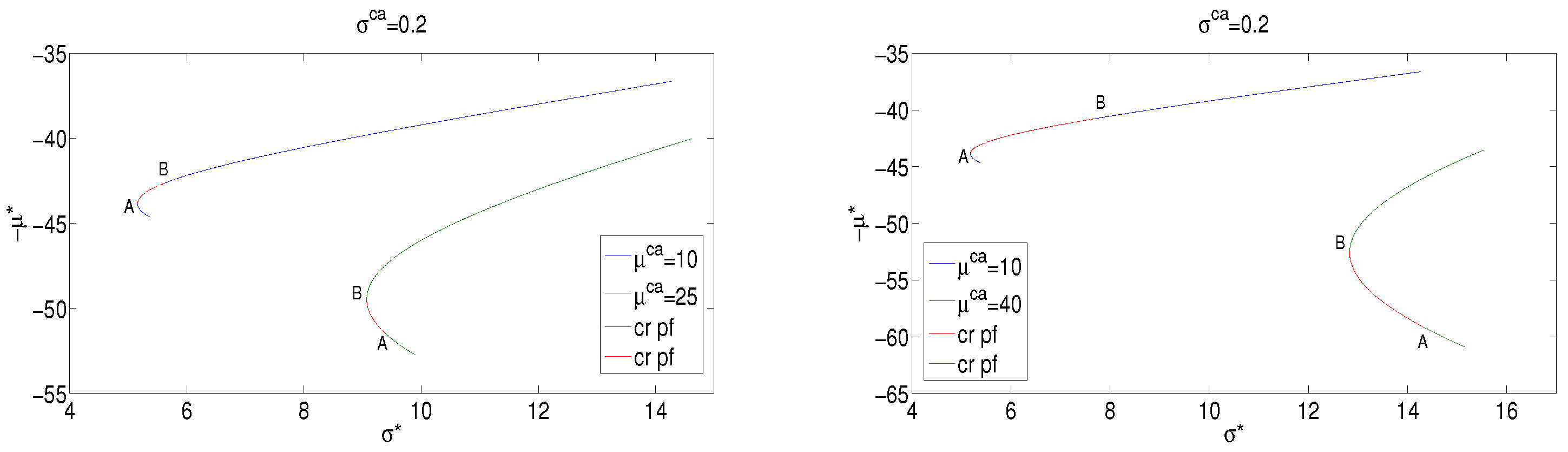
2.3. Optimal Systemic Portfolios

Equation (16) has two important consequences. First, it implies that all the portfolios belonging to the same subset $\varphi$ bear the same amount of risk (as measured by standard deviation or CVaRD of the stochastic EEC). In fact, Equation (16) shows that the risk of a feasible portfolio depends only on the first two terms in the r.h.s. and does not depend on operating capacity factors. Second, in each subset $\varphi$ of the technically feasible set ($0<\varphi <1$), we can select an optimum portfolio that stochastically dominates all the portfolios belonging to the same subset, i.e., such that

$$S_{\varphi }^{*}\left(\omega \right)\le S_{\varphi }^{\mathrm{sys}}\left(\omega \right),$$

(17)

for all systemic portfolios belonging to the subset (if $\varphi =0$ or $\varphi =1$, the corresponding subset of the technically feasible set contains a unique portfolio consisting of wind and a single fossil source, namely coal for $\varphi =0$ and gas for $\varphi =1$). In fact, since $B^{\mathrm{co}}/{\overline{CF}}^{\mathrm{co}}>B^{\mathrm{ga}}/{\overline{CF}}^{\mathrm{ga}}$ (the coal technology has higher fixed investment costs with respect to the gas technology), using the data reported in Table A1, we obtain

$${\displaystyle \frac{B^{\mathrm{ga}}}{{\overline{CF}}^{\mathrm{ga}}}}=5.2,{\displaystyle \frac{B^{\mathrm{co}}}{{\overline{CF}}^{\mathrm{co}}}}=20.3.$$

(18)

Such an optimum is obtained by maximizing the operating capacity factor of coal plants $C{F}^{\mathrm{co}}$, that is by making it equal to ${\overline{CF}}^{\mathrm{co}}$. The optimum portfolio is therefore characterized by the following operating capacity factors:

$$\begin{array}{cc}\hfill C{F}_{\varphi }^{\mathrm{ga}}& ={\displaystyle \frac{\varphi (1-{\overline{w}}^{\mathrm{wi}})C{F}^{\mathrm{sys}}}{1-c_v-(1-\varphi )(1-{\overline{w}}^{\mathrm{wi}}){\displaystyle \frac{C{F}^{\mathrm{sys}}}{{\overline{CF}}^{\mathrm{ga}}}}}},\hfill \\ \hfill C{F}_{\varphi }^{\mathrm{co}}& ={\overline{CF}}^{\mathrm{co}},\hfill \\ \hfill C{F}_{\varphi }^{\mathrm{wi}}& ={\overline{CF}}^{\mathrm{wi}},\hfill \end{array}$$

(19)

and by the following power capacity composition

$$\begin{array}{cc}\hfill W_{\varphi }^{\mathrm{ga}}& =\left[1-c_v-(1-\varphi )(1-{\overline{w}}^{\mathrm{wi}}){\displaystyle \frac{C{F}^{\mathrm{sys}}}{{\overline{CF}}^{\mathrm{ga}}}}\right]W^{\mathrm{sys}},\hfill \\ \hfill W_{\varphi }^{\mathrm{co}}& =(1-\varphi )(1-{\overline{w}}^{\mathrm{wi}}){\displaystyle \frac{C{F}^{\mathrm{sys}}}{{\overline{CF}}^{\mathrm{co}}}}{W}^{\mathrm{sys}},\hfill \\ \hfill W_{\varphi }^{\mathrm{wi}}& ={\overline{w}}^{\mathrm{wi}}{\displaystyle \frac{C{F}^{\mathrm{sys}}}{{\overline{CF}}^{\mathrm{wi}}}}{W}^{\mathrm{sys}},\hfill \end{array}$$

(20)

as it can be shown by substituting Equation (19) into Equation (10) and using Equation (11). The stochastic EEC of the optimal systemic portfolio belonging to the subset $\varphi$ is given by

$$\begin{array}{cc}\hfill S_{\varphi }^{*}\left(\omega \right)& =\varphi (1-{\overline{w}}^{\mathrm{wi}})A^{\mathrm{ga}}\left(\omega \right)+(1-\varphi )(1-{\overline{w}}^{\mathrm{wi}})A^{\mathrm{co}}\left(\omega \right)+\hfill \\ \hfill +& (1-\varphi )(1-{\overline{w}}^{\mathrm{wi}})\left({\displaystyle \frac{B^{\mathrm{co}}}{{\overline{CF}}^{\mathrm{co}}}}-{\displaystyle \frac{B^{\mathrm{ga}}}{{\overline{CF}}^{\mathrm{ga}}}}\right)+(1-c_v){\displaystyle \frac{B^{\mathrm{ga}}}{C{F}^{\mathrm{sys}}}}+{\overline{w}}^{\mathrm{wi}}{\overline{S}}^{\mathrm{wi}}.\hfill \end{array}$$

(21)

Equations (19)–(21), provide a complete technical characterization of the optimal systemic portfolio belonging to the subset $\varphi$ of the technically feasible set. As $\varphi$ varies between 0 and 1, we obtain a complete characterization of all optimal systemic portfolios for a given power system. Equation (21) can be also cast in the following, more expressive, form

$$\begin{array}{cc}\hfill S_{\mathsf{\Phi }}^{*}\left(\omega \right)=\varphi (1-{\overline{w}}^{\mathrm{wi}})& {\overline{S}}^{\mathrm{ga}}\left(\omega \right)+(1-\varphi )(1-{\overline{w}}^{\mathrm{wi}}){\overline{S}}^{\mathrm{co}}\left(\omega \right)+{\overline{w}}^{\mathrm{wi}}{\overline{S}}^{\mathrm{wi}}+\hfill \\ \hfill +& \left[{\displaystyle \frac{1-c_v}{C{F}^{\mathrm{sys}}}}-{\displaystyle \frac{1-{\overline{w}}^{\mathrm{wi}}}{{\overline{CF}}^{\mathrm{ga}}}}\right]B^{\mathrm{ga}}.\hfill \end{array}$$

(22)

Equation (22) shows that the optimal stochastic EEC in the subset $\varphi$ can be determined as an affine combination of single technology EECs, computed at their nominal capacity factors, augmented of a term accounting for the constraints imposed by the yearly load duration curve, the intermittent renewables availability and by the capacity value of the power system.

3. The Dynamics of Stochastic Factors: A DNN-Based Model

The stochastic EEC enters the portfolio selection problem via its probability distribution and its moments. In the proposed approach, the EEC probability distribution depends on three stochastic factors, namely the price of fossil fuels (gas and coal) and the price of carbon. An appropriate dynamic model must take into account the main facts of the three stochastic factors and, possibly, their interactions and statistical correlations. Once the model is identified, the evolution paths of the stochastic factors are obtained through Monte Carlo simulations, and EEC values are calculated along these paths.

3.1. Modeling the Joint Dynamics of Gas and Coal

The dynamics of gas and coal prices are modeled taking into account the market values of the underlying financial processes, and, possibly, their statistical correlations. To perform this task, we adopt a distributional approach as far as the joint process of the dynamics of the fossil fuel components is considered, in which the joint transition probability distribution of gas and coal prices, conditional on histories, is numerically estimated. Noticeably, using a standard linear econometric approach, the conditional joint cumulative distribution corresponding to the sought density could be obtained by a conditional quantile regression [53] for a given selection of quantiles fitted to data. However, price stationarity would be required, and, most importantly, nonlinearity would be lost. As a better approach, we chose to use a Deep Neural Network (DNN) with a Softmax function in the last dense layer. The set of network weights are adjustable parameters, and the components of the Softmax function can be interpreted as components of a discretized joint probability distribution over price bins.

In the training dataset, each input observation is made up of a couple of numbers $z_i=(X_i^{\mathrm{ga}},X_i^{\mathrm{co}})$, which are, respectively, the gas and coal prices (expressed in USD per mmBtu) relative to the time i. Each element of the training dataset is composed of n$(<N)$ consecutive input observations on which LSTM layers operate, $z_k,z_{k+1},\cdots ,z_{k+n-1}$, with $k=1,2,\cdots ,N-n$, and one output observation, namely $z_{k+n}$. The reason we considered price pairs in the training dataset is that these two markets can exhibit correlation. Training (i.e., optimizing) the network on data can return, in a very direct way, a more satisfactory single-period conditional joint probability density. In addition, the deeper the network (to a point, in order to avoid overfitting), the more accurate the estimation of the distribution and of the statistical interactions between the fossil fuel components. If we denote by

$${\mathbf{z}}_{t-1,t-n}=\{z_{t-1},z_{t-2},\cdots ,z_{t-n}\},$$

(23)

a sequence of temporally ordered input observations, the Softmax function returns the single-period conditional joint transition probability

$$p\left(z_t\right|{\mathbf{z}}_{t-1,t-n}).$$

(24)

In fact, since Softmax returns a vector of non-negative numbers that sum to one, it is possible to interpret these non-negative numbers as conditional joint transition probabilities of the DNN outcome.

Hence, as a density estimator, we employed a DNN with a multilayer architecture characterized by nine layers, arranged in the following sequence: an input layer, to which the two-price input is fed; an initial embedding layer; two smoothing stacks composed of a convolutional layer and a max pooling layer; two Long Short-Term Memory (LSTM) layers (acting along the temporal dimension of the input vectors only), and one dense layers for output. Notice that in this way, the LSTMs run along the n steps of each data sample and not along the whole training dynamics. The DNN architecture is depicted in Figure 2.

We designed this DNN to account for the main facts of observed energy commodity price dynamics, such as mean reversion and the presence of jumps and spikes. Among all the stylized properties of the dynamics of commodity prices, mean reversion is the one that needs to be given the most attention because it requires consideration of the interactions between the short-run and long-run dynamics. To account for this, we designed a DNN hybrid architecture consisting of a combination of convolutional layers, long short-term memory (LSTMs), and fully connected layers for final processing and decision-making. This combination is particularly effective in modeling commodity price time series because it captures both short-term fluctuations and long-term dependencies, which are critical for understanding the mean-reverting market dynamics [44]. Specifically, convolutional layers for feature extraction provide the model with the ability to detect short-term market patterns and efficiently extract local patterns and price movements, including extreme events such as jumps and spikes. Then, identified local patterns are passed to the LSTM layers, which excel at maintaining memory over extended time periods, allowing the model to handle long-term dependencies.

This architecture is designed to capture the nonlinear relationships that exist between temporally ordered observations [54]. In this configuration, the smoothing of input data is performed by two layer sequences consisting of a convolutional layer and a max pooling layer, stacked one after the other. The presence of these two sequences of layers is intended to more accurately approximate the nonlinear relationships between the input data, thereby obtaining better feature representations [55]. In the convolutional layers, a Rectified Linear Unit (ReLU) is used as an activation function. Then, the features are passed to the two LSTM layers, which are stacked on top of each other to improve the performance [56]. Recurrent neural networks such as LSTM showed strong performance due to their ability to process data sequences and capture the temporal dependencies within the inputs [43]. The probabilistic prediction task is then completed by the last dense layer in which Softmax is used as the activation function.

Table 1. DNN main parameters.

Layer	Parameters
Input	shape = $2n$
Embedding	input_dim = 40,000, output_dim = 100, input_length = $2n$
Convolutional	filters = 128, kernel_size = 5, activation = ReLU
MaxPooling	pool_size = 2
Convolutional	filters = 64, kernel_size = 5, activation = ReLU
MaxPooling	pool_size = 2
LSTM	units = 256, dropout = 0.2
LSTM	units = 128, dropout = 0.1
Dense	units = ${\Delta }^{\mathrm{ga}}\times {\Delta }^{\mathrm{co}}$, activation = Softmax

provides the DNN parameters (Tensorflow 2.7.0 library for Python 3.9 is used).

To compute the loss, we used the Sparse Categorical Crossentropy function together with the Adam optimizer.

The DNN was trained on the whole period for six hundred epochs, assuming $n=10$ [54]. The computational cost proved to be negligible. Training was completed in a few minutes on an NVIDIA H100, demonstrating the efficiency and computational scalability of the approach. To validate its portability across different computational environments, we replicated the experiment on a GTX 1070 Ti, a widely available consumer-grade GPU, where training was completed in approximately one hour. This confirms that, while the model scales effectively on high-performance hardware, it remains practical and easily trainable on more accessible computational resources.

In order to implement the generative approach followed in this study, we first defined the appropriate binning range ${\Delta }^{\mathrm{ga}}$ for gas prices and ${\Delta }^{\mathrm{co}}$ for coal prices. In our specific approach, all the values of the detrended real gas and coal price time series are used to define the binning range, from the minimum to the maximum observed value. Our dataset consists of the monthly time series of gas and coal prices since January, 1999 until December, 2019. The data refer to the cost of natural gas and coal receipts at electric generation plants. Then, a different bin (class) is associated with each value belonging to the binning range, rounded to two decimal places. Once the DNN is trained, the conditional joint transition probability distribution can be estimated. It should be noted that the proposed approach does not require the time series to be stationary. This fact is another strength that allows the potential of this method to be extended to many other areas of application. Knowledge of the conditional joint transition probabilities enables the construction of a stochastic process based on the DNN. In fact, by randomly sampling the DNN output price bins via Monte Carlo techniques based on estimated single-period conditional joint probabilities $p\left(z_t\right|{\mathbf{z}}_{t-1,t-n})$, in a sliding-window manner, the DNN can generate synthetic paths of the underlying stochastic processes for gas and coal prices. Based on the expected growth rate of fossil fuel prices given in the AEO 2016 [48], a real annual escalation rate of $2\%$ for gas prices and $0.3\%$ for coal prices was included in the path generation process.

DNN Validation and Performance Evaluation

The design of the DNN was guided by the need to balance model complexity, training efficiency, and predictive accuracy. Specifically, the dataset was split into a training period spanning from January, 1999 to December, 2015, and the validation period was from January, 2016 to December, 2019. The DNN configuration was assessed by evaluating its ability to reconstruct the time series over the validation period. As an evaluation metric, we used the Mean Absolute Error (MAE) computed between the observed in-sample time series and a randomly generated path from the DNN, defined as follows:

$${\mathrm{MAE}}_k={\displaystyle \frac{1}{k}}\sum _{j=1}^k|x_j-{\widehat{x}}_j|,$$

(25)

where $x_j$ is the j-th simulated value from the DNN-generated path and ${\widehat{x}}_j$ is the corresponding observed value in the time series. The integer k represents the number of months of the validation period. The sample mean ${\overline{\mathrm{RMSE}}}_k$ was then computed by averaging ${\mathrm{RMSE}}_k$ over one thousand randomly generated paths. Extensive testing and hyperparameter tuning were conducted to ensure robustness and reproducibility. We performed a systematic grid search over multiple combinations of hyperparameters, including the number of units in the first LSTM layer $(128,256,512)$ (while the number of units in the second LSTM layer was set as equal to half the units in the first layer) convolutional kernel sizes $(3,5,7)$, and dropout rates $(0.1,0.2,0.3)$.

Our sensitivity analysis revealed that increasing the number of units in the first LSTM layer from 128 to 512 improves accuracy but comes with a significant rise in computational cost. Doubling the number of LSTM units increased the training time by approximately $30\%$; however, beyond a certain threshold, further increases in model size provided diminishing returns in predictive performance. Specifically, we observed that increasing the first LSTM layer above 256 units (and the second layer above 128 units) resulted in an ${\overline{\mathrm{MAE}}}_k$ reduction of less than $1\%$ across all tested convolutional kernel sizes. Regarding dropout regularization, a value of 0.2 was found to be optimal, effectively preventing overfitting while maintaining learning efficiency. The convolutional layer kernel size of 5 provided the best trade-off between predictive performance and computational time, as increasing the kernel size from 3 to 7 led to a $20\%$ increase in training time without substantial gains in accuracy. Notably, removing the convolutional or LSTM layers individually resulted in performance degradation: ${\overline{\mathrm{MAE}}}_k$ increased by $13\%$ without convolutional layers and by $18\%$ without LSTM layers, underscoring the complementary roles of these components in capturing both local and long-term patterns in fossil fuel price dynamics.

3.2. Modeling the Dynamics of Carbon Prices

The dynamics of carbon (real) prices, expressed in USD per ton of CO₂, is modeled according to a geometric Brownian motion of the type

$${\displaystyle \frac{d{X}_t^{\mathrm{ca}}}{X_t^{\mathrm{ca}}}}={\sigma }^{\mathrm{ca}}d{Z}_t^{\mathrm{ca}},$$

(26)

where ${\sigma }^{\mathrm{ca}}$ is the carbon volatility and $Z_t^{\mathrm{ca}}$ is a standard Brownian motion. Assuming that the dynamic of CO₂ prices is described by a geometric Brownian motion with zero drift implies that the stochastic process $X_t^{\mathrm{ca}}$ has a constant mean ${\mu }^{\mathrm{ca}}$ that coincides with the initial condition of the CO₂ price process, namely ${\mu }^{\mathrm{ca}}=X_0^{\mathrm{ca}}$. While this is a simplified assumption, it is economically grounded. Since our analysis operates in real terms (deflated prices), the assumption of zero drift means that in the nominal economy, expected carbon prices grow exponentially with the inflation rate. The assumption of zero drift is, therefore, consistent with the broader economic context. We acknowledge the existence of more complex stochastic processes in the literature, such as mean-reverting models (e.g., Ornstein–Uhlenbeck processes) and jump-diffusion frameworks. These could offer a more nuanced representation of CO₂ markets influenced by policy shocks and abrupt regulatory changes. However, our goal is to isolate and study the impact of price volatility per se, rather than directional trends or discrete regime changes. Future work will explore these richer dynamics as extensions of the current framework.

In the following, we refer to ${\mu }^{\mathrm{ca}}$ as the CO₂ price level. To investigate the impact of CO₂ price volatility on power system portfolio selection and on CO₂ emission management, we consider three different volatility scenarios characterized by ${\sigma }^{\mathrm{ca}}=0,20\%,30\%$. This assumption tries to depict a zero volatility, a medium, and a high volatility scenario, respectively, in which we can investigate the combined effects of CO₂ price level and CO₂ price volatility on assessing risk and CO₂ emissions. To do this, three different CO₂ price level are used, namely ${\mu }^{\mathrm{ca}}=10,25,40$ USD-2015 per ton of CO₂. $X_t^{\mathrm{ga}}$, $X_t^{\mathrm{co}}$ and $X_t^{\mathrm{ca}}$ enter in the variable costs terms $A^{\mathrm{ga}}\left(\omega \right)$ and $A^{\mathrm{co}}\left(\omega \right)$ of Equation (27). The stochastic dynamics of carbon prices $X_t^{\mathrm{ca}}$ therefore affects the variable costs of both gas and coal technologies, thus introducing a correlation between their stochastic EECs. Under this setting, stochastic variable costs can be written as a linear combination of a fuel and a carbon contribution, namely

$$A^x\left(\omega \right)={\displaystyle \frac{H^x}{1000M}}\sum _{n=1}^M{X}_n^x\left(\omega \right)F_{0,n}+{\displaystyle \frac{K^x}{M}}\sum _{n=1}^M{X}_n^{\mathrm{ca}}\left(\omega \right)F_{0,n}+D^x,$$

(27)

where $H^x$ is the fuel heat rate and $K^x$ is the CO₂ intensity (expressed in tCO₂ per MWh). $D^x$ is the deterministic component of the variable costs accounting for O&M variable costs. Declaring $D^x$ deterministic in Equation (27) implies that we assumed that other costs have a negligible variance with respect to fuel costs and CO₂ prices volatility.

The empirical EEC distribution of systemic portfolios can be obtained by using Monte Carlo techniques. For each run of the Monte Carlo simulation, an evolution path for fossil fuel prices and carbon prices is obtained and, along such paths, EEC values are calculated. In this setting, the wind EEC is non stochastic and, using the data shown in Table A1, is given by ${\overline{S}}^{\mathrm{wi}}=23.5$ (USD-2015/MWh).

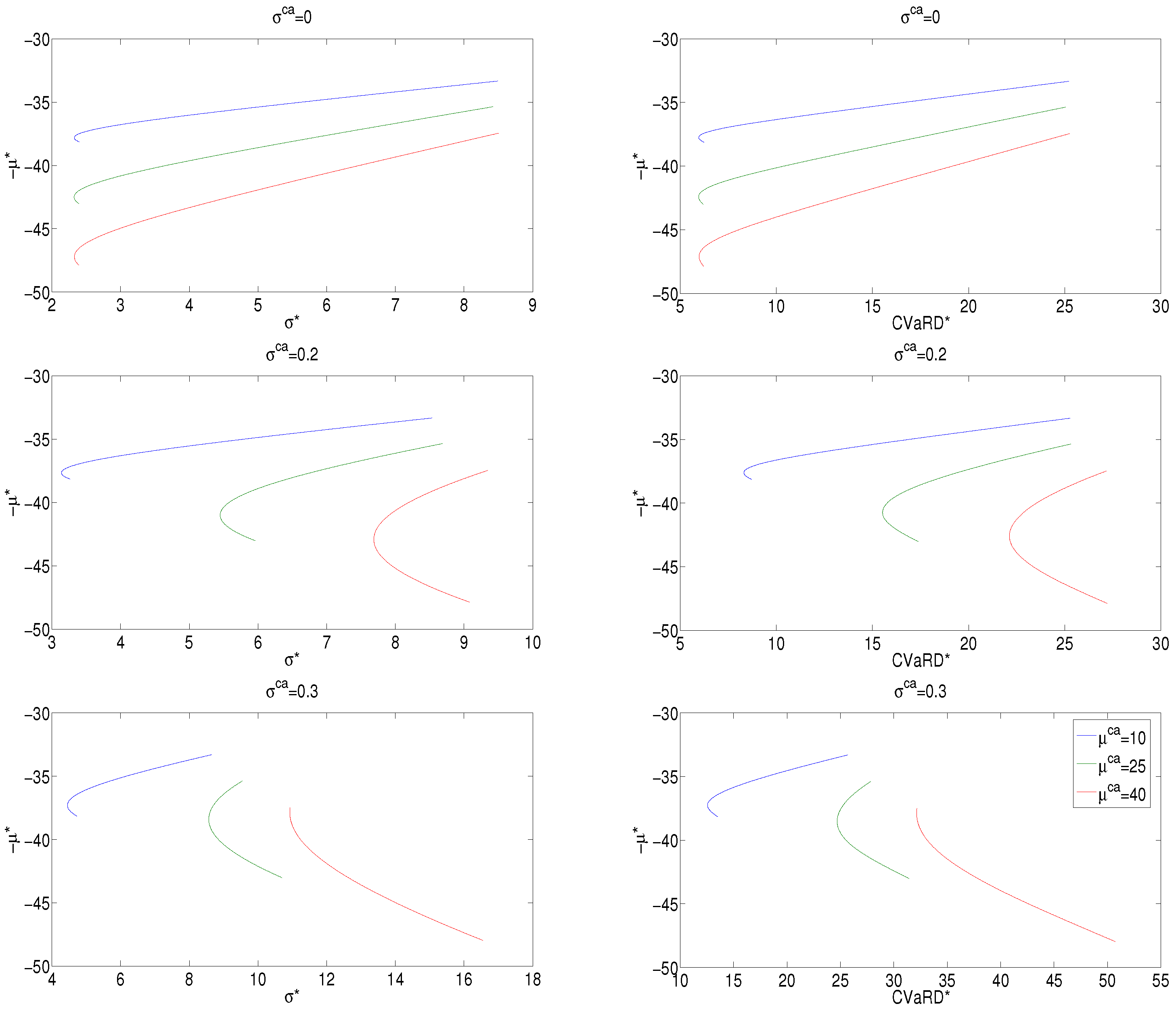
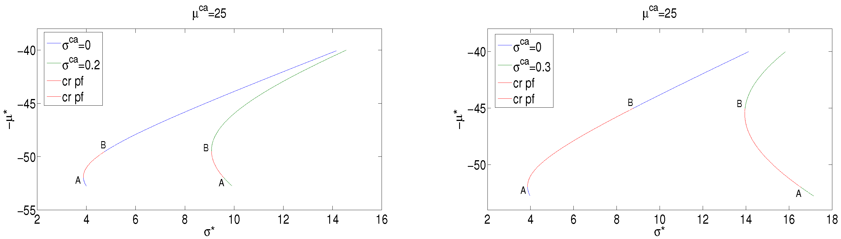
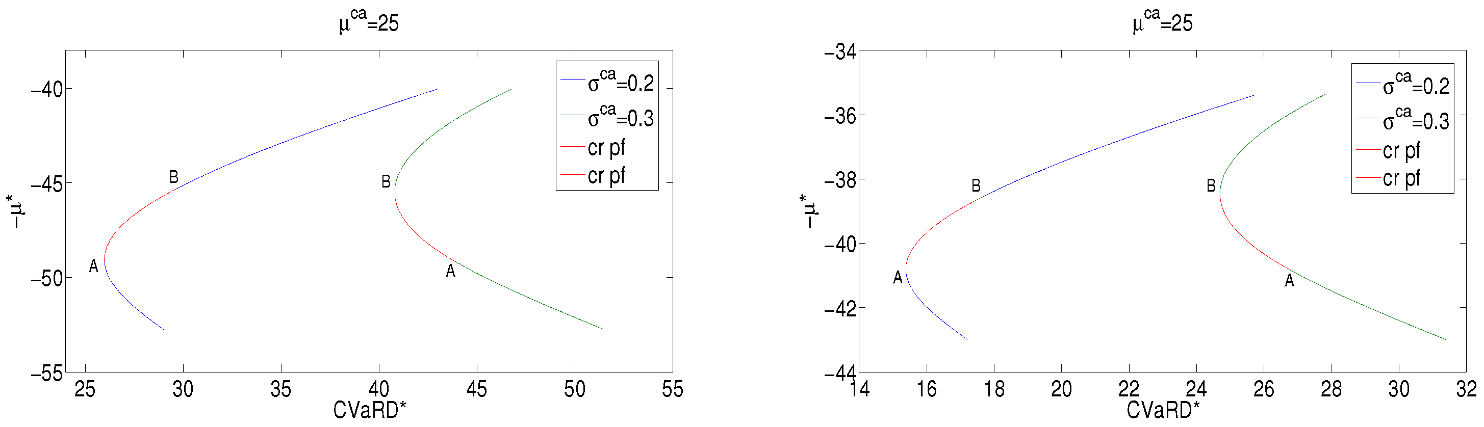
4. CO₂ Price Volatility and Emission Management

Systemic portfolio frontiers are the natural context in which to discuss the effects of CO₂ price volatility for carbon management. Systemic portfolios frontiers are determined using Equation (22) under a two-step procedure. First, for each subset $\varphi$, we compute the EEC mean and the measured risk values (standard deviation and CVaRD values) of the optimal systemic portfolio of that subset. Then, the systemic standard deviation frontier is obtained by plotting EEC mean and standard deviation values of optimal systemic portfolios for $0\le \varphi \le 1$. In the same way, the systemic CVaRD frontier is obtained by computing EEC mean and CVaRD values of optimal systemic portfolios.

Figure 3 displays systemic frontiers for $c_v=0.1$ and $C{F}^{\mathrm{sys}}=0.7$, in the three CO₂ price volatility scenarios characterized by ${\sigma }^{\mathrm{ca}}=0,20\%,30\%$ for ${\mu }^{\mathrm{ca}}=10,25,40$. In the case of CVaRD, the confidence level has been chosen as equal to $95\%$. The wind penetration has been chosen as equal to ${\overline{w}}^{\mathrm{wi}}=0.4$, in agreement with the US planned target reported in the ‘Renewable Electricity Futures Study’ published by the National Renewable Energy Laboratory [57]. Also documented in the ‘IEA Wind—2023 Annual Report’ [58], several European countries have similar targets, and Denmark reached a wind penetration of $54.1\%$ in 2023.

The efficient systemic portfolio frontier (or simply the efficient frontier) is represented by the upward sloping portion of the curve that starts with the minimum variance portfolio (mvp) or minimum CVaRD (mcp) and ends with the portfolio consisting of only gas and wind. Moving from right to left along the efficient frontier, the gas component increases and, consequently, the coal component decreases, thus reducing the CO₂ emission rate. Moving from right to left also reduces the generation costs and increases risk. We call efficient systemic portfolios (or simply efficient) the optimal systemic portfolios belonging to the efficient frontier.

We notice from Equation (21) that the capacity value does not affect the risk of the systemic frontier portfolios but it influences EEC mean values.

Table 2. Composition of mvp systemic portfolios. CO₂ emission rates of these portfolios are also shown.

${\mathit{\sigma }}^{\mathbf{ca}}$	Technology	${\mathit{\mu }}^{\mathbf{ca}}=10$	${\mathit{\mu }}^{\mathbf{ca}}=25$	${\mathit{\mu }}^{\mathbf{ca}}=40$
0	wi	40%	40%	40%
	ga	6%	6%	6%
	co	54%	54%	54%
$E_{\mathrm{mvp}}^{{\mathrm{CO}}_2}$		0.470	0.470	0.470
0.20	wi	40%	40%	40%
	ga	8%	18%	31%
	co	52%	42%	29%
$E_{\mathrm{mvp}}^{{\mathrm{CO}}_2}$		0.461	0.413	0.350
0.30	wi	40%	40%	40%
	ga	13%	39%	59%
	co	47%	21%	1%
$E_{\mathrm{mvp}}^{{\mathrm{CO}}_2}$		0.437	0.312	0.215

and

Table 3. Composition of mcp systemic portfolios. CO₂ emission rates of such portfolios are also shown.

${\mathit{\sigma }}^{\mathbf{ca}}$	Technology	${\mathit{\mu }}^{\mathbf{ca}}=10$	${\mathit{\mu }}^{\mathbf{ca}}=25$	${\mathit{\mu }}^{\mathbf{ca}}=40$
0	wi	40%	40%	40%
	ga	6%	6%	6%
	co	54%	54%	54%
$E_{\mathrm{mcp}}^{{\mathrm{CO}}_2}$		0.470	0.470	0.470
0.20	wi	40%	40%	40%
	ga	9%	19%	32%
	co	51%	41%	28%
$E_{\mathrm{mcp}}^{{\mathrm{CO}}_2}$		0.456	0.408	0.345
0.30	wi	40%	40%	40%
	ga	14%	37%	58%
	co	46%	23%	2%
$E_{\mathrm{mcp}}^{{\mathrm{CO}}_2}$		0.432	0.321	0.220

depict, respectively, the composition of both the mvp and mcp systemic portfolios in the various scenarios. CO₂ emission rates, expressed in $tC{O}_2$ per MWh and computed using Equation (28), are also shown.

In the zero CO₂ volatility scenario (i.e., under a deterministic carbon tax), the CO₂ price level ${\mu }^{\mathrm{ca}}$ has no effect on the risk of systemic portfolios. In particular, the composition of the mvp and mcp portfolios is invariant under changes in ${\mu }^{\mathrm{ca}}$ (see Table 2 and Table 3), and, consequently, the entire efficient frontier is invariant. Figure 3 shows in the upper panel that the only effect of changes in ${\mu }^{\mathrm{ca}}$ is an increase in the EEC mean, and the efficient frontiers move south. Under volatile CO₂ scenarios, the picture is very different. In this case, Table 2 and Table 3 show that the composition of mvp and mcp portfolios is influenced by the CO₂ price level ${\mu }^{\mathrm{ca}}$. Specifically, as ${\mu }^{\mathrm{ca}}$ increases, the gas component in both mvp and mcp portfolios increases and, consequently, the coal component decreases, thus reducing the CO₂ emission rate. Consequently, under volatile CO₂ scenarios, all efficient systemic portfolios will be characterized by decreasing CO₂ emission rates as ${\mu }^{\mathrm{ca}}$ increases. In this sense, the joint effect of non-zero CO₂ price volatility and CO₂ price level reduces CO₂ emissions in the power sector. CO₂ price volatility can be, therefore, seen as a mitigating factor. In fact, in scenarios with higher CO₂ price volatility, optimal portfolios systematically reduce the reliance on coal, a high-emission source, in favor of gas. This shift occurs as a risk-averse response to increased uncertainty, leading to lower expected emissions even without explicit emission targets. In the absence of price volatility (i.e., under a deterministic carbon tax), the CO₂ price level influences only the cost of portfolios, not their risk profile. Consequently, static pricing mechanisms may fail to incentivize cleaner energy mixes. However, great care must be taken because the combined effect of high values of both volatility and CO₂ price could drastically reduce the efficient frontier (even to a single point, i.e., mvp or mcp). This effect is clearly shown in the bottom panel of Figure 3.

The planning choice is not necessarily represented by the mvp or the mcp portfolio. Since each systemic portfolio belonging to the systemic efficient portfolio frontier is an efficient EEC mean-risk choice, the energy planner can use this degree of freedom for energy policy purposes in order to determine the optimum power system portfolio. Hence, a CO₂ emission control variable can be introduced to fix a target on CO₂ emissions in the power sector. Let us recall that the CO₂ emission rate of a generation portfolio (measured, for example, in tCO₂ per MWh) is a linear combination of single technology emission rates, using as weights the fraction of energy generated by each single technology. Hence, all systemic portfolios belonging to the subset $\varphi$ are characterized by the same emission rate (measured, for example, in $tC{O}_2$ per MWh)

$$E_{\varphi }^{{\mathrm{CO}}_2}=\varphi (1-{\overline{w}}^{\mathrm{wi}})E^{{\mathrm{CO}}_{2,\mathrm{ga}}}+(1-\varphi )(1-{\overline{w}}^{\mathrm{wi}})E^{{\mathrm{CO}}_{2,\mathrm{co}}},$$

(28)

where $E^{{\mathrm{CO}}_{2,\mathrm{ga}}}$ and $E^{{\mathrm{CO}}_{2,\mathrm{co}}}$ are, respectively, the CO₂ emissions rates of the gas and the coal technologies. In the empirical analysis, emissions rates are computed using the values $E^{{\mathrm{CO}}_2,1}=0.351$ tCO₂/MWh and $E^{{\mathrm{CO}}_2,2}=0.832$ tCO₂/MWh (see Table A1).

This fact implies that the optimum portfolio of the subset $\varphi$ is optimal also for CO₂ emissions. A target value $E_{\mathrm{opt}}^{{\mathrm{CO}}_2}$ on the CO₂ emission rate can determine uniquely the composition of the optimum power system portfolio, namely

$${\varphi }_{\mathrm{opt}}={\displaystyle \frac{(1-{\overline{w}}^{\mathrm{wi}})E^{{\mathrm{CO}}_{2,\mathrm{co}}}-E_{\mathrm{opt}}^{{\mathrm{CO}}_2}}{(1-{\overline{w}}^{\mathrm{wi}})\left(E^{{\mathrm{CO}}_{2,\mathrm{co}}}-E^{{\mathrm{CO}}_{2,\mathrm{ga}}}\right)}}.$$

(29)

In this way, the power system portfolio selection problem admits a unique solution that optimally combines risk, costs, CO₂ emissions and include in an efficient way all the wind energy available in the power system.

Table 4. Composition of optimal systemic portfolios with assigned target values of CO₂ emission rates $E_{\mathrm{opt}}^{{\mathrm{CO}}_2}$.

Technology	${\mathit{E}}_{\mathbf{opt}}^{{\mathbf{CO}}_2}=0.45$	${\mathit{E}}_{\mathbf{opt}}^{{\mathbf{CO}}_2}=0.40$	${\mathit{E}}_{\mathbf{opt}}^{{\mathbf{CO}}_2}=0.35$	${\mathit{E}}_{\mathbf{opt}}^{{\mathbf{CO}}_2}=0.30$	${\mathit{E}}_{\mathbf{opt}}^{{\mathbf{CO}}_2}=0.25$
wi	40%	40%	40%	40%	40%
ga	10%	21%	31%	41%	52%
co	50%	39%	29%	19%	8%

depicts the composition of optimal systemic portfolios with assigned target values of CO₂ emission rates.

As a further illustrative example, suppose we set the target value $E_{\mathrm{opt}}^{{\mathrm{CO}}_2}=0.360$ (tCO₂/MWh). Such a value corresponds to ${\varphi }_{\mathrm{opt}}=0.48$. Figure 4 shows the EEC sample distributions of the optimal systemic portfolio belonging to the subset ${\varphi }_{\mathrm{opt}}=0.48$ of the technically feasible set for a power system with $c_v=0.1$, $C{F}^{\mathrm{sys}}=0.7$ and ${\overline{w}}^{\mathrm{wi}}=0.4$.

Table 5. First two moments of $S_{0.48}^{*}\left(\omega \right)$.

${\mathit{\sigma }}^{\mathbf{ca}}$	${\mathit{\mu }}^{\mathbf{ca}}$	${\mathit{\mu }}_{0.48}^{*}$	${\mathit{\sigma }}_{0.48}^{*}$
0	10	35.9	4.2
	25	39.4	4.2
	40	42.9	4.2
0.2	10	35.9	4.6
	25	39.4	5.8
	40	42.9	7.7
0.3	10	35.9	5.2
	25	39.4	8.8
	40	42.9	12.4

reports the first two moments of the EEC simulated distribution in each carbon volatility scenario for ${\mu }^{\mathrm{ca}}=10,25,40$.

Economic and Policy Implications

Our results indicate that the CO₂ price volatility plays a crucial role in the CO₂ emission reduction process because if forces an efficient reduction of the coal component of power generation portfolios for risk-aversion reasons. This is an important indication for a policymaker concerned with environmental issues besides economic issues [25].

Energy planners have to pay great attention when they project CO₂ pricing mechanisms. Systemic efficient frontiers are, in fact, very sensitive to the dynamical parameter of the CO₂ price evolution, namely the CO₂ price level ${\mu }^{\mathrm{ca}}$ and CO₂ price volatility ${\sigma }^{\mathrm{ca}}$. The planning choice is, therefore, strongly influenced by these parameters. As we have shown in this study, a deterministic carbon tax does not modify the risk profile of optimal systemic portfolios and may have no effects on CO₂ emission reduction. On the other side, high values of CO₂ price volatility drastically reduce the efficient frontier, especially for high values of the CO₂ price level. These two parameters must be continuously monitored and adequately controlled. What are, then, the consequences of a non-adequate planner’s view of the CO₂ pricing mechanism?

Figure 3 shows that there exist optimal systemic portfolios that are efficient in a given CO₂ price volatility scenario, but which become inefficient in an another CO₂ price volatility scenario. We call critical portfolio an optimal systemic portfolio with this property. The concept of critical portfolios illustrates the importance of aligning policy assumptions with market realities. Misjudging CO₂ volatility or price levels can lead to inefficient and environmentally suboptimal decisions. Figure 5, Figure 6, Figure 7 and Figure 8 provide meaningful examples.

Figure 5 depicts systemic mean-standard deviation frontiers for dispatchable only sources (${\overline{w}}^{\mathrm{wi}}=0$) in the case ${\mu }^{\mathrm{ca}}=25$ for different CO₂ volatility scenarios, namely ${\sigma }^{\mathrm{ca}}=0$ and ${\sigma }^{\mathrm{ca}}=20\%$ (left panel) and ${\sigma }^{\mathrm{ca}}=0$ and ${\sigma }^{\mathrm{ca}}=30\%$ (right panel).

Portfolio A is the mvp portfolio in the non-volatile carbon tax scenario. Under volatile CO₂ scenarios, portfolio A becomes an inefficient choice. In fact, such a portfolio is located in the red part of the green systemic frontier. The mvp and all portfolios belonging to the red portion of the blue frontier, from portfolio A to portfolio B, are located in the red portion of the green frontier and become inefficient choices. On the other hand, high values of CO₂ price volatility reduce the planner choice set. Figure 6 depicts systemic mean-CVaRD frontiers for dispatchable only sources (left panel) and in the case in which the wind source is included in the power system (right panel) for ${\mu }^{\mathrm{ca}}=25$ in the two CO₂ volatility scenarios ${\sigma }^{\mathrm{ca}}=20\%$ and ${\sigma }^{\mathrm{ca}}=0.30\%$. In this case, A is the mcp portfolio in the ${\sigma }^{\mathrm{ca}}=20\%$ scenario. Since the planner choice can regard only efficient systemic portfolios belonging to the green frontier (the high volatility scenario), critical portfolios (the red portion of the green frontier) which would be efficient under lower CO₂ price volatility levels (the red portion of the blue frontier) are excluded by the choice set.

Figure 7 depicts systemic frontiers for dispatchable only sources (${\overline{w}}^{\mathrm{wi}}=0$) in the case ${\sigma }^{\mathrm{ca}}=20\%$ for different CO₂ price level scenarios, namely ${\mu }^{\mathrm{ca}}=10$ and ${\mu }^{\mathrm{ca}}=25$ (left panel) and ${\mu }^{\mathrm{ca}}=10$ and ${\mu }^{\mathrm{ca}}=40$ (right panel).

Finally, Figure 8 illustrates the consequences of combining different estimates of CO₂ price levels with different CO₂ price volatility scenarios.

The findings highlight how CO₂ price volatility, often considered a risk factor, can become a strategic lever for emission mitigation when properly understood and incorporated into planning frameworks. Introducing CO₂ price volatility through market-oriented mechanisms (e.g., cap-and-trade systems like the EU ETS) can act as a de facto emission reduction policy. In fact, market-oriented mechanisms can play an important role in revealing the dynamics of CO₂ prices, thus providing correct signals to energy planners and policymakers who face the problem of power system portfolio selection. Volatility sends stronger signals to planners and investors than a deterministic carbon tax. These results suggest that energy planners and policymakers should view CO₂ price volatility not as a source of instability to be minimized, but as a potential regulatory lever that aligns market behavior with environmental objectives. Rather than pursuing rigid pricing schemes, policymakers might benefit from designing adaptive, market-informed instruments that reveal the underlying CO₂ dynamics and guide the transition toward low-carbon power systems. Through appropriate incentive schemes, policymakers will have the opportunity to guide investments toward power system configurations that optimally combine risk, cost, and CO₂ emissions. The methodology proposed in this study offers a quantitative basis for evaluating such mechanisms under a variety of market conditions.

5. Conclusions

This paper proposes a novel methodological framework for power system portfolio optimization under uncertainty, integrating the deep learning-based forecasting and stochastic modeling of carbon prices. By combining a supervised DNN-based stochastic model for fossil fuel prices with a stochastic process for CO₂ price dynamics, we simulate a wide range of plausible market scenarios and assess the trade-offs among the cost, risk, and environmental impact from a societal planning perspective.

Our results highlight the critical role of CO₂ price volatility in shaping generation portfolios and reducing emissions. While a deterministic carbon tax affects only the cost of portfolios, a volatile CO₂ pricing mechanism acts as an implicit regulatory signal that incentivizes cleaner energy mixes even in the absence of explicit emission targets. This counterintuitive insight, that volatility can be environmentally beneficial, represents a valuable contribution to the ongoing debate on market-based versus fixed carbon pricing.

Finally, we introduced the concept of a CO₂ emission control variable, showing how the planner can use it to uniquely determine optimal systemic portfolios that efficiently integrate wind energy and balance cost, risk, and emissions. The combined effects of CO₂ price volatility, CO₂ price level, and rational choice reduce CO₂ emissions to an extent that can be quantified. Under a well-defined target regarding the CO₂ emission rate, the power system portfolio selection problem admits a unique solution that integrates in an efficient way all the non-dispatchable electricity generation available in a given power system and optimally combines risk, costs, and CO₂ emissions.

This offers a powerful and flexible tool for energy policy design in uncertain environments and underscores the importance of aligning regulatory frameworks with market realities to avoid inefficient or environmentally suboptimal planning outcomes. As the governments are the planner subjects for energy choices, they have the duty to promote coherent externalities, pricing mechanisms, and technologies which permit the energy policy targets, providing clear signals to direct private investments. Our analysis thus provides quantitative support for identifying, targeting, and evaluating public actions and interventions, with the aim of reconciling market logic with societal benefits.

Future research will aim to extend the proposed framework along several directions. First, we plan to incorporate post-2020 fossil fuel market data to evaluate the model performance when the DNN is trained on time intervals that contain periods of anomalous instability, including those shaped by recent geopolitical events and global supply chain disruptions. Second, we intend to experiment with alternative stochastic models for CO₂ price dynamics, such as mean-reverting processes and jump-diffusion models, to better capture regulatory shocks and market behavior. Third, we are exploring the possibility of including nuclear power generation from modular reactors, with the aim of studying the effects of CO₂ price volatility on optimal systemic portfolios in the presence of a dispatchable, carbon-free source. Finally, the integration of emerging renewable technologies and storage systems will be explored to enhance the applicability of our methodology to next-generation energy systems. Although this study is limited to established technologies and U.S.-based data, the methodology is generalizable and applicable to regions with different market structures and generation technologies. Future research could investigate the robustness of the proposed approach when applied to different energy markets, thereby extending its applicability and relevance.

References

1. Markowitz, H. Porfolio Selection. J. Financ. 1952, 7, 77–91. [Google Scholar]
2. Awerbuch, S.; Berger, M. Applying Portfolio Theory to EU Electricity Planning and Policy-Making; IEA/EET Working Paper EET/2003/03; International Energy Agency: Paris, France, 2003. [Google Scholar]
3. DeLlano-Paz, F.; Calvo-Silvosa, A.; Iglesias, S.; Soares, I. Energy planning and modern portfolio theory: A review. Renew. Sustain. Energy Rev. 2017, 77, 636–651. [Google Scholar] [CrossRef]
4. Joskow, P.L. Comparing the costs of intermittent and dispatchable electricity generating technologies. Am. Econ. Rev. 2011, 101, 238–241. [Google Scholar] [CrossRef]
5. Reichelstein, S.; Sahoo, A. Time of day pricing and the levelized cost of intermittent power generation. Energy Econ. 2015, 48, 97–108. [Google Scholar] [CrossRef]
6. Gómez Sánchez, M.; Macia, Y.M.; Fernández Gil, A.; Castro, C.; Nuñez González, S.M.; Pedrera Yanes, J. A Mathematical Model for the Optimization of Renewable Energy Systems. Mathematics 2021, 9, 39. [Google Scholar] [CrossRef]
7. Hittinger, E.; Whitacre, J.F.; Apt, J. Compensating for wind variability using co-located natural gas generation and energy storage. Energy Syst. 2010, 1, 417–439. [Google Scholar] [CrossRef]
8. Roy, S. Uncertainty of optimal generation cost due to integration of renewable energy sources. Energy Syst. 2016, 7, 365–389. [Google Scholar] [CrossRef]
9. Jin, S.; Ryan, S.M.; Watson, J.P.; Woodruff, D.L. Modeling and solving a large-scale generation expansion planning problem under uncertainty. Energy Syst. 2011, 2, 209–242. [Google Scholar] [CrossRef]
10. Camargo, L.A.S.; Leonel, L.D.; Ramos, D.S.; Deri Stucchi, A.G. A Risk Averse Stochastic Optimization Model for Wind Power Plants Portfolio Selection. In Proceedings of the International Conference on Smart Energy Systems and Technologies (SEST), Istanbul, Turkey, 7–9 September 2020; pp. 1–6. [Google Scholar] [CrossRef]
11. Tao, Y.; Luo, X.; Wu, Y.; Zhang, L.; Liu, Y.; Xu, C. Portfolio selection of power generation projects considering the synergy of project and uncertainty of decision information. Comput. Ind. Eng. 2023, 175, 108896. [Google Scholar] [CrossRef]
12. Glensk, B.; Madlener, R. Multi-period portfolio optimization of power generation assets. Oper. Res. Decis. 2013, 23, 31–38. [Google Scholar]
13. Roques, F.A.; Newbery, D.M.; Nuttall, W.J.; William, J. Fuel mix diversification incentives in liberalized electricity markets: A meanâ-variance portfolio theory approach. Energy Econ. 2008, 30, 1831–1849. [Google Scholar] [CrossRef]
14. Mari, C. Stochastic NPV Based vs Stochastic LCOE Based Power Portfolio Selection Under Uncertainty. Energies 2020, 13, 3677. [Google Scholar] [CrossRef]
15. Mari, C. Hedging electricity price volatility using nuclear power. Appl. Energy 2014, 113, 615–621. [Google Scholar] [CrossRef]
16. Liu, M.; Wu, F.F. Portfolio optimization in electricity markets. Electr. Power Syst. Res. 2007, 77, 1000–1009. [Google Scholar] [CrossRef]
17. Rocha, P.; Khun, D. Multistage stochastic portfolio optimisation in deregulated electricity markets using linear decision rules. Eur. J. Oper. Res. 2012, 216, 397–408. [Google Scholar] [CrossRef]
18. Sen, S.; Yu, L.; Genc, T. A stochastic programming approach to power portfolio optimization. Oper. Res. 2006, 54, 55–72. [Google Scholar] [CrossRef]
19. Glensk, B.; Madlener, R. Fuzzy Portfolio Optimization of Power Generation Assets. Energies 2018, 11, 3043. [Google Scholar] [CrossRef]
20. Sarykalin, S.; Serraino, G.; Uryasev, S. Value-At-Risk vs. Conditional Value-At-Risk in risk management and optimization. INFORMS TutORials Oper. Res. 2014, 270–294. [Google Scholar] [CrossRef]
21. Rockafellar, R.T.; Uryasev, S. The fundamental risk quadrangle in risk management, optimization and statistical estimation. Surv. Oper. Res. Manag. Sci. 2013, 18, 33–53. [Google Scholar] [CrossRef]
22. Hatami, A.R.; Seifi, H.; Sheikh-El-Eslami, M. Optimal selling price and energy procurement strategies for a retailer in an electricity market. Electr. Power Syst. Res. 2009, 79, 246–254. [Google Scholar] [CrossRef]
23. Lucheroni, C.; Mari, C. CO2 Volatility impact on energy portfolio choice: A fully stochastic LCOE theory analysis. Appl. Energy 2017, 190, 278–290. [Google Scholar] [CrossRef]
24. Delarue, E.; Van den Bergh, K. Carbon mitigation in the electric power sector under cap-and-trade and renewables policies. Energy Policy 2016, 92, 34–44. [Google Scholar] [CrossRef]
25. Delarue, E.; Van den Bergh, K. Quantifying CO2 abatement cost in the power sector. Energy Policy 2015, 80, 88–97. [Google Scholar]
26. Zhang, F.; Zhang, Z. The tail dependence of the carbon markets: The implication of portfolio management. PLoS ONE 2020, 15, 0238033. [Google Scholar] [CrossRef]
27. Alabugin, A.; Osintsev, K.; Aliukov, S.; Almetova, Z.; Bolkov, Y. Mathematical Foundations for Modeling a Zero-Carbon Electric Power System in Terms of Sustainability. Mathematics 2023, 11, 2180. [Google Scholar] [CrossRef]
28. Hanson, D.; Schmalzer, D.; Nichols, C.; Balash, P. The impacts of meeting a tight CO2 performance standard on the electric power sector. Energy Econ. 2016, 60, 476–485. [Google Scholar] [CrossRef]
29. Lv, X.; Li, X.; Jia, D.; Shen, Z. Collaborative optimization for multipath coal-fired power project transition and renewable energy power project portfolio selection considering capacity payment and CCER. Appl. Energy 2025, 381, 125147. [Google Scholar] [CrossRef]
30. Feng, Z.H.; Zou, L.L.; Wei, Y.M. Carbon price volatility: Evidence from EU ETS. Appl. Energy 2011, 88, 590–598. [Google Scholar] [CrossRef]
31. Balietti, A.C. Trader types and volatility of emission allowance prices. Evidence from EU ETS Phase I. Energy Policy 2016, 98, 607–620. [Google Scholar] [CrossRef]
32. Gargallo, P.; Lample, L.; Miguel, J.A.; Salvador, M. Co-Movements between Eu Ets and the Energy Markets: A Var-Dcc-Garch Approach. Mathematics 2021, 9, 1787. [Google Scholar] [CrossRef]
33. Nanduri, V.; Kazemzadeh, N. A survey of carbon market mechanisms and models. In Handbook of CO2 in Power Systems; Springer: Berlin/Heidelberg, Germany, 2012; pp. 89–106. [Google Scholar]
34. Yang, M.; Blyth, W.; Bradley, R.; Bunn, D.; Clarke, C.; Wilson, T. Evaluating the power investment options with uncertainty in climate policy. Energy Econ. 2008, 30, 1933–1950. [Google Scholar] [CrossRef]
35. Kiriyama, E.; Suzuki, A. Use of real options in nuclear power plant valuation in the presence of uncertainty with CO2 emission credit. J. Nucl. Sci. Technol. 2004, 41, 756–764. [Google Scholar] [CrossRef]
36. Reedman, L.; Graham, P.; Coombes, P. Using a Real Options Approach to Model Technology Adoption Under Carbon Price Uncertainty: An Application to the Australian Electricity Generation Sector. Econ. Rec. 2006, 82, 64–73. [Google Scholar] [CrossRef]
37. García-Martos, C.; Rodríguez, J.; Sánchez, M.J. Modelling and forecasting fossil fuels, CO2 and electricity prices and their volatilities. Appl. Energy 2013, 101, 363–375. [Google Scholar] [CrossRef]
38. Rundo, F.; Trenta, F.; Di Stallo, A.L.; Battiato, S. Machine Learning for quantitative finance applications: A survey. Appl. Sci. 2019, 9, 5574–5593. [Google Scholar] [CrossRef]
39. Yu, P.; Yan, X. Stock price prediction based on deep neural networks. Neural Comput. Appl. 2020, 32, 1609–1628. [Google Scholar] [CrossRef]
40. Sezer, O.B.; Gudelek, M.U.; Ozbayoglu, A.M. Financial time series forecasting with deep learning: A systematic literature review: 2005–2019. Appl. Soft Comput. 2020, 90, 106181. [Google Scholar] [CrossRef]
41. Torres, J.F.; Hadjout, D.; Sebaa, A.; Martínez-Álvarez, F.; Troncoso, A. Deep Learning for Time Series Forecasting: A Survey. Big Data 2021, 9, 3–21. [Google Scholar] [CrossRef]
42. Wong, W.K.; Xia, M.; Chu, W.C. Adaptive neural networks models for time-series forecasting. Eur. J. Oper. Res. 2010, 207, 807–816. [Google Scholar] [CrossRef]
43. Che, Z.; Purushotham, S.; Cho, K.; Sontag, D.; Liu, Y. Recurrent Neural Networks for Multivariate Time Series with Missing Values. Sci. Rep. 2018, 8, 6085. [Google Scholar] [CrossRef]
44. Mari, C.; Mari, E. Stochastic DNN-based models meet hidden Markov models: A challenge on natural gas prices at the Henry Hub. Neural Comput. Appl. 2025. [Google Scholar]
45. EC. Guide to Cost-Benefit Analysis of Investment Projects; European Commission: Brussels, Belgium, 2015. [Google Scholar]
46. Mari, C. Power system portfolio selection under uncertainty. Energy Syst. 2019, 10, 321–353. [Google Scholar] [CrossRef]
47. EIA. Annual Energy Outlook 2016; U.S. Energy Information Administration, Department of Energy: Washington, DC, USA, 2016. [Google Scholar]
48. EIA. Capital Cost Estimates for Utility Scale Electricity Generating Plants; U.S. Energy Information Administration, Department of Energy: Washington, DC, USA, 2016.
49. EIA. Levelized Cost and Levelized Avoided Cost of New Generation Resources in the Annual Energy Outlook 2016; U.S. Energy Information Administration, Department of Energy: Washington, DC, USA, 2016. [Google Scholar]
50. Mari, C. CO2 price volatility effects on optimal power system portfolios. Energies 2018, 11, 1903. [Google Scholar] [CrossRef]
51. Stacy, T.F.; Taylor, G. The Levelized Cost of Electricity From Existing Generation Resources; Institute for Energy Research: Washington, DC, USA, 2015. [Google Scholar]
52. Taylor, G.; Tanton, T. The Hidden Costs of Wind Electricity; American Tradition Institute: Washington, DC, USA, 2012. [Google Scholar]
53. Angrist, J.D.; Pischke, J.-S. Quantile Regression. In Mostly Harmless Econometrics: An Empiricist’s Companion; Princeton University: Princeton, NJ, USA, 2009. [Google Scholar]
54. Mari, C.; Mari, E. Gaussian clustering and jump-diffusion models of electricity prices: A deep learning analysis. Decis. Econ. Financ. 2021, 44, 1039–1062. [Google Scholar] [CrossRef]
55. Gu, J.; Wang, Z.; Kuen, J.; Ma, L.; Shahroudy, A.; Shuai, B.; Liu, T.; Wang, X.; Wang, G.; Cai, J.; et al. Recent advances in convolutional neural networks. Pattern Recognit. 2018, 77, 354–377. [Google Scholar] [CrossRef]
56. Ren, H.; Cromwell, E.; Kravitz, B.; Chen, X. Technical note: Using long short-term memory models to fill data gaps in hydrological monitoring networks. Hydrol. Earth. Syst. Sci. Discuss. 2022, 26, 1727–1743. [Google Scholar] [CrossRef]
57. NREL. Renewable Electricity Futures Study; National Renewable Energy Laboratory: Washington, DC, USA, 2012.
58. IEA. IEA Wind—2023 Annual Report; International Energy Agency: Paris, France, 2023. [Google Scholar]
59. IEA-NEA. Projected Costs of Generating Electricity—2020 Edition; International Energy Agency—Nuclear Energy Agency: Paris, France, 2020. [Google Scholar]
60. Steinbach, J.; Staniaszek, D. Discounting Rates in Energy System Analysis; Fraunhofer ISI, BPIE: Brussels, Belgium, 2015. [Google Scholar]
Figure 1. Project timeline.
Mathematics 13 01477 g001
Figure 2. The DNN architecture.
Mathematics 13 01477 g002
Figure 3. Systemic frontiers in the three carbon volatility scenarios σ ca = 0 , 20 % , 30 % for μ ca = 10 , 25 , 40 . Left panel: mean-standard deviation frontiers ( μ * , σ * ) . Right panel: mean-CVaRD frontiers ( μ * , CVaRD * ) .
Mathematics 13 01477 g003
Figure 4. EEC distributions in the three carbon volatility scenarios σ ca = 0 , 20 % , 30 % for μ ca = 10 , 25 , 40 . The arrow indicates the maximum EEC value in each distribution.
Mathematics 13 01477 g004
Figure 5. Dispatchable systemic mean-standard deviation frontiers ( μ * , σ * ) in the case of μ ca = 25 for different CO2 volatility scenarios. Left panel: σ ca = 0 and σ ca = 20 % scenarios. Right panel: σ ca = 0 and σ ca = 30 % scenarios. ‘cr pf’ stands for critical portfolios.
Mathematics 13 01477 g005
Figure 6. Systemic mean-CVaRD frontiers ( μ * , CVaRD * ) in the case μ ca = 25 for different CO2 volatility scenarios. Left panel: the dispatchable case in the σ ca = 20 % and σ ca = 30 % scenarios. Right panel: wind is included ( w ¯ wi = 0.4 ) in the same σ ca = 20 % and σ ca = 30 % scenarios. ‘cr pf’ stands for critical portfolios.
Mathematics 13 01477 g006
Figure 7. Dispatchable systemic mean-standard deviation frontiers ( μ * , σ * ) in the case σ ca = 20 % for different CO2 price level scenarios. Left panel: μ ca = 10 and μ ca = 25 scenarios. Right panel: μ ca = 10 and μ ca = 40 scenarios. ‘cr pf’ stands for critical portfolios.
Mathematics 13 01477 g007
Figure 8. Dispatchable systemic mean-standard deviation frontiers ( μ * , σ * ) . Left panel: ( σ ca = 20 % , μ ca = 40 ) and ( σ ca = 30 % , μ ca = 25 ) scenarios. Right panel: ( σ ca = 20 % , μ ca = 25 ) and ( σ ca = 30 % , μ ca = 40 ) scenarios. ‘cr pf’ stands for critical portfolios.
Mathematics 13 01477 g008