An Active-Set Algorithm for Convex Quadratic Programming Subject to Box Constraints with Applications in Non-Linear Optimization and Machine Learning

Abstract

A quadratic programming problem with positive definite Hessian subject to box constraints is solved, using an active-set approach. Convex quadratic programming (QP) problems with box constraints appear quite frequently in various real-world applications. The proposed method employs an active-set strategy with Lagrange multipliers, demonstrating rapid convergence. The algorithm, at each iteration, modifies both the minimization parameters in the primal space and the Lagrange multipliers in the dual space. The algorithm is particularly well suited for machine learning, scientific computing, and engineering applications that require solving box constraint QP subproblems efficiently. Key use cases include Support Vector Machines (SVMs), reinforcement learning, portfolio optimization, and trust-region methods in non-linear programming. Extensive numerical experiments demonstrate the method’s superior performance in handling large-scale problems, making it an ideal choice for contemporary optimization tasks. To encourage and facilitate its adoption, the implementation is available in multiple programming languages, ensuring easy integration into existing optimization frameworks.

1. Introduction

Convex quadratic programming (QP) refers to optimization problems in which a quadratic objective function is minimized subject to linear constraints. In the convex case, the quadratic cost matrix is positive semidefinite, ensuring a unimodal (bowl-shaped) objective so that any local minimum is global. The convex quadratic programming problem with simple bounds is stated as:

$$\underset{x}{min}{\displaystyle \frac{1}{2}}{x}^{T}Bx+x^{T}d,\mathrm{subject}\mathrm{to}\text{:}{a}_i\le x_i\le b_i,\forall i\in I=\{1,2,\cdots ,N\}$$

(1)

where ${\displaystyle x,d\in R^N}$ and ${\displaystyle B}$ are a symmetric, positive definite ${\displaystyle N\times N}$ matrix. In this paper, we propose a novel active-set strategy for solving problems of the form in Equation (1), that in each step solves a linear system and updates the active set and the Lagrange multipliers accordingly.

This type of problem minimizing a convex quadratic function subject to bound constraints appears quite frequently in scientific applications as well as in parts of generic optimization algorithms. Many non-linear optimization techniques are based on solving quadratic model subproblems [1,2,3,4].

While much of the foundational work on convex quadratic programming with box constraints originates from earlier research, there has also been a growing body of recent literature proposing modifications and new approaches targeting higher efficiency [5,6,7,8].

Portfolio optimization problems often use QP to allocate assets efficiently [9,10,11,12]. In Markowitz’s classic mean-variance portfolio model, the objective is quadratic (portfolio risk) and constraints ensure that the allocation weights sum to a budget [10]. If short-selling is disallowed (no negative weights), this imposes bound constraints $x_i\ge 0$, rendering the model convex QP. Such QP formulations are central in financial risk management and asset allocation.

Support Vector Machines (SVMs) for classification and regression are trained by solving a convex QP that maximizes the margin between classes while penalizing errors. The SVM optimization typically includes linear constraints and bound constraints on the variables of the dual formulation (e.g., $0\le {\alpha }_i\le C$ in the dual formulation) [13,14,15,16]. Specialized solvers like the sequential minimal optimization (SMO) algorithm exploit this structure by breaking the problem into small QP subproblems. Similarly, in data-fitting applications, non-negative least squares (NNLS) problems (which minimize a sum of squared errors with $x_i\ge 0$) are convex QPs with simple bounds. NNLS [17,18] and its generalization to bounded-variable least squares (constraining ${\alpha }_i\le x_i\le {\beta }_i$) are widely used in machine learning and signal processing.

Many engineering optimization tasks are naturally cast as QPs with bounded controls or resources. For instance, in model predictive control (MPC) [19,20]—a technique for controlling processes and robots—the controller solves a QP at each time step to minimize a quadratic performance index, subject to constraints like actuator limits and state bounds. These actuator limits are simple bound constraints on the control variables. Likewise, energy management systems, network flow optimization, and other resource allocation problems often involve quadratic cost functions (e.g., minimizing power loss or deviation from a target) with variables constrained by minimum/maximum operating levels.

The optimization of radiation intensity in oncology treatment [21] is a critical aspect of radiotherapy planning, aiming to maximize the dose delivered to tumor regions while minimizing exposure to surrounding healthy tissues. These methods are commonly formulated as quadratic optimization problems, where the objective function represents the trade-off between dose conformity and tissue sparing. The quadratic nature arises from the squared deviation of the delivered dose from the prescribed dose, ensuring a smooth and controlled distribution of radiation. Constraints are incorporated to enforce clinical requirements such as maximum allowable dose limits for organs at risk and minimum dose thresholds for tumor coverage. Various numerical techniques, including gradient-based algorithms and interior-point methods, are employed to efficiently solve these optimization problems, ensuring precise and effective treatment planning.

For the problem in Equation ((1)) two major strategies exist in the literature, both of which require feasible steps to be taken. The first one is the active-set strategy [2,3], which generates iterates on a face of the feasible box, never violating the primary constraints on the variables. Active-set algorithms work by iteratively guessing which constraints are “active” and which are not. They temporarily treat the active constraints as equalities, solve the resulting reduced QP, then check optimality conditions (Karush–Kuhn–Tucker conditions) to adjust the active set.

The basic disadvantage of this approach, especially in the large-scale case, is that constraints are added or removed one at a time, thus requiring a number of iterations proportional to the problem size. To overcome this, gradient projection methods [22,23] were proposed. In that framework, the active set algorithm is allowed to add or remove many constraints per iteration.

The second strategy treats the inequality constraints using interior-point techniques. In brief, an interior-point algorithm consists of a series of parametrized barrier functions which are minimized using Newton’s method. The major computational cost is due to the solution of a linear system, which provides a feasible search direction. Modern primal–dual interior-point algorithms are known for their polynomial-time complexity and strong practical performance on large-scale problems. In contrast to active-set methods (which pivot along constraint boundaries), interior-point methods move through the interior and typically require fewer iterations (albeit with more computation per iteration).

In this paper, we investigate a series of convex quadratic test problems. We recognize that bound constraints are a very special case of linear inequalities, which may in general have the form $Ax\ge b$, with A being an $mxn$ matrix and b a vector $\in R^m$. Our investigation is also motivated by the fact that in the convex case, every problem subject to inequality constraints can be transformed to a bound-constrained one, using duality [24,25]:

$$\begin{array}{ccc}{\displaystyle \underset{x\in R^n}{min}}{\displaystyle \frac{1}{2}}{x}^{T}Bx+x^{T}d& \stackrel{\tilde{B}=A{B}^{-1}{A}^T,\tilde{d}=A{B}^{-1}d+b}{\to }& \hspace{1em}{\displaystyle \underset{y\in R^m}{min}}{\displaystyle \frac{1}{2}}{y}^T\tilde{B}y+y^T\left(-\tilde{d}\right)\\ \mathrm{subject}\mathrm{to}\text{:} Ax\ge b& \stackrel{x^{\ast }=B^{-1}(A^T{y}^{\ast }-d)}{\leftarrow }& \mathrm{subject}\mathrm{to}\text{:} 0\le y\le Inf\end{array}$$

(2)

It is important to note, however, that the dual transformation from a general inequality-constrained convex quadratic program to a bound-constrained dual problem does not always result in a positive definite matrix $\tilde{B}=A{B}^{-1}{A}^{\top }$. The positive definiteness of $\tilde{B}$ is guaranteed only when the matrix A has full row rank and the original Hessian matrix B is strictly positive definite. If A is rank-deficient or if B is only positive semi-definite, the resulting $\tilde{B}$ may become singular or indefinite, which can negatively affect the stability and solvability of the dual problem.

Our proposed approach to solving the problem in Equation (1) is an active-set algorithm that, unlike traditional methods, does not require strictly feasible or descent directions at each iteration. While an initial version of the algorithm was briefly introduced in [26], this paper presents extended results and a detailed comparison. We provide a step-by-step description of the algorithm, including the Lagrange multiplier updates, dual feasibility checks, and implementation insights. Furthermore, we demonstrate the algorithm’s broad applicability and its consistently rapid convergence through extensive experiments on a diverse set of benchmark problems, including synthetic, structured, and real-world optimization tasks. Comparative results and a ranking-based evaluation confirm the robustness and efficiency of our method across a host of problems of varying dimensions and conditioning.

The paper is organized as follows. The proposed algorithm is described in detail in Section 2. In Section 3, we briefly present four quadratic programming codes that were used against our method on five different problem types, which are described in Section 4. Finally, in Section 5.6, a new trust-region-like method is proposed which takes full advantage of our quadratic programming algorithm.

2. Solving the Quadratic Problem

For the problem in Equation (1), we introduce Lagrange multipliers in order construct the associated Lagrangian:

$$L(x,\lambda ,\mu )={\displaystyle \frac{1}{2}}{x}^{T}Bx+x^{T}d-{\lambda }^T(x-a)-{\mu }^T(b-x)$$

(3)

The necessary optimality conditions (KKT conditions) at the minimum ${\displaystyle x^{\ast },{\lambda }^{\ast },{\mu }^{\ast }}$ require that:

$$B{x}^{\ast }+d-{\lambda }^{\ast }+{\mu }^{\ast }=0\left\{\mathit{first}\mathit{order}\mathit{stationarity}\mathit{condition}\right\}$$

(4a)

$$x_i^{\ast }\in [a_i,b_i],\forall i\in I\left\{\mathit{primal}\mathit{feasibility}\right\}$$

(4b)

$${\lambda }_i^{\ast }\ge 0,\forall i\in I\left\{\mathit{dual}\mathit{feasibility}\left(\mathit{lower}\mathit{bound}\right)\right\}$$

(4c)

$${\mu }_i^{\ast }\ge 0,\forall i\in I\left\{\mathit{dual}\mathit{feasibility}\left(\mathit{upper}\mathit{bound}\right)\right\}$$

(4d)

$${\lambda }_i^{\ast }(x_i^{\ast }-a_i)=0,\forall i\in I\left\{\mathit{complementarity}\mathit{slackness}\left(\mathit{lower}\mathit{bound}\right)\right\}$$

(4e)

$${\mu }_i^{\ast }(b_i-x_i^{\ast })=0,\forall i\in I\left\{\mathit{complementarity}\mathit{slackness}\left(\mathit{upper}\mathit{bound}\right)\right\}$$

(4f)

A solution to all the equations of above system (4) can be obtained through an active-set strategy sketched in the following steps:

• At the initial iteration, we set the Lagrange multipliers $\mu$ and $\lambda$ to zero and compute the Newton point $x=-B^{-1}d$.
  If $x^{\left(0\right)}$ is feasible, it is accepted as the optimal solution.
• At each iteration k, we define three disjoint index sets:

  (a)

  L: indices where the lower bound is active or violated (Equation (4b));

  U: indices where the upper bound is active or violated (Equation (4b));

  S: indices where x is strictly feasible and no bound constraints are active (Equation (4b)).

  (b)

  For each $i\in L$, the corresponding variable $x_i$ is set to the lower bound, satisfying primal feasibility (Equation (4b)), and ${\mu }_i$ is set to zero, satisfying the complementarity condition (Equation (4e)).

  (c)

  For each $i\in U$, the value $x_i$ is set to the upper bound, satisfying primal feasibility (Equation (4b)), and ${\lambda }_i$ is set to zero, again satisfying the complementarity condition (Equation (4f)).

  (d)

  For all $i\in S$, where $x_i$ is strictly within bounds, both multipliers ${\mu }_i$ and ${\lambda }_i$ are set to zero, satisfying complementarity conditions (Equations (4e) and (4f)).

  (e)

  The rest of the N unknowns—namely the ${\lambda }_i$ for $i\in L$, the ${\mu }_i$ for $i\in U$, and the $x_i$ for $i\in S$—are computed by solving the stationarity condition after some rearrangement:

  $$Bx+d=\lambda -\mu .$$

The BoxCQP (abbreviation for box-constrained quadratic programming) algorithm is formally presented below:

The solution of the linear system in Step 3 of Algorithm 1 needs further consideration. Let us rewrite the system in a component-wise fashion.

$$\sum _{j\in I}{B}_{ij}{x}_j^{(k+1)}+d_i={\lambda }_i^{(k+1)}-{\mu }_i^{(k+1)},\forall i\in I$$

(5)

Since ${\displaystyle \forall i\in S^{\left(k\right)}}$, we have that ${\displaystyle {\lambda }_i^{(k+1)}={\mu }_i^{(k+1)}=0}$; hence, we can calculate ${\displaystyle x_i^{(k+1)},\forall i\in S^{\left(k\right)}}$ by splitting the sum in Equation (5) and taking into account Step 2 of the algorithm, i.e.,:

$$\sum _{j\in S^{\left(k\right)}}{B}_{ij}{x}_j^{(k+1)}=-\sum _{j\in L^{\left(k\right)}}{B}_{ij}{a}_j-\sum _{j\in U^{\left(k\right)}}{B}_{ij}{b}_j-d_i,\forall i\in S^{\left(k\right)}$$

(6)

The submatrix ${\displaystyle B_{ij},\mathrm{with}i,j\in S^{\left(k\right)}}$ is positive definite as can be readily verified, given that the full matrix B is. The calculation of ${\displaystyle {\lambda }_i^{(k+1)},\forall i\in L^{\left(k\right)}}$ and of ${\displaystyle {\mu }_i^{(k+1)},\forall i\in U^{\left(k\right)}}$ is straightforward and is given by:

$${\lambda }_i^{(k+1)}=\sum _{j\in I}{B}_{ij}{x}_j^{(k+1)}+d_i,\forall i\in L^{\left(k\right)}$$

(7)

$${\mu }_i^{(k+1)}=-\sum _{j\in I}{B}_{ij}{x}_j^{(k+1)}-d_i,\forall i\in U^{\left(k\right)}$$

(8)

Algorithm 1 BoxCQP

Initially set: ${\displaystyle k=0}$, ${\displaystyle {\lambda }^{\left(0\right)}={\mu }^{\left(0\right)}=0}$ and ${\displaystyle x^{\left(0\right)}=-B^{-1}d}$. If ${\displaystyle x^{\left(0\right)}}$ is feasible, Stop, the solution is: ${\displaystyle x^{\ast }=x^{\left(0\right)}}$. At iteration k, the quantities $x^{\left(k\right)},{\lambda }^{\left(k\right)},{\mu }^{\left(k\right)}$ are available.

Define the sets: $$\begin{array}{ccc}\hfill L^{\left(k\right)}& =& \{i:x_i^{\left(k\right)}<a_i,\mathrm{or}{x}_i^{\left(k\right)}=a_i\mathrm{and}{\lambda }_i^{\left(k\right)}\ge 0\}\hfill \\ \hfill U^{\left(k\right)}& =& \{i:x_i^{\left(k\right)}>b_i,\mathrm{or}{x}_i^{\left(k\right)}=b_i\mathrm{and}{\mu }_i^{\left(k\right)}\ge 0\}\hfill \\ \hfill S^{\left(k\right)}& =& \{i:a_i<x_i^{\left(k\right)}<b_i,\mathrm{or}{x}_i^{\left(k\right)}=a_i\mathrm{and}{\lambda }_i^{\left(k\right)}<0,\hfill \\ & \mathrm{or}& x_i^{\left(k\right)}=b_i\mathrm{and}{\mu }_i^{\left(k\right)}<0\}\hfill \end{array}$$ where $L^{\left(k\right)}\cup U^{\left(k\right)}\cup S^{\left(k\right)}=I$ Set: $$\begin{array}{ccc}& x_i^{(k+1)}& =a_i,{\mu }_i^{(k+1)}=0,\forall i\in L^{\left(k\right)}\hfill \\ & x_i^{(k+1)}& =b_i,{\lambda }_i^{(k+1)}=0,\forall i\in U^{\left(k\right)}\hfill \\ & {\lambda }_i^{(k+1)}& =0,{\mu }_i^{(k+1)}=0,\forall i\in S^{\left(k\right)}\hfill \end{array}$$ Solve: $$\begin{array}{c}\hfill B{x}^{(k+1)}+d={\lambda }^{(k+1)}-{\mu }^{(k+1)}\end{array}$$ for the ${\displaystyle N}$ unknowns: $x_i^{(k+1)},\forall i\in S^{\left(k\right)}$, ${\mu }_i^{(k+1)},\forall i\in U^{\left(k\right)}$, ${\lambda }_i^{(k+1)},\forall i\in L^{\left(k\right)}$ Check if the new point is a solution and decide to either stop or iterate. If ${\displaystyle x_i^{(k+1)}\in [a_i,b_i]\forall i\in S^{\left(k\right)}}$ and  ${\displaystyle {\mu }_i^{(k+1)}\ge 0,\forall i\in U^{\left(k\right)}}$ and ${\displaystyle {\lambda }_i^{(k+1)}\ge 0,\forall i\in L^{\left(k\right)}}$ Then         Stop; the solution is: ${\displaystyle x^{\ast }=x^{(k+1)}}$. Else         set ${\displaystyle k\leftarrow k+1}$ and iterate from Step 1. Endif

The convergence analysis along the lines of Kunisch and Rendl [27] is applicable for our method as well. Hungerländer and Rendl [5] have showed that when the Hessian B is positive definite, then there exists a solution, and have developed a procedure leading to a convergence proof. One may also apply their scheme to prove the convergence of the presented algorithm. However, it is lengthy and complicated, and therefore we preferred to present extended numerical evidence instead. We numerically tested cases with thousands of variables and a wide range for the condition number of B from 1 to ${10}^{20}$. When B becomes nearly singular, then cycling occurs as expected. (Note that in such a case, the linear system $Bx=-d$ is ill-conditioned). At this point, ad hoc corrective measures may be taken.

The main computational task of the algorithm above is the solution of the linear system in Step 3. We have implemented three variants that differ in the way the linear system is solved. In Variant 1, at every iteration, we use a Cholesky $LD{L}^T$ decomposition. In Variant 2, we employ a conjugate gradient iterative method [28,29] throughout. In Variant 3, at the first iteration, where we need to solve the full system, we use a few iterations of the conjugate gradient scheme and subsequently $LD{L}^T$ decomposition.

Table 1. BoxCQP consecutive iterations and KKT.

Iteration k	Iteration $\mathit{k}+1$	Guaranteed Satisfied KKT $\mathit{k}+1$	Not Satisfied KKT $\mathit{k}+1$
$i\in L$	$x_i\leftarrow a_i$, ${\mu }_i\leftarrow 0$, ${\lambda }_i$ from Equation (4a)	(4a), (4b), (4d), (4e), (4f)	(4c)
$i\in U$	$x_i\leftarrow b_i$, ${\lambda }_i\leftarrow 0$, ${\mu }_i$ from Equation (4a)	(4a), (4b), (4c), (4e), (4f)	(4d)
$i\in S$	${\lambda }_i\leftarrow 0$, ${\mu }_i\leftarrow 0$, $x_i$ from Equation (4a)	(4a), (4c), (4d), (4e), (4f)	(4b)

provides a summary of the KKT conditions that are assured to be met at each constructive iteration, classified according to the respective index sets (L, S, U). Most of the six KKT conditions are persistently adhered to throughout the procedure. Nonetheless, certain indices might momentarily breach conditions such as primal feasibility (4b), lower-bound dual feasibility (4c), or upper-bound dual feasibility (4d). Crucially, the number of discrepancies involving either Lagrange multipliers or primal variables remains below the problem dimension N. This table outlines the dynamic modification of the primal and dual variables and demonstrates their changing relationship with the KKT conditions as the algorithm progresses.

Experimental Convergence Analysis: Controlled Indefiniteness

To assess the robustness of the BoxCQP algorithm beyond its scope, we designed a controlled experiment that systematically introduces indefiniteness into the quadratic term of the objective function. We argue that BoxCQP algorithm converges for strictly positive definite matrices B. Although theoretical convergence is possible following the proof found in [5], it is also imperative to investigate the behavior of the algorithm in a practical manner. To examine its behavior under near-indefinite and indefinite scenarios, we generated perturbed matrices that violate this assumption in a controlled way.

The experimental procedure described next was repeated for 100 random instances for every dimension setting:

Step 1:

Matrix and Vector Generation:

For a given problem dimension $n\in \{10,100,1000,5000\}$, we generated a random positive definite matrix $B\in {\mathbb{R}}^{n\times n}$, as well as random vectors $d\in {\mathbb{R}}^n$, $x_l\in {\mathbb{R}}^n$, and $x_u\in {\mathbb{R}}^n$, defining the box-constrained quadratic programming problem:

$$\underset{x\in {\mathbb{R}}^n}{min}{\displaystyle \frac{1}{2}}{x}^{\top }Bx+d^{\top }x\mathrm{s}.\mathrm{t}.x_l\le x\le x_u.$$

Step 2:

Controlled Perturbation:

We applied a Cholesky decomposition $B=L{L}^{\top }$. Then, approximately 20% of the diagonal entries of L were selectively modified by replacing them with values drawn from the set:

$$\begin{array}{c}\hfill 0,\pm 0.1,\pm 0.01,\pm 0.001,\pm 0.0001,\pm 0.00001,\pm {10}^{-8},\pm {10}^{-12},\pm {10}^{-16}\end{array}$$

This range includes small negative, zero, and small positive values, effectively creating a smooth spectrum from definiteness to indefiniteness. The modified lower-triangular matrix $\tilde{L}$ was then used to reconstruct $\tilde{B}={\tilde{L}\tilde{L}}^{\top }$, which served as the input matrix for BoxCQP.

Step 3:

Solver Execution:

Each problem instance $(\tilde{B},d,x_l,x_u)$ was solved using the BoxCQP algorithm with a maximum limit of 100 iterations. For each configuration, we recorded the number of iterations required to converge, or marked the instance as failed if convergence was not reached within the iteration limit.

Step 4:

Evaluation Metrics:

For each perturbation level and each dimension, we measure:

• The mean number of iterations required to reach convergence;
• The failure count, i.e., the number of cases out of 100 in which the algorithm did not converge;
• The average condition number of the resulting matrix $\tilde{B}$, measured as the ratio of its largest to smallest eigenvalue.

This procedure allowed us to systematically investigate how BoxCQP performs as the definiteness of the matrix degrades, and to associate failure patterns and convergence delays with condition number growth and specific types of matrix perturbations. The results are shown in

Table 2. BoxCQP performance under controlled indefiniteness: mean iterations, failure counts, and condition numbers (100 runs).

Min Diag	$\mathit{n}=\mathbf{10}$			$\mathit{n}=\mathbf{100}$			$\mathit{n}=\mathbf{1000}$			$\mathit{n}=\mathbf{5000}$
	Mean It.	Fail (%)	Cond	Mean It.	Fail (%)	Cond	Mean It.	Fail (%)	Cond	Mean It.	Fail (%)	Cond
$-1\times {10}^{-1}$	8.88	3	$3.86\times {10}^5$	10.48	3	$2.53\times {10}^{16}$	13.00	0	$8.60\times {10}^{18}$	13.58	0	$1.61\times {10}^{20}$
$-1\times {10}^{-2}$	9.15	3	$3.04\times {10}^8$	10.38	3	$7.89\times {10}^{18}$	13.06	0	$1.84\times {10}^{19}$	14.66	1	$7.81\times {10}^{19}$
$-1\times {10}^{-3}$	11.79	6	$1.26\times {10}^9$	12.12	1	$1.56\times {10}^{18}$	12.95	0	$9.96\times {10}^{20}$	16.42	1	$4.70\times {10}^{19}$
$-1\times {10}^{-4}$	10.02	4	$1.11\times {10}^{11}$	11.40	1	$1.75\times {10}^{21}$	14.44	0	$1.72\times {10}^{19}$	16.85	1	$7.63\times {10}^{22}$
$-1\times {10}^{-5}$	9.47	3	$2.45\times {10}^{13}$	11.23	0	$2.92\times {10}^{20}$	15.93	1	$4.73\times {10}^{19}$	17.16	1	$5.95\times {10}^{19}$
$-1\times {10}^{-8}$	17.20	11	$3.54\times {10}^{17}$	14.13	1	$3.83\times {10}^{25}$	14.65	0	$3.89\times {10}^{25}$	19.86	3	$8.57\times {10}^{27}$
$-1\times {10}^{-12}$	11.48	5	$1.76\times {10}^{17}$	12.95	1	$4.32\times {10}^{28}$	13.54	0	$6.82\times {10}^{18}$	18.19	4	$1.23\times {10}^{20}$
$-1\times {10}^{-16}$	17.12	11	$1.05\times {10}^{32}$	14.66	3	$1.13\times {10}^{18}$	16.34	3	$3.54\times {10}^{33}$	17.52	2	$2.88\times {10}^{34}$
0	32.76	28	∞	31.23	23	∞	34.57	24	∞	36.98	25	∞
$1\times {10}^{-16}$	17.66	12	$1.71\times {10}^{31}$	12.88	2	$8.47\times {10}^{17}$	19.41	6	$3.62\times {10}^{19}$	18.88	4	$1.30\times {10}^{35}$
$1\times {10}^{-12}$	8.81	2	$1.62\times {10}^{27}$	13.71	1	$1.49\times {10}^{28}$	18.21	4	$1.02\times {10}^{30}$	18.13	3	$3.27\times {10}^{30}$
$1\times {10}^{-8}$	15.25	9	$4.97\times {10}^{18}$	12.83	1	$7.73\times {10}^{24}$	16.54	1	$2.32\times {10}^{25}$	17.24	1	$9.55\times {10}^{26}$
$1\times {10}^{-5}$	11.19	5	$2.62\times {10}^{14}$	11.75	1	$7.26\times {10}^{18}$	14.90	1	$3.87\times {10}^{22}$	15.92	0	$1.40\times {10}^{23}$
$1\times {10}^{-4}$	12.51	7	$6.67\times {10}^{10}$	10.76	0	$1.08\times {10}^{21}$	13.33	0	$1.82\times {10}^{19}$	17.39	2	$9.39\times {10}^{19}$
$1\times {10}^{-3}$	11.03	5	$1.32\times {10}^9$	10.87	0	$4.25\times {10}^{19}$	14.14	1	$2.38\times {10}^{20}$	15.23	0	$3.00\times {10}^{20}$
$1\times {10}^{-2}$	8.75	3	$6.14\times {10}^7$	11.37	1	$5.51\times {10}^{18}$	12.96	0	$6.34\times {10}^{19}$	14.45	1	$6.99\times {10}^{20}$
$1\times {10}^{-1}$	7.95	2	$3.12\times {10}^5$	10.50	0	$2.16\times {10}^{16}$	12.60	0	$1.39\times {10}^{18}$	16.42	3	$3.62\times {10}^{20}$

and graphically in Figure 1.

The experimental evaluation of the BoxCQP algorithm under controlled indefiniteness reveals a strong dependence of convergence behavior on the condition number of the modified matrix B. As expected, the algorithm demonstrates robust performance in well-conditioned scenarios, particularly when the smallest diagonal entry remains significantly positive (e.g., $1\times {10}^{-2}$ or $1\times {10}^{-1}$). In these cases, the mean iteration counts remain low and convergence failures are rare or nonexistent across all dimensions tested.

However, as the matrix becomes increasingly ill-conditioned—especially around diagonal perturbations close to zero or slightly negative—the condition number grows rapidly, often exceeding ${10}^{25}$, and in extreme cases (e.g., with zero diagonal values), becomes infinite. These configurations correspond to a substantial rise in both iteration count and failure rates. For instance, when the diagonal includes zero, the algorithm fails to converge in up to 28% of the runs for $n=10$, and similar behavior is observed for higher dimensions. Even for small negative values (e.g., $-1\times {10}^{-3}$ or $-1\times {10}^{-4}$), the algorithm begins to exhibit instability as the condition number increases.

Interestingly, there appears to be a zone of tolerance: small perturbations toward indefiniteness (especially around $-1\times {10}^{-5}$ to $1\times {10}^{-8}$) do not always lead to immediate failure. Instead, BoxCQP still converges in many cases, albeit with increased iteration counts. This suggests some resilience of the solver near the boundary of positive definiteness. Nevertheless, the results clearly highlight the algorithm’s sensitivity to definiteness and condition number, emphasizing the importance of matrix conditioning in practical applications. Incorporating condition number estimation or preconditioning strategies could enhance solver stability and broaden the range of problems to which BoxCQP can be reliably applied.

As a closing remark, we should point out that out of the total 6400 experiments (16 perturbation levels × 100 runs × 4 dimension settings), the BoxCQP algorithm successfully converged in 6146, i.e., $96\%$, of the cases. The rest of $4\%$ correspond to indefinite Hessians.

3. State-of-the-Art Convex Quadratic Programming Solutions

There exist several quadratic programming codes in the literature. We have chosen to compare with three of them, specifically with QPBOX, QLD, and QUACAN. These codes share several common features so that the comparison is both meaningful and fair. All codes are written in the same language (FORTRAN 77) so that different language overheads are eliminated. Also, they are written by leading experts in the field of quadratic programming, so that their quality is guaranteed. Notice also that all codes are specific to the problem, and not of general purpose nature and are distributed freely through the World Wide Web at the time of writing.

3.1. QPBOX

QPBOX [30] is a Fortran77 package for box-constrained quadratic programs developed in IMM in the Technical University of Denmark. The bound-constrained quadratic program is solved via a dual problem, which is the minimization of an unbounded, piecewise quadratic function. The dual problem involves a lower bound of ${\lambda }_1$, i.e, the smallest eigenvalue of a symmetric, positive matrix, and is solved by Newton iteration with line search.

3.2. QLD

This code [31] is available due to K.Schittkowski of the University of Bayreuth, Germany and is a modification of routines due to MJD Powell at the University of Cambridge. It is essentially an active set, interior-point method and supports general linear constraints too.

3.3. QUACAN

This algorithm combines conjugate gradients with gradient projection techniques, as the algorithm of Moré and Toraldo [32]. A new strategy for the decision of leaving the current face is introduced, making it possible to obtain finite convergence even for a singular Hessian and in the presence of dual degeneracy. QUACAN [33] is specialized for convex problems subject to simple bounds.

4. Experimental Results—Fortran Implementation

To verify the effectiveness of the proposed approach, we experimented with five different problem types, and measured cpu times to make a comparison possible. We have implemented BoxCQP in Fortan 77 and used a recent Intel processor with a Linux operating system and employed the suite of the GNU gfortran compiler.

In the subsections that follow, we describe in brief the different test problems used for the experiments, and report our results.

4.1. Random Problems

The first set of experiments treats randomly generated problems. We generate problems following the general guidelines of [32]. Specific details about creating these random problems are provided in the Appendix A.1.

For every random problem class, we have created Hessian matrices with three different condition numbers:

• Using $n_{cond}$ = 0.1 and hence, ${\kappa }_2\left(B\right)=1.259$;
• Using $n_{cond}$ = 1 and hence, ${\kappa }_2\left(B\right)=10$;
• Using $n_{cond}$ = 5 and hence, ${\kappa }_2\left(B\right)={10}^5$.

The results for the three variants of BoxCQP against the other quadratic codes for the classes (a), (b), and (c) and for three different condition numbers are shown in Table 1, Table 2, and

Table 3. Random table results; $act\_prob=0.5$, $up\_low\_prob=0.5$.

Prob. Name	Var.1	Var.2	Var.3	QN	QPB	QLD	Var.1	Var.2	Var.3	QN	QPB	QLD
Rand (ncond = 0.1, n = 200)	0.02	0.00	0.00	0.00	0.06	0.08	4	1	1	1	5	6
Rand (ncond = 1, n = 200)	0.02	0.00	0.01	0.03	0.05	0.07	3	1	2	4	5	6
Rand (ncond = 5, n = 200)	0.03	0.18	0.03	1.38	0.07	0.07	1	5	1	6	3	3
Rand (ncond = 0.1, n = 400)	0.19	0.02	0.05	0.06	0.44	0.60	4	1	2	3	5	6
Rand (ncond = 1, n = 400)	0.22	0.08	0.11	0.25	0.47	0.61	3	1	2	4	5	6
Rand (ncond = 5, n = 400)	0.37	2.00	0.42	16.16	0.69	0.58	1	5	2	6	4	3
Rand (ncond = 0.1, n = 600)	0.78	0.06	0.12	0.14	1.43	2.13	4	1	2	3	5	6
Rand (ncond = 1, n = 600)	0.90	0.24	0.37	0.66	1.57	2.14	4	1	2	3	5	6
Rand (ncond = 5, n = 600)	1.16	9.72	1.27	48.69	1.97	2.14	1	5	2	6	3	4
Rand (ncond = 0.1, n = 800)	2.58	0.13	0.27	0.31	3.80	5.44	4	1	2	3	5	6
Rand (ncond = 1, n = 800)	2.59	0.42	0.53	1.26	3.76	5.37	4	1	2	3	5	6
Rand (ncond = 5, n = 800)	3.58	32.21	3.72	108.13	5.76	5.47	1	5	2	6	4	3
Rand (ncond = 0.1, n = 1000)	4.52	0.22	0.54	0.50	7.83	10.17	4	1	3	2	5	6
Rand (ncond = 1, n = 1000)	4.58	0.66	0.95	1.68	7.93	10.00	4	1	2	3	5	6
Rand (ncond = 5, n = 1000)	6.82	72.48	8.19	143.93	10.02	9.93	1	5	2	6	4	3
Rand (ncond = 0.1, n = 1200)	9.40	0.33	1.23	0.75	13.26	18.05	4	1	3	2	5	6
Rand (ncond = 1, n = 1200)	9.02	0.96	2.29	3.32	13.49	19.19	4	1	2	3	5	6
Rand (ncond = 5, n = 1200)	11.08	90.54	11.05	187.50	16.90	19.31	2	5	1	6	3	4
Rand (ncond = 0.1, n = 1400)	12.03	0.43	1.57	1.14	20.94	30.16	4	1	3	2	5	6
Rand (ncond = 1, n = 1400)	11.97	1.20	2.15	3.51	21.41	30.57	4	1	2	3	5	6
Rand (ncond = 5, n = 1400)	17.48	118.56	17.92	300.58	27.72	30.07	1	5	2	6	3	4
Rand ncond = 0.1, n = 1600)	23.34	0.61	2.68	1.76	29.76	48.56	4	1	3	2	5	6
Rand ncond = 1, n = 1600)	26.29	2.60	4.57	7.79	33.50	46.80	4	1	2	3	5	6
Rand ncond = 5, n = 1600)	36.36	302.91	49.70	895.78	37.99	46.23	1	5	4	6	2	3
Rand ncond = 0.1, n = 1800)	29.42	0.68	4.43	2.13	43.82	64.54	4	1	3	2	5	6
Rand ncond = 1, n = 1800)	28.75	1.93	4.79	7.11	43.91	64.10	4	1	2	3	5	6
Rand ncond = 5, n = 1800)	48.49	352.77	57.25	925.31	57.65	63.13	1	5	2	6	3	4
Rand ncond = 0.1, n = 2000)	47.95	0.92	6.05	2.55	58.39	89.83	4	1	3	2	5	6
Rand ncond = 1, n = 2000)	47.75	2.75	7.32	7.57	60.00	91.10	4	1	2	3	5	6
Rand ncond = 5, n = 2000)	74.03	395.21	70.79	711.86	103.15	89.13	2	5	1	6	4	3
Average ranking							3.00	2.33	2.13	3.80	4.43	5.13

, respectively. In each table, alongside the execution times of the competing solvers, we include additional columns presenting their rankings for the specific case. These rankings serve to facilitate a more general interpretation and comparison of the results.

The results presented in Table 3 show that across all conditioning levels, computational time increases with problem size, as expected. Variant 1 (${LDL}^T$ decomposition) performs well for small-to-moderate problem sizes but suffers from scalability issues as the problem dimension increases, particularly in ill-conditioned cases where factorization becomes computationally expensive. In contrast, Variant 2 (conjugate gradient) exhibits greater robustness for ill-conditioned problems but is slower than direct decomposition for well-conditioned cases. The hybrid Variant 3 provides the best overall performance, maintaining lower runtimes across different problem sizes and conditioning levels.

Comparing BoxCQP to the antagonistic solvers, QUACAN performs well on small problems but becomes inefficient for large-scale and ill-conditioned cases. QPBOX and QLD exhibit competitive runtimes, with QLD showing the best efficiency in large, ill-conditioned scenarios. BoxCQP Variants 2 and 3 consistently outperform QUACAN, making them preferable for difficult optimization problems. In this case, BoxCQP Variant 3 emerges as the most effective approach, striking a balance between computational efficiency and robustness to ill-conditioning.

Considering the results presented in

Table 4. Random table results; $act\_prob=0.9$, $up\_low\_prob=0.5$.

Prob. Name	Var.1	Var.2	Var.3	QN	QPB	QLD	Var.1	Var.2	Var.3	QN	QPB	QLD
Rand (ncond = 0.1, n = 200)	0.02	0.00	0.00	0.01	0.06	0.10	4	1	1	3	5	6
Rand (ncond = 1, n = 200)	0.02	0.01	0.01	0.01	0.06	0.11	4	1	1	1	5	6
Rand (ncond = 5, n = 200)	0.08	0.10	0.02	2.20	0.06	0.10	3	4	1	6	2	4
Rand (ncond = 0.1, n = 400)	0.16	0.02	0.02	0.05	0.46	0.80	4	1	1	3	5	6
Rand (ncond = 1, n = 400)	0.16	0.05	0.05	0.11	0.44	0.82	4	1	1	3	5	6
Rand (ncond = 5, n = 400)	0.19	0.64	0.19	10.93	0.49	0.81	1	4	1	6	3	5
Rand (ncond = 0.1, n = 600)	0.70	0.05	0.05	0.15	1.59	2.93	4	1	1	3	5	6
Rand (ncond = 1, n = 600)	0.64	0.13	0.13	0.35	1.48	3.16	4	1	1	3	5	6
Rand (ncond = 5, n = 600)	0.77	2.29	0.78	35.44	1.57	2.99	1	4	2	6	3	5
Rand (ncond = 0.1, n = 800)	2.39	0.11	0.11	0.26	3.77	7.53	4	1	1	3	5	6
Rand (ncond = 1, n = 800)	2.42	0.35	0.34	0.96	3.82	7.47	4	2	1	3	5	6
Rand (ncond = 5, n = 800)	2.52	9.36	2.10	63.45	4.09	7.40	2	5	1	6	3	4
Rand (ncond = 1, n = 1000)	3.57	0.43	0.43	1.45	7.27	15.08	4	1	1	3	5	6
Rand (ncond = 5, n = 1000)	3.91	9.30	3.07	180.95	8.53	15.12	2	4	1	6	3	5
Rand (ncond = 0.1, n = 1200)	9.40	0.32	1.22	0.74	13.25	18.05	4	1	3	2	5	6
Rand (ncond = 1, n = 1200)	8.40	0.73	0.73	3.01	12.95	25.86	4	1	1	3	5	6
Rand (ncond = 5, n = 1200)	7.69	19.61	5.51	209.04	13.56	27.15	2	4	1	6	3	5
Rand (ncond = 0.1, n = 1400)	12.03	0.43	1.56	1.14	20.94	30.15	4	1	3	2	5	6
Rand (ncond = 1, n = 1400)	12.53	1.29	1.29	3.32	20.75	40.12	4	1	1	3	5	6
Rand (ncond = 5, n = 1400)	13.08	55.20	11.63	363.79	21.79	39.71	2	5	1	6	3	4
Rand (ncond = 0.1, n = 1600)	23.34	0.61	2.68	1.76	29.76	48.55	4	1	3	2	5	6
Rand (ncond = 1, n = 1600)	23.88	2.06	2.07	7.24	33.57	63.22	4	1	2	3	5	6
Rand (ncond = 5, n = 1600)	22.53	64.27	22.67	663.67	33.52	69.35	1	4	2	6	3	5
Rand (ncond = 0.1, n = 1800)	28.56	0.61	0.61	1.59	51	88.60	4	1	1	3	5	6
Rand (ncond = 1, n = 1800)	28.57	1.65	1.66	5.11	43.85	88.02	4	1	2	3	5	6
Rand (ncond = 5, n = 1800)	30.31	106.52	24.51	488.60	45.26	88.21	2	5	1	6	3	4
Rand (ncond = 0.1, n = 2000)	39.84	0.59	0.61	2.14	73.93	128.85	4	1	2	3	5	6
Rand (ncond = 1, n = 2000)	40.05	2.36	2.41	8.78	62.69	128.56	4	1	2	3	5	6
Rand (ncond = 5, n = 2000)	42.04	147.56	32.04	613.54	67.91	128.35	2	5	1	6	3	4
Average Ranking							3.24	2.21	1.41	3.86	4.28	5.48

and 

Table 5. Random table results; $act\_prob=0.1$, $up\_low\_prob=0.5$.

Prob. Name	Var.1	Var.2	Var.3	QN	QPB	QLD	Var.1	Var.2	Var.3	QN	QPB	QLD
Rand (ncond = 0.1, n = 200)	0.03	0.00	0.02	0.01	0.06	0.03	4	1	3	2	6	4
Rand (ncond = 0.1, n = 400)	0.03	0.01	0.02	0.03	0.06	0.03	3	1	2	3	6	3
Rand (ncond = 0.1, n = 600)	0.06	0.82	0.10	1.00	0.07	0.04	2	5	4	6	3	1
Rand (ncond = 0.1, n = 800)	0.28	0.03	0.14	0.05	0.52	0.30	4	1	3	2	6	5
Rand (ncond = 0.1, n = 1000)	0.29	0.10	0.19	0.20	0.51	0.29	4	1	2	3	6	4
Rand (ncond = 0.1, n = 1200)	0.73	13.43	1.15	11.81	0.57	0.29	3	6	4	5	2	1
Rand (ncond = 0.1, n = 1400)	1.12	0.08	0.52	0.12	1.70	1.03	5	1	3	2	6	4
Rand (ncond = 0.1, n = 1600)	1.08	0.24	0.59	0.55	1.71	1.07	5	1	3	2	6	4
Rand (ncond = 0.1, n = 1800)	2.69	36.03	3.69	37.16	1.84	1.05	3	5	4	6	2	1
Rand (ncond = 0.1, n = 2000)	3.96	0.20	1.67	0.31	4.58	2.97	5	1	3	2	6	4
Rand (ncond = 1, n = 200)	4.18	0.60	2.08	1.13	4.69	2.73	5	1	3	2	6	4
Rand (ncond = 1, n = 400)	9.41	113.31	13.11	84.98	5.02	2.87	3	6	4	5	2	1
Rand (ncond = 1, n = 600)	8.10	0.33	4.12	0.49	9.67	4.92	5	1	3	2	6	4
Rand (ncond = 1, n = 800)	7.80	0.93	4.17	1.99	9.58	5.23	5	1	3	2	6	4
Rand (ncond = 1, n = 1000)	21.76	150.66	23.29	137.16	10.21	4.78	3	6	4	5	2	1
Rand (ncond = 1, n = 1200)	15.27	0.50	7.10	0.66	15.82	9.64	5	1	3	2	6	4
Rand (ncond = 1, n = 1400)	15.40	1.42	7.73	3.18	15.69	9.55	5	1	3	2	6	4
Rand (ncond = 1, n = 1600)	38.69	332.99	51.92	208.28	16.41	9.46	3	6	4	5	2	1
Rand (ncond = 1, n = 1800)	24.19	0.69	12.07	1.28	25.21	14.47	5	1	3	2	6	4
Rand (ncond = 1, n = 2000)	24.13	1.92	12.59	3.87	25.08	14.61	5	1	3	2	6	4
Rand (ncond = 0.1, n = 1600)	51.78	570.86	93.98	254.72	26.55	14.44	3	6	4	5	2	1
Rand (ncond = 5, n = 400)	42.09	1.09	18.83	2.06	39.03	25.60	6	1	3	2	5	4
Rand (ncond = 5, n = 600)	60.71	4.21	38.91	8.60	39.03	25.60	6	1	4	2	5	3
Rand (ncond = 5, n = 800)	80.80	482.62	109.59	765.19	41.66	25.64	3	5	4	6	2	1
Rand (ncond = 5, n = 1000)	56.08	1.13	28.06	1.67	51.92	33.74	6	1	3	2	5	4
Rand (ncond = 5, n = 1200)	54.58	3.15	27.59	6.78	52.20	33.69	6	1	3	2	5	4
Rand (ncond = 5, n = 1400)	130.07	819.08	130.85	876.60	55.17	34.36	3	5	4	6	2	1
Rand (ncond = 5, n = 1600)	78.98	1.36	37.10	1.91	69.26	49.50	6	1	3	2	5	4
Rand (ncond = 5, n = 1800)	114.84	4.57	74.21	8.00	69.67	49.85	6	1	5	2	4	3
Rand (ncond = 5, n = 2000)	189.95	921.16	269.69	670.03	73.12	50.21	3	6	4	5	2	1
Average Ranking							4.33	2.53	3.37	3.20	4.47	2.93

, we can see that for the most ill-conditioned cases, Variant 1 (LDL) becomes prohibitively expensive, and methods using iterative methods (Variants 2 and 3) become more favorable. On the other hand, for the well-conditioned cases, iterative BoxCQP variants outperform the LDL one. Among the other solvers, QUACAN struggles significantly with ill-conditioned problems and large problem sizes, often displaying dramatically increased runtime, particularly for ${\kappa }_2\left(B\right)={10}^5$. QPBOX and QLD scale more effectively, with QLD consistently outperforming QUACAN in all problem sizes. However, BoxCQP Variants 2 and 3 maintain superior performance over QUACAN and, in all cases, are better than QPBOX and QLD.

Overall, the results confirm that when most variables reside on the bounds, BoxCQP Variant 3 is the most practical choice, as it combines the advantages of both ${LDL}^T$ and CG, adapting well to different problem conditions. Variant 1 remains suitable for well-conditioned small problems, whereas Variant 2 is preferable for handling ill-conditioned, large-scale problems.

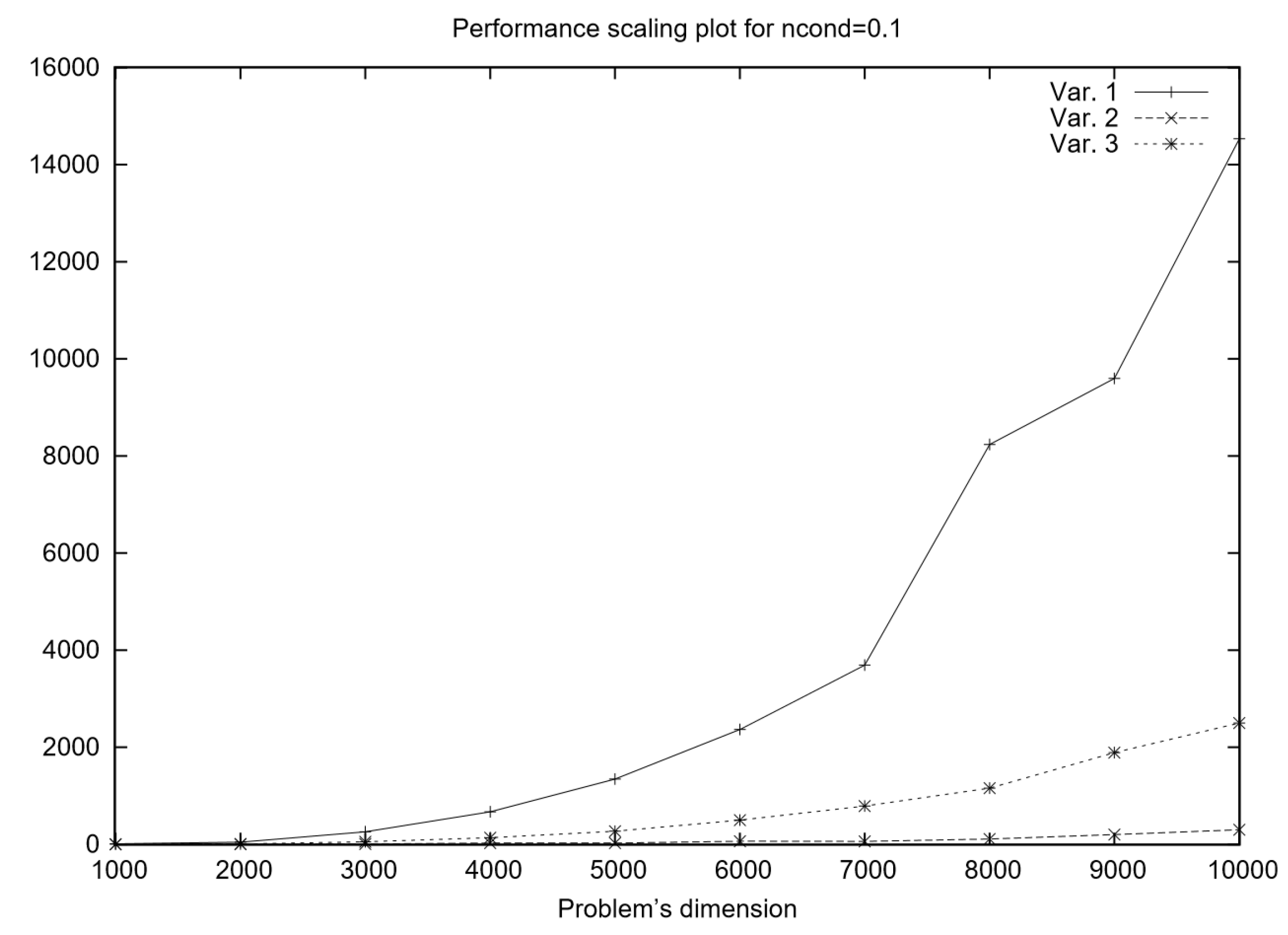
The performance scaling plot in Figure 2 compares the runtime of three algorithmic variants for solving well-conditioned problems, where half of the variables are fixed on bounds. The primary computational task in the algorithm is solving a linear system at each iteration, and the three variants differ in their approach to this task. We can an infer that for small problem sizes, the differences between the three variants are relatively minor. However, as the problem size grows, Variant 1 (${LDL}^T$ decomposition at every iteration) exhibits the steepest runtime increase due to the high cost of repeated factorizations. Meanwhile, Variant 2 (CG throughout) shows much better scalability, with its runtime growing at a slower rate, making it preferable for large-scale problems. Variant 3 (hybrid) likely demonstrates an intermediate performance profile, outperforming Variant 1 in terms of efficiency while maintaining better numerical robustness than Variant 2.

In summary, if computational speed is the primary concern, Variant 2 (CG) is the most scalable option, particularly for large problem sizes. If numerical stability and accuracy are the priority, Variant 1 (${LDL}^T$) is the most robust but at the cost of significantly higher computation time. Variant 3 (hybrid) emerges as an optimal middle-ground approach, balancing efficiency and stability by combining iterative and direct methods. The performance-scaling trends confirm these expectations, with Variant 1 becoming increasingly costly, Variant 2 scaling efficiently, and Variant 3 offering a competitive compromise.

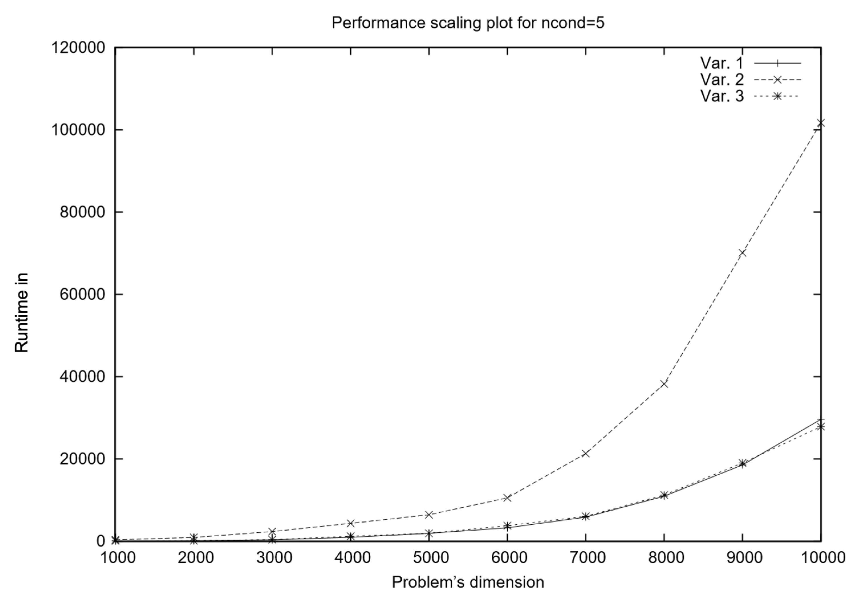
For ill-conditioned problems (see Figure 3, the performance-scaling behavior of the three algorithmic variants shifts significantly compared to well-conditioned problems. In such cases, the system matrix exhibits a high condition number, which impacts both direct and iterative solution methods differently.

From the runtime trends observed in Figure 3 in the new performance scaling plot, it appears that Variant 1 (${LDL}^T$) performs better than in the well-conditioned scenario. This is likely due to the fact that ${LDL}^T$ decomposition, being a direct method, remains robust even when the system matrix is poorly conditioned. Unlike iterative methods, which suffer from slow convergence or numerical instability when the condition number is large, ${LDL}^T$ maintains accuracy at the cost of higher computational effort per iteration. However, in ill-conditioned problems, iterative solvers such as the conjugate gradient (CG) method (used in Variant 2) may require significantly more iterations to converge, making them less efficient overall. This explains why Variant 1, despite its higher theoretical complexity, outperforms the other two methods in this setting.

Variant 3 balances these trade-offs effectively by leveraging the fast initial approximations of CG while maintaining the stability of ${LDL}^T$ in subsequent iterations. While CG may struggle with slow convergence in ill-conditioned problems, using it only in the first iteration can still provide a useful initial guess that reduces the effort needed for ${LDL}^T$ decomposition later on. This reduces the total computational burden of ${LDL}^T$ while still ensuring that subsequent iterations remain numerically stable.

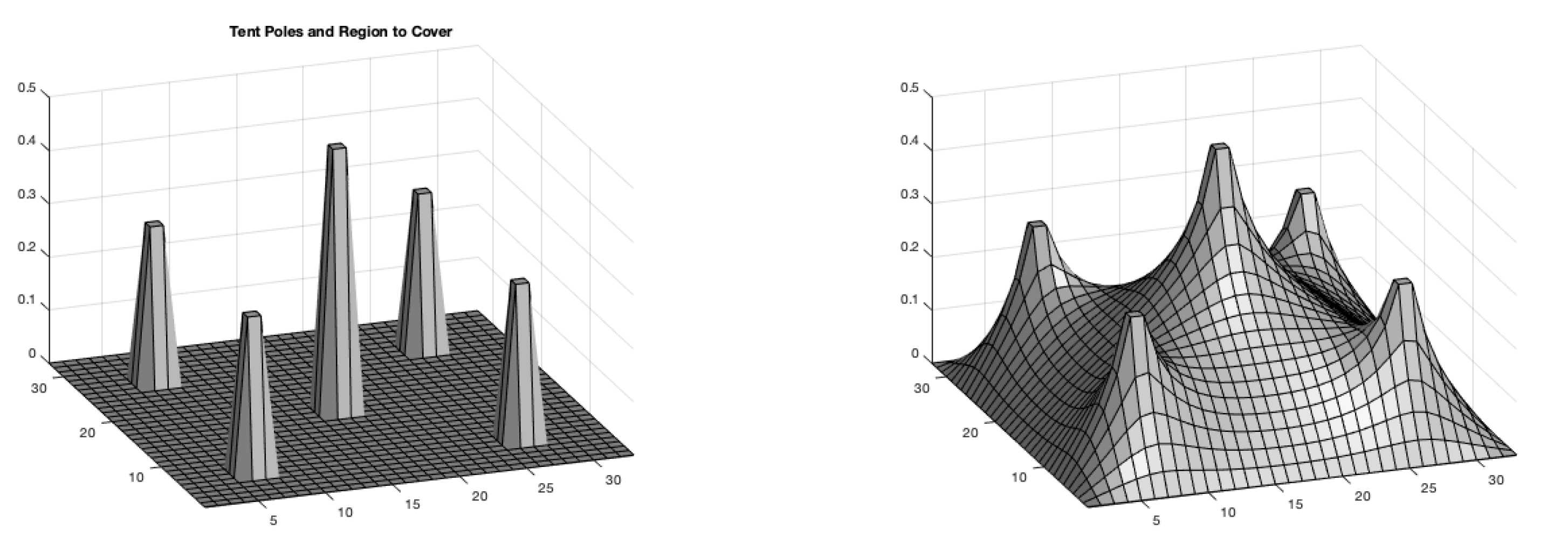
4.2. Circus-Tent Problem

The circus-tent problem serves as a foundational case that highlights how mathematical optimization techniques can be applied to real-world engineering challenges. Its formulation as box-constrained quadratic programming problem is described in detail in Appendix A.2.

Table 6. Results for circus-tent problem case (single-thread execution time in seconds; NC stands for no convergence).

Prob. Name	Var.1	Var.2	Var.3	QN	QPB	QLD	Var.1	Var.2	Var.3	QN	QPB	QLD
Tent (n = 100)	0.01	0.00	0.00	0.00	NC	0.00	5	1	1	1	6	1
Tent (n = 400)	0.32	0.13	0.21	NC	NC	0.25	5	1	2	6	6	3
Tent (n = 900)	5.57	1.45	3.27	NC	NC	2.77	5	1	3	6	6	2
Tent (n = 1600)	48.30	9.57	29.11	NC	NC	20.53	5	1	3	6	6	2
Tent (n = 3600)	557.74	55.74	284.05	NC	NC	246.04	5	1	3	6	6	2
Tent (n = 4900)	1333.51	150.49	696.21	NC	NC	617.58	5	1	3	6	6	2
Average Ranking							5.00	1.00	2.83	6.00	6.00	2.00

presents execution times for different solution approaches to the circus-tent problem across increasing problem sizes, measured in seconds. As the problem size grows, Variant 1 becomes increasingly expensive due to the repeated direct factorization, reaching 1333.51 s for $n=4900$. Variant 2, relying entirely on the iterative CG method, exhibits significantly better scalability, with execution time increasing more gradually to $150.49$ s at $n=4900$. Variant 3, which blends iterative and direct methods, initially performs better than Variant 1 but eventually shows similar growth in execution time, reaching $696.21$ s for the largest problem size. Among the solvers compared, QUACAN successfully solves only the smallest in negligible time but fails for larger cases. QPBOX is unable to solve any instance, as indicated by the NC values across all entries. QLD, however, demonstrates competitive performance, outperforming Variant 1 and Variant 3 for larger problems, reaching $617.58$ s for $n=4900$.

From these results, Variant 2 (conjugate gradient method) proves to be the most efficient and scalable, particularly for larger problem sizes, making it the preferred choice for large-scale computations. Variant 3 (hybrid approach) offers a reasonable compromise between iterative and direct methods, performing well for small-to-medium problems before exhibiting similar computational demands to Variant 1. Variant 1 (${LDL}^T$ decomposition), while accurate, is computationally expensive and less suitable for large-scale applications. Among the solvers, QLD remains the most competitive alternative, performing consistently better than ${LDL}^T$-based methods for larger problem sizes.

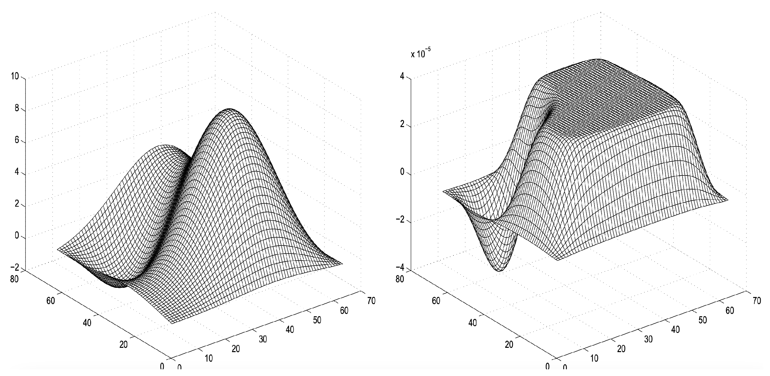
4.3. Biharmonic Equation Problem

The biharmonic equation arises in elasticity theory and describes the small vertical deformations of a thin elastic membrane. In this work, we consider an elastic membrane clamped on a rectangular boundary and subject to a vertical force while being constrained to remain below a given obstacle. This leads to a constrained variational problem that can be formulated as a convex quadratic programming (QP) problem with bound constraints. For more details about the formulation, see Appendix A.3.

Table 7. Results for the biharmonic equation case (single-thread execution time in seconds).

Prob. Name	Var.1	Var.2	Var.3	QN	QPB	QLD	Var.1	Var.2	Var.3	QN	QPB	QLD
Biharm (n = 100)	0.00	0.00	0.00	0.00	0.01	0.01	1	1	1	1	5	5
Biharm (n = 400)	0.20	0.21	0.19	0.65	0.64	0.75	2	3	1	5	4	6
Biharm (n = 900)	4.28	3.13	2.92	18.52	10.49	9.29	3	2	1	6	5	4
Biharm (n = 1600)	23.33	17.89	15.31	119.66	82.12	60.87	3	2	1	6	5	4
Biharm (n = 2500)	106.19	77.24	60.57	775.03	333.91	222.79	3	2	1	6	5	4
Biharm (n = 3600)	308.73	271.46	186.89	2988.08	1071.34	684.57	3	2	1	6	5	4
Biharm (n = 4900)	816.13	705.52	484.45	8282.04	3067.21	1837.66	3	2	1	6	5	4
Average Ranking							2.57	2.00	1.00	5.14	4.86	4.43

presents execution times (in seconds) for different numerical methods applied to the biharmonic equation problem across increasing problem sizes. As the problem size increases, Variant 1 exhibits the steepest growth in execution time, reaching $816.13$ s for the largest case ($n=4900$). Variant 2, which leverages iterative solvers, scales better, achieving a significantly lower execution time of $705.52$ s for the same problem size. Variant 3 strikes a balance between direct and iterative methods, showing better performance than Variant 1 but remaining slightly less efficient than Variant 2, with $484.45$ s for the case $n=4900$.

In the series of solver tests, QLD demonstrates superior performance compared to QUACAN and QPBOX, solving the largest problem in 1837.66 s. By contrast, QUACAN and QPBOX exhibit considerably worse scalability, with times of 8282.04 s and 3067.21 s, respectively, for $n=4900$. QUACAN shows effectiveness with smaller problems but becomes very inefficient as the problem size grows, whereas QPBOX follows a similar pattern, though it performs somewhat better. The findings emphasize that Variant 3 is the most scalable method, making it the optimal choice for large-scale biharmonic problems. Additionally, all BoxCQP variants outperform the competition in this scenario.

4.4. Intensity-Modulated Radiation Therapy

Intensity-Modulated Radiation Therapy (IMRT) is an advanced radiotherapy technique that optimizes the spatial distribution of radiation to maximize tumor control while minimizing damage to surrounding healthy tissues and vital organs. The goal is to deliver a precisely calculated radiation dose that conforms to the tumor shape, reducing side effects and improving treatment effectiveness.

This problem is typically formulated as a quadratic programming (QP) task, where the objective is to determine the optimal fluence intensity profile for a given set of beam configurations. The radiation dose distribution can be represented as a linear combination of beamlet intensities, allowing for a mathematical optimization approach. Given a set of desired dose levels, the optimal beamlet intensities are computed by solving a quadratic objective function that minimizes the difference between the prescribed and delivered doses. The optimization constraints include dose limits for critical organs and physical feasibility conditions. In Appendix A.4, we present in some details the derivation of the formulation.

In practical applications, inverse treatment planning in IMRT requires solving a quadratic optimization problem of the form shown in Equation (9) multiple times, as beam configurations are iteratively adjusted to meet clinical constraints. Since the process involves large-scale quadratic systems, efficient solvers are essential to ensure fast and accurate treatment planning.

$$\begin{array}{c}\hfill {\displaystyle \underset{f}{min}s\left(f\right)=\frac{1}{2}{f}^{T}Af+f^{T}b}\\ \hfill \mathrm{subject}\mathrm{to}f\ge 0\end{array}$$

(9)

Table 8. Results for the Intensity-Modulated Radiation Therapy case (single-thread execution time in seconds).

Prob. Name	Var.1	Var.2	Var.3	QN	QPB	QLD	Var.1	Var.2	Var.3	QN	QPB	QLD
IMRT (n = 2342)	54.22	33.11	40.56	85.11	67.88	73.22	3	1	2	6	4	5
Average Ranking							3.00	1.00	2.00	6.00	4.00	5.00

showcases findings derived from actual data generously shared by S. Breedveld [34]. In this scenario, seven beams are integrated, leading to a quadratic problem comprising 2342 parameters. In this instance, Variants 2 and 3 exhibit superior performance, outperforming their counterparts by a factor of two.

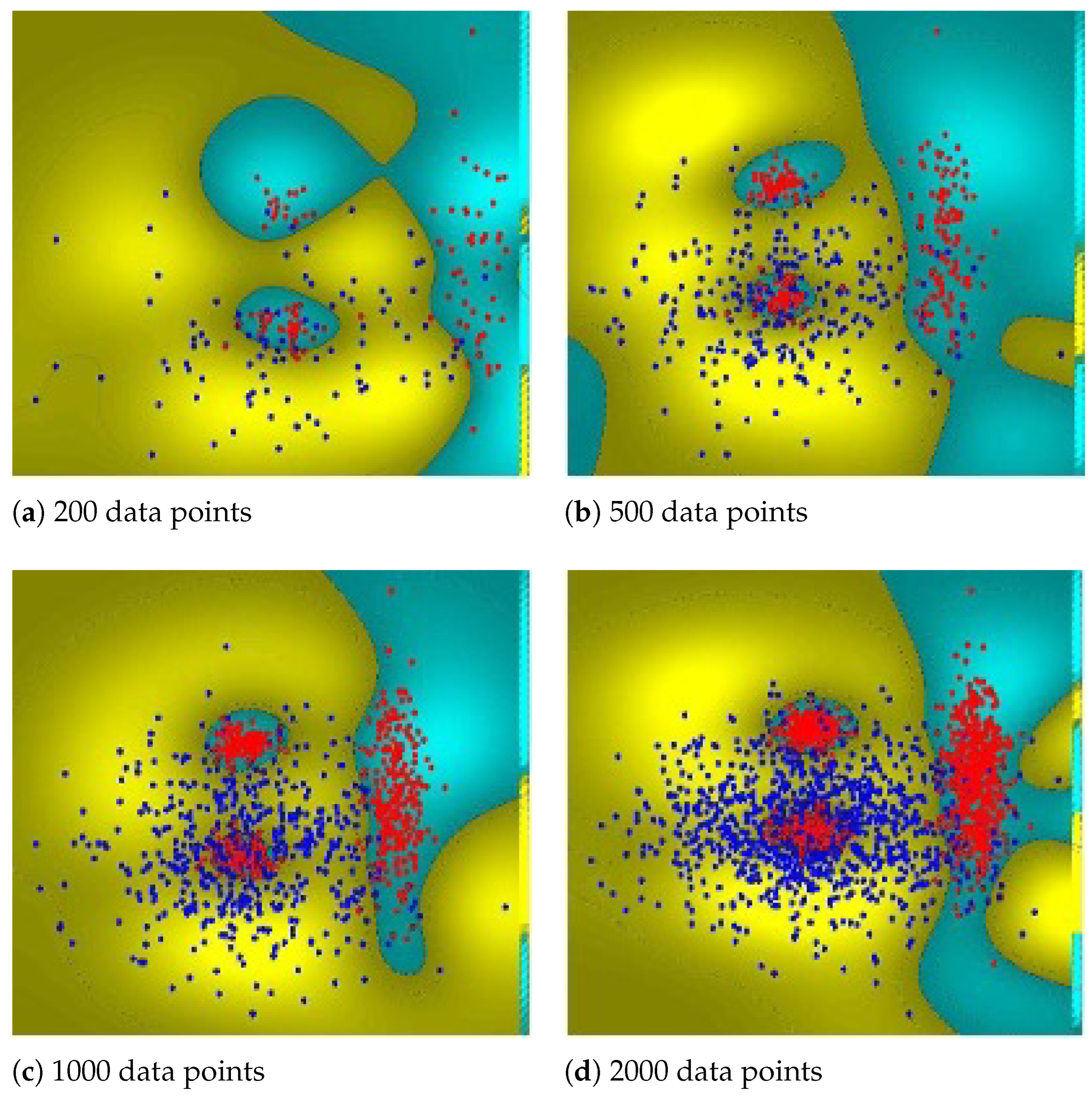
4.5. Support Vector Classification

To create the problem for the case of Support Vector Classification, we used the CLOUDS dataset [35] a well-estabalished two dimensional and two-class classification task. The specifics of the quadratic programming formulation are provided in the Appendix A.5. We run different experiments for an increasing number of CLOUDS datapoints. From

Table 9. Results for SVM training (single-thread execution time in seconds).

Prob. Name	Var.1	Var.2	Var.3	QN	QPB	QLD	Var.1	Var.2	Var.3	QN	QPB	QLD
SVM (n = 100)	0.00	0.00	0.00	0.01	0.01	0.00	1	1	1	5	5	1
SVM (n = 200)	0.04	0.04	0.04	0.15	0.07	0.07	3	1	1	6	4	4
SVM (n = 300)	0.14	0.09	0.10	0.39	0.23	0.25	3	1	2	6	4	5
SVM (n = 400)	0.37	0.29	0.33	2.09	0.53	0.63	3	1	2	6	4	5
SVM (n = 500)	0.70	0.61	0.71	4.69	1.05	1.27	2	1	3	6	4	5
SVM (n = 600)	1.18	0.84	0.97	6.54	1.85	2.36	3	1	2	6	4	5
SVM (n = 700)	2.26	1.51	1.85	14.33	3.03	3.81	3	1	2	6	4	5
SVM (n = 800)	3.38	1.87	2.25	21.75	4.68	6.19	3	1	2	6	4	5
SVM (n = 900)	5.67	3.40	3.84	27.16	7.33	8.20	3	1	2	6	4	5
SVM (n = 1000)	7.26	4.29	5.01	34.01	10.39	11.33	3	1	2	6	4	5
SVM (n = 2000)	68.78	22.01	36.24	256.22	77.29	104.31	3	1	2	6	4	5
SVM (n = 3000)	263.35	63.97	151.40	1068.97	264.56	354.43	3	1	2	6	4	5
Average Ranking							2.75	1.00	1.92	5.92	4.08	4.58

, we can see that Variant 1 experiences significant growth in execution time, reaching $263.35$ s for $n=3000$, making it the least efficient among the three variants. In contrast, Variant 2 scales much better due to its reliance on iterative methods, requiring $63.97$ s for the largest problem. Variant 3, which combines both iterative and direct methods, shows even better performance than Variant 1 for larger problems, reducing execution time to $151.40$ s at. When comparing solver performance, QUACAN, QPBOX, and QLD also display increasing execution times as problem sizes grow. QUACAN shows relatively poor scalability, requiring $1068.97$ s for $n=3000$, making it the slowest solver in the test. QPBOX, while performing better, still struggles with larger problem sizes, reaching $264.56$ s at $n=3000$. QLD, is completing the largest problem in $354.43$ s, yet still significantly slower than Variants 2 and 3. These results highlight that Variant 2 (conjugate gradient method) is the most scalable approach, making it the preferred choice for large-scale SVM problems. Variant 3 (hybrid approach) still offers the best balance between iterative and direct solvers. Therefore, the findings suggest that a combination of CG-based techniques is optimal for solving large-scale SVM optimization problems efficiently.

4.6. Summarizing Fortran Experimental Results

The performance of the six solver variants—Variant 1, Variant 2, Variant 3 versus QUACAN, QPBOX, and QLD—was evaluated across a diverse set of convex quadratic programming problems.

Each case revealed different characteristics of the solver behavior. In the random problem set, Variant 3 and Variant 2 consistently achieved the lowest average rankings ($2.30$ and $2.35$, respectively, on all 90 cases), indicating robust and efficient performance, especially under varying condition numbers. QUACAN followed with an average rank of $3.86$, while QPBOX and QLD were generally slower ($4.40$ and $5.53$, respectively), reflecting their higher computational overheads.

In the context of the biharmonic scenario, characterized by structured sparse problems, Variant 3 emerged as the leader, boasting the top average rank ($1.00$), with Variant 2 not far behind ($2.00$). A similar pattern occurred in the circus-tent problem, where Variant 2 was clearly the standout performer, achieving the highest average rank ($1.00$), while QLD followed in second place ($2.00$), demonstrating its effectiveness for structured geometric problems when feasible. For SVM classification tasks, Variant 2 excelled, with an average rank of $1.00$, and was trailed by Variant 3 and Variant 1. Meanwhile, QLD and QPBOX showed inferior performance, especially with large datasets, due to scaling challenges. In the singular IMRT instance, Variant 2 along with Variant 3 were rated highest, emphasizing their competitiveness even in substantial real-world applications.

In

Table 10. Aggregated results for all cases (average ranking).

Prob. Name	Var.1	Var.2	Var.3	QN	QPB	QLD
Total Average Ranking	3.00	2.33	2.11	3.81	4.44	5.11

we present aggregated ranking results for all the test problem cases. When evaluating all problems together, the aggregate average ranking supports the prior findings. Variant 3 and Variant 2 secured top overall rankings of $2.11$ and $2.33$, respectively, with Var.1 following at $3.00$. Among the other solvers, QUACAN occupied a central rank of $3.81$, while QPBOX and QLD frequently ranked lower at $4.44$ and $5.11$, respectively. These outcomes highlight the robustness and versatility of the proposed BoxCQP variants, particularly Var.2 and Var.3, which effectively balance speed and dependability across diverse problem categories.

5. Experimental Results—Python Implementation

Porting code from Fortran 77 (F77) and MATLAB R2023b to Python 3.8 offers significant advantages in terms of accessibility, reproducibility, and community engagement, making it highly beneficial for exposure in the scientific computing community. Python’s open-source nature, extensive ecosystem, interoperability, and modern programming features make it an ideal platform for sharing, optimizing, and scaling scientific applications. In this section, we present some experimental results from the Python implementation of BoxCQP.

5.1. Linear Least Squares with Bound Constraints

Linear least squares with bound constraints (LLSBC) is a convex optimization problem that bridges classical linear algebra and modern optimization theory. By imposing simple bound constraints to a linear least-squares objective, we obtain a quadratic program (QP) that is guaranteed to be convex.

In practice, adding bound constraints to a least-squares problem is hugely important because it lets us incorporate prior knowledge or physical limitations into the solution. Ordinary linear least squares (OLS) may produce solutions that are mathematically optimal but physically impossible or undesirable (e.g., negative values for inherently non-negative quantities, or parameters outside a feasible range). LLSBC addresses this by enforcing simple “box” constraints (${\ell }_i\le x_i\le u_i$) on the solution vector. This leads to more realistic and interpretable models in many fields. For instance, in machine learning and statistics, it is often unreasonable for certain coefficients to be negative or to exceed certain values (consider probabilities, ages, or concentrations). By constraining coefficients to be non-negative or within a plausible range, we guarantee that the model’s outputs make sense (e.g., predicted prices or counts cannot be negative)

In engineering and the sciences, bound constraints allow us to respect physical laws or design limits—for example, in control systems, we might require gain parameters to remain within stable ranges, or in curve fitting, we might enforce that a response is non-decreasing with an input. In signal processing and image processing, constraints like non-negativity (pixel intensities, power spectra) or monotonicity can significantly improve solutions by reducing noise artifacts and preventing unphysical oscillations. Overall, LLSBC is interesting because it enhances the least-squares approach with robustness and domain knowledge, making the solutions applicable in real-world scenarios where unconstrained solutions would fail. It strikes a useful balance: retaining the computational efficiency and well-understood nature of least squares, while adding just enough constraints to capture practical requirements.

Many regression and estimation tasks in machine learning benefit from bound constraints. A notable example is non-negative least squares (NNLS), where we require $x_i\ge 0$ for all i. This is used when model coefficients represent quantities that cannot go below zero. For instance, when fitting a model to predict prices, ages, or counts, allowing negative coefficients or predictions is not meaningful Imposing non-negativity yields more sensible models and can also have a regularizing effect (often promoting sparsity in the solution similar to an $L_1$ penalty). NNLS is widely used as a subroutine in matrix factorization problems like PARAFAC and non-negative matrix factorization (NMF), where one alternates solving least-squares subproblems under non-negativity constraints. This helps extract interpretable features (e.g., in text mining, image analysis, or clustering) because each factor is constrained to contribute additively (no negative cancellations). Another application is isotonic regression, which is a least-squares problem with a monotonicity constraint ($x_1\le x_2\le \cdots \le x_n$). This can be formulated as LLSBC by introducing linear inequality constraints between variables.

5.2. Problem Definition (Bounded Least Squares)

$$\begin{array}{cc}\hfill & \underset{x\in {\mathbb{R}}^n}{min}{\displaystyle \frac{1}{2}}{\parallel Ax-b\parallel }_2^2,\hfill \\ \hfill & \mathrm{subject}\mathrm{to}{\ell }_i\le x_i\le u_i,i=1,\dots ,n.\hfill \end{array}$$

(10)

where:

• A is an $m\times n$ design matrix;
• b is an m-vector of observations;
• ℓ and u are n-vectors (or scalars) defining lower and upper bounds.

5.3. Expanding the Objective Function

$${\displaystyle \frac{1}{2}}{\parallel Ax-b\parallel }_2^2={\displaystyle \frac{1}{2}}{(Ax-b)}^T(Ax-b).$$

(11)

Expanding this quadratic term:

$${\displaystyle \frac{1}{2}}{(Ax-b)}^T(Ax-b)={\displaystyle \frac{1}{2}}{x}^T{A}^{T}Ax-b^{T}Ax+{\displaystyle \frac{1}{2}}{b}^{T}b.$$

(12)

Ignoring the constant term ${\displaystyle \frac{1}{2}}{b}^{T}b$ (since it does not affect the minimizer), we obtain the standard **convex quadratic program (QP) form**:

$$\underset{x}{min}{\displaystyle \frac{1}{2}}{x}^T\left(A^{T}A\right)x-{\left(A^{T}b\right)}^{T}x,\mathrm{s}.\mathrm{t}.\ell \le x\le u.$$

(13)

5.4. Standard Quadratic Programming Representation

Rewriting the problem in standard QP form:

$$\underset{x}{min}{\displaystyle \frac{1}{2}}{x}^{T}Qx+c^{T}x,\mathrm{subject}\mathrm{to}\ell \le x\le u,$$

(14)

where:

$$\begin{array}{cc}\hfill Q& =A^{T}A(\mathrm{symmetric}\mathrm{positive}\mathrm{semidefinite}\mathrm{matrix}),\hfill \end{array}$$

(15)

$$\begin{array}{cc}\hfill c& =-A^{T}b.\hfill \end{array}$$

(16)

This formulation ensures that the problem is a convex QP since Q is positive semidefinite (or positive definite if A has full column rank).

Experimental Setup

For comparison, we utilize SciPy, a robust open-source Python library for scientific computing and optimization, offering efficient numerical methods for linear algebra, optimization, signal processing, and statistical analysis. Specifically, the scipy.optimize.lsq_linear function is employed to solve bounded linear least-squares problems of the form of Equation (10). The solution is obtained using two distinct approaches: Trust-Region Reflective (TRF) and Bounded Variable Least Squares (BVLS) algorithms.

The TRF (Trust-Region Reflective) algorithm [36] is a subspace trust-region method that is particularly effective for solving large-scale and well-conditioned least-squares problems. It operates by iteratively refining the solution within a trust region, ensuring that the step size remains appropriate to maintain stability. This method enforces bound constraints using an active-set strategy, meaning it considers only variables that are likely to be active at the optimal solution. Trust-region methods are robust, particularly when dealing with ill-conditioned problems, as they naturally handle numerical instabilities and provide controlled step updates.

The BVLS (Bounded Variable Least Squares) algorithm [37] is a projection-based method that explicitly enforces bound constraints at each iteration. Unlike TRF, which works in a trust-region framework, BVLS solves a sequence of unconstrained least-squares problems while ensuring that the solution stays within the prescribed bounds. It follows a gradient-based active-set approach, where variables are either held at their bounds or updated according to the gradient direction, leading to the efficient handling of constraints. This method is particularly useful when strict bound enforcement is crucial, as it prevents overshooting beyond limits at any step.

Our Python implementation is presented in the Appendix A and it directly solves the problem in Equation (14). Notice that we include in timing the multiplications in Equations (15) and (16).

In

Table 11. Linear least-squares random cases (single-thread execution time in seconds).

Prob. Name	Variant 1	lsq_linear-TRF	lsq_linear-BVLS
LSQ (m = 2000, n = 500)	0.02	0.95	0.63
LSQ (m = 2000, n = 1000)	0.12	4.22	2.23
LSQ (m = 2000, n = 1500)	0.21	6.85	12.30
LSQ (m = 2000, n = 2000)	0.45	12.45	25.37
LSQ (m = 20,000, n = 500)	0.00	4.75	3.42
LSQ (m = 20,000, n = 1000)	0.28	18.32	10.94
LSQ (m = 20,000, n = 1500)	0.69	35.12	25.83
LSQ (m = 20,000, n = 2000)	1.26	69.12	49.71

we present execution times (in seconds) for solving random linear least squares (LSQ) problems with bound constraints using three different methods: Variant 1, lsq_linear-TRF, and lsq_linear-BVLS. The problem sizes n vary in terms of the number of observations m. Variant 1 consistently outperforms both lsq_linear-TRF and lsq_linear-BVLS in terms of execution time. For smaller problem sizes, (such as $m=2000$ and $n=500$), Variant 1 completes the computation in $0.02$ s, whereas lsq_linear-TRF and lsq_linear-BVLS require $0.95$ s and $0.63$ s, respectively. As the problem size increases, the execution time of Variant 1 scales more efficiently compared to the other two methods. For example, for dimension ($m=\mathrm{20,000}$, $n=2000$), Variant 1 takes $1.26$ s, whereas lsq_linear-TRF and lsq_linear-BVLS require $69.12$ s and $49.71$ s, respectively. This significant difference highlights the computational efficiency of Variant 1, particularly for large-scale problems.

5.5. 225-Asset Portfolio Optimization Problem

The 225-Asset problem refers to a large-scale quadratic programming formulation used in portfolio optimization, where the objective is to minimize the portfolio’s risk (variance) subject to a set of linear constraints. The problem involves a universe of 225 assets and is based on a classic mean-variance optimization model proposed by Markowitz [38].

Let $x\in {\mathbb{R}}^{225}$ be the portfolio weights vector, where each $x_i$ represents the fraction of the total investment allocated to asset i. The problem is formulated as:

$$\begin{array}{cc}\hfill \underset{x\in {\mathbb{R}}^{225}}{min}& {\displaystyle \frac{1}{2}}{x}^{\top }\Sigma x\hfill \\ \hfill \mathrm{subject}\mathrm{to}& r^{\top }x\ge r_{min}\hfill \\ & {\mathbf{1}}^{\top }x=1\hfill \\ & x\ge 0\hfill \end{array}$$

where

• $\Sigma \in {\mathbb{R}}^{225\times 225}$ is the positive definite covariance matrix of asset returns.
• $r\in {\mathbb{R}}^{225}$ is the expected return vector.
• $r_{min}\in \mathbb{R}$ is the minimum required portfolio return.
• $\mathbf{1}\in {\mathbb{R}}^{225}$ is the vector of ones (to enforce full investment).

The constraints ensure:

• A minimum return threshold is met ($r^{\top }x\ge r_{min}$).
• The portfolio is fully invested (${\mathbf{1}}^{\top }x=1$).
• No short selling is allowed ($x_i\ge 0\forall i$).

This problem is often used as a benchmark in quadratic programming solvers because of its size (225 variables and several hundred constraints) and its relevance in financial optimization. It tests a solver’s ability to handle large, sparse quadratic programs with both inequality and equality constraints in practical applications. To express this problem in the standard quadratic programming form with inequality constraints of the form seen in Equation (2), we perform the following transformations:

• Set $B=\Sigma$, and $d=0$. There is no linear cost term in the mean-variance objective, only the quadratic risk term.
• Encode the return constraint $r^{\top }x\ge r_{min}$ as one row in A and b:
  $A_1=r^{\top }$, $b_1=r_{min}$
• Convert the equality constraint ${\mathbf{1}}^{\top }x=1$ into two inequalities:
  ${\mathbf{1}}^{\top }x\ge 1$ and $-{\mathbf{1}}^{\top }x\ge -1$. These become rows in A:
  $A_2={\mathbf{1}}^{\top }$, $b_2=1$;
  $A_3=-{\mathbf{1}}^{\top }$, $b_3=-1$
• Express the no short-selling constraint $x\ge 0$ as $A_4=I$, the identity matrix, and $b_4=0$

Putting all constraints together:

$$A=\left[\begin{array}{c}{r}^{\top }\\ {\mathbf{1}}^{\top }\\ -{\mathbf{1}}^{\top }\\ I\end{array}\right],b=\left[\begin{array}{c}{r}_{min}\\ 1\\ -1\\ 0\end{array}\right]$$

This formulation is now fully compatible with solvers that accept inequality-only quadratic programs, such as those in the form of Equation (2).

To benchmark the Python implementation of BoxCQP, we compared its performance against two well-established quadratic programming solvers available through the qpsolvers Python interface: quadprog and osqp [39,40]. The quadprog solver is based on the Goldfarb–Idnani active-set method, which is particularly suitable for small- to medium-scale convex QP problems with dense Hessians. In contrast, osqp (Operator Splitting Quadratic Program) is a modern, operator-splitting-based solver that handles large-scale problems efficiently, even when the matrices involved are sparse or poorly conditioned. In

Table 12. 225-Asset portfolio optimization (single-thread execution time in seconds).

Prob. Name	Variant 1	quadprog	osqp
225-Asset (m = 453, n = 225)	0.0062	0.0421	0.0091

, we present some preliminary results comparing BoxCQP to modern antagonistic methods.

5.6. Bound-Constrained Non-Linear Optimization

We introduce a trust-region method for non-linear optimization with bound constraints, where the trust region is defined as a hyperbox, differing from the conventional hypersphere or hyperellipsoid approaches. The rectangular trust region is particularly well suited for problems with bound constraints, as it maintains its geometric structure even when intersecting the feasible region.

Trust-region methods fall in the category of sequential quadratic programming [41,42]. These algorithms are iterative and the objective function $f\left(x\right)$ (assumed to be twice continuously differentiable) is approximated in a proper neighborhood of the current iterate (the trust region), using a quadratic model. Namely, at the $k^{th}$ iteration, the model is given by:

$$f(x^k+s)\approx m^{\left(k\right)}\left(s\right)=f\left(x^{\left(k\right)}\right)+s^T{g}^{\left(k\right)}+{\displaystyle \frac{1}{2}}{s}^T{B}^{\left(k\right)}s$$

(17)

where $g^{\left(k\right)}=\nabla f\left(x^{\left(k\right)}\right)$ and $B^{\left(k\right)}$, in the case of Newton’s method, is a positive definite modification of the Hessian, while in the case of quasi-Newton methods, it is a positive definite matrix produced by the relevant update.

The trust region may be defined by:

$${\mathbf{T}}^{\left(k\right)}=\{x\in {\Re }^n\left|\right||x-x^{\left(k\right)}\left|\right|\le {\Delta }^{\left(k\right)}\}$$

(18)

It is obvious that different choices for the norm lead to different trust-region shapes. The Euclidean norm ${\left|\right|·\left|\right|}_2$ corresponds to a hypersphere, while the ${\left|\right|·\left|\right|}_{\infty }$ norm defines a hyperbox.

Given the model and the trust region, we seek a step $\left|\right|s^{\left(k\right)}\left|\right|\le {\Delta }^{\left(k\right)}$ that minimizes $m^{\left(k\right)}\left(s\right)$. We compare the actual reduction $\delta f^{\left(k\right)}=f\left(x^{\left(k\right)}\right)-f(x^{\left(k\right)}+s^{\left(k\right)})$ to the model reduction $\delta m^{\left(k\right)}=m^{\left(k\right)}\left(0\right)-m^{\left(k\right)}\left(s^{\left(k\right)}\right)$. If they agree to a certain extend, the step is accepted and the trust region is either expanded or remains the same. Otherwise, the step is rejected and the trust region is contracted. The basic trust-region algorithm is sketched in Algorithm 2.

Algorithm 2 Basic trust region

1. Pick the initial point and trust-region parameter $x^{\left(0\right)}$ and ${\Delta }^{\left(0\right)}$, and set $k=0$. 2. Construct a quadratic model: $$f(x^k+s)\approx m^{\left(k\right)}\left(s\right)=f\left(x^{\left(k\right)}\right)+s^T{g}^{\left(k\right)}+{\displaystyle \frac{1}{2}}{s}^T{B}^{\left(k\right)}s$$ 3. Minimize $m^{\left(k\right)}\left(s\right)$ and hence determine $\left|\right|s^{\left(k\right)}\left|\right|\le {\Delta }^{\left(k\right)}$ 4. Compute the ratio of actual to expected reduction: $r^{\left(k\right)}={\displaystyle \frac{\delta f^{\left(k\right)}}{\delta m^{\left(k\right)}}}$, and update the trust region, following the strategy of Dennis and Schnabel [43] (Appendix A, page 338). 5. Increment $k\leftarrow k+1$ and repeat from 1.

Consider the bound-constrained problem:

$$\underset{x}{min}f\left(x\right),\mathrm{subject}\mathrm{to}\text{:}{l}_i\le x_i\le u_i$$

The  unconstrained case is obtained by letting $u_i=-l_i\to \infty$.

Let $x^{\left(k\right)}$ be the k-th iterate of the trust-region algorithm.

Hence, step 3 of Algorithm 2 becomes:

$$\begin{array}{c}\hfill {\displaystyle \underset{s}{min}}{m}^{\left(k\right)}\left(s\right)=s^T{g}^{\left(k\right)}+{\displaystyle \frac{1}{2}}{s}^T{B}^{\left(k\right)}s\hfill \\ \hfill \mathrm{subject}\mathrm{to}\text{:}max(l_i-x_i^{\left(k\right)},-{\Delta }^{\left(k\right)})\le s_i\le min(u_i-x_i^{\left(k\right)},{\Delta }^{\left(k\right)})\hfill \end{array}$$

(19)

We have developed a hybrid trust-region algorithm that utilizes the Hessian matrix to determine the appropriate optimization approach. When the Hessian is positive definite, the algorithm transitions to solving the quadratic subproblem (see Equation (20)). However, if the Hessian is indefinite, we employ the classical method described in [41] to ensure stability and convergence. It is important to note that in the vicinity of a local minimum, the Hessian matrix is typically positive definite, reinforcing the effectiveness of this approach. The complete implementation of the algorithm is provided in Appendix A Listing A3: Python TrustBox Implementation. Preliminary results with random settings (bounded and unbounded) of the well known Rosenbrock function

$$f\left(x\right)=\sum _{i=1}^{n-1}\left[100{(x_{i+1}-x_i^2)}^2+{(1-x_i)}^2\right],\mathrm{with}\mathrm{minimum}\mathrm{at}{x}^{\ast }={[1,1,\dots ,1]}^T.$$

showed us that (a) half of the iterations are positive definite and (b) we achieve a $5\%$ reduction in the total number of iterations.

6. Conclusions

We have presented an active-set algorithm for solving bound-constrained convex quadratic problems, leveraging an approach that dynamically updates both the primal and dual variables at each iteration. The algorithm efficiently determines the active set, allowing for systematic modifications that guide the solution toward feasibility and optimality while maintaining computational efficiency. This approach ensures robust convergence properties and significantly improves the solver’s performance, particularly in handling large-scale problems where traditional quadratic programming methods may struggle.

Extensive experimental testing has demonstrated the superior performance of our approach compared to several well-established quadratic programming solvers. Across a variety of problem sizes and structures, the proposed algorithm exhibited faster execution times, improved numerical stability, and enhanced scalability, making it a compelling alternative for applications requiring bound-constrained optimization. The method performed particularly well in large-scale settings, where efficiently handling constraints is crucial for reducing computational overhead.

Additionally, a trust-region method for non-linear objective functions has emerged as a natural extension of our active-set framework. By integrating the proposed algorithm into the subproblem solver, the trust-region approach is capable of efficiently handling both unconstrained and bound-constrained optimization problems. The flexibility of this integration allows for enhanced adaptability in solving non-linear problems where traditional approaches may fail due to instability or attain a slow convergence.