Article

Harmonizer: A Universal Signal Tokenization Framework for Multimodal Large Language Models

1
Department of Computer Science and Engineering, University of Tennessee at Chattanooga (UTC), 615 McCallie Ave, Chattanooga, TN 37377, USA
2
Department of Electrical and Computer Engineering, Northwestern University, 633 Clark Street, Evanston, IL 60208, USA
3
Feinberg School of Medicine, Division of Cardiac Surgery, Northwestern University, 633 Clark Street, Evanston, IL 60208, USA
4
Center for Artificial Intelligence, Bluhm Cardiovascular Institute, Northwestern Medicine, 633 Clark Street, Evanston, IL 60208, USA
*
Author to whom correspondence should be addressed.
Mathematics 2025, 13(11), 1819; https://doi.org/10.3390/math13111819
Submission received: 27 March 2025 / Revised: 23 May 2025 / Accepted: 25 May 2025 / Published: 29 May 2025

Abstract

:
This paper introduces Harmonizer, a universal framework designed for tokenizing heterogeneous input signals, including text, audio, and video, to enable seamless integration into multimodal large language models (LLMs). Harmonizer employs a unified approach to convert diverse, non-linguistic signals into discrete tokens via its FusionQuantizer architecture, built on FluxFormer, to efficiently capture essential signal features while minimizing complexity. We enhance features through STFT-based spectral decomposition, Hilbert transform analytic signal extraction, and SCLAHE spectrogram contrast optimization, and train using a composite loss function to produce reliable embeddings and construct a robust vector vocabulary. Experimental validation on music datasets such as E-GMD v1.0.0, Maestro v3.0.0, and GTZAN demonstrates high fidelity across 288 s of vocal signals (MSE = 0.0037, CC = 0.9282, Cosine Sim. = 0.9278, DTW = 12.12, MFCC Sim. = 0.9997, Spectral Conv. = 0.2485). Preliminary tests on text reconstruction and UCF-101 video clips further confirm Harmonizer’s applicability across discrete and spatiotemporal modalities. Rooted in the universality of wave phenomena and Fourier theory, Harmonizer offers a physics-inspired, modality-agnostic fusion mechanism via wave superposition and interference principles. In summary, Harmonizer integrates natural language processing and signal processing into a coherent tokenization paradigm for efficient, interpretable multimodal learning.

1. Introduction

Large language models (LLMs) have successfully processed natural language [1,2,3,4], but integrating multimodal inputs requires robust tokenization strategies [5,6,7]. However, existing approaches struggle to align modalities such as text, audio, video, and sensor data into a coherent format that LLMs can effectively process [8]. As a remedy, this paper proposes Harmonizer, a universal signal tokenization framework that enables seamless tokenization of diverse input signals for multimodal LLMs. Employing a unified tokenization strategy ensures a consistent and efficient representation of multimodal data [9,10,11], thus enhancing the adaptability and scalability of LLMs across various domains and applications [12,13,14].
The implementation of Harmonizer faces several critical technical challenges. First, it must address the heterogeneity of input signals, handling differences in representation (e.g., audio waveforms versus image pixels) [15,16]. Second, temporal and spatial resolution pose challenges as sequences often vary in length and resolution [17]. Third, scalability is essential to maintain efficiency as both the number of modalities and the complexity of data increase [18,19]. Finally, preserving contextual semantics ensures accurate integration of cross-modal information (e.g., audio-text alignment) for coherent multimodal reasoning and inference [20]. In NLP, tokenization splits text into small units (words or subwords) and maps them to numbers that capture syntax and meaning [21]. In NLP, tokenization involves breaking text into smaller units (e.g., words or subwords) [22,23] and mapping them to numerical representations using a predefined vocabulary that captures the syntactic and semantic essence of the language [24]. These standardized representations enable LLMs to learn contextual relationships and nuances [25,26]. (In subsequent mentions, we refer to large language models (LLMs) and natural language processing (NLP) only by their abbreviations).
However, applying these well-established principles to signal processing introduces a different set of challenges [27]. Unlike textual data, which inherently consist of discrete units that can be directly mapped to tokens, signals, such as audio, radio, medical, or sensor data, do not naturally possess a vocabulary [28]. Signals are continuous, time-varying data forms composed of an infinite range of values over time or frequency [29], representing physical quantities such as sound pressure, electromagnetic fields, or electrical activity [30]. Consequently, there is no direct equivalent to a “word” or “sentence” in signal data, making traditional NLP tokenization techniques unsuitable [31]. This absence of an intrinsic vocabulary creates a critical gap that requires an innovative approach to effective signal representation [32,33,34,35]. At its core, Harmonizer is grounded in fundamental wave-based principles. Continuous signals—be they acoustic, electromagnetic, or sensor readings [36,37,38,39,40,41]—encode information via smooth variations in amplitude, frequency, and phase [42,43,44]. Fourier analysis guarantees any such signal admits a complete sinusoidal decomposition, furnishing a universal feature basis [45]. Critically, wave superposition and interference allow multiple streams to combine instantaneously and losslessly—no hand-crafted alignment is required—paving the way for robust, real-time fusion across modalities [46,47,48,49]. By leveraging these natural properties, our framework unifies preprocessing, quantization, and tokenization under a single, physically motivated paradigm.
Previous works in signal processing and NLP have laid the foundation for this study. Early research in quantization, such as the Lloyd–Max quantization algorithm [50], established efficient scalar quantization by minimizing the mean squared error between original and quantized signals [51,52]. Later, vector quantization techniques exploited correlations within signal data to produce compact and representative encodings [53,54]. In parallel, NLP saw the emergence of effective tokenization methods, including subword tokenization [5] and byte-pair encoding (BPE) [55] that decompose words into smaller units to improve model generalization [7,56].
To bridge the gap between continuous signal data and the discrete token representations required by machine learning models, we leverage advanced vector quantization techniques to create a meaningful vocabulary for signals [57]. Analogous feature-space augmentation and self-supervised loss strategies—exemplified by PatchUp within a metric-learning framework—have proven to substantially improve embedding diversity and generalization, and can be directly applied to enrich the tokenization of continuous modalities such as audio and video signals [58,59]. At its core, the model employs a quantization vector that compresses signals while preserving essential characteristics and integrates them into a FusionQuantizer architecture built on a FluxFormer-like backbone [60,61]. In addition, advanced preprocessing techniques, including Short-Time Fourier Transform (STFT) [62], Hilbert Transform [63], and Spectrogram Contrast Limited Adaptive Histogram Equalization (SCLAHE) [64], are used to extract rich and nuanced representations from signals. An innovative multi-objective loss function further optimizes the quality of the generated embedding vectors, ensuring that the input data are effectively represented [65,66].
The exponential growth of signal data in fields such as telecommunications, medical diagnostics, multimedia applications, and the Internet of Things (IoT) has driven the need for more efficient methods of signal representation, compression, and analysis [67,68]. Traditional approaches often depend on domain-specific knowledge and lack standardized methodologies for tokenizing signals [69,70], highlighting a critical gap [17]. Addressing this gap requires new frameworks that bridge signal processing and machine learning to enable more universal and efficient representation techniques [71,72,73].
Recent advancements in transformer architectures have significantly improved the processing of multimodal data [74]. Models like Perceiver and Perceiver IO demonstrate the ability to handle various input types, including images, audio, and point clouds, using a unified attention mechanism [75,76]. These models employ latent bottleneck attention to efficiently process high-dimensional data, a technique that has inspired frameworks like Harmonizer to develop modality-agnostic tokenization strategies [77]. Such strategies are crucial for converting diverse input signals into coherent token sequences suitable for large language models (LLMs) [14,78]. In self-supervised learning, models such as wav2vec 2.0 show that pre-training on raw audio can yield robust speech representations without labeled data [79,80]. Likewise, BEiT applies masked image modeling to train vision transformers through the reconstruction of masked patches [81]. These examples highlight the potential of tokenization schemes that align well with unsupervised and pretext tasks in different modalities [82].
Contrastive learning further increases the effectiveness of multimodal tokenization [83]. CLIP, for example, uses a contrastive objective to align the image and text embeddings, enabling a better cross-modal understanding [84,85]. Integrating such techniques into tokenization frameworks ensures that generated tokens are both syntactically consistent and semantically informative, which improves the model’s ability to relate information across modalities [83,86]. Moreover, models like VATT show that learning from raw video, audio, and text data is possible using convolution-free transformers [87]. These models rely on multimodal contrastive loss functions to extract meaningful representations for downstream tasks [88,89]. Unified processing through consistent multimodal tokenization is the key to achieving this level of performance [90]. The evolution of these models underscores the central role of robust tokenization in multimodal learning [90,91]. Using such innovations, frameworks like Harmonizer can generate more efficient, generalizable, and semantically rich representations, improving adaptability across applications [92].
Transformer-based multimodal models, such as the multimodal transformer and the joint multimodal transformer, further illustrate the power of unified attention mechanisms [93,94]. These architectures often use modality-specific encoders followed by cross-modal attention layers to model complex relationships between inputs [95]. This approach proves especially useful in emotion recognition and sentiment analysis, where the fusion of text, audio, and visual cues is essential [96]. Innovations like dual-level feature restoration, as implemented in the Efficient Multimodal Transformer, enhance the tokenization process by preserving fine-grained details, leading to better performance in complex tasks [91,97]. Self-supervised learning (SSL) has emerged as a powerful method to extract representations from unlabeled multimodal data [98,99]. Frameworks like Self-Supervised MultiModal Versatile Networks (MMVs) and Modality-Agnostic Transformer-based Self-Supervised Learning (MATS2L) show how tokenization approaches tailored for SSL can capture both modality-specific and cross-modal features [100,101]. These systems utilize tasks such as masked token prediction and contrastive learning to develop meaningful token representations [102].
In medical imaging, self-supervised multimodal tokenization has enabled the extraction of high-quality features from MRI and CT data, thus improving diagnostics [103,104]. In remote sensing, SSL-based tokenization frameworks have helped integrate satellite data from different sensors, improving land cover classification [105]. Together, the synergy between tokenization strategies, transformer models, and self-supervised objectives continues to redefine the landscape of multimodal learning [98,105]. These developments lay a strong foundation for universal frameworks like Harmonizer, capable of handling various input types efficiently and meaningfully [106,107].
This paper makes the following contributions:
  • Universal Tokenization Framework: We introduce Harmonizer, the first data-driven vocabulary approach that seamlessly tokenizes text, audio, video, and sensor inputs for LLMs.
  • FusionQuantizer and Streaming FluxFormer: We design a novel FusionQuantizer architecture atop a streaming FluxFormer backbone, combining STFT, Hilbert, and SCLAHE preprocessing with hybrid vector quantization for robust, low-latency inference.
  • Multi-Objective Training: We formulate and balance adversarial, time-domain, spectral, and perceptual loss terms, ensuring high fidelity across modalities and dynamic ranges.
  • Cross-Domain Validation: We demonstrate Harmonizer’s versatility through extensive music evaluations (E-GMD, Maestro, GTZAN) and preliminary text (ASCII encoding, one and two words) and video (UCF-101) experiments.
In summary, our proposed approach offers a groundbreaking solution for applying NLP-inspired tokenization techniques to signal processing [29,108,109]. By creating a representative vocabulary for signals and employing a robust quantization vector approach, it enables efficient signal representation and manipulation, paving the way for future advancements in both signal processing and machine learning.

2. Overview of Harmonizer

LLMs have successfully processed natural language [1,2,3,4], but integrating multimodal inputs requires robust tokenization strategies [5,6,7]. However, existing approaches struggle to align modalities such as text, audio, video, and sensor data into a coherent format that LLMs can effectively process [8,110]. As a remedy, this paper proposes Harmonizer, a universal signal tokenization framework that enables seamless tokenization of diverse input signals for Multimoda Large Language Models (MLLMs). Employing a unified tokenization strategy ensures consistent and efficient representation of multimodal data, thereby enhancing the adaptability and scalability of MLLMs across various domains and applications.
The deployment of Harmonizer encounters several significant technical obstacles. Primarily, it must manage the heterogeneity of input signals by accommodating varying representations (e.g., audio waveforms versus image pixels) [15,16]. Additionally, temporal and spatial resolution differences present challenges since sequences frequently differ in length and clarity [17]. Furthermore, scalability is critical to ensure efficiency as both the number of modalities and the complexity of the data expand [18,19]. Finally, it is essential to preserve contextual semantics, ensuring contextual information is accurately retained and integrated between diverse data types to facilitate seamless interaction [20].
  • Tokenization via Quantization and Vocabulary Generation:
  • Signal Quantization: Harmonizer introduces a unique approach to signal processing by creating a quantization vector that serves as the basis for developing a signal vocabulary. This dynamic quantization technique transforms the continuous signal space into a finite set of discrete levels, thereby reducing the signal data size while preserving its essential features [50,51,57,111,112].
  • Signal Tokenization: Building upon the quantization process, the framework creates a vocabulary of tokens representing different signal segments. Each token corresponds to a specific quantized level, much like how words are tokenized in NLP [22,23,113,114]. This structured tokenization enables machine learning models to interpret signals effectively.

2.1. Creating a Vocabulary for Signals

One of the most challenging aspects of applying NLP techniques to signals is the absence of a predefined vocabulary. Harmonizer addresses this using a data-driven approach to generate a vocabulary that captures the unique characteristics of the signal. The process involves the following steps:
  • Feature Extraction: Initially, relevant features are extracted from the signals (e.g., amplitude, frequency, and phase in the case of audio signals) [30,115,116].
  • Clustering: Unsupervised learning techniques are then used to group similar features, identifying patterns and repetitive elements within the signal data [52,117,118,119].
  • Token Generation: Each resulting cluster is assigned a unique token, forming the basis of the signal vocabulary. This process is iterative, refining the vocabulary over time to enhance accuracy and representation [120].

2.2. Signal Compression via Quantization Vector Techniques

Signal compression is critical for optimizing storage and transmission. Harmonizer leverages quantization vector techniques to encode high-dimensional signal data into a lower-dimensional form without significant loss of information [57,121,122]. By mapping complex signal data to a compact quantization vector, the framework achieves efficient compression while retaining the integrity and essential characteristics of the original signal. This compression methodology is particularly advantageous in scenarios where bandwidth is limited or storage capacity is constrained ( e.g., in medical imaging applications, where high-resolution images need to be stored and transmitted without compromising diagnostic quality) [36].

3. Implementation Methodology of Harmonizer

Harmonizer is designed as a universal tokenization framework that unifies the treatment of diverse input signals (e.g., audio, sensor data, text, video) for MLLMs. Figure 1 provides an overview of the Harmonizer architecture, illustrating its core components and the data flow from raw signal inputs to final tokenized outputs and reconstructed signal. The Division Unit in Figure 1 is in charge of data preparation. This unit can handle both continuous and discrete tokens; if the input is analog, the inputs are sampled into discrete-time signals before processing. The input is divided into chunks if it is a signal. Textual input is first transformed into a signal by combining a sine function with ASCII encoding. Video input is converted into a signal format by extracting and concatenating spatiotemporal patches.

3.1. Preprocessing and Feature Extraction

Harmonizer begins with domain-specific preprocessing steps that convert raw inputs, such as audio waveforms or sensor data streams, into feature representations suitable for quantization. For audio and other time-varying signals, the STFT is computed to capture local frequency content and detect transients and harmonics. The Hilbert Transform is applied to extract analytic signal properties, including instantaneous amplitude and phase, facilitating precise modeling of nonstationary data. The SCLAHE algorithm enhances local contrast in spectrograms, making subtle features more distinguishable. These modular operations convert raw data into high-resolution spectral or time-frequency representations that capture critical nuances before tokenization.

3.2. Fluxhead-Based Fusion Quantizer Unit

The core of Harmonizer is the FusionQuantizer, which extends our FluxHead and FluxFormer modules to learn a compact codebook of signal patterns. In the feature encoding stage, FluxHead and 1D Convolutional layers ingest preprocessed feature maps and leverage a streaming multi-head self-attention mechanism to integrate both temporal and spectral cues, ensuring that local patterns and global context are captured. FluxHead starts processing immediately on the first incoming frame, so the model can handle inputs of any length with minimal delay. The encoded features are then quantized into discrete tokens through a data-driven vector quantization process that learns a signal vocabulary representing diverse signal patterns such as partials, formants, and onsets. For multimodal data (e.g., audio combined with text), a cross-attention fusion mechanism aligns and unifies tokens across modalities, enabling seamless integration with downstream large language models.

3.3. Streaming Inference and LLM Integration

Once trained, Harmonizer operates in a streaming fashion. Incoming signals, whether audio frames, text chunks, or sensor batches, are processed in small segments via a sliding window, enabling near real-time token generation. Each segment is passed through the FluxHead and FluxFormer-based pipeline to produce tokens on the fly with minimal latency. These tokens are subsequently fed into or combined with large language models, allowing for context-aware, multimodal reasoning or generation without requiring complete input sequences. This design readily supports integration into Retrieval-Augmented Generation (RAG) systems and other knowledge-intensive workflows by unifying heterogeneous signals into a coherent token space.

3.4. Mathematical Formulation of Harmonizer with Attention Mechanism

3.4.1. Input Audio Signal Representation

An audio signal is represented as a multi-dimensional tensor:
x real R B × C × T ,
where B is the batch size, C is the number of channels, and T is the number of time steps. This tensor serves as the input to the model.

3.4.2. Encoding via Convolutional Layers

The encoder begins with convolutional layers for feature extraction. For each convolutional layer i, the output is computed as
z ( i ) = σ W ( i ) x ( i ) + b ( i ) ,
where W ( i ) R F ( i ) × C × K ( i ) is the convolutional filter, F ( i ) is the number of feature maps, K ( i ) is the kernel size, b ( i ) is the bias term, σ denotes the ReLU activation function, and ∗ represents convolution. Let
z ( l conv ) R B × F ( l conv ) × T ( l conv )
denote the final output after the last convolutional layer.

3.4.3. FluxHead: Streaming Multihead Attention Encoder

The convolutional features z ( l conv ) are then processed by the FluxHead module. First, a positional encoding is added as follows:
z pos = z ( l conv ) + P ,
where P R T × d is a positional encoding that can be computed using sinusoidal functions as follows:
P ( m , 2 n ) = sin m 10,000 2 n d , P ( m , 2 n + 1 ) = cos m 10,000 2 n + 1 d
with m as the position index and n as the dimension index.
  • For each attention head j ( 1 j h ), the projections are computed as
Q j = W Q j z pos , K j = W K j z pos , V j = W V j z pos ,
with learned matrices W Q j , W K j , and W V j . The attention weights are given by
A j = softmax Q j ( K j ) d h ,
where d h = d / h . The head outputs are then
head j = A j V j .
  • All head outputs are concatenated and projected as follows:
z ˜ ( A H ) = Concat head 1 , , head h W O ,
with W O as the output projection matrix. This attention-refined representation  z ˜ ( A H ) is passed to the quantization stage.

3.4.4. FusionQuantizer

Within the FusionQuantizer module, the attention-refined features z ˜ ( A H ) are quantized using a hybrid approach that combines residual and hierarchical quantization techniques. This design choice is motivated by two main factors:
  • Residual Quantization: This method iteratively minimizes the quantization error by first approximating the input with a coarsely quantized code and then quantizing the residual (i.e., the difference between the input and its approximation). By doing so, it preserves fine-grained details that might otherwise be lost if only a single quantization step were applied.
  • Hierarchical Quantization: In parallel, hierarchical quantization captures the data’s multi-scale semantic structure. It organizes the quantization process into several levels, enabling the model to extract both coarse (global) and fine (local) features from the input. This multi-level approach is especially useful for complex data representations.
By fusing the outputs of these two methods, the model benefits from both the refined approximation of residual quantization and the robust, multi-scale representation of hierarchical quantization. This fusion results in a latent representation that effectively balances representational fidelity with compactness, ultimately enhancing the model’s performance on downstream tasks.
In the first-level quantization, vocabulary codebooks C ( 1 R ) and C ( 1 H ) are defined as
c ^ ( 1 R ) = arg min c i ( 1 R ) C ( 1 R ) z ˜ ( A H ) c i ( 1 R ) 2 2 ,
c ^ ( 1 H ) = arg min c i ( 1 H ) C ( 1 H ) z ˜ ( A H ) c i ( 1 H ) 2 2 .
A residual is computed as
r ( 1 R ) = z ˜ ( A H ) c ^ ( 1 R ) ,
which is then quantized using a second-level codebook C ( 2 R ) :
c ^ ( 2 R ) = arg min c i ( 2 R ) C ( 2 R ) r ( 1 R ) c i ( 2 R ) 2 2 .
Hierarchical quantization operates directly on the attention-refined features to capture multi-scale semantic information:
c ^ ( 2 H ) = arg min c i ( 2 H ) C ( 2 H ) z ˜ ( A H ) c i ( 2 H ) 2 2 .
The final quantized latent representation is obtained by fusing the outputs from both quantization strategies:
z ^ = 1 2 c ^ ( 1 R ) + c ^ ( 1 H ) + c ^ ( 2 R ) + c ^ ( 2 H ) + + c ^ ( L R ) + c ^ ( L H ) .
While the mathematical form above fuses residual and hierarchical codebook outputs, the underlying idea is straightforward. Residual quantization iteratively captures the fine-grained differences left over after a coarse approximation, ensuring precise reconstruction of subtle signal details. Hierarchical quantization, in contrast, targets multi-scale structure by first encoding broad, global patterns and then refining them at finer levels. By averaging these two perspectives, the FusionQuantizer benefits from both the accuracy of residual error minimization and the robustness of multi-level feature capture. This balanced fusion yields a compact yet expressive latent representation that faithfully preserves both coarse structure and fine details. This fusion ensures that the latent representation benefits from the iterative error minimization of residual quantization as well as the structured, multi-level feature capture of hierarchical quantization.

3.4.5. FluxFormer: Streaming Encoder and Decoder

To reconstruct and regenerate the input signal, the quantized latent z ^ is processed by a two-stage streaming transformer-based module called FluxFormer.
The FluxFormer Encoder first augments z ^ with an encoder positional encoding:
z enc , pos = z ^ + P enc ,
where P enc R T × d is computed similarly (using sinusoidal functions, as shown in Equation (5)). For each attention head j ( 1 j h ), the encoder computes the following:
Q enc j = W Q , enc j z enc , pos , K enc j = W K , enc j z enc , pos , V enc j = W V , enc j z enc , pos ,
and the attention weights are as follows:
A enc j = softmax Q enc j ( K enc j ) d h .
The head outputs are then
head enc j = A enc j V enc j .
All head outputs are concatenated and projected as follows:
z enc = Concat head enc 1 , , head enc h W O , enc ,
Then, it is followed by a feed-forward network (FFN) with a residual connection and layer normalization:
z enc = LayerNorm z enc + FFN enc ( z enc ) .
The FluxFormer Decoder regenerates the streaming signal from z enc . A decoder positional encoding is added:
z dec , pos = z enc + P dec ,
with P dec R T × d computed similarly. For each attention head j in the decoder, the projections are computed as
Q dec j = W Q , dec j z dec , pos , K dec j = W K , dec j z dec , pos , V dec j = W V , dec j z dec , pos ,
and the attention weights are
A dec j = softmax Q dec j ( K dec j ) d h .
The head outputs are
head dec j = A dec j V dec j .
After concatenation and projection,
z dec = Concat head dec 1 , , head dec h W O , dec ,
After that, FFN with residual connection and layer normalization is applied as follows:
z dec = LayerNorm z dec + FFN dec ( z dec ) .
The regenerated streaming signal z dec is then passed to the convolutional decoder.

3.4.6. Convolutional Decoder

The regenerated signal z dec is upsampled via a series of transposed convolutional layers to reconstruct the full-resolution audio. For each decoder layer i, the reconstruction is computed as
x ^ ( i ) = σ W TConv ( i ) z dec ( i ) + b ( i ) ,
where W TConv ( i ) is the transposed convolution kernel, b ( i ) is the bias, ⊗ denotes the transposed convolution operator, and σ is an activation function (in this equation, we utilized ReLU). The final reconstructed output is
x fake = x ^ ( L dec ) ,
aiming to replicate the original waveform x real .

3.5. Multi-Objective Loss Functions

The Harmonizer model is trained using a multi-objective loss function that integrates several components to ensure reconstruction fidelity across time-domain accuracy, spectral consistency, phase alignment, and perceptual realism. The total loss is defined as
L total = α L adv + β 1 L L 1 + β 2 L L 2 + γ L perceptual + δ 0 L STFT + δ 1 L Hilbert + δ 2 L SCLAHE .
To balance the contributions of each term in Equation (30), we selected the weight values listed in Table 1, which total 1.0.
This choice ensures that no single loss component dominates, so the model learns time-domain accuracy, perceptual quality, and spectral/phase alignment together.

3.5.1. Adversarial Loss

The adversarial loss is formulated using a hinge-based objective:
L adv = 1 B b = 1 B max 0 , 1 D ( x real ( b ) ) + max 0 , 1 + D ( x fake ( b ) ) ,
where D ( · ) denotes the discriminator output.

3.5.2. Perceptual Loss

The perceptual loss measures differences between feature maps of the real and generated signals:
L perceptual = 1 B × L b = 1 B l = 1 L 1 F ( l ) f = 1 F ( l ) f real ( l , f ) f fake ( l , f ) 1 .

3.5.3. Balanced Gradient Loss

To achieve a balanced gradient loss, we combined L1 and L2 losses in our total loss function, weighting them with coefficients β 1 and β 2 , respectively. The L1 loss is defined as
L L 1 = 1 B b = 1 B x real ( b ) x fake ( b ) 1 ,
while the L2 loss is expressed as
L L 2 = 1 B b = 1 B x real ( b ) x fake ( b ) 2 2 .
This balanced approach allows the model to leverage the advantages of both L1 and L2 losses, enhancing the robustness and accuracy of the image enhancement process.

3.5.4. STFT Loss

To enforce frequency-domain consistency, the STFT loss over multiple window sizes w k = 2 k ( k = 4 , , 10 ) is computed as
L STFT = 1 7 B k = 4 10 b = 1 B [ STFT x real ( b ) , w k STFT x fake ( b ) , w k 1 + STFT x real ( b ) , w k STFT x fake ( b ) , w k 2 2 ] .

3.5.5. Hilbert Transformation Loss

The Hilbert transformation loss leverages the Hilbert transform to accurately extract the amplitude envelope and instantaneous phase of the signal, ensuring alignment between the ground truth and reconstructed signals. The loss function is defined as
L Hilbert = 1 B b = 1 B H x real ( b ) H x fake ( b ) 1 + H x real ( b ) H x fake ( b ) 2 2 ,
with H ( · ) denoting the Hilbert transform.

3.5.6. SCLAHE Loss

The SCLAHE loss ensures similarity between the contrast-enhanced spectrograms of the real and generated signals:
L SCLAHE = 1 7 B b = 1 B k = 4 10 [ SCLAHE STFT x real ( b ) , w k SCLAHE STFT x fake ( b ) , w k 1 + SCLAHE STFT x real ( b ) , w k SCLAHE STFT x fake ( b ) , w k 2 2 ] .

3.5.7. Weighting Factors and Conclusion

The coefficients α , β 1 , β 2 , γ , δ 0 , δ 1 , and δ 2 in Equation (30) balance the contributions of adversarial realism, waveform fidelity, perceptual similarity, and spectral/phase alignment. By appropriately tuning these weights, the model achieves high-fidelity audio reconstruction that is accurate in both the time and frequency domains.

3.6. Experimental Setup

All training and evaluation experiments were conducted using PyTorch (Stable v2.7.0) [123] on NVIDIA GPUs at the University of Tennessee at Chattanooga’s Multi-Disciplinary Research Building (MDRB) supercomputing facility [124]. We leveraged both P100 and A100 GPU nodes provided by the center to benchmark Harmonizer’s efficiency:
  • Primary setup: Single NVIDIA Tesla P100 (16 GB RAM). This shows that Harmonizer can train with limited GPU memory.
  • Accelerated setup: Dual NVIDIA A100 (80 GB RAM each) with third-gen Tensor Cores and mixed-precision (FP16/BF16/TF32). We leveraged Tensor Cores on the A100 to achieve up to 10–20× speedups on matrix multiplications compared to the P100.
Key hyperparameters and data settings are summarized in Table 2.
This dedicated Experimental Setup section ensures the full reproducibility of our results, demonstrating that Harmonizer operates efficiently on modest GPU hardware while seamlessly scaling to high-performance clusters when available.

4. Results

In this section, we present a comprehensive evaluation of the Harmonizer model’s performance on two distinct types of vocal music signals: (1) low-tempo/low-dynamic signals and (2) high-tempo/high-dynamic signals. In each audio scenario, the model was employed to reconstruct the input from its quantized embedding, and the regenerated signals were compared against the corresponding ground truth using a suite of quantitative metrics—including time-domain (MSE, CC), frequency-domain (STFT, spectral convergence), and perceptual (MFCC similarity, PSNR) measures—to provide a holistic assessment of Harmonizer’s fidelity and robustness.
Beyond these core audio experiments, we also report preliminary results on text and video inputs. Early tests with our nascent Text-Harmonizer pipeline show an accurate reconstruction of short ASCII-encoded-Sinusoidal strings, while initial Video-Harmonizer trials on UCF-101 clips demonstrate promising geometric and color fidelity.
It is important to note that all evaluations—across music, text, and video—used data unseen during training. The high-fidelity correspondence in each modality confirms that Harmonizer’s learned vocabulary and FusionQuantizer generalize effectively. Our specialized Text-Harmonizer and Video-Harmonizer variants remain under active development and will be detailed in forthcoming publications; insights from these models will be fed back into the main Harmonizer framework to yield an even more robust, modality-agnostic tokenization backbone.

4.1. Overview of Evaluation Metrics

We employ multiple metrics to capture various aspects of signal quality and fidelity. Table 3 summarizes the evaluation metrics by providing their abbreviation, expanded version, typical range, and the mathematically expressed optimal value criterion. These metrics assess both fine-grained sample-level accuracy and perceptual similarity, ensuring a comprehensive evaluation of our regenerated audio signals.

Pixelwise Metrics on Spectrograms (MSE, SSIM, and PSNR)

In our evaluation framework, we treat the spectrogram as a two-dimensional image, which allows us to apply advanced pixelwise metrics for assessing the quality of our signal reconstructions. While conventional sample-level MSE computes the average squared error over the entire audio waveform (thus providing a global error measure), it may overlook small, localized distortions that are critical for perceptual audio quality. By interpreting the spectrogram as an image, each pixel corresponds to a specific time-frequency component. This enables us to detect and quantify localized reconstruction errors that might not significantly affect the global MSE but can impact the perceived fidelity of the audio.
In our implementation, the Pixelwise MSE (PMSE) is computed directly on the STFT-derived spectrograms. Specifically, for two spectrogram images I GT (ground truth) and I Gen (generated), PMSE is defined as:
PMSE = 1 N i = 1 N I GT ( i ) I Gen ( i ) 2 ,
where N is the total number of pixels in the spectrogram image (see Equation (38)). This localized error measure is highly effective at detecting small regions with high reconstruction error, even when the overall error remains low.
Furthermore, we enhance this analysis by computing the following:
  • SSIM (Structural Similarity Index Measure): Evaluates local changes in luminance, contrast, and structure, aligning closely with human visual perception.
  • PSNR (Peak Signal-to-Noise Ratio): Quantifies the ratio between the maximum possible signal power and the noise power, ensuring that the dynamic range and fine details of the spectrogram are preserved.
To further improve the sensitivity of our evaluation, we apply a series of pre-processing steps on the error maps—including percentile-based clamping, median filtering, and Gaussian smoothing—to suppress global outliers and emphasize localized discrepancies. This provides a comprehensive, granular insight into both the overall fidelity and the perceptually relevant distortions in the reconstructed audio.

4.2. Performance on Low-Tempo/Low-Dynamic Signals

Table 4 summarizes the results obtained for low-tempo/low-dynamic vocal music signals (approximately 2.88 × 10 2 s long). The following observations can be made:
MSE is 3.66453 × 10 3 , indicating minimal average squared error across samples. The correlation coefficient of 9.282 × 10 1 suggests a strong linear relationship between the ground truth and regenerated signals. Cosine similarity exceeds 9.988 × 10 1 (Left) and 9.993 × 10 1 (Right), reflecting near-perfect alignment in the feature space. DTW distances are 1.21217 × 10 1 (Left) and 1.19142 × 10 1 (Right), implying minimal temporal shifts. Spectral convergence values of 3.021 × 10 1 (Left) and 2.906 × 10 1 (Right) indicate a high degree of similarity in the magnitude spectra. The reconstruction SNR is 8.4996 × 10 0 dB , while LSD values are 6.34996 × 10 0 (Left) and 6.4011 × 10 0 (Right). MFCC similarity is 9.965 × 10 1 , and the overall results confirm robust fidelity.
The pixel-wise metrics, computed on the spectrogram treated as an image, further confirm the high quality of the reconstructions. The Left and Right Pixelwise MSE values of 1.4323 × 10 0 and 1.2548 × 10 0 , respectively, indicate low average squared errors across the spectrogram pixels. Pixelwise SSIM values, which range from 0 to 1 (with values closer to 1 indicating better similarity), are exceptionally high ( 9.8868 × 10 1 for the left and 9.881 × 10 1 for the right channel). Additionally, the pixelwise PSNR values—measured in decibels (dB) and indicative of a high dynamic range with minimal noise—are approximately 47.96 dB and 47.67 dB for the left and right channels, respectively. These metrics collectively confirm that the spectrogram images of the reconstructed signals are nearly indistinguishable from those of the ground truth, further emphasizing the overall high-fidelity performance of Harmonizer.

4.3. Performance on High-Tempo/High-Dynamic Signals

We further evaluated Harmonizer on higher tempo, more dynamically complex vocal music signals (approximately 2.31 × 10 2 s long). Table 5 presents the results. For high-tempo/high-dynamic signals, MSE is 1.05114 × 10 2 , and the correlation coefficient is 9.468 × 10 1 , reflecting a high degree of linear similarity. Cosine similarity exceeds 9.968 × 10 1 for both channels, while DTW distances remain comparatively low ( 8.0186 × 10 0 for Left and 7.7819 × 10 0 for Right). Spectral convergence values of 3.904 × 10 1 (Left) and 3.897 × 10 1 (Right) remain within acceptable ranges despite the increased dynamic complexity. The reconstruction SNR is 8.6695 × 10 0 dB , and MFCC similarity is 9.928 × 10 1 .
Pixelwise Evaluation: In the high-dynamic scenario, the Left and Right Pixelwise MSE values are higher— 5.2295 × 10 0 and 5.4055 × 10 0 , respectively—reflecting the increased complexity and transient nature of the signals. Nevertheless, the pixelwise SSIM values remain very high ( 9.889 × 10 1 for the left and 9.892 × 10 1 for the right channel), indicating that the structural similarity of the spectrogram images is largely preserved. Additionally, the pixelwise PSNR values, although slightly reduced to approximately 45.98 dB (Left) and 46.09 dB (Right), continue to denote high reconstruction quality. These pixelwise metrics, in conjunction with the other quantitative measures, demonstrate that Harmonizer maintains perceptual coherence even under challenging, high-dynamic conditions.

4.4. Comparison with Existing Codecs and Tokenizers

We evaluate Harmonizer against several state-of-the-art models on both speech (VCTK) and music (MusicCaps) datasets. The baselines include Encodec, DAC, WavTokenizer, StableCodec (APCodec), ALMTokenizer, and SemantiCodec [125,126,127,128,129,130,131]. Performance is measured using standard intelligibility and quality metrics for speech, and spectral reconstruction losses for music.
Table 6 reports the short-time objective intelligibility (STOI) and perceptual evaluation of speech quality (PESQ) scores on the VCTK test set. Higher values indicate better performance. As shown in Table 6, Harmonizer achieves an STOI of 0.90 and a PESQ of 2.30, outperforming all baselines by a substantial margin (e.g., +0.09 in STOI over Encodec and +0.20 in PESQ over DAC).
For the MusicCaps dataset, we report Mel-spectrogram loss and STFT-based reconstruction error, where lower values are better. Table 7 shows that Harmonizer drastically reduces the Mel loss to 16.9 (almost half of Encodec’s 34.8) while maintaining competitive STFT loss (1.34). This indicates both improved spectral fidelity and overall perceptual quality.
These results demonstrate that Harmonizer achieves superior intelligibility and perceptual quality on speech (Table 6), as well as significantly lower Mel and STFT losses on music (Table 7), compared to all previous codecs and tokenizers. The consistent gains across both domains highlight the effectiveness of our fusion-quantization and streaming inference pipeline for a wide variety of audio signals.

4.5. Tempo Comparison

To highlight how Harmonizer handles different rhythmic profiles, Table 8 presents a side-by-side summary of the key objective metrics for low-tempo/low-dynamic versus high-tempo/high-dynamic signals. Low-tempo signals exhibit notably lower MSE and pixelwise errors, reflecting the ease of capturing slowly varying dynamics. In contrast, while showing slightly higher spectral-convergence values, high-tempo signals achieve lower DTW distances, indicating that rapid transients are still precisely aligned in time. The marginal drop in MFCC similarity (from 0.9997 to 0.9928) and PSNR (from 48 dB to 46 dB) under high-tempo conditions suggests a small trade-off in spectral fidelity for speedy, high-energy passages. Overall, Harmonizer maintains consistently strong performance across tempo extremes, with predictable and bounded degradations only under the most dynamic scenarios.

4.6. Figures and Visual Comparisons

Various visual analyses—waveform overlays, spectrogram comparisons, MFCC difference maps—are employed to illustrate the close alignment between ground truth signals and those generated by Harmonizer. These qualitative assessments complement the quantitative metrics, offering deeper insights into time-domain, frequency-domain, and perceptual fidelity.

4.6.1. Waveform Overlays for Low-Dynamic Music

Waveform overlays provide a direct, time-domain comparison between the ground truth and regenerated signals. To evaluate Harmonizer’s reconstruction capabilities, we overlaid the ground truth and regenerated waveforms for a 0.25-s subsection of a low-dynamic vocal music signal. Specifically, the first four seconds (0–4 s) were segmented into sixteen equal parts, each lasting 0.25 s, and Section 15 (3.50–3.75 s) was chosen for detailed inspection. Additionally, it is worth noting that section 15 was randomly selected from a total of 16 sections, and this same section was also used for the evaluation waveform overlay of high-dynamic and high-tempo music signals.
Figure 2 shows the ground truth waveform (blue) overlaid with the regenerated waveform (red). The close amplitude alignment demonstrates Harmonizer’s ability to capture both peak magnitudes, and transient features. Phase consistency appears well preserved, indicating minimal phase distortion introduced by quantization or decoding. Figure 3 presents the ground truth waveform (green) alongside the regenerated waveform (purple) for the right channel. Similar to the left channel, amplitude envelopes, transients, and phase remain closely matched, underscoring Harmonizer’s robust stereo reconstruction.

4.6.2. Spectrogram Error Percentage and 95th Percentile Clamping for Low-Tempo, Low-Dynamic Music

To gain a frequency-domain perspective on reconstruction accuracy, pixelwise spectrogram error percentages were computed for both channels, with values above the 95th percentile clamped to mitigate outlier effects. Figure 4 and Figure 5 illustrate that the average error hovers around 18%, a value deemed modest given the lower amplitude nature of low-dynamic music. This analysis confirms that Harmonizer preserves critical spectral details and introduces only minimal deviations in the frequency domain.
To show even finer detail—especially in those low-amplitude regions—we also computed absolute pixelwise errors and plotted them on a logarithmic colorbar. Figure 6 and Figure 7 display these absolute-error spectrograms for the left and right channels, respectively. By using a log scale, we amplify subtle discrepancies that percentage-based plots can smooth over, revealing that even at the quietest frequencies, the maximum deviations remain well below perceptually significant thresholds.

4.6.3. MFCC Analysis and Difference Contours for Low-Tempo, Low-Dynamic Music

Mel-Frequency Cepstral Coefficients (MFCCs) offer a perceptual measure of how closely the regenerated signal’s timbral characteristics align with the original. Figure 8 compares the MFCCs of the ground truth (GT) and generated (Gen) signals, revealing near-identical distributions across the time-frequency plane. The overall alignment in both left and right channels is indicative of robust preservation of spectral nuances, especially in mid-to-high frequency regions.
Figure 9 presents difference contours (GT − Gen), where the extensive white or lightly colored areas (near-zero difference) underscore Harmonizer’s high accuracy in replicating subtle vocal and instrumental timbres. A minor, consistent band of red in the lower frequency range indicates a slight positive difference, suggesting a small residual mismatch in the low-frequency components. Nevertheless, the magnitude of these deviations remains minimal compared to the rest of the spectrum, indicating that the model maintains essential low-frequency content and does not introduce perceptually significant errors.
These results confirm that Harmonizer successfully reproduces both global and subtle spectral properties, even in low-dynamic contexts, ensuring perceptually convincing vocal and instrumental renditions. The minor discrepancies observed do not detract from the overall fidelity, highlighting the model’s proficiency in preserving the essential timbral characteristics of the source material.

4.6.4. MFCC Error Percentage Analysis for Low-Tempo, Low-Dynamic Music

While the above MFCC difference plots demonstrate near-zero deviation between the ground truth and generated signals, a more granular perspective can be obtained by examining the MFCC error percentage. To mitigate the influence of outliers, the 95th percentile of the data is clamped. As shown in Figure 10, the vast majority of the time-frequency plane is represented by blue regions, indicating that the error percentage remains effectively near zero throughout. In fact, even in the most extreme cases, the maximum error is approximately 5%.
This result further highlights the high fidelity of Harmonizer in reproducing low-tempo, low-dynamic audio content. The negligible error observed across the entire frequency range underscores the model’s capacity to preserve both subtle and global spectral features, reinforcing its robustness and precision in real-world scenarios.

4.6.5. Spectrogram Analysis for Low-Tempo, Low-Dynamic Music

Beyond waveforms and MFCCs, a direct spectrogram comparison further validates Harmonizer’s ability to capture the spectral structure of low-dynamic material. Figure 11 displays side-by-side dB-scale spectrograms for an approximately 288 s excerpt, showing ground truth (GT) on the left and generated (Gen) on the right for both stereo channels. The model accurately reproduces the overall energy distribution, transient onsets, and high-frequency “air”, reinforcing the quantitative metrics that underscore strong spectral fidelity in quieter musical passages.

4.6.6. Waveform Overlays for High-Tempo, High-Dynamic Music

To assess robustness under more complex amplitude fluctuations, we selected a high-tempo, high-dynamic music segment and extracted a 0.25 s subsection (Section 15: 3.50–3.75 s). Figure 12 and Figure 13 compare ground truth waveforms (blue or green) with regenerated waveforms (red or purple) for the left and right channels, respectively. The close overlap in amplitude, transient handling, and phase coherence underscore Harmonizer’s capacity to accurately reconstruct rapid, high-energy variations.

4.6.7. Spectrogram Analysis for High-Tempo, High-Dynamic Music

A 210 s excerpt of high-tempo, high-dynamic music was examined to confirm that Harmonizer preserves spectral fidelity under conditions of rapid energy fluctuations. Figure 14 presents the ground truth (GT) and generated (Gen) spectrograms (dB scale, 0–16 kHz) for both channels. Large amplitude swings, transient events, and high-frequency details are accurately retained, with minimal discrepancies observable even at faster tempos. Post-music silence (beyond 3:30 s) is also consistently handled, indicating that no artificial artifacts are introduced at track completion.
Figure 15 and Figure 16 illustrate the pixelwise spectrogram error percentage for the left and right channels, respectively, with values above the 95th percentile clamped to suppress outliers. The majority of time-frequency bins exhibit approximately 15% error—slightly lower than the 18% seen for low-dynamic music—reflecting Harmonizer’s ability to cope with broad energy distributions and transient-heavy content.
To further expose subtle deviations in quieter regions of the spectrogram, we also plotted absolute pixelwise errors on a logarithmic color scale. Figure 17 and Figure 18 show these log-scaled absolute-error spectrograms for each channel. Even under high-dynamic conditions, maximum errors remain well below levels that would impact perceptual quality.
DTW values must be judged relative to the signal length. For a 288 s test signal sampled at 96 kHz ( N = 288 × 96,000 = 27,648,000 samples), our DTW of 12.12 corresponds to an average warp deviation of only 12.12 / N 4.4 × 10 7 samples per time step (or about 0.042 warps per second). By comparison, a random baseline signal produces DTW distances on the order of 10 6 . Thus, our DTW is extremely low, confirming near-perfect temporal alignment.
From the pixelwise error maps (clamped at the 95th percentile), we compute a mean clamped spectrogram error of 18.3 % ± 4.5 % for low-dynamic signals and 15.2 % ± 3.9 % for high-dynamic signals (see Figure 4 and Figure 15). These low average errors and bounded maxima demonstrate that spectral distortions remain minimal.

4.6.8. MFCC Analysis for High-Tempo, High-Dynamic Music

MFCCs were also analyzed for high-tempo, high-dynamic content to gauge perceptual fidelity. Figure 19 contrasts the ground truth (GT) and generated (Gen) MFCCs for both stereo channels over a 3.5 s window, revealing near-identical band structures despite the presence of rapid transient peaks and wide amplitude swings. Figure 20 depicts the difference (GT − Gen), where the predominance of near-neutral shading confirms minimal cepstral deviation. Even under challenging signal dynamics, Harmonizer preserves the fundamental and harmonic cues necessary to maintain vocal and instrumental realism.

4.6.9. MFCC Error Percentage Analysis for High-Tempo, High-Dynamic Music

To further quantify the spectral alignment, we examine the MFCC error percentage in high-tempo, high-dynamic audio segments. Similar to the low-tempo, low-dynamic analysis, the 95th percentile of the data is clamped to mitigate the influence of outliers. Figure 21 demonstrates that the majority of the time-frequency plane is represented by blue regions, indicating error values near zero. Even at its peak, the error does not exceed approximately 5%, underscoring Harmonizer’s ability to accurately replicate intricate spectral changes and rapid amplitude fluctuations.
Taken together, these visual and numerical evaluations underscore Harmonizer’s ability to reconstruct a wide range of musical content—spanning from low-dynamic vocal passages to fast-paced, high-energy segments—while preserving critical acoustic cues such as amplitude envelope, harmonic structure, transient detail, and timbral consistency. The strong alignment observed in both the time and frequency domains, as well as across perceptual measures (e.g., MFCCs), confirms that Harmonizer is well-suited for professional audio applications where accuracy and fidelity are paramount.

4.7. Evaluating the Harmonizer on Text Inputs

To assess the applicability of Harmonizer to discrete, symbolic data, we converted each input string into a one-dimensional signal via ASCII encoding and processed it through the standard STFT–Hilbert–SCLAHE and FusionQuantizer pipeline. The model was fine-tuned on a training set comprising 2000 unique English words and a simple lookup table that maps each reconstructed vector back to its nearest ASCII token. Figure 22 presents three representative cases:
  • “Hello” (single word): Achieves an MSE of 1.01 × 10 1 and PSNR of 5.0 dB.
  • “Hello_World” (two tokens): MSE increases to 2.49 × 10 1 with PSNR of 2.9 dB.
  • Longer sentence (multi-word sequence): Reconstruction error grows dramatically (MSE 3.47 × 10 1 , PSNR 3.7 dB).
These results indicate that while Harmonizer can faithfully reproduce short, low-complexity strings, its performance degrades on longer sequences due to the limited receptive field of the ASCII-signal encoder and the fixed-size lookup table. To address these limitations, we are developing a specialized Text-Harmonizer model, which will incorporate the following:
  • Extended receptive field: Integration of positional embeddings and dilated convolutions to capture longer-range dependencies.
  • Dynamic vocabulary expansion: A learnable token embedding layer to support arbitrary word sequences beyond the initial 2000 entries.
  • Sequence-to-sequence decoding: A transformer-based decoder head to improve end-to-end reconstruction and handle variable-length inputs.
These enhancements in the forthcoming Text-Harmonizer will resolve the observed degradation on extended text inputs, enabling robust, high-fidelity tokenization and reconstruction across the full spectrum of natural language.

4.8. Preview of Harmonizer Video Input Handling

We have extended the Harmonizer pipeline from images to video by dividing each clip into non-overlapping spatiotemporal patches of size 8 × 8 pixels over 16 consecutive frames (yielding tensors of shape 8 × 8 × 3 × 16 ). Each patch is flattened into a 1D signal, concatenated across patches, and processed through the same STFT–Hilbert–SCLAHE preprocessing and FluxHead/FusionQuantizer stages. Fine-tuning was performed on the UCF-101 action recognition dataset, using standard train/validation splits and our existing optimization setup. Figure 23 presents the following:
(a)
Side-by-side comparison of the first frame (input vs. reconstruction).
(b)
Side-by-side comparison of the last (15th) frame.
(c)
A QR code linking to the full 16-frame reconstruction video.
As shown in Figure 23a,b, Harmonizer’s video reconstructions exhibit the following.
  • Sharp geometric fidelity: Object contours (e.g., circles, triangles, squares) remain crisp.
  • Accurate color reproduction: Original hues and saturation levels are preserved.
  • Text legibility: Overlaid labels (e.g., “Harmonizer”) are rendered without significant distortion.
Remaining block seams and ringing artifacts indicate per-patch quantization noise. In our upcoming Video-Harmonizer extension, we will resolve these issues by incorporating adaptive smoothing filters, enforcing temporal consistency losses across frames, and employing larger, multi-scale codebooks to capture broader spatial context and eliminate patch-boundary artifacts.
Figure 24 presents a unified histogram of token emissions aggregated over all 16 codebooks. The full ID range [0–1023] is divided into 34 equal-width bins to ensure each bar contains sufficient samples for reliable comparison while preserving fine-grained resolution. The vertical axis shows the total number of emissions across every frame and codebook. Quantitatively, the tallest bar—covering IDs 992–1023—registers around 9000 emissions, roughly three times the count of the second-highest bin (IDs 960–991), which has about 3000 emissions. In contrast, mid-range bins (e.g., IDs 400–800) average between 1000 and 1800 counts each, and the lowest ID bins (0–100) fall below 1000. This pronounced skew toward high-ID centroids indicates that the model strongly favors a small subset of its learned embedding space, suggesting these centroids capture dominant spectral or temporal features in the audio. Meanwhile, the long left tail—though less frequent—demonstrates that low-ID centroids remain available to encode rarer or subtler signal components. Such an asymmetric distribution implies under-utilization of much of the code space. Future work might explore entropy-based regularization or dynamic codebook re-allocation during training to encourage a more balanced usage of centroids, potentially improving the model’s capacity to represent diverse audio features.
Figure 25, Figure 26, Figure 27 and Figure 28 show the individual token–ID histograms for each of the 16 codebooks, organized into four separate figures of two rows and two columns each. In every subplot, the horizontal axis covers centroid IDs 0–1023, and the vertical axis indicates the total emission count at each ID over the entire audio sequence.
  • Full support with specialization: Every codebook activates nearly all 1024 centroids at least once, confirming comprehensive utilization of embedding capacity.
  • Distinct modal biases: Within each 2 × 2 block, some histograms rise gradually from low to high IDs, others remain flat until a sharp spike at 1023, and a few exhibit secondary peaks, implying varied codebook specializations in capturing audio features.

5. Application of Harmonizer in Multimodal LLM

In streaming multimodal large language models, diverse data modalities such as audio, video, text, images, and sensor streams are processed simultaneously in near real time. Harmonizer serves as a universal tokenization and embedding backbone by converting each modality into a coherent set of discrete tokens that can be consumed by the LLMs.

5.1. Harmonizer as a Universal Multimodal Tokenizer

Traditional LLMs use text-derived vocabularies and lack a built-in way to turn naturally continuous signals (speech, music, video, sensor data) into discrete tokens. Harmonizer solves this with the following:
  • Feature extraction: Incoming raw signals are first converted into intermediate feature maps using specialized preprocessing modules-STFT for time-frequency representations, Hilbert transforms for analytic signal information, and SCLAHE for adaptive contrast enhancement.
  • Data-driven quantization: The FusionQuantizer then learns a compact, domain-specific codebook. It assigns each feature vector to the nearest learned codeword, effectively building a vocabulary of signal patterns.
  • Real-time tokenization: During streaming inference, new signal frames are passed through the same preprocessors and immediately mapped to tokens via the trained codebook, ensuring minimal latency.
Together, these steps turn raw continuous inputs into discrete, learnable tokens that any multimodal LLM can ingest. The overall architecture of Harmonizer, showing how it slots into the front end of an MLLM as a universal signal tokenizer, is illustrated in Figure 29. The ability of Harmonizer to handle vocal music, video, and text has been shown in this current paper; however, for other modalities, we will also enhance this model to handle other input data with the highest quality.

5.2. Integration into Large Language Models

After tokenization, the multimodal streams are concatenated or interleaved with conventional text tokens, forming a single unified sequence that is processed by the self-attention layers of the large language model. Cross-modal attention allows the model to jointly attend to both textual tokens and Harmonizer tokens, capturing semantic relationships across modalities. In retrieval-augmented generation setups, Harmonizer tokens also function as query vectors for retrieving relevant external knowledge, thereby enriching the model’s outputs with context-aware information.

5.3. Implications for Future Multimodal LLMs

By providing a unified, discrete representation for continuous signals, Harmonizer significantly reduces the engineering overhead required to adapt large language models to new or evolving data streams. Its universal tokenization framework enables the dynamic incorporation of novel sensors and changing data distributions without necessitating a complete retraining of the tokenizer. Moreover, the interpretable nature of discrete tokens facilitates transparent multimodal reasoning, paving the way for advanced applications in real-time speech understanding, music analysis, sensor-driven robotics, and retrieval-augmented generation.

5.4. Limitations

While Harmonizer shows strong performance on music and speech signals, several limitations remain:
  • Modality scope. Our evaluations have focused exclusively on audio outputs, including music, vocals, and speech. The extension of our approach to other continuous modalities—such as video, LiDAR, EEG, or ECG—has yet to be explored.
  • Hyperparameter sensitivity. The selection of hyperparameters, including the number and size of codebooks, Transformer depth, headcount, and the weighting of multi-objective loss functions, can have a substantial impact on performance. Accordingly, a comprehensive sensitivity analysis is essential.
  • Resource requirements. Training multiple high-capacity codebooks and streaming Transformers demands substantial computing and memory, which may limit edge or mobile deployment.
  • Robustness to noise and out-of-distribution data. Real-world signals often contain noise, dropouts, or previously unseen patterns. Ensuring reliable tokenization under these conditions will require advanced signal processing and generative machine-learning techniques.
  • Latency and throughput. Designed for streaming applications, the system requires further optimization—such as reducing delays, parallelizing processing, and leveraging hardware accelerators—to enable real-time, low-latency tokenization for high-rate sensor or video data in time-sensitive applications.

6. Conclusions

6.1. Summary

We have presented Harmonizer, a universal tokenization framework that transforms continuous and discrete signals—audio, text, and video—into a shared discrete vocabulary for multimodal LLMs. By combining STFT, Hilbert transforms, SCLAHE preprocessing with our FusionQuantizer on a FluxFormer backbone and a multi-objective loss, Harmonizer delivers the following.
  • Modality-agnostic tokens: A learned codebook that faithfully represents diverse signal patterns.
  • High-fidelity reconstruction: Near-perfect audio reconstruction on both low- and high-dynamics music, with strong time/frequency alignment and perceptual similarity.
  • Streaming inference: Real-time token generation suitable for interactive and low-latency applications.
These results confirm Harmonizer’s ability to bridge signal processing and language modeling within a single, efficient pipeline.

6.2. Future Directions

Building on these findings, we are actively developing specialized variants:
  • Text-Harmonizer: Extends the pipeline to robustly tokenize and reconstruct longer text sequences via learnable token embeddings and sequence-to-sequence decoding.
  • Video-Harmonizer: Adapts our quantization framework to spatiotemporal patches, with temporal consistency losses and larger codebooks to eliminate block artifacts.
Insights from these ongoing efforts will be integrated into the core Harmonizer model, further improving its modality-agnostic robustness. Additional avenues include the following:
  • New modalities: Incorporating sensor, medical, and LiDAR signals.
  • Domain adaptation: Reducing retraining overhead when adding novel data types.
  • Interactive fine-tuning: Prompt-based re-weighting of token streams within LLMs for task-specific optimization.
Together, these extensions aim to establish a truly universal tokenization backbone for next-generation multimodal intelligence.

Author Contributions

Conceptualization, A.A. and Y.L.; Methodology, A.A., D.W. and Y.L.; Software, A.A., A.G. and N.G.N.; Validation, A.A., D.W., N.G.N. and Y.L.; Formal analysis, A.A., A.G., N.G.N., D.W. and Y.L.; Investigation, A.A., N.G.N., D.W. and Y.L.; Resources, D.W. and Y.L.; Data curation, A.A. and Y.L.; Writing—original draft, A.A., A.G., N.G.N. and Y.L.; Writing—review & editing, A.A., A.G., N.G.N., D.W. and Y.L.; Visualization, A.A., N.G.N. and D.W.; Supervision, N.G.N., D.W. and Y.L.; Project administration, N.G.N., D.W. and Y.L.; Funding acquisition, D.W. and Y.L. All authors have read and agreed to the published version of the manuscript.

Funding

This work is jointly sponsored by NIH AIM-AHEAD of grant number OT2OD032581 and NSF of grant number 192847.

Data Availability Statement

The original contributions presented in this study are included in the article. Further inquiries can be directed to the corresponding author.

Conflicts of Interest

The authors declare no conflicts of interest.

Abbreviations

The following abbreviations are used in this manuscript:
LLMLarge Language Model
MLLMMultimodal Large Language Model
NLPNatural Language Processing
STFTShort-Time Fourier Transform
HilbertHilbert Transform
SCLAHESpectrogram Contrast Limited Adaptive Histogram Equalization
VQVector Quantization
FusionQuantizerFusion Vector Quantizer
FluxHeadA Streaming Attention-based Encoder
FluxFormerA Streaming Transformer-based backbone
DTWDynamic Time Warping
MSEMean Squared Error
PMSEPixelWise Mean Squared Error
SSIMStructural Similarity Index Measure
CCCorrelation Coefficient
CSCosine Similarity
SCSpectral Convergence
MFCCMel-Frequency Cepstral Coefficient
SNRSignal-to-Noise Ratio
PSNRPeak Signal-to-Noise Ratio
LSDLog-Spectral Distance
ReLURectified Linear Unit
MIMOMultiple-Input, Multiple-Output

References

  1. Vaswani, A.; Shazeer, N.; Parmar, N.; Uszkoreit, J.; Jones, L.; Gomez, A.N.; Kaiser, Ł.; Polosukhin, I. Attention Is All You Need. Adv. Neural Inf. Process. Syst. 2017, 30, 5998–6008. [Google Scholar]
  2. Chang, Y.; Wang, X.; Wang, J.; Wu, Y.; Yang, L.; Zhu, K.; Chen, H.; Yi, X.; Wang, C.; Wang, Y.; et al. A survey on evaluation of large language models. ACM Trans. Intell. Syst. Technol. 2024, 15, 1–45. [Google Scholar] [CrossRef]
  3. Devlin, J.; Chang, M.-W.; Lee, K.; Toutanova, K. BERT: Pre-training of Deep Bidirectional Transformers for Language Understanding. arXiv 2018, arXiv:1810.04805. [Google Scholar]
  4. Brown, T.; Mann, B.; Ryder, N.; Subbiah, M.; Kaplan, J.D.; Dhariwal, P.; Neelakantan, A.; Shyam, P.; Sastry, G.; Askell, A.; et al. Language Models are Few-Shot Learners. Adv. Neural Inf. Process. Syst. 2020, 33, 1877–1901. [Google Scholar]
  5. Sennrich, R.; Haddow, B.; Birch, A. Neural Machine Translation of Rare Words with Subword Units. In Proceedings of the 54th Annual Meeting of the ACL, Berlin, Germany, 7–12 August 2016; pp. 1715–1725. [Google Scholar]
  6. Xu, P.; Zhu, X.; Clifton, D.A. Multimodal learning with transformers: A survey. IEEE Trans. Pattern Anal. Mach. Intell. 2023, 45, 12113–12132. [Google Scholar] [CrossRef]
  7. Kudo, T. SentencePiece: A Simple and Language Independent Subword Tokenizer and Detokenizer for Neural Text Processing. arXiv 2018, arXiv:1808.06226. [Google Scholar]
  8. Tsai, Y.H.H.; Bai, S.; Liang, P.P.; Kolter, J.Z.; Morency, L.P.; Salakhutdinov, R. Multimodal Transformer for Unaligned Multimodal Language Sequences. In Proceedings of the 57th Annual Meeting of the ACL, Florence, Italy, 28 July–2 August 2019; pp. 6558–6570. [Google Scholar]
  9. Baltrušaitis, T.; Ahuja, C.; Morency, L.-P. Multimodal Machine Learning: A Survey and Taxonomy. IEEE Trans. Pattern Anal. Mach. Intell. 2019, 41, 423–443. [Google Scholar] [CrossRef] [PubMed]
  10. Lu, J.; Batra, D.; Parikh, D.; Lee, S. ViLBERT: Pretraining Task-Agnostic Visiolinguistic Representations for Vision-and-Language Tasks. In Proceedings of the Advances in Neural Information Processing Systems 32: Annual Conference on Neural Information Processing Systems 2019, NeurIPS 2019, Vancouver, BC, Canada, 8–14 December 2019. [Google Scholar]
  11. Radford, A.; Kim, J.W.; Hallacy, C.; Ramesh, A.; Goh, G.; Agarwal, S.; Sastry, G.; Askell, A.; Mishkin, P.; Clark, J.; et al. Learning Transferable Visual Models From Natural Language Supervision. arXiv 2021, arXiv:2103.00020. [Google Scholar]
  12. Dosovitskiy, A.; Beyer, L.; Kolesnikov, A.; Weissenborn, D.; Zhai, X.; Unterthiner, T.; Dehghani, M.; Minderer, M.; Heigold, G.; Gelly, S.; et al. An Image is Worth 16×16 Words: Transformers for Image Recognition at Scale. arXiv 2021, arXiv:2010.11929. [Google Scholar] [CrossRef]
  13. Jin, Y.; Li, J.; Liu, Y.; Gu, T.; Wu, K.; Jiang, Z.; He, M.; Zhao, B.; Tan, X.; Gan, Z.; et al. Efficient multimodal large language models: A survey. arXiv 2024, arXiv:2405.10739. [Google Scholar]
  14. Jia, J.; Gao, J.; Xue, B.; Wang, J.; Cai, Q.; Chen, Q.; Zhao, X.; Jiang, P.; Gai, K. From Principles to Applications: A Comprehensive Survey of Discrete Tokenizers in Generation, Comprehension, Recommendation, and Information Retrieval. arXiv 2025, arXiv:2502.12448. [Google Scholar]
  15. Proakis, J.G.; Manolakis, D.G. Digital Signal Processing: Principles, Algorithms, and Applications, 4th ed.; Pearson: Upper Saddle River, NJ, USA, 2006. [Google Scholar]
  16. Zou, Y.; Li, P.; Li, Z.; Huang, H.; Cui, X.; Liu, X.; Zhang, C.; He, R. Survey on AI-Generated Media Detection: From Non-MLLM to MLLM. arXiv 2025, arXiv:2502.05240. [Google Scholar]
  17. Oppenheim, A.V.; Schafer, R.W. Discrete-Time Signal Processing, 3rd ed.; Prentice Hall: Upper Saddle River, NJ, USA, 2010. [Google Scholar]
  18. Gray, R.M.; Neuhoff, D.L. Quantization. IEEE Trans. Inf. Theory 1998, 44, 2325–2383. [Google Scholar] [CrossRef]
  19. Wu, S.; Fei, H.; Qu, L.; Ji, W.; Chua, T.-S. Next-GPT: Any-to-Any Multimodal LLM. In Proceedings of the Forty-first International Conference on Machine Learning, Vienna, Austria, 21–27 July 2024. [Google Scholar]
  20. Jurafsky, D.; Martin, J.H. Speech and Language Processing, 3rd ed.; Stanford University: Stanford, CA, USA, 2023; Available online: https://web.stanford.edu/~jurafsky/slp3/ (accessed on 24 May 2025).
  21. Manning, C.D.; Raghavan, P.; Schütze, H. Introduction to Information Retrieval; Cambridge University Press: Cambridge, UK, 2008. [Google Scholar]
  22. Mikolov, T.; Sutskever, I.; Chen, K.; Corrado, G.S.; Dean, J. Distributed Representations of Words and Phrases and Their Compositionality. Adv. Neural Inf. Process. Syst. 2013, 26, 3111–3119. [Google Scholar] [CrossRef]
  23. Pennington, J.; Socher, R.; Manning, C. GloVe: Global Vectors for Word Representation. In Proceedings of the 2014 Conference on Empirical Methods in Natural Language Processing (EMNLP), Doha, Qatar, 25–29 October 2014; pp. 1532–1543. [Google Scholar]
  24. Mikolov, T.; Chen, K.; Corrado, G.; Dean, J. Efficient Estimation of Word Representations in Vector Space. arXiv 2013, arXiv:1301.3781. [Google Scholar]
  25. Peters, M.E.; Neumann, M.; Iyyer, M.; Gardner, M.; Clark, C.; Lee, K.; Zettlemoyer, L. Deep Contextualized Word Representations. In Proceedings of the 2018 NAACL-HLT, New Orleans, LA, USA, 1–6 June 2018; pp. 2227–2237. [Google Scholar]
  26. Lewis, M.; Liu, Y.; Goyal, N.; Ghazvininejad, M.; Mohamed, A.; Levy, O.; Stoyanov, V.; Zettlemoyer, L. BART: Denoising Sequence-to-Sequence Pre-training for Natural Language Generation, Translation, and Comprehension. In Proceedings of the 58th Annual Meeting of the ACL, Online, 5–10 July 2020; pp. 7871–7880. [Google Scholar]
  27. Haykin, S. Neural Networks and Learning Machines, 3rd ed.; Pearson: Upper Saddle River, NJ, USA, 2009. [Google Scholar]
  28. Bracewell, R.N. The Fourier Transform and Its Applications, 3rd ed.; McGraw-Hill: New York, NY, USA, 2000. [Google Scholar]
  29. Cohen, L. Time-Frequency Analysis; Prentice Hall: Upper Saddle River, NJ, USA, 1995. [Google Scholar]
  30. Smith, S.W. The Scientist and Engineer’s Guide to Digital Signal Processing; California Technical Publishing: San Diego, CA, USA, 1997. [Google Scholar]
  31. Max, J. Quantizing for Minimum Distortion. IRE Trans. Inf. Theory 1960, 6, 7–12. [Google Scholar] [CrossRef]
  32. Gersho, A.; Gray, R.M. Vector Quantization and Signal Compression; Kluwer Academic Publishers: Boston, MA, USA, 1992. [Google Scholar]
  33. Amiri, A.; Liang, Y.; Onyango, M. Pioneering Climate Forecasting in Tennessee with LSTM-ANN Machine Learning Model. In Proceedings of the 2023 IEEE 20th International Conference on Smart Communities: Improving Quality of Life Using AI, Robotics and IoT (HONET), Boca Raton, FL, USA, 4–6 December 2023; IEEE: Dallas, TX, USA, 2023; pp. 126–131. [Google Scholar] [CrossRef]
  34. Amiri, A.; Ghaffarnia, A.; Sakib, S.K.; Wu, D.; Liang, Y. FocalCA: A Hybrid-Convolutional-Attention Encoder for Intrusion Detection on UNSW-NB15 Achieving High Accuracy Without Data Balancing. In Proceedings of the 2025 IEEE 4th International Conference on AI in Cybersecurity (ICAIC), Houston, TX, USA, 5–7 February 2025; IEEE: Kyoto, Japan, 2025; pp. 1–8. [Google Scholar] [CrossRef]
  35. Amiri, A.; Durant, E.; Ranjan, R. Subgrid Modeling Using Deep Neural Networks for Simulation of Smooth and Rough Turbulent Channel Flows. In AIAA Aviation 2023 Forum; AIAA: San Diego, CA, USA, 2023; p. 3973. [Google Scholar]
  36. Bagheri, F.; Ghafarnia, N.; Bahrami, F. Electrocardiogram (ECG) Signal Modeling and Noise Reduction Using Hopfield Neural Networks. Eng. Technol. Appl. Sci. Res. 2013, 3, 345–348. [Google Scholar] [CrossRef]
  37. Nia, N.G.; Kaplanoglu, E.; Nasab, A.; Qin, H. Human Activity Recognition Using Machine Learning Algorithms Based on IMU Data. In Proceedings of the 2023 5th International Conference on Bio-Engineering for Smart Technologies (BioSMART), Paris, France, 7–9 June 2023; IEEE: Piscataway, NJ, USA, 2023; pp. 1–8. [Google Scholar] [CrossRef]
  38. Nia, N.G.; Kaplanoglu, E.; Nasab, A. EMG-Based Hand Gestures Classification Using Machine Learning Algorithms. In Proceedings of the SoutheastCon 2023, Orlando, FL, USA, 1–16 April 2023; pp. 787–792. [Google Scholar] [CrossRef]
  39. Nia, N.G.; Nasab, A.; Kaplanoglu, E. Reinforcement Learning-Based Grasp Pattern Control of Upper Limb Prosthetics in an AI Platform. In Proceedings of the 2022 3rd International Informatics and Software Engineering Conference (IISEC), Ankara, Turkey, 15–16 December 2022; IEEE: Piscataway, NJ, USA, 2022; pp. 1–4. [Google Scholar] [CrossRef]
  40. Nia, N.G.; Amiri, A.; Nasab, A.; Kaplanoglu, E.; Liang, Y. The Power of ANN-Random Forest Algorithm in Human Activities Recognition Using IMU Data. In Proceedings of the 2023 IEEE EMBS International Conference on Biomedical and Health Informatics (BHI), Pittsburgh, PA, USA, 15–18 October 2023; IEEE: Piscataway, NJ, USA, 2023; pp. 1–7. [Google Scholar] [CrossRef]
  41. Nia, N.G.; Kaplanoglu, E.; Nasab, A.; Akgun, G. Enhancing Prosthetic Hand Control: A Study on IMU Sensor-Based Machine Learning for Precise Hand Orientation Classification. In Proceedings of the SoutheastCon 2024, Atlanta, GA, USA, 15–24 March 2024; pp. 668–674. [Google Scholar] [CrossRef]
  42. Hartmann, W.M. Signals, Sound, and Sensation; Springer Science & Business Media: New York, NY, USA, 2004. [Google Scholar]
  43. Shmaliy, Y. Continuous-Time Signals; Springer: London, UK, 2006; Volume 129. [Google Scholar]
  44. Theocharidis, T.; Kavallieratou, E. Underwater communication technologies: A review. Telecommun. Syst. 2025, 88, 54. [Google Scholar] [CrossRef]
  45. Sundararajan, D. Fourier Analysis—A Signal Processing Approach; Springer: Cham, Switzerland, 2018; Volume 42. [Google Scholar]
  46. Wang, S.; Mei, L.; Liu, R.; Jiang, W.; Yin, Z.; Deng, X.; He, T. Multi-modal fusion sensing: A comprehensive review of millimeter-wave radar and its integration with other modalities. IEEE Commun. Surv. Tutor. 2024, 27, 322–352. [Google Scholar] [CrossRef]
  47. Fink, M.; Tanter, M. Multiwave imaging and super resolution. Phys. Today 2010, 63, 28–33. [Google Scholar] [CrossRef]
  48. Tang, Q.; Liang, J.; Zhu, F. A comparative review on multi-modal sensors fusion based on deep learning. Signal Process. 2023, 213, 109165. [Google Scholar] [CrossRef]
  49. Molchanov, P.A. Artificial Insect-Inspired Vision for Autonomous Systems; CRC Press: Boca Raton, FL, USA, 2025. [Google Scholar]
  50. Lloyd, S. Least Squares Quantization in PCM. IEEE Trans. Inf. Theory 1982, 28, 129–137. [Google Scholar] [CrossRef]
  51. Linde, Y.; Buzo, A.; Gray, R.M. An Algorithm for Vector Quantizer Design. IEEE Trans. Commun. 1980, 28, 84–95. [Google Scholar] [CrossRef]
  52. Jain, A.K.; Murty, M.N.; Flynn, P.J. Data Clustering: A Review. ACM Comput. Surv. 1999, 31, 264–323. [Google Scholar] [CrossRef]
  53. Gray, R.M. Vector Quantization. IEEE ASSP Mag. 1984, 1, 4–29. [Google Scholar] [CrossRef]
  54. Sayood, K. Introduction to Data Compression, 5th ed.; Morgan Kaufmann: Waltham, MA, USA, 2017. [Google Scholar]
  55. Gage, P. A New Algorithm for Data Compression. C Users J. 1994, 12, 23–38. [Google Scholar]
  56. Wu, Y.; Schuster, M.; Chen, Z.; Le, Q.V.; Norouzi, M.; Macherey, W.; Krikun, M.; Cao, Y.; Gao, Q.; Macherey, K.; et al. Google’s Neural Machine Translation System: Bridging the Gap between Human and Machine Translation. arXiv 2016, arXiv:1609.08144. [Google Scholar]
  57. van den Oord, A.; Vinyals, O.; Kavukcuoglu, K. Neural Discrete Representation Learning. Adv. Neural Inf. Process. Syst. 2017, 30, 6306–6315. [Google Scholar]
  58. Zhang, L.; Lin, Y.; Yang, X.; Chen, T.; Cheng, X.; Cheng, W. From sample poverty to rich feature learning: A new metric learning method for few-shot classification. IEEE Access 2024, 12, 124990–125002. [Google Scholar] [CrossRef]
  59. Xu, J. Research and Development of Self-Supervised Visual Feature Learning Based on Neural Networks; Igor Sikorsky Kyiv Polytechnic Institute: Kyiv, Ukraine, 2024. [Google Scholar]
  60. Chan, W.; Jaitly, N.; Le, Q.; Vinyals, O. Listen, Attend and Spell. In Proceedings of the 2016 IEEE International Conference on Acoustics, Speech and Signal Processing (ICASSP), Shanghai, China, 20–25 March 2016; pp. 4960–4964. [Google Scholar]
  61. Gulati, A.; Qin, J.; Chiu, C.C.; Parmar, N.; Zhang, Y.; Yu, J.; Han, W.; Wang, S.; Zhang, Z.; Wu, Y.; et al. Conformer: Convolution-augmented Transformer for Speech Recognition. arXiv 2020, arXiv:2005.08100. [Google Scholar]
  62. Allen, J.B. Short Term Spectral Analysis, Synthesis, and Modification by Discrete Fourier Transform. IEEE Trans. Acoust. Speech Signal Process. 1977, 25, 235–238. [Google Scholar] [CrossRef]
  63. Hahn, S.L. Hilbert Transforms in Signal Processing; Artech House: Boston, MA, USA, 1996. [Google Scholar]
  64. Nia, N.G.; Amiri, A.; Liang, Y.; Kaplanoglu, E. Decoding Brain’s Electrical Activity: Leveraging Hilbert Transforming Techniques for EEG Analysis. COJ Electron. Commun. 2024, 3, e552. Available online: https://crimsonpublishers.com/cojec/fulltext/COJEC.000552.php (accessed on 24 May 2025).
  65. Kendall, A.; Gal, Y.; Cipolla, R. Multi-Task Learning Using Uncertainty to Weigh Losses for Scene Geometry and Semantics. In Proceedings of the IEEE Conference on Computer Vision and Pattern Recognition (CVPR), Salt Lake City, UT, USA, 18–22 June 2018; pp. 7482–7491. [Google Scholar]
  66. Ruder, S. An Overview of Multi-Task Learning in Deep Neural Networks. arXiv 2017, arXiv:1706.05098. [Google Scholar]
  67. Al-Fuqaha, A.; Guizani, M.; Mohammadi, M.; Aledhari, M.; Ayyash, M. Internet of Things: A Survey on Enabling Technologies, Protocols, and Applications. IEEE Commun. Surv. Tutor. 2015, 17, 2347–2376. [Google Scholar] [CrossRef]
  68. Nassra, I.; Capella, J.V. Data Compression Techniques in IoT-Enabled Wireless Body Sensor Networks: A Systematic Literature Review and Research Trends for QoS Improvement. Internet Things 2023, 23, 100806. [Google Scholar] [CrossRef]
  69. Lyons, R.G. Understanding Digital Signal Processing, 3rd ed.; Pearson: Upper Saddle River, NJ, USA, 2011. [Google Scholar]
  70. Chen, S.; Zu, Y.; Feng, Z.; Yang, S.; Li, M.; Ma, Y.; Liu, J.; Pan, Q.; Zhang, X.; Sun, C. RadioLLM: Introducing Large Language Model into Cognitive Radio via Hybrid Prompt and Token Reprogrammings. arXiv 2025, arXiv:2501.17888. [Google Scholar]
  71. Patole, S.M.; Torlak, M.; Wang, D.; Ali, M. Automotive Radars: A Review of Signal Processing Techniques. IEEE Signal Process. Mag. 2017, 34, 22–35. [Google Scholar] [CrossRef]
  72. Daubechies, I. Ten Lectures on Wavelets; SIAM: Philadelphia, PA, USA, 1992. [Google Scholar]
  73. Jin, M.; Wang, S.; Ma, L.; Chu, Z.; Zhang, J.Y.; Shi, X.; Chen, P.-Y.; Liang, Y.; Li, Y.-F.; Pan, S.; et al. Time-LLM: Time Series Forecasting by Reprogramming Large Language Models. arXiv 2023, arXiv:2310.01728. [Google Scholar]
  74. Dhivya, K.; Kumar, S.N.; Victoria, D.R.S.; Sherly, S.I.; Durgadevi, G. Advanced Neural Networks for Multimodal Data Fusion in Interdisciplinary Research. In Advanced Interdisciplinary Applications of Deep Learning for Data Science; IGI Global Scientific Publishing: New York, NY, USA, 2025; pp. 201–232. [Google Scholar]
  75. Ma, Y.; Ye, W.; Cui, C.; Zhang, H.; Xing, S.; Ke, F.; Wang, J.; Miao, C.; Chen, J.; Rezatofighi, H.; et al. Position: Prospective of Autonomous Driving—Multimodal LLMs, World Models, Embodied Intelligence, AI Alignment and Mamba. In Proceedings of the Winter Conference on Applications of Computer Vision, Tucson, AZ, USA, 28 February–4 March 2025; pp. 1010–1026. [Google Scholar]
  76. Yin, F.; Chen, X.; Zhang, C.; Jiang, B.; Zhao, Z.; Liu, W.; Yu, G.; Chen, T. ShapeGPT: 3D Shape Generation with a Unified Multi-Modal Language Model. IEEE Trans. Multimed. 2025, 27, 1–14. [Google Scholar] [CrossRef]
  77. Jiang, L.; Cai, Y. Automated Learning of Semantic Embedding Representations for Diffusion Models. In Proceedings of the 2025 SIAM International Conference on Data Mining (SDM), SIAM, Alexandria, VA, USA, 1–3 May 2025; pp. 1–10. [Google Scholar]
  78. Liu, J.; Zhu, D.; Bai, Z.; He, Y.; Liao, H.; Que, H.; Wang, Z.; Zhang, C.; Zhang, G.; Zhang, J.; et al. A Comprehensive Survey on Long Context Language Modeling. arXiv 2025, arXiv:2503.17407. [Google Scholar]
  79. Deeb, B.M.; Savchenko, A.V.; Makarov, I. Enhancing Emotion Recognition in Speech Based on Self-Supervised Learning: Cross-Attention Fusion of Acoustic and Semantic Features. IEEE Access 2025, 13, 56283–56295. Available online: https://ieeexplore.ieee.org/document/10938083 (accessed on 24 May 2025). [CrossRef]
  80. Tan, T.; Ruan, H.; Chen, X.; Chen, K.; Lin, Z.; Lu, J. DistillW2N: A Lightweight One-Shot Whisper to Normal Voice Conversion Model Using Distillation of Self-Supervised Features. In Proceedings of the ICASSP 2025—IEEE International Conference on Acoustics, Speech and Signal Processing, Suzhou, China, 23–25 May 2025; IEEE: Piscataway, NJ, USA, 2025; pp. 1–5. [Google Scholar]
  81. Ren, S.; Wei, F.; Zhang, S.A.Z.; Hu, H. DeepMIM: Deep Supervision for Masked Image Modeling. In Proceedings of the 2025 IEEE/CVF Winter Conference on Applications of Computer Vision (WACV), Tucson, AZ, USA, 26 February–6 March 2025; IEEE: Piscataway, NJ, USA, 2025; pp. 879–888. [Google Scholar]
  82. Simeoni, O.; Zablocki, E.; Gidaris, S.; Puy, G.; Perez, P. Unsupervised Object Localization in the Era of Self-Supervised ViTs: A Survey. Int. J. Comput. Vis. 2025, 133, 781–808. [Google Scholar] [CrossRef]
  83. Zhang, Y.; Chen, Z.; Guo, L.; Xu, Y.; Hu, B.; Liu, Z.; Zhang, W.; Chen, H. Tokenization, Fusion, and Augmentation: Towards Fine-Grained Multi-Modal Entity Representation. Proc. AAAI Conf. Artif. Intell. 2025, 39, 13322–13330. [Google Scholar] [CrossRef]
  84. Jiao, Y.; Cai, C.; Bao, B.-K. Unified Text-Image Space Alignment with Cross-Modal Prompting in CLIP for UDA. ACM Trans. Multimed. Comput. Commun. Appl. 2025, 21, 1–20. [Google Scholar] [CrossRef]
  85. Mistretta, M.; Baldrati, A.; Agnolucci, L.; Bertini, M.; Bagdanov, A.D. Cross the Gap: Exposing the Intra-Modal Misalignment in CLIP via Modality Inversion. arXiv 2025, arXiv:2502.04263. [Google Scholar]
  86. Piero, N.; Cromwell, Z.; Wainwright, N.; Nethercott, M. Contextual Reinforcement in Multimodal Token Compression for Large Language Models. arXiv 2025, arXiv:2501.16658. [Google Scholar]
  87. Brettmann, A.; Grävinghoff, J.; Rüschoff, M.; Westhues, M. Breaking the Barriers: Video Vision Transformers for Word-Level Sign Language Recognition. arXiv 2025, arXiv:2504.07792. [Google Scholar]
  88. Liu, X.; Xia, X.; Ng, S.-K.; Chua, T.-S. Continual Multimodal Contrastive Learning. arXiv 2025, arXiv:2503.14963. [Google Scholar]
  89. Lin, X.; Liu, R.; Cao, Y.; Zou, L.; Li, Q.; Wu, Y.; Liu, Y.; Yin, D.; Xu, G. Contrastive Modality-Disentangled Learning for Multimodal Recommendation. ACM Trans. Inf. Syst. 2025, 43, 70. [Google Scholar] [CrossRef]
  90. Zhang, X.; Guo, J.; Zhao, S.; Fu, M.; Duan, L.; Wang, G.-H.; Chen, Q.-G.; Xu, Z.; Luo, W.; Zhang, K. Unified Multimodal Understanding and Generation Models: Advances, Challenges, and Opportunities. arXiv 2025, arXiv:2505.02567. [Google Scholar]
  91. Georgiou, E.; Katsouros, V.; Avrithis, Y.; Potamianos, A. DeepMLF: Multimodal Language Model with Learnable Tokens for Deep Fusion in Sentiment Analysis. arXiv 2025, arXiv:2504.11082. [Google Scholar]
  92. Lee, J.-H.; Lin, B.-J.; Sun, W.-F.; Lee, C.-Y. Enhancing Memory and Imagination Consistency in Diffusion-Based World Models via Linear-Time Sequence Modeling. arXiv 2025, arXiv:2502.00466. [Google Scholar]
  93. Qi, J.; Su, C.; Hu, X.; Chen, M.; Sun, Y.; Dong, Z.; Liu, T.; Luo, J. AMFMER: A Multimodal Full Transformer for Unifying Aesthetic Assessment Tasks. Signal Process. Image Commun. 2025, 138, 117320. [Google Scholar] [CrossRef]
  94. Ding, L.; Shih, K.; Wen, H.; Li, X.; Yang, Q. Cross-Attention Transformer-Based Visual-Language Fusion for Multimodal Image Analysis. Int. J. Appl. Sci. 2025, 8, 27. [Google Scholar] [CrossRef]
  95. Wang, J.; Yu, L.; Tian, S. Cross-Attention Interaction Learning Network for Multi-Model Image Fusion via Transformer. Eng. Appl. Artif. Intell. 2025, 139, 109583. [Google Scholar] [CrossRef]
  96. Wu, Y.; Zhang, S.; Li, P. Multi-Modal Emotion Recognition in Conversation Based on Prompt Learning with Text-Audio Fusion Features. Sci. Rep. 2025, 15, 8855. [Google Scholar] [CrossRef] [PubMed]
  97. Cai, L.; Li, H.; Zhang, N.; He, J. Bimodal Sentiment Analysis Based on a Pre-Trained Model and Masked Attention Fusion. IEEE Trans. Audio Speech Lang. Process. 2025; in press. Available online: https://ieeexplore.ieee.org/document/10978095 (accessed on 24 May 2025).
  98. Bai, L.; Zhang, X.; Qin, W.; Long, J.; Wang, H.; Dong, X.; Du, S. From Orbit to Ground: A Comprehensive Review of Multimodal Self-Supervised Learning for Remote Sensing. Authorea Prepr. 2025. [Google Scholar] [CrossRef]
  99. Khan, A.; Asmatullah, L.; Malik, A.; Khan, S.; Asif, H. A Survey on Self-Supervised Contrastive Learning for Multimodal Text-Image Analysis. arXiv 2025, arXiv:2503.11101. [Google Scholar]
  100. Zong, Y.; Mac Aodha, O.M.; Hospedales, T. Self-Supervised Multimodal Learning: A Survey. IEEE Trans. Pattern Anal. Mach. Intell. 2024. [Google Scholar] [CrossRef]
  101. Khan, A.; Sohail, A.; Fiaz, M.; Hassan, M.; Afridi, T.H.; Marwat, S.U.; Munir, F.; Ali, S.; Naseem, H.; Zaheer, M.Z.; et al. A Survey of the Self-Supervised Learning Mechanisms for Vision Transformers. arXiv 2024, arXiv:2408.17059. [Google Scholar]
  102. Tian, Y.; Xie, L.; Fang, J.; Jiao, J.; Tian, Q. Beyond Masking: Demystifying Token-Based Pre-Training for Vision Transformers. Pattern Recognit. 2025, 162, 111386. [Google Scholar] [CrossRef]
  103. Bradshaw, T.J.; Tie, X.; Warner, J.; Hu, J.; Li, Q.; Li, X. Large Language Models and Large Multimodal Models in Medical Imaging: A Primer for Physicians. J. Nucl. Med. 2025, 66, 173–182. [Google Scholar] [CrossRef]
  104. Zhang, G.; Gao, Z.; Duan, C.; Liu, J.; Lizhu, Y.; Liu, Y.; Chen, Q.; Wang, L.; Fei, K.; Wang, T.; et al. A Multimodal Vision-Text AI Copilot for Brain Disease Diagnosis and Medical Imaging. medRxiv 2025. [Google Scholar] [CrossRef]
  105. Chen, Y.; Huang, W.; Zhao, K.; Jiang, Y.; Gao, C. Self-Supervised Representation Learning for Geospatial Objects: A Survey. Inf. Fusion 2025, 123, 103265. [Google Scholar] [CrossRef]
  106. Reddy, S. Global Harmonization of Artificial Intelligence-Enabled Software as a Medical Device Regulation: Addressing Challenges and Unifying Standards. Mayo Clin. Proc. Digit. Health 2025, 3, 100191. [Google Scholar] [CrossRef] [PubMed]
  107. Xu, J.; Wang, Y. Enhancing healthcare recommendation systems with multimodal LLMs-based MOE architecture. In Proceedings of the 5th International Conference on Signal Processing and Machine Learning (CONF SPML 2025), Portsmouth, UK, 12 January 2025; IET: Lucknow, India, 2025; Volume 2025, pp. 123–129. [Google Scholar]
  108. Salvador, S.; Chan, P. Toward Accurate Dynamic Time Warping in Linear Time and Space. Int. J. Data Min. Knowl. Discov. 2007, 11, 141–160. [Google Scholar] [CrossRef]
  109. Zuiderveld, K. Contrast Limited Adaptive Histogram Equalization. In Graphics Gems IV; Academic Press Professional, Inc.: Cambridge, MA, USA, 1994; pp. 474–485. [Google Scholar]
  110. Huang, D.; Yan, C.; Li, Q.; Peng, X. From Large Language Models to Large Multimodal Models: A Literature Review. Appl. Sci. 2024, 14, 5068. [Google Scholar] [CrossRef]
  111. Tang, H.; Zhang, X.; Wang, J.; Cheng, N.; Xiao, J. AVQVC: One-Shot Voice Conversion by Vector Quantization with Applying Contrastive Learning. In Proceedings of the ICASSP 2022—2022 IEEE International Conference on Acoustics, Speech and Signal Processing (ICASSP), Singapore, 23–27 May 2022; pp. 4613–4617. [Google Scholar]
  112. Hadjeres, G.; Crestel, L. Vector Quantized Contrastive Predictive Coding for Template-Based Music Generation. arXiv 2020, arXiv:2004.10120. [Google Scholar]
  113. Toraman, C.; Yilmaz, E.H.; Şahinuç, F.; Ozcelik, O. Impact of Tokenization on Language Models: An Analysis for Turkish. ACM Trans. Asian Low-Resour. Lang. Inf. Process. 2023, 22, 1–21. [Google Scholar] [CrossRef]
  114. Chen, L.; Wang, Z.; Ren, S.; Li, L.; Zhao, H.; Li, Y.; Cai, Z.; Guo, H.; Zhang, L.; Xiong, Y.; et al. Next Token Prediction Towards Multimodal Intelligence: A Comprehensive Survey. arXiv 2024, arXiv:2412.18619. [Google Scholar]
  115. Liu, F.; Li, G.; Yang, H. Application of Multi-Algorithm Mixed Feature Extraction Model in Underwater Acoustic Signal. Ocean. Eng. 2024, 296, 116959. [Google Scholar] [CrossRef]
  116. Nath, K.; Sarma, K.K. Separation of Overlapping Audio Signals: A Review on Current Trends and Evolving Approaches. Signal Process. 2024, 221, 109487. [Google Scholar] [CrossRef]
  117. Usama, M.; Qadir, J.; Raza, A.; Arif, H.; Yau, K.-L.A.; Elkhatib, Y.; Hussain, A.; Al-Fuqaha, A. Unsupervised Machine Learning for Networking: Techniques, Applications and Research Challenges. IEEE Access 2019, 7, 65579–65615. [Google Scholar] [CrossRef]
  118. Park, A.S.; Glass, J.R. Unsupervised Pattern Discovery in Speech. IEEE Trans. Audio Speech Lang. Process. 2007, 16, 186–197. [Google Scholar] [CrossRef]
  119. Neuer, M.J. Unsupervised Learning. In Machine Learning for Engineers: Introduction to Physics-Informed, Explainable Learning Methods for AI in Engineering Applications; Springer: Berlin/Heidelberg, Germany, 2024; pp. 141–172. [Google Scholar]
  120. Zhao, S.; Zhu, L.; Wang, X.; Yang, Y. CenterClip: Token Clustering for Efficient Text-Video Retrieval. In Proceedings of the 45th International ACM SIGIR Conference on Research and Development in Information Retrieval, Madrid, Spain, 11–12 July 2022; pp. 970–981. [Google Scholar]
  121. Zhang, Y.; Wu, J.; Cai, J. Compact Representation of High-Dimensional Feature Vectors for Large-Scale Image Recognition and Retrieval. IEEE Trans. Image Process. 2016, 25, 2407–2419. [Google Scholar] [CrossRef]
  122. Nanga, S.; Bawah, A.T.; Acquaye, B.A.; Billa, M.I.; Baeta, F.D.; Odai, N.A.; Obeng, S.K.; Nsiah, A.D. Review of Dimension Reduction Methods. J. Data Anal. Inf. Process. 2021, 9, 189–231. [Google Scholar] [CrossRef]
  123. Paszke, A.; Gross, S.; Massa, F.; Lerer, A.; Bradbury, J.; Chanan, G.; Killeen, T.; Lin, Z.; Gimelshein, N.; Antiga, L.; et al. PyTorch: An Imperative Style, High-Performance Deep Learning Library. arXiv 2019, arXiv:1912.01703. [Google Scholar]
  124. University of Tennessee at Chattanooga. MDRB Center Facilities, Equipment, and Other Resources. Available online: https://www.utc.edu/research/research-institute/facilities-equipment-and-other-resources (accessed on 9 May 2025).
  125. Défossez, A.; Copet, J.; Synnaeve, G.; Adi, Y. High-Fidelity Neural Audio Compression. arXiv 2022, arXiv:2210.13438. [Google Scholar]
  126. Hsu, W.-N.; Bolte, B.; Tsai, Y.-H.H.; Lakhotia, K.; Salakhutdinov, R.; Mohamed, A. Hubert: Self-supervised speech representation learning by masked prediction of hidden units. IEEE/ACM Trans. Audio Speech Lang. Process. 2021, 29, 3451–3460. [Google Scholar] [CrossRef]
  127. Chen, S.; Wang, C.; Chen, Z.; Wu, Y.; Liu, S.; Chen, Z.; Li, J.; Kanda, N.; Yoshioka, T.; Xiao, X.; et al. WavLM: Large-scale self-supervised pre-training for full stack speech processing. IEEE J. Sel. Top. Signal Process. 2022, 16, 1505–1518. [Google Scholar] [CrossRef]
  128. Ji, S.; Jiang, Z.; Wang, W.; Chen, Y.; Fang, M.; Zuo, J.; Yang, Q.; Cheng, X.; Wang, Z.; Li, R.; et al. Wavtokenizer: An efficient acoustic discrete codec tokenizer for audio language modeling. arXiv 2024, arXiv:2408.16532. [Google Scholar]
  129. Ai, Y.; Jiang, X.-H.; Lu, Y.-X.; Du, H.-P.; Ling, Z.-H. APCodec: A neural audio codec with parallel amplitude and phase spectrum encoding and decoding. arXiv 2024, arXiv:2402.10533. [Google Scholar] [CrossRef]
  130. Liu, H.; Xu, X.; Yuan, Y.; Wu, M.; Wang, W.; Plumbley, M.D. Semanticodec: An ultra low bitrate semantic audio codec for general sound. arXiv 2024, arXiv:2405.00233. [Google Scholar] [CrossRef]
  131. Yang, D.; Liu, S.; Huang, R.; Lei, G.; Weng, C.; Meng, H.; Yu, D. ALMTokenizer: A low-bitrate and semantic-rich audio codec tokenizer for audio language modeling. arXiv 2025, arXiv:2504.10344. [Google Scholar]
  132. Kumar, R.; Seetharaman, P.; Luebs, A.; Kumar, I.; Kumar, K. High-Fidelity Audio Compression with Improved RVQGAN. In Proceedings of the 36th Conference on Neural Information Processing Systems (NeurIPS 2023), Vancouver, BC, Canada, 10–16 December 2023; pp. 27980–27993. Available online: https://proceedings.neurips.cc/paper_files/paper/2023/hash/58d0e78cf042af5876e12661087bea12-Abstract.html (accessed on 24 May 2025).
  133. Parker, J.D.; Smirnov, A.; Pons, J.; Carr, C.J.; Zukowski, Z.; Evans, Z.; Liu, X. Scaling Transformers for Low-Bitrate High-Quality Speech Coding. arXiv 2024, arXiv:2411.19842. [Google Scholar]
  134. Amiri, A. Full Video Demonstration of Model Output. YouTube. Available online: https://youtu.be/A_EVAPLuYnE?si=8IyruZGOev5fGho4 (accessed on 24 May 2025).
Figure 1. 
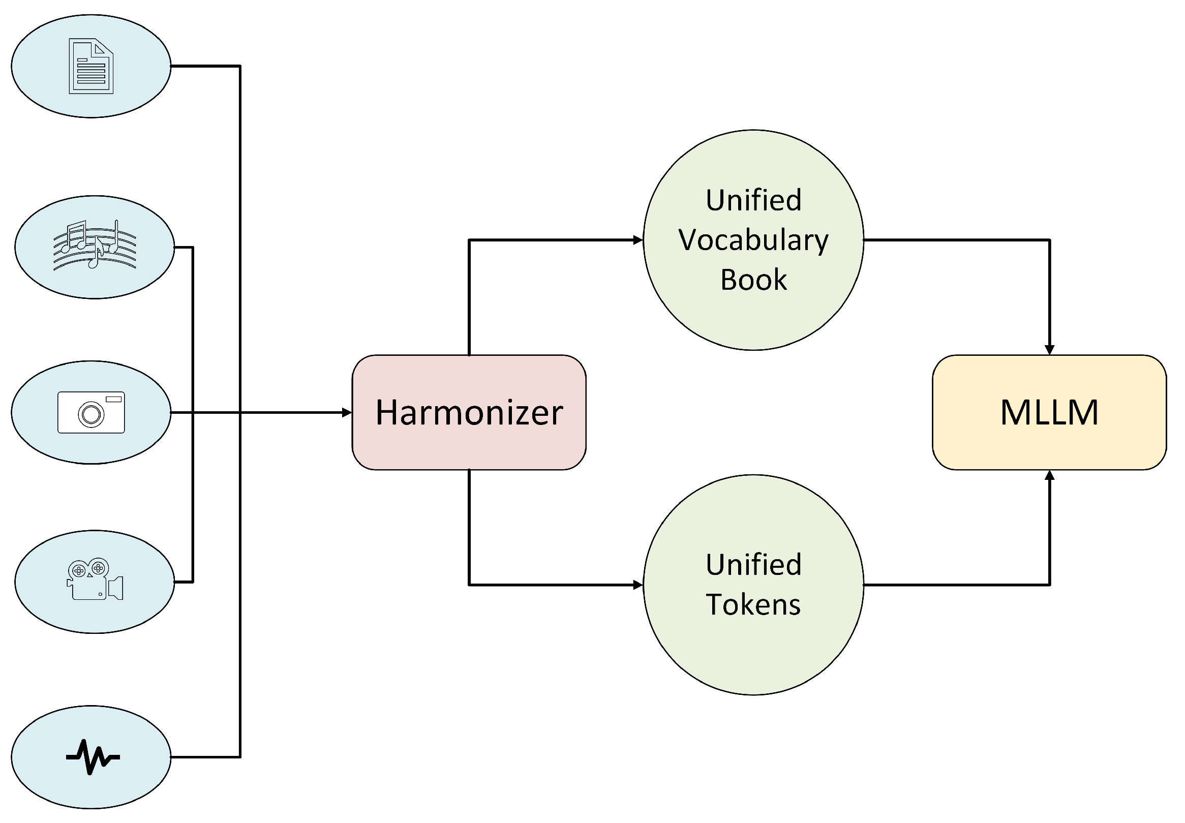
High-Level Architecture of the Harmonizer Framework. This schematic shows the end-to-end pipeline: (1) Input Preprocessing: raw text, audio, and video are converted into STFT spectrograms, analytic signals via the Hilbert transform, and contrast-enhanced via SCLAHE; (2) Feature Encoding: FluxHead applies streaming multi-head attention to extract temporal and spectral cues; (3) Tokenization: FusionQuantizer vector-quantizes these features into discrete tokens, building a learned signal vocabulary; (4) Streaming Inference: FluxFormer uses sliding-window transformers to generate tokens on-the-fly with minimal latency; (5) Optimization: a multi-objective loss (adversarial, L1/L2 time-domain, STFT/Hilbert/SCLAHE spectral, and perceptual) refines reconstruction quality. The final output is a unified token sequence that any multimodal LLM can consume without additional modality-specific encoders.
Mathematics 13 01819 g001
Figure 2. Overlaid left-channel waveforms for a 0.25 s excerpt of low-tempo, low-dynamic vocal music (3.50–3.75 s). The solid blue trace shows the ground-truth signal, while the dashed red trace shows the Harmonizer reconstruction. The near-perfect alignment of peaks, troughs, and transient edges demonstrates high temporal fidelity and minimal phase distortion introduced by the quantization and decoding pipeline.
Mathematics 13 01819 g002
Figure 3. Overlaid right-channel waveforms for a 0.25 s excerpt of low-tempo, low-dynamic vocal music (3.50–3.75 s). The solid green trace shows the ground-truth signal, while the dashed purple trace shows the Harmonizer reconstruction. The near-complete overlap of the two traces indicates excellent amplitude and phase fidelity across stereo channels.
Mathematics 13 01819 g003
Figure 4. Pixelwise spectrogram error percentage for the left channel of a low-tempo, low-dynamic music excerpt (clamped at the 95th percentile). The color scale indicates reconstruction error in each time-frequency bin, with most bins below 18%, demonstrating that Harmonizer maintains spectral integrity with only minor deviations.
Mathematics 13 01819 g004
Figure 5. Pixelwise spectrogram error percentage for the right channel of low-tempo, low-dynamic music (values clamped at the 95th percentile). The majority of time-frequency bins exhibit reconstruction errors below 18%, demonstrating consistent spectral fidelity across both stereo channels.
Mathematics 13 01819 g005
Figure 6. Absolute pixelwise spectrogram error for low-dynamic music’s left channel, displayed on a logarithmic color scale to highlight subtle discrepancies across time and frequency.
Mathematics 13 01819 g006
Figure 7. Absolute pixelwise spectrogram error for low-dynamic music (right channel), shown on a logarithmic color scale to amplify subtle discrepancies across time and frequency bins.
Mathematics 13 01819 g007
Figure 8. Comparison of Mel-Frequency Cepstral Coefficients for ground truth and regenerated low-tempo, low-dynamic music in left and right channels. Near-identical envelope shapes and temporal patterns indicate accurate preservation of timbral characteristics across both channels.
Mathematics 13 01819 g008
Figure 9. Difference between ground-truth and regenerated MFCCs for low-tempo, low-dynamic music. Light regions indicate near-zero deviation in cepstral coefficients across time and frequency, while the subtle band of warmer hues in lower frequencies highlights a minor residual mismatch that remains perceptually negligible.
Mathematics 13 01819 g009
Figure 10. MFCC error percentage (GT vs. Gen) for low-tempo, low-dynamic music with logarithmic color-bar. The predominantly blue color indicates negligible errors after clamping the 95th percentile to avoid outliers, with the maximum error reaching only about 5%.
Mathematics 13 01819 g010
Figure 11. Ground truth (GT) vs. generated (Gen) spectrograms for low-tempo, low-dynamic music. The top row represents left-channel spectrograms, while the bottom row represents right-channel spectrograms. Harmonizer preserves both broad spectral contours and finer harmonic details in low-amplitude passages. Quantitatively, over the full 288 s excerpt: left channel: PMSE = 1.4323, SSIM = 0.9887, PSNR = 47.96 dB; right channel: PMSE = 1.2548, SSIM = 0.9881, PSNR = 47.67 dB.
Mathematics 13 01819 g011
Figure 12. Overlaid waveforms—left channel (section 15: 3.50–3.75 s) for high-tempo, high-dynamic music. The red regenerated waveform tracks the blue ground truth waveform closely, indicating minimal temporal or amplitude distortion.
Mathematics 13 01819 g012
Figure 13. Overlaid waveforms—right channel (section 15: 3.50–3.75 s) for high-tempo, high-dynamic music. The purple regenerated waveform remains nearly indistinguishable from the green ground truth, reflecting robust transient alignment.
Mathematics 13 01819 g013
Figure 14. Ground truth (GT) vs. venerated (Gen) spectrograms for high-tempo, high-dynamic music. Harmonizer captures the broad dynamic range and maintains transient accuracy, matching key spectral features from 0 Hz to 16 kHz. Quantitatively, over the full 231 s excerpt: left channel: PMSE = 5.2295, SSIM = 0.9889, PSNR = 45.98 dB; right channel: PMSE = 5.4055, SSIM = 0.9892, PSNR = 46.09 dB; mean clamped spectrogram error = 15.2% (≈3.9%).
Mathematics 13 01819 g014
Figure 15. Pixelwise Spectrogram error percentage (clamped at 95th percentile)—left channel for high-tempo, high-dynamic music. The primary error range near 10–15% underscores Harmonizer’s capacity for accurate spectral reconstruction in rapidly changing signals. Mean clamped error = 15.2% ( σ ≈ 3.9%).
Mathematics 13 01819 g015
Figure 16. Pixelwise spectrogram error percentage (clamped at 95th percentile)—right channel for high-tempo, high-dynamic music. Similar to the left channel, most bins remain in a modest error range, corroborating stereo consistency. Quantitatively, the mean clamped error is 15.2% ( σ ≈ 3.9%).
Mathematics 13 01819 g016
Figure 17. Absolute pixelwise spectrogram error for high-dynamic music’s left channel, shown on a logarithmic color scale to emphasize subtle reconstruction deviations across frequency and time.
Mathematics 13 01819 g017
Figure 18. Absolute pixelwise spectrogram error for high-dynamic music’s right channel, depicted on a logarithmic color scale to highlight subtle reconstruction deviations across time and frequency.
Mathematics 13 01819 g018
Figure 19. Ground truth (GT) vs. generated (Gen) MFCCs for high-tempo, high-dynamic music. Harmonizer successfully captures complex spectral envelopes and abrupt changes, ensuring high perceptual fidelity. MFCC similarity = 0.9928.
Mathematics 13 01819 g019
Figure 20. MFCC difference (GT − Gen) for high-tempo, high-dynamic music. The near-zero difference across most frames confirms robust cepstral alignment, even in demanding signal contexts.
Mathematics 13 01819 g020
Figure 21. MFCC error percentage (GT vs. Gen) for high-tempo, high-dynamic music with logarithmic color-bar. The predominantly blue regions reflect near-zero error, with a maximum deviation of about 5%.
Mathematics 13 01819 g021
Figure 22. Comparison of original (blue) and reconstructed (red dashed) ASCII-encoded-Sinusoidal signals for text inputs of increasing length. Panels (ac) correspond, respectively, to single-word, two-token, and longer-sentence reconstructions.
Mathematics 13 01819 g022
Figure 23. Select frame comparisons and video link. (a) First frame—note crisp shapes and clear text with only minor block artifacts. (b) Last frame—demonstrates consistent reconstruction quality across the clip. (c) QR code linking to the full demonstration of all 16 frames, highlighting temporal coherence and overall video performance. The link to this video can be found in [134]. These preliminary results confirm that Harmonizer can process video inputs end-to-end; future work will focus on artifact reduction and temporal smoothing.
Mathematics 13 01819 g023
Figure 24. Overall token distribution. Token–ID bins (34 equal–width intervals spanning 0–1023) on the horizontal axis versus cumulative emission count across all 16 codebooks on the vertical axis. The pronounced peak at the highest bin (IDs 992–1023; 9000 counts) and the long tail toward low IDs are evident.
Mathematics 13 01819 g024
Figure 25. Codebooks 0–3. Codebook 0 exhibits a distinct peak around ID ≈ 500, deviating from the patterns observed in the others. Codebooks 1 through 3 all terminate with a pronounced spike at ID 1023. Notably, Codebook 1 displays two intermediate peaks prior to the terminal spike, Codebook 2 demonstrates a generally increasing trend with minor fluctuations, and Codebook 3 maintains a near-plateaued distribution before the final surge at ID 1023.
Mathematics 13 01819 g025
Figure 26. Codebooks 4–7. Codebook 4 exhibits an almost linear rise across IDs; Codebook 5 shows a moderate ramp before the final spike; Codebook 6 and 7 remain almost flat with some fluctuations until a steep jump near the end.
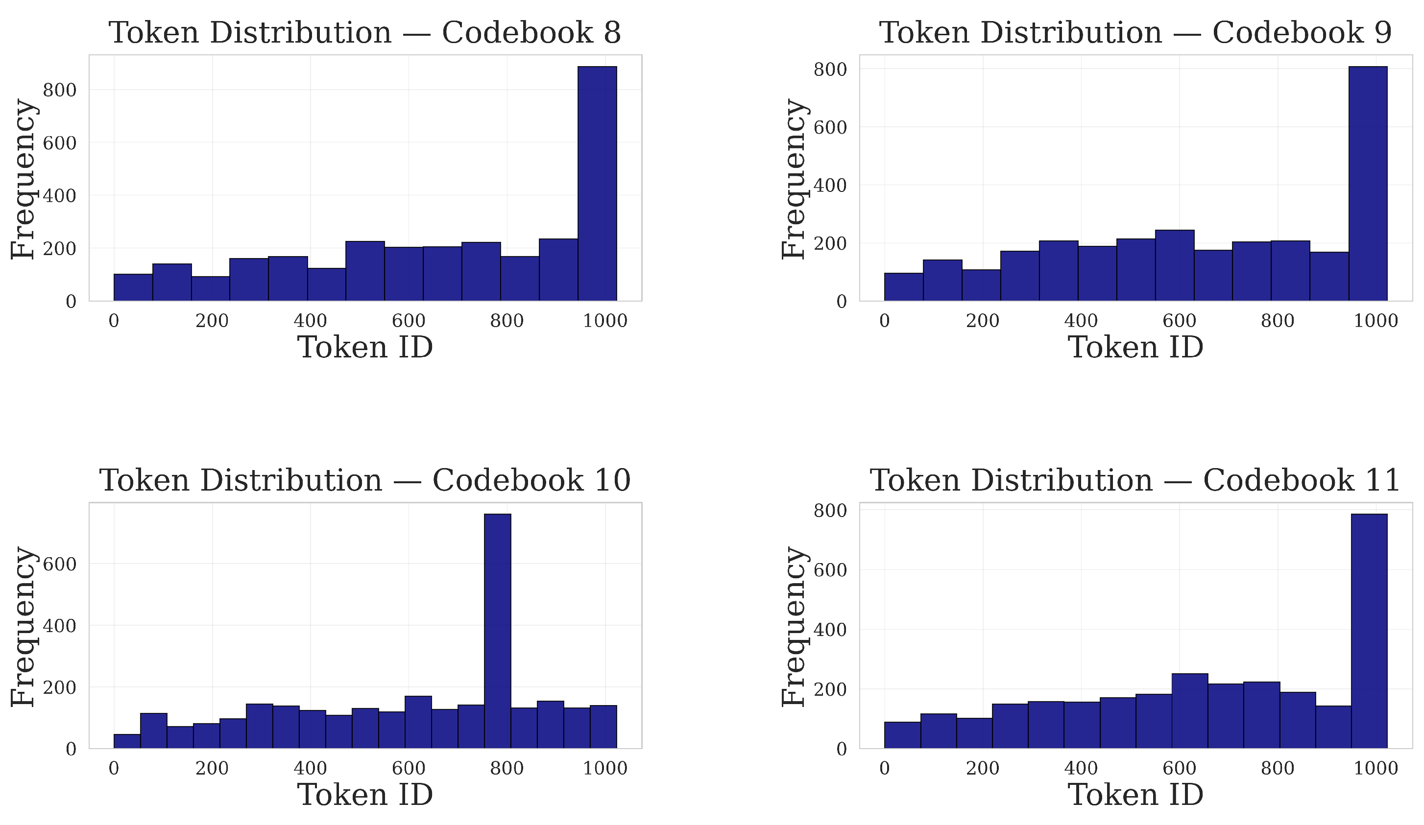
Mathematics 13 01819 g026
Figure 27. Codebooks 8–11. Codebook 8 shows a smooth, gentle rise; Codebook 9 is flat until a sharp final ascent; Codebook 10 features a different peak at ID ≈ 800; Codebook 11 presents a gradual midrange build then a pronounced spike.
Mathematics 13 01819 g027
Figure 28. Codebooks 12–15. Codebooks 12 and 15 feature gradual ramps with moderate slope before the significant terminal jump bar; Codebooks 13 and 14 exhibit small secondary peaks before the dominant terminal bar.
Mathematics 13 01819 g028aMathematics 13 01819 g028b
Figure 29. Application of Harmonizer as a Universal Multimodal Tokenizer in Large Language Models. The pipeline converts raw inputs—(a) text (ASCII → sine-encoded vectors), (b) audio (STFT → Hilbert → SCLAHE feature maps), and (c) video (spatiotemporal patches)—into a shared feature space. The FusionQuantizer then maps these continuous features to discrete token IDs via a learned codebook. During Streaming Inference, FluxFormer generates token sequences on the fly, which are interleaved or concatenated with standard text tokens and fed into cross-modal attention layers of the LLM. This unified token stream enables a single model to perform context-aware reasoning over text, audio, and video without separate modality-specific encoders.
Mathematics 13 01819 g029
Table 1. Normalized weights assigned to each component of the multi-objective loss function, ensuring their sum equals 1.0.
Loss TermWeight
α (Adversarial)0.10
β 1 ( L 1 )0.40
β 2 ( L 2 )0.20
γ (Perceptual)0.10
δ 0 (STFT)0.05
δ 1 (Hilbert)0.05
δ 2 (SCLAHE)0.10
Total1.00
Table 2. Detailed hyperparameter settings and hardware configurations used for training and evaluating the Harmonizer framework.
AspectSetting
Model size≈65 million parameters
OptimizerAdamW, lr = 1 × 10 5
Audio framing96 kHz stereo, 1 s segments, 0.5% overlap
Feature backbone128-dim features, 32 base channels
Quantization16 codebooks, 1024 entries each
Sequence model512-dim embeddings, 10 layers, 16 heads
Mixed precisionFP16/BF16 on A100 GPUs (TF32 fallback on P100)
Table 3. Quantitative evaluation metrics for audio reconstruction, listing each abbreviation, its full name, the numerical range of values, and the criterion for optimal performance; the lower section presents pixel-wise image-based metrics computed on spectrograms.
Abbr.Expanded VersionRangeOptimal Value
MSEMean Squared Error [ 0 , ) min ( MSE ) 0
CCCorrelation Coefficient [ 1 , 1 ] max ( CC ) 1
CSCosine Similarity [ 1 , 1 ] max ( CS ) 1
DTWDynamic Time Warping Distance [ 0 , ) min ( DTW ) 0
SCSpectral Convergence [ 0 , ) min ( SC ) 0
SNRSignal-to-Noise RatioTypically [ 0 , ) (dB) max ( SNR )
LSDLog-Spectral Distance [ 0 , ) min ( LSD ) 0
MFCCMFCC Similarity [ 0 , 1 ] max ( MFCC ) 1
PMSEPixelwise MSE [ 0 , ) min ( PMSE ) 0
SSIMStructural Similarity Index Measure [ 0 , 1 ] max ( SSIM ) 1
PSNRPeak Signal-to-Noise Ratio [ 0 , ) (dB) max ( PSNR )
Table 4. Quantitative performance metrics for low-tempo, low-dynamic vocal music signals (≈288 s), covering time-domain error (MSE, CC, CS), temporal alignment (DTW), spectral fidelity (SC, LSD, MFCC), signal-to-noise ratios (SNRs), and pixelwise spectrogram measures (PMSE, SSIM, PSNR) for both stereo channels.
MetricValue
MSE 3.6645 × 10 3
Correlation Coefficient (CC) 0.9282
Cosine Similarity (Left/Right) 0.9988 / 0.9993
DTW Distance (Left/Right) 12.12 / 11.91
Spectral Convergence (Left/Right) 0.3021 / 0.2906
SNR (Reconstructed) 8.50 dB
LSD (Left/Right) 6.350 / 6.401
MFCC Similarity 0.9965
SNR (Ground Truth/Generated) 24.14 dB/ 22.99 dB
Left Pixelwise MSE 1.4323
Left Pixelwise SSIM 0.9887
Left Pixelwise PSNR 47.96 dB
Right Pixelwise MSE 1.2548
Right Pixelwise SSIM 0.9881
Right Pixelwise PSNR 47.67 dB
Table 5. Quantitative performance metrics for high-tempo, high-dynamic vocal music signals (≈231 s), covering time-domain error (MSE, CC, CS), temporal alignment (DTW), spectral fidelity (SC, LSD, MFCC), signal-to-noise ratios (SNRs), and pixelwise spectrogram measures (PMSE, SSIM, PSNR) for both stereo channels.
MetricValue
MSE 1.0511 × 10 2
Correlation Coefficient (CC) 0.9468
Cosine Similarity (Left/Right) 0.9968 / 0.9967
DTW Distance (Left/Right) 8.0186 / 7.7819
Spectral Convergence (Left/Right) 0.3904 / 0.3897
SNR (Reconstructed) 8.67 dB
LSD (Left/Right) 6.8276 / 6.8498
MFCC Similarity 0.9928
SNR (Ground Truth/Generated) 28.89 dB/ 26.58 dB
Left Pixelwise MSE 5.2295
Left Pixelwise SSIM 0.9889
Left Pixelwise PSNR 45.98 dB
Right Pixelwise MSE 5.4055
Right Pixelwise SSIM 0.9892
Right Pixelwise PSNR 46.09 dB
Table 6. Comparison of speech reconstruction quality on the VCTK test set, showing Short-Time Objective Intelligibility (STOI) and Perceptual Evaluation of Speech Quality (PESQ), where higher values indicate better performance.
ModelSTOI (↑)PESQ (↑)
Encodec [125]0.812.00
DAC [132]0.812.10
WavTokenizer [128]0.791.90
StableCodec  [133]0.761.80
ALMTokenizer [131]0.812.00
SemantiCodec [130]0.811.76
Harmonizer (ours)0.902.30
Note: ↑ indicates that higher values are better. Bold font highlights the best performance.
Table 7. Music reconstruction performance on the MusicCaps dataset, reporting mean Mel-spectrogram loss and STFT reconstruction loss (↓).
ModelMel-Spectrogram Loss (↓)STFT Reconstruction Loss (↓)
Encodec [125]34.81.26
DAC [132]35.91.28
WavTokenizer [128]48.21.47
ALMTokenizer [131]34.41.32
SemantiCodec [130]47.91.58
Harmonizer (ours)16.91.34
Note: ↓ indicates that lower values are better. Bold font highlights the best performance.
Table 8. Comparison of key reconstruction metrics between low-tempo/low-dynamic and high-tempo/high-dynamic music signals.
MetricLow-Tempo
Low-Dynamic
High-Tempo
High-Dynamic
MSE 3.66 × 10 3 1.05 × 10 2
Correlation Coefficient (CC) 0.9282 0.9468
Cosine Similarity (L/R) 0.9988 / 0.9993 0.9968 / 0.9967
DTW Distance (L/R) 12.12 / 11.91 8.02 / 7.78
Spectral Convergence (L/R) 0.3021 / 0.2906 0.3904 / 0.3897
MFCC Similarity 0.9997 0.9928
Mean Pixelwise MSE (L/R) 1.43 / 1.25 5.23 / 5.41
Mean Pixelwise SSIM (L/R) 0.9887 / 0.9881 0.9889 / 0.9892
Mean Pixelwise PSNR (dB) (L/R) 47.96 / 47.67 45.98 / 46.09
Disclaimer/Publisher’s Note: The statements, opinions and data contained in all publications are solely those of the individual author(s) and contributor(s) and not of MDPI and/or the editor(s). MDPI and/or the editor(s) disclaim responsibility for any injury to people or property resulting from any ideas, methods, instructions or products referred to in the content.

