A Fast Proximal Alternating Method for Robust Matrix Factorization of Matrix Recovery with Outliers

Abstract

This paper concerns a class of robust factorization models of low-rank matrix recovery, which have been widely applied in various fields such as machine learning and imaging sciences. An ${\ell }_1$-loss robust factorized model incorporating the ${\ell }_{2,0}$-norm regularization term is proposed to address the presence of outliers. Since the resulting problem is nonconvex, nonsmooth, and discontinuous, an approximation problem that shares the same set of stationary points as the original formulation is constructed. Subsequently, a proximal alternating minimization method is proposed to solve the approximation problem. The global convergence of its iterate sequence is also established. Numerical experiments on matrix completion with outliers and image restoration tasks demonstrate that the proposed algorithm achieves low relative errors in shorter computational time, especially for large-scale datasets.

1. Introduction

The low-rank matrix recovery problem seeks to recover a true yet unknown low-rank matrix $M^{\ast }$ of rank $r^{\ast }$ from the minimal feasible observations. This problem encompasses various applications in numerous fields, including signal and image processing, quantum state tomography, control and system identification, statistics, machine learning, etc. (see [1,2,3,4,5]). This paper considers a robust factorized model for the low-rank matrix recovery problem, in which the observations contain outliers. The model is expressed as

$$b=\mathcal{A}(M^{\ast })+\omega ,$$

where $\mathcal{A}:{\mathbb{R}}^{n_1\times n_2}\to {\mathbb{R}}^m$ is a sampling operator, $b\in {\mathbb{R}}^m$ is the observation vector, and $\omega$ is a sparse noise vector with arbitrarily large nonzero entries, while the rest of the elements are zero. In scenarios where outliers exist, the traditional smooth least-squared loss function becomes too sensitive to outliers and is probably biased. In view of this, studies [6,7] have proposed a non-smooth ${\ell }_p$-loss with balance regularization model:

$$\begin{array}{c}\hfill \underset{U\in {\mathbb{R}}^{n_1\times \kappa },V\in {\mathbb{R}}^{n_2\times \kappa }}{min}\Psi (U,V):=\parallel \mathcal{A}(U{V}^{\top }){-b\parallel }_p+\gamma {\parallel U{U}^{\top }-V{V}^{\top }\parallel }_F,\end{array}$$

(1)

where $\gamma \ge 0$. When $\gamma >0$, for $p=1$ and $\kappa =r^{\ast }$, Li et al. [7] established exact matrix recovery based on the ${\ell }_1/{\ell }_2$-restricted isometry property of the sampling operator $\mathcal{A}$ and proved that the proposed subgradient method with geometrically diminishing step sizes converges linearly to the ground-truth matrix. For $p=1$ or 2 and $\kappa =r^{\ast }$, Charisopoulos et al. [6] proved that the subgradient method and prox-linear method converge at a fast dimension-independent rate under the same assumptions as in [7]. When $\gamma =0$, for $p=1$, Ma and Fattahi [8] showed that the subgradient method converges to the true matrix under the Sign-RIP condition [[8], Definition 7]. Additionally, Wang et al. [9] developed a robust and fast rank-one matrix completion algorithm by minimizing the Welsch cost function.

Although the subgradient method exhibits favorable convergence properties in solving the problem (1), it is limited by some strict assumptions. Practically, the rank of the ground-truth matrix is generally unknown, and consequently, the regularization term in (1) fails to induce low-rank structures. Inspired by [10], this paper utilizes the ${\ell }_{2,0}$-norm in the regularization term and studies the following ${\ell }_1$-loss factorized model of low-rank matrix recovery:

$$\begin{array}{c}\hfill \underset{U\in {\mathbb{R}}^{n_1\times \kappa },V\in {\mathbb{R}}^{n_2\times \kappa }}{min}\Phi (U,V):=\parallel \mathcal{A}(U{V}^{\top }){-b\parallel }_1+{\lambda (\parallel U\parallel }_{2,0}+{\parallel V\parallel }_{2,0}),\end{array}$$

(2)

where $\kappa$ is an upper estimator of $r^{\ast }$, and ${\parallel ·\parallel }_{2,0}$ denotes the ${\ell }_{2,0}$-norm of matrices, which measures the number of the nonzero column. The regularization term $\lambda (\parallel U{\parallel }_{2,0}+\parallel V{\parallel }_{2,0})$ is used to reduce rank through column sparsity. The ${\ell }_1$-loss function, on the other hand, is more robust against outliers and has been widely utilized for outlier detection studies [11,12,13]. Both terms of the objective function (2) are nonsmooth. On top of that, the function suffers from both nonconvexity and discontinuity due to the existence of the ${\ell }_{2,0}$-norm regularization term. The discontinuity causes the subgradient algorithm to fail when it is applied to problem (2). While the alternating direction method of multipliers is commonly applied to address problem (2), there is still no theoretical guarantee of its convergence in the context of such nonconvex and nonsmooth optimization problems. For methods with convergence guarantees, the majority of them impose, within their objective functions, either the assumption of smoothness for at least one term or the continuity assumption. To the best of our knowledge, no state-of-the-art algorithm is capable of handling this type of nonconvex and discontinuous problem.

The major contributions of this work are threefold. Firstly, to handle the nonconvex and discontinuous problem (2), a novel potential function is constructed:

$$\begin{array}{c}\hfill \underset{U\in {\mathbb{R}}^{n_1\times \kappa },V\in {\mathbb{R}}^{n_2\times \kappa },z\in {\mathbb{R}}^m}{min}\Theta (U,V,z):={\displaystyle \frac{\alpha }{2}}\parallel \mathcal{A}(U{V}^{\top }){-b-z\parallel }^2+{\parallel z\parallel }_1+{\lambda (\parallel U\parallel }_{2,0}+{\parallel V\parallel }_{2,0}),\end{array}$$

(3)

where $\alpha >0$ is a given constant. It has been proven that, under mild assumptions, the sets of stationary points of (2) and (3) are equivalent. Moreover, it has been demonstrated that any global optimal solution to problem (3) is an approximate optimal solution to problem (2). This equivalence enables us to find solutions to problem (2) by solving problem (3), and the latter is more computationally efficient. Secondly, a proximal alternating linearized minimization (PALM) method is proposed to solve (3). The global convergence of PALM method is also established by exploiting the Kurdyka–Łojasiewicz (KL) property of the objective function. Finally, numerical experiments conducted on both synthetic and real-world datasets have validated that the PALM method for problem (3) outperforms SubGM [6,7] for problem (1) with $p=1$.

The remainder of this paper is organized as follows. Section 2 introduces preliminaries and foundational concepts. In Section 3, the relationship between problems (2) and (3) is established. Section 4 presents the PALM method to solve the problem (3), with its global convergence established. In Section 5, the numerical performance of the PALM method is evaluated, and its performance is compared with that of SubGM to solve the problem (1) through experiments on various datasets. Section 6 concludes the paper.

2. Preliminaries

This section introduces the notation employed and then presents the definitions of stationary points and the KL property.

2.1. Notations

Throughout this paper, ${\mathbb{R}}^{n_1\times n_2}$ represents the vector space of all $n_1\times n_2$ real matrices, equipped with the trace inner product $\langle X,Y\rangle =\mathrm{trace}(X^{\top }Y)$ for $X,Y\in {\mathbb{R}}^{n_1\times n_2}$ and its induced Frobenius norm. For a matrix $X\in {\mathbb{R}}^{n_1\times n_2}$, $Z_j$ denotes the jth column of Z, $J_Z$ represents its index set of nonzero columns, and ${\parallel X\parallel }_F$ and ${\parallel X\parallel }_{2,0}$ denote the Frobenius norm and the column ${\ell }_{2,0}$-norm of X, which means the number of nonzero columns. For a matrix $X\in {\mathbb{R}}^{n_1\times n_2}$, let $\sigma (X):={({\sigma }_1(X),\dots ,{\sigma }_n(X))}^{\top }$ with ${\sigma }_1(X)\ge \cdots \ge {\sigma }_n(X)$, where ${\sigma }_i(X)$ denotes the singular value of X, ${\Sigma }_{\kappa }(X):=\mathrm{Diag}({\sigma }_1(x),\dots ,{\sigma }_{\kappa }(X))$. For a vector $x\in {\mathbb{R}}^n$, ${\parallel x\parallel }_1$ denotes the ${\ell }_1$-norm and $\parallel x\parallel$ denotes the ${\ell }_2$-norm. Let ${\nabla }_{U}F(U,V)$ and ${\nabla }_{V}F(U,V)$ denote the partial gradient of F at $(U,V)$ w.r.t. variable U and V, respectively. For any $x\in {\mathbb{R}}^m$, $\mathrm{sign}(x)=[\mathrm{sign}(x_1),\cdots ,\mathrm{sign}(x_m)]$ with

$$\mathrm{sign}(t):=\left\{\begin{array}{cc}t/|t|,& t\ne 0;\hfill \\ 0,& t=0.\hfill \end{array}\right.\mathrm{for}\mathrm{any}t\in \mathbb{R}.$$

For convenience, define $G(U,V,z):={\displaystyle \frac{\alpha }{2}}{\parallel \mathcal{A}(U{V}^{\top })-b-z\parallel }^2$,

$$F(U,V):=\parallel \mathcal{A}(U{V}^{\top }){-b\parallel }_1\mathrm{and}g(U):={\parallel U\parallel }_{2,0}.$$

2.2. Stationary Points and $ϵ$-Global Optimal Solutions

From [14], the generalized subdifferentials of an extended real-valued function h: ${\mathbb{R}}^{n\times m}\to \overline{\mathbb{R}}:=(-\infty ,\infty ]$ at a point where h attains a finite value are recalled.

Definition 1.

Given a function $h:{\mathbb{R}}^{n\times m}\to \overline{\mathbb{R}}$ with a point x such that $h(x)$ is finite. The regular subdifferential of h at x is defined as follows:

$$\widehat{\partial }h(x):=\left\{v\in {\mathbb{R}}^{n\times m}|\underset{x\ne x^{\prime }\to x}{lim\; inf}{\displaystyle \frac{h(x^{\prime })-h(x)-\langle v,x^{\prime }-x\rangle }{\parallel x^{\prime }{-x\parallel }_F}}\ge 0\right\},$$

and the basic (or, say, limiting or Morduhovich) subdifferential of h at x is defined as

$$\partial h(x):=\left\{v\in {\mathbb{R}}^{n\times m}|\exists x^k\to x\mathrm{with}h(x^k)\to h(x)\mathrm{and}{v}^k\to v\mathrm{with}{v}^k\in \widehat{\partial }h(x^k)\right\}.$$

Consider a proper lower semicontinuous (lsc) function $h:{\mathbb{R}}^{n\times m}\to \overline{\mathbb{R}}$, the stationary point and $ϵ$-global optimal solution to problem $\underset{x\in {\mathbb{R}}^{n\times m}}{min}h(x)$ are defined as follows.

Definition 2.

For a point $x\in {\mathbb{R}}^{n\times m}$ such that $0\in \partial h(x)$, it is called a stationary point of $\underset{x\in {\mathbb{R}}^{n\times m}}{min}h(x)$.

Definition 3.

For a point $x^{\ast }\in {\mathbb{R}}^{n\times m}$ such that

$$h(x^{\ast })-ϵ\le h(x)\forall x\in {\mathbb{R}}^{n\times m},$$

it is called an ϵ-global optimal solution of $\underset{x\in {\mathbb{R}}^{n\times m}}{min}h(x)$.

2.3. Kurdyka–Łojasiewicz Property

From [15], the KL property of an extended real-valued function is stated as follows.

Definition 4.

Given $h:\mathbb{X}\to \overline{\mathbb{R}}$ a proper lsc function. It is said to have the Kurdyka–Łojasiewicz (KL) property at $\overline{x}\in \mathrm{dom}\partial h$ if there exists $\eta \in (0,\infty ]$; a continuous concave function $\phi :[0,\eta )\to {\mathbb{R}}_{+}$ satisfies

(i) 

$\phi (0)=0$ and φ is continuously differentiable on $(0,\eta )$, and

(ii) 

$\forall s\in (0,\eta )$, ${\phi }^{\prime }(s)>0$;

and a neighborhood $\mathcal{U}$ of $\overline{x}$ such that $\forall x\in \mathcal{U}\cap \left[h(\overline{x})<h(x)<h(\overline{x})+\eta \right],$

$${\phi }^{\prime }(h(x)-h(\overline{x}))\mathrm{dist}(0,\partial h(x))\ge 1.$$

If the function h satisfies the KL property at any points of $\mathrm{dom}\partial h$, then h is called a KL function.

Remark 1.

According to Lemma 2.1 of [15], a proper lsc function has the KL property at any noncritical point. Thus, to prove that a proper lsc function $h:\mathbb{X}\to \overline{\mathbb{R}}$ is a KL function, it suffices to check whether h has the KL property at any critical point.

3. Relationship Between Problems (2) and (3)

This section demonstrates the relationship between the stationary points and global optimal solutions of (2) and (3). On top of that, the stationary point sets of (2) and (3) are characterized. The subdifferential of $\Phi$ at an arbitrary point $(U,V)\in {\mathbb{R}}^{n_1\times \kappa }\times {\mathbb{R}}^{n_2\times \kappa }$ is given in the following lemma.

Lemma 1.

Fix any $\lambda >0$. Consider any $(U,V)\in {\mathbb{R}}^{n_1\times \kappa }\times {\mathbb{R}}^{n_2\times \kappa }$. Then, it holds that

$$\begin{array}{c}\hfill \widehat{\partial }\Phi (U,V)=\partial \Phi (U,V)=\left\{\left(\begin{array}{c}{\mathcal{A}}^{\ast }(\xi )V+\lambda \partial g(U)\\ {\left[{\mathcal{A}}^{\ast }(\xi )\right]}^{\top }U+\lambda \partial g(V)\end{array}\right)|\xi \in \partial {\parallel ·\parallel }_1\left(\mathcal{A}(U{V}^{\top })-b\right)\right\},\end{array}$$

where for any $X\in {\mathbb{R}}^{n\times m}$

$$\widehat{\partial }g(X)=\partial g(X)=S_1\times \cdots \times S_m\mathrm{with}{S}_j=\left\{\begin{array}{cc}{\{0\}}^n& \mathrm{if}j\in J_X;\hfill \\ {\mathbb{R}}^n& \mathrm{if}j\notin J_X.\hfill \end{array}\right.$$

Proof. 

Recall that $\Phi (U,V)=F(U,V)+\lambda (g(U)+g(V))$. From [[14], Corollary 10.9 and Exercise 10.10], it immediately follows that

$$\begin{array}{ll}\widehat{\partial }F(U,V)+\lambda \widehat{\partial }g(U)\times \lambda \widehat{\partial }g(V)& \subset \widehat{\partial }\Phi (U,V)\subset \partial \Phi (U,V)\\ & \subset \partial F(U,V)+\lambda \partial g(U)\times \lambda \partial g(V).\end{array}$$

Next, $\partial F(U,V)$ and $\widehat{\partial }F(U,V)$ are calculated. According to the chain rule [[14], Corollary 8.11 and Theorem 10.6], we obtain

$$\begin{array}{c}\hfill \partial F(U,V)=\widehat{\partial }F(U,V)=\left\{\left(\begin{array}{c}{\mathcal{A}}^{\ast }(\xi )V\\ {\left[{\mathcal{A}}^{\ast }(\xi )\right]}^{\top }U\end{array}\right)|\xi \in \partial {\parallel ·\parallel }_1\left(\mathcal{A}(U{V}^{\top })-b\right)\right\}.\end{array}$$

For any $U\in {\mathbb{R}}^{n_1\times \kappa }$, by invoking [[14], Proposition 10.5], it immediately follows that

$$\widehat{\partial }g(U)=\partial g(U)=S_1\times \cdots \times S_{\kappa }\mathrm{with}{S}_j=\left\{\begin{array}{cc}{\{0\}}^{n_1}& \mathrm{if}j\in J_U;\hfill \\ {\mathbb{R}}^{n_1}& \mathrm{if}j\notin J_U.\hfill \end{array}\right.$$

(4)

This, along with the inclusion above, implies that the desired result holds. □

The subdifferential of $\Theta$ is characterized by the following lemma.

Lemma 2.

Fix any $\lambda >0$. Consider any $(U,V,z)\in {\mathbb{R}}^{n_1\times \kappa }\times {\mathbb{R}}^{n_2\times \kappa }\times {\mathbb{R}}^m$. Then, it holds that

$$\begin{array}{c}\hfill \widehat{\partial }\Theta (U,V,z)=\partial \Theta (U,V)=\left(\begin{array}{c}\alpha {\mathcal{A}}^{\ast }(\mathcal{A}(U{V}^{\top })-b-z)V+\lambda \partial g(U)\\ \alpha {\left[{\mathcal{A}}^{\ast }(\mathcal{A}(U{V}^{\top })-b-z)\right]}^{\top }U+\lambda \partial g(V)\\ \alpha (z-\mathcal{A}(U{V}^{\top })+b)+\partial {\parallel z\parallel }_1\end{array}\right),\end{array}$$

where $\partial g$ is defined in Lemma 1.

Proof. 

Recall that $\Theta (U,V,z)=G(U,V,z)+{\parallel z\parallel }_1+\lambda (g(U)+g(V))$. Then, from [[14], Exercise 8.8(c) and Proposition 10.5], it immediately follows that

$$\begin{array}{cc}\hfill \nabla G(U,V,z)+\lambda \widehat{\partial }g(U)\times \lambda \widehat{\partial }g(V)\times \partial {\parallel z\parallel }_1& \subset \widehat{\partial }\Theta (U,V,z)\subset \partial \Theta (U,V,z)\hfill \\ \hfill & \subset \nabla G(U,V,z)+\lambda \partial g(U)\times \lambda \partial g(V)\times {\partial \parallel z\parallel }_1.\hfill \end{array}$$

By the smoothness and the expression of $G(U,V,z)$, one has

$$\begin{array}{c}\hfill \nabla G(U,V,z)=\left(\begin{array}{c}\alpha {\mathcal{A}}^{\ast }(\mathcal{A}(U{V}^{\top })-b-z)V\\ \alpha {\left[{\mathcal{A}}^{\ast }(\mathcal{A}(U{V}^{\top })-b-z)\right]}^{\top }U\\ \alpha (z-\mathcal{A}(U{V}^{\top })+b)\end{array}\right).\end{array}$$

Along with the above inclusion and (4), the desired results are obtained. □

The following proposition states the equivalence between the stationary points of problems (2) and (3) under some mild conditions.

Proposition 1.

If $(U,V,z)\in {\mathbb{R}}^{n_1\times \kappa }\times {\mathbb{R}}^{n_2\times \kappa }\times {\mathbb{R}}^m$ is an arbitrary stationary point of (3) satisfying the nonzero elements of $|\mathcal{A}(U{V}^{\top })-b|$ not smaller than ${\displaystyle \frac{1}{\alpha }}$, then $(U,V)$ is a stationary point of (2). Conversely, if $(U,V)\in {\mathbb{R}}^{n_1\times \kappa }\times {\mathbb{R}}^{n_2\times \kappa }$ is an arbitrary stationary point of (2) satisfying all elements of $|\mathcal{A}(U{V}^{\top })-b|$ not smaller than ${\displaystyle \frac{1}{\alpha }}$, then there exists $z\in \mathcal{A}(U{V}^{\top })-b-\mathrm{sign}\left(\mathcal{A}(U{V}^{\top })-b\right)$ such that $(U,V,z)$ is a stationary point of (3).

Proof. 

Pick any stationary point $(U,V,z)$ of (3). From Lemma 2, it holds that

$$\{\begin{array}{ll}0\in \alpha {\mathcal{A}}^{\ast }(\mathcal{A}\left({UV}^{\top }\right)-b-z)V+\lambda \partial g\left(U\right);& \mathrm{(5a)}\\ 0\in \alpha {[{\mathcal{A}}^{\ast }(\mathcal{A}\left({UV}^{\top }\right)-b-z)]}^{\top }U+\lambda \partial g\left(V\right);& \mathrm{(5b)}\\ 0\in -\alpha (\mathcal{A}\left({UV}^{\top }\right)-b-z)+\partial {\Vert z\Vert }_1.& \mathrm{(5c)}\end{array}$$

Write $y:=\mathcal{A}(U{V}^{\top })-b$. From (5c), it can be concluded that $z=\mathrm{sign}(y)\circ max\left(0,|y|-{\displaystyle \frac{1}{\alpha }}\right)$. Then,

$$y-z=\mathrm{sign}(y)\circ min(|y|,{\displaystyle \frac{1}{\alpha }}),$$

(6)

Along with $|y_i| \ge {\displaystyle \frac{1}{\alpha }}$ or $y_i=0$ for all $i=1,\dots ,m$, one has $y-z={\displaystyle \frac{1}{\alpha }}\mathrm{sign}(y)$. Thus, substituting $y-z={\displaystyle \frac{1}{\alpha }}\mathrm{sign}(y)$ into (5a) and (5b), one obtains

$$\left\{\begin{array}{c}0\in {\mathcal{A}}^{\ast }\left(\mathrm{sign}\left(\mathcal{A}(U{V}^{\top })-b\right)\right)V+\lambda \partial g(U);\hfill \\ 0\in {\left[{\mathcal{A}}^{\ast }\left(\mathrm{sign}\left(\mathcal{A}(U{V}^{\top })-b\right)\right)\right]}^{\top }U+\lambda \partial g(V).\hfill \end{array}\right.$$

This together with the definition of $\mathrm{sign}(·)$ implies that $(U,V)$ is a stationary point of (2).

Conversely, any $(U,V)$ is a stationary point of (2). According to Lemma 1, there exists ${\xi \in \partial \parallel ·\parallel }_1\left(\mathcal{A}(U{V}^{\top })-b\right)$ such that

$$\left\{\begin{array}{c}0\in {\mathcal{A}}^{\ast }(\xi )V+\lambda \partial g(U)\hfill \\ 0\in {\left[{\mathcal{A}}^{\ast }(\xi )\right]}^{\top }U+\lambda \partial g(V)\hfill \end{array}\right.$$

Write $y:=\mathcal{A}(U{V}^{\top })-b$ and $z:=y-{\displaystyle \frac{1}{\alpha }}\xi$. Then, $(U,V,z)$ satisfies (5a) and (5b). By noting that $|{\xi }_i| \le 1$ for all $i=1,\dots ,m$, and $|y_i| \ge {\displaystyle \frac{1}{\alpha }}$ for all $i=1,\dots ,m$, one has $\alpha (y-z)={\xi \in \partial \parallel ·\parallel }_1(y-{\displaystyle \frac{1}{\alpha }}\xi )=\partial {\parallel z\parallel }_1$ which means that (5c) holds. This implies that $(U,V,z)$ is a stationary point of (3). The proof is completed. □

Remark 2.

The converse of the above property generally does not hold, as the obtained vector y is expected to be sparse. This indicates that the set of stationary points for problem (3) is typically smaller than that of problem (2). Through the relationship between the global optimal solutions of (2) and (3) in next proposition, the stationary points of (3) exclude certain undesirable points contained in the stationary point set of (2).

Proposition 2.

If $(U^{\ast },V^{\ast },z^{\ast })$ is a global optimal solution of (3), then $(U^{\ast },V^{\ast })$ is a ${\displaystyle \frac{m}{2\alpha }}$-global optimal solution of (2).

Proof. 

If $(U^{\ast },V^{\ast },z^{\ast })$ is a global optimal solution of (3), then $(U^{\ast },V^{\ast },z^{\ast })$ is a stationary point of (3). Write $y^{\ast }:=\mathcal{A}(U^{\ast }{(V^{\ast })}^{\top })-b$. From (6), it holds that

$$y^{\ast }-z^{\ast }=\mathrm{sign}(y^{\ast })\circ min(|y^{\ast }|,{\displaystyle \frac{1}{\alpha }}).$$

Let $I:=\{i\in \left[m\right]||y_i^{\ast }|<{\displaystyle \frac{1}{\alpha }}\}$ and $\overline{I}:=\{i\in \left[m\right]||y_i^{\ast }|\ge {\displaystyle \frac{1}{\alpha }}\}$. Then, one has

$$\begin{array}{cc}\hfill G(U^{\ast },V^{\ast },z^{\ast })=& {\displaystyle \frac{\alpha }{2}}\parallel y^{\ast }-z^{\ast }{\parallel }^2+{\parallel z^{\ast }\parallel }_1\hfill \\ \hfill =& {\displaystyle \frac{\alpha }{2}}\parallel \mathrm{sign}(y^{\ast })\circ min(|y^{\ast }|,{\displaystyle \frac{1}{\alpha }}{)\parallel }^2+\parallel \mathrm{sign}(y^{\ast })\circ max\left(0,|y^{\ast }|-{\displaystyle \frac{1}{\alpha }}\right){\parallel }_1\hfill \\ \hfill =& {\displaystyle \frac{\alpha }{2}}\sum _{i\in I}|y_i^{\ast }{|}^2+\sum _{i\in \overline{I}}(|y_i^{\ast }|-{\displaystyle \frac{1}{2\alpha }})\hfill \\ \hfill =& \parallel y^{\ast }{\parallel }_1-{\displaystyle \frac{m}{2\alpha }}+\sum _{i\in I}({\displaystyle \frac{\alpha }{2}}|y_i^{\ast }{|}^2-|y_i^{\ast }|+{\displaystyle \frac{1}{2\alpha }})\ge \parallel y^{\ast }{\parallel }_1-{\displaystyle \frac{m}{2\alpha }},\hfill \end{array}$$

where the inequality is due to $|y_i^{\ast }|<{\displaystyle \frac{1}{\alpha }}$ for $i\in I$. Since $(U^{\ast },V^{\ast },z^{\ast })$ is a global optimal solution of (3), for any $(U,V,z)$ with $z=\mathcal{A}(U{V}^{\top })-b$

$$\begin{array}{c}\hfill \Phi (U^{\ast },V^{\ast })-{\displaystyle \frac{m}{2\alpha }}\le \Theta (U^{\ast },V^{\ast },z^{\ast })\le \Theta (U,V,z)=\Phi (U,V).\end{array}$$

This means that $(U^{\ast },V^{\ast },z^{\ast })$ is a ${\displaystyle \frac{m}{2\alpha }}$-global optimal solution of (2).    □

Remark 3.

Proposition 2 demonstrates that global optimal solution $(U^{\ast },V^{\ast },z^{\ast })$ of problem (3) is an approximate optimal solution to problem (2), and as the parameter α increases, the value $\Phi (U^{\ast },V^{\ast })$ progressively approaches the optimal value of problem (2).

4. A PALM Method for Solving Problem (3)

Recall that $G(U,V,z)={\displaystyle \frac{\alpha }{2}}{\parallel \mathcal{A}(U{V}^{\top })-b-z\parallel }^2$ is a smooth function. The gradients ${\nabla }_{U}G(·,V,z)$ and ${\nabla }_{V}G(U,·,z)$ are Lipschitz continuous with moduli defined as ${\tau }_V$ and ${\tau }_U$, respectively. Fix any $(U^{\prime },V^{\prime },z^{\prime })\in {\mathbb{R}}^{n_1\times \kappa }\times {\mathbb{R}}^{n_2\times \kappa }\times {\mathbb{R}}^m$; according to decent Lemma [[16], Proposition A.24], it holds that

$$G(U,V^{\prime },z^{\prime })\le G(U^{\prime },V^{\prime },z^{\prime })+\langle {\nabla }_{U}G(U^{\prime },V^{\prime },z^{\prime }),U-U^{\prime }\rangle +{\displaystyle \frac{{\tau }_{V^{\prime }}}{2}}{\parallel U-U^{\prime }\parallel }_F^2,\forall U\in {\mathbb{R}}^{n_1\times \kappa },$$

$$G(U^{\prime },V,z^{\prime })\le G(U^{\prime },V^{\prime },z^{\prime })+\langle {\nabla }_{V}G(U^{\prime },V^{\prime },z^{\prime }),V-V^{\prime }\rangle +{\displaystyle \frac{{\tau }_{U^{\prime }}}{2}}{\parallel V-V^{\prime }\parallel }_F^2,\forall V\in {\mathbb{R}}^{n_2\times \kappa }.$$

Let $(U^k,V^k,z^k)$ be the current iteration. From the expression of $\Theta$ and the above two inequalities, one obtains

$$\left\{\begin{array}{c}\Theta (U,V^k,z^k)\le {\tilde{\Theta }}_U(U,V^k,z^k):=G(U^k,V^k,z^k)+\langle {\nabla }_{U}G(U^k,V^k,z^k),U-U^k\rangle \hfill \\ +{\lambda \parallel U\parallel }_{2,0}+\parallel z^k{\parallel }_1+{\displaystyle \frac{{\tau }_{V^k}}{2}}{\parallel U-U^k\parallel }_F^2,\hfill \\ \Theta (U^k,V,z^k)\le {\tilde{\Theta }}_V(U^k,V,z^k):=G(U^k,V^k,z^k)+\langle {\nabla }_{V}G(U^k,V^k,z^k),V-V^k\rangle \hfill \\ +{\lambda \parallel V\parallel }_{2,0}+\parallel z^k{\parallel }_1+{\displaystyle \frac{{\tau }_{U^k}}{2}}{\parallel V-V^k\parallel }_F^2,\hfill \end{array}\right.$$

which become equalities when $U=U^k$ and $V=V^k$. Consequently, ${\tilde{\Theta }}_U(·,V^k,z^k)$ and ${\tilde{\Theta }}_V(U^k,·,z^k)$ serve as majorizations for $\Theta (·,V^k,z^k)$ at $U^k$ and $\Theta (U^k,·,z^k)$ at $V^k$, respectively. An algorithm for problem (3) is developed by alternately minimizing the following subproblem. The iteration steps are outlined as follows.

Remark 4.

(i) For any $\alpha >0$, the optimal solution of problem (7) has the following form $z^{k+1}=\mathrm{sign}(y^k)\circ max(0,|y^k|-{\displaystyle \frac{1}{\alpha }})$, where “∘” is the Hadamard product.

(i) Let $H^k=U^k-{\displaystyle \frac{1}{{\gamma }_{1,k}}}{\nabla }_{U}G(U^k,V^k,z^{k+1})$ and $S^k=V^k-{\displaystyle \frac{1}{{\gamma }_{2,k}}}{\nabla }_{V}G(U^{k+1},V^k,z^{k+1})$. Then, the columns of $U^{k+1}$ and $V^{k+1}$ have the following closed form:

$$\begin{array}{cc}\hfill & U_i^{k+1}=\mathrm{sign}\left[max(0,\parallel H_i^k\parallel -\sqrt{2\lambda {\gamma }_{1,k}^{-1}})\right]H_i^k\mathrm{for}i=1,\cdots ,r,\hfill \\ \hfill & V_i^{k+1}=\mathrm{sign}\left[max(0,\parallel S_i^k\parallel -\sqrt{2\lambda {\gamma }_{2,k}^{-1}})\right]S_i^k\mathrm{for}i=1,\cdots ,r.\hfill \end{array}$$

For each $k\in \mathbb{N}$, write $w^k=(U^k,V^k,z^k)$. To establish the convergence of the sequence ${\{w^k\}}_{k\in \mathbb{N}}$, the following proposition is required.

Proposition 3.

Let ${\{w^k\}}_{k\in \mathbb{N}}$ be the sequence generated by Algorithm 1. Then, the following statements hold.

Algorithm 1 (PALM Method for Solving (3))

1: Input: Sampling operator $\mathcal{A}$ and observation vector $b\in {\mathbb{R}}^m$ 2: Initialization: Choose an initial $(U^0,V^0)\in {\mathbb{R}}^{n_1\times \kappa }\times {\mathbb{R}}^{n_2\times \kappa }$, set $\lambda ,\mu >0$ 3: while stopping conditions are not satisfied, do 4:    Compute $y^k=\mathcal{A}(U^k{(V^k)}^{\top })-b$ 5:    Solve for $z^{k+1}$: $$\begin{array}{c}\hfill z^{k+1}=\underset{z\in {\mathbb{R}}^m}{argmin}{\displaystyle \frac{\alpha }{2}}\parallel y^k{-z\parallel }^2+{\parallel z\parallel }_1.\end{array}$$ (7) 6:    Set ${\gamma }_{1,k}\ge {\tau }_{V^k}+\mu$, solve for $U^{k+1}$: $$U^{k+1}\in \underset{U\in {\mathbb{R}}^{n_1\times \kappa }}{argmin}\left\{\langle {\nabla }_{U}G(U^k,V^k,z^{k+1}),U\rangle +{\lambda \parallel U\parallel }_{2,0}+{\displaystyle \frac{{\gamma }_{1,k}}{2}}{\parallel U-U^k\parallel }_F^2\right\}$$ 7:    Set ${\gamma }_{2,k}\ge {\tau }_{U^{k+1}}+\mu$, solve for $V^{k+1}$: $$V^{k+1}\in \underset{V\in {\mathbb{R}}^{n_2\times \kappa }}{argmin}\left\{\langle {\nabla }_{V}G(U^{k+1},V^k,z^{k+1}),V\rangle +{\lambda \parallel V\parallel }_{2,0}+{\displaystyle \frac{{\gamma }_{2,k}}{2}}{\parallel V-V^k\parallel }_F^2\right\}$$ 8: end while 9: Output: $X=U^{k+1}{(V^{k+1})}^{\top }$

(i) 

For each $k\in \mathbb{N}$, it holds that $\Theta (w^{k+1})<\Theta (w^k)-{\displaystyle \frac{min\{\alpha ,\mu \}}{2}}{\parallel w^k-w^{k+1}\parallel }_F^2.$ Hence, the sequence ${\{\Theta (w^k)\}}_{k\in \mathbb{N}}$ is convergent.

(ii) 

For each $k\in \mathbb{N}$, $(A_1^{k+1},A_2^{k+1},A_3^{k+1})\in \partial \Theta (w^{k+1})$ with

$$\left\{\begin{array}{c}{A}_1^{k+1}:={\nabla }_{U}G(w^{k+1})-{\nabla }_{U}G(U^k,V^k,z^{k+1})-{\gamma }_{1,k}(U^{k+1}-U^k);\hfill \\ A_2^{k+1}:={\nabla }_{V}G(w^{k+1})-{\nabla }_{V}G(U^{k+1},V^k,z^{k+1})-{\gamma }_{2,k}(V^{k+1}-V^k);\hfill \\ A_3^{k+1}:=\alpha (y^k-y^{k+1}).\hfill \end{array}\right.$$

Assume that ${\{w^k\}}_{k\in \mathbb{N}}$ is bounded. Then, there exists constant $c>0$, such that

$$\mathrm{dist}\left(0,\partial \Theta (w^{k+1})\right)\le c{\parallel w^k-w^{k+1}\parallel }_F.$$

Proof. 

(i) By the optimality of $z^{k+1}$ and the strong convexity of the subproblem (7) in Algorithm 1, one obtains

$$\begin{array}{c}\hfill \parallel z^{k+1}{\parallel }_1+{\displaystyle \frac{\alpha }{2}}\parallel y^k-z^{k+1}{\parallel }^2+{\displaystyle \frac{\alpha }{2}}\parallel z^k-z^{k+1}{\parallel }^2\le \parallel z^k{\parallel }_1+{\displaystyle \frac{\alpha }{2}}{\parallel y^k-z^k\parallel }^2.\end{array}$$

(8)

Similar to $U^{k+1}$ and $V^{k+1}$, one has

$$\begin{array}{cc}\hfill \langle {\nabla }_{U}G(U^k,V^k,z^{k+1}),U^{k+1}\rangle & +\lambda \parallel U^{k+1}{\parallel }_{2,0}+{\displaystyle \frac{{\gamma }_{1,k}}{2}}{\parallel U^{k+1}-U^k\parallel }_F^2\hfill \\ \hfill & \le \langle {\nabla }_{U}G(U^k,V^k,z^{k+1}),U^k\rangle +\lambda {\parallel U^k\parallel }_{2,0};\hfill \\ \hfill \langle {\nabla }_{V}G(U^{k+1},V^k,z^{k+1}),V^{k+1}\rangle & +\lambda \parallel V^{k+1}{\parallel }_{2,0}+{\displaystyle \frac{{\gamma }_{2,k}}{2}}{\parallel V^{k+1}-V^k\parallel }_F^2\hfill \\ \hfill & \le \langle {\nabla }_{V}G(U^{k+1},V^k,z^{k+1}),V^k\rangle +\lambda {\parallel V^k\parallel }_{2,0}.\hfill \end{array}$$

The above two inequalities imply that

$$\begin{array}{l}\lambda \parallel U^k{\parallel }_{2,0}+\lambda \parallel V^k{\parallel }_{2,0}-{\displaystyle \frac{{\gamma }_{1,k}}{2}}\parallel U^{k+1}-U^k{\parallel }_F^2-{\displaystyle \frac{{\gamma }_{2,k}}{2}}{\parallel V^{k+1}-V^k\parallel }_F^2\\ \ge \langle {\nabla }_{U}G(U^k,V^k,z^{k+1}),U^{k+1}-U^k\rangle +\lambda \parallel U^{k+1}{\parallel }_{2,0}+\lambda {\parallel V^{k+1}\parallel }_{2,0}\\ +\langle {\nabla }_{V}G(U^{k+1},V^k,z^{k+1}),V^{k+1}-V^k\rangle .\end{array}$$

(9)

By the Lipschitz continuity of ${\nabla }_{U}G(·,V,z)$ and ${\nabla }_{V}G(U,·,z)$, one has

$$\{\begin{array}{l}\begin{array}{ll}G\left(U^{k+1},V^k,z^{k+1}\right)& \le G\left(U^k,V^k,z^{k+1}\right)+\langle {\nabla }_{U}G(U^k,V^k,z^{k+1}),U^{k+1}-U^k\rangle \\ & +\frac{{\tau }_{V^k}}{2}{\parallel U^{k+1}-U^k\parallel }_F^2;\end{array}\\ \begin{array}{ll}G\left(U^{k+1},V^{k+1},z^{k+1}\right)& \le G\left(U^{k+1},V^k,z^{k+1}\right)+\langle {\nabla }_{U}G(U^{k+1},V^k,z^{k+1}),V^{k+1}-V^k\rangle \\ & +\frac{{\tau }_{U^{k+1}}}{2}{\parallel V^{k+1}-V^k\parallel }_F^2.\end{array}\end{array}$$

Along with inequality (9), it immediately holds that

$$\begin{array}{cc}\hfill G(w^{k+1})+\lambda \parallel U^{k+1}{\parallel }_{2,0}+\lambda {\parallel V^{k+1}\parallel }_{2,0}& \le G(U^k,V^k,z^{k+1})+\lambda \parallel U^k{\parallel }_{2,0}+\lambda {\parallel V^k\parallel }_{2,0}\hfill \\ \hfill & -{\displaystyle \frac{\mu }{2}}\parallel U^{k+1}-U^k{\parallel }_F^2-{\displaystyle \frac{\mu }{2}}{\parallel V^{k+1}-V^k\parallel }_F^2.\hfill \end{array}$$

From the last inequality, the definition of $\Theta$, the lower boundedness of $\Theta$, and inequality (8), it follows that part (i) holds.

(ii) Under the optimal conditions of $U^{k+1},V^{k+1}$ and $z^{k+1}$, one has

$$\{\begin{array}{l}0\in \alpha \left(z^{k+1}-y^k\right)+\partial {\Vert ·\Vert }_1\left(z^{k+1}\right);\\ 0\in {\nabla }_{U}G(U^k,V^k,z^{k+1})+{\gamma }_{1,k}\left(U^{k+1}-U^k\right)+\lambda \partial {\Vert ·\Vert }_{2,0}\left(U^{k+1}\right);\\ 0\in {\nabla }_{V}G(U^{k+1},V^k,z^{k+1})+{\gamma }_{2,k}\left(V^{k+1}-V^k\right)+\lambda \partial {\Vert ·\Vert }_{2,0}\left(V^{k+1}\right).\end{array}$$

Then, by Lemma 2, it is not hard to obtain

$$(A_1^{k+1},A_2^{k+1},A_3^{k+1})\in \partial \Theta (w^{k+1}).$$

Hence, $\mathrm{dist}\left(0,\partial \Theta (w^{k+1})\right)\le {\parallel (A_1^{k+1},A_2^{k+1},A_3^{k+1})\parallel }_F$. By the boundedness of ${\{w^k\}}_{k\in \mathbb{N}}$ and the Lipschitz continuity of ${\nabla }_{U}G(·,V,z)$ and ${\nabla }_{V}G(U,·,z)$, the desired result is obtained. □

From [[15], Section 4], $\Theta$ is a KL function. By Proposition 3 and using the same reasoning as in [[17], Theorem 1], the main convergence results are established.

Theorem 1.

Suppose that the sequence $\{w^k{\}}_{k\in \mathbb{N}}$ generated by Algorithm 1 is bounded. Then, the sequence ${\{w^k\}}_{k\in \mathbb{N}}$ is convergent and its limit $(\tilde{U},\tilde{V},\tilde{z})$ is a critical point of (3). If the nonzero elements of $|\mathcal{A}(\tilde{U}{\tilde{V}}^{\top })-b|$ are not smaller than ${\displaystyle \frac{1}{\alpha }}$, then $(\tilde{U},\tilde{V})$ is a critical point of Φ.

5. Numerical Experiments

The efficiency of Algorithm 1 is validated by solving matrix completion problems with outliers under uniform sampling, and its performance is compared with that of SubGM from [7] for solving problem (1). All numerical tests are conducted in MATLAB 2024b on a laptop computer running on a 64-bit Windows Operating System with an Intel(R) Core(TM) i9-13905H CPU 2.60GHz and 32 GB RAM (Intel, Santa Clara, CA, USA).

5.1. Implementation Details of Algorithms

Matrix completion problems involving outliers are considered. To generate the sampling operator $\mathcal{A}$, a random index set $\Omega =\left\{(i_t,j_t)\mid t=1,\dots ,m\right\}$ is assumed, with indices sampled independently from a uniform distribution. The mapping $\mathcal{A}$ is then defined by $\mathcal{A}(X):={(X_{i_1,j_1},X_{i_2,j_2},\dots ,X_{i_m,j_m})}^{\top }$ for $X\in {\mathbb{R}}^{n_1\times n_2}$, and $b=\mathcal{A}(M_{\Omega })$ where $M_{\Omega }\in {\mathbb{R}}^{n_1\times n_2}$, with

$${\left[M_{\Omega }\right]}_{i_t,j_t}=\left\{\begin{array}{cc}0& \mathrm{if}(i_t,j_t)\notin \Omega ,\hfill \\ M_{i_t,j_t}^{\ast }+{\varpi }_t& \mathrm{if}(i_t,j_t)\in \Omega \hfill \end{array}\right.\mathrm{for}t=1,2,\dots ,m.$$

(10)

The true matrix $M^{\ast }\in {\mathbb{R}}^{n_1\times n_2}$ and the sparse noisy vector $\varpi ={({\varpi }_1,\dots ,{\varpi }_m)}^{\top }$ are considered. The true matrix $M^{\ast }=M_L^{\ast }{(M_R^{\ast })}^{\top }\in {\mathbb{R}}^{n_1\times n_2}$ of rank $r^{\ast }$ is generated by independently sampling entries of $M_L^{\ast }\in {\mathbb{R}}^{n_1\times r^{\ast }}$ and $M_R^{\ast }\in {\mathbb{R}}^{n_2\times r^{\ast }}$ from the standard normal distribution $\mathcal{N}(0,1)$. The nonzero entries of the sparse noisy vector $\varpi ={({\varpi }_1,\dots ,{\varpi }_m)}^{\top }$ follow one of two distributions: (i) Student’s t-distribution with four degrees of freedom, scaled by $\sqrt{2}$, or (ii) Laplace distribution with density $d(u)=0.5exp(-|u|)$. Unless otherwise specified, the number of nonzero entries in $\varpi$ is set to $\lfloor 0.3m\rfloor$ for all tests. The parameters are set as $\mu ={10}^{-8}$ and $\lambda =c_{\lambda }\parallel b\parallel$, where $c_{\lambda }>0$ is specified in the experiments. Unless otherwise stated, it takes $\kappa =min(n_1,n_2,150)$. The initial point $(U^0,V^0)$ of Algorithm 1 is defined as $(P_1{\Sigma }_{\kappa }{(M_{\Omega })}^{1/2},Q_1{\Sigma }_{\kappa }{(M_{\Omega })}^{1/2})$, with $P_1$ and $Q_1$ denoting the matrices consisting of the first $\kappa$ left and right singular vectors of $M_{\Omega }$, respectively. For SubGM, as in [7], the Polyak step size rule [18] is employed. Since the optimal value of (1) is typically unknown in practice, the step size ${\displaystyle \frac{\Psi (U^k,V^k)-{min}_{(U,V)}\Psi (U,V)}{\parallel {\zeta }^k{\parallel }_F^2}}$ is replaced with ${\displaystyle \frac{0.05\Psi (U^k,V^k)}{\parallel {\zeta }^k{\parallel }_F^2}}$, where ${\zeta }^k\in \partial \Psi (U^k,V^k)$ for $k\in \mathbb{N}$.

Algorithm 1 is terminated at iteration $w^k=(U^k,V^k,z^k)$, when $k\ge k_{\max }$ or one of the following conditions is satisfied:

$${\displaystyle \frac{{max}_{j\in \{1,\dots ,19\}}|\Theta (w^k)-\Theta (w^{k-j})|}{max\{1,\Theta (w^k)\}}}\le {ϵ}_1\mathrm{or}{\displaystyle \frac{R_1^k+R_2^k+R_3^k}{1+\parallel b\parallel }}\le {ϵ}_2\mathrm{for}k\ge 30,$$

where

$$\left\{\begin{array}{c}{R}_1^k=\alpha \parallel y^{k-1}-y^k\parallel ;\hfill \\ R_2^k=\parallel {\nabla }_{U}G(U^{k-1},V^{k-1},z^k)-{\nabla }_{U}G(w^k)+{\gamma }_{1,k-1}(U^{k-1}-U^k){\parallel }_F;\hfill \\ R_3^k={\parallel {\nabla }_{V}G(U^k,V^{k-1},z^k)-{\nabla }_{V}G(w^k)+{\gamma }_{2,k-1}(V^{k-1}-V^k)\parallel }_F.\hfill \end{array}\right.$$

For a fair comparison, the initial point of SubGM is set to be identical to that of Algorithm 1. SubGM is terminated at iteration $w^k$, whenever $k>k_{max}$ or either of the following conditions is satisfied: ${\displaystyle \frac{{max}_{j\in \{1,\dots ,9\}}|\Psi (U^k,V^k)-\Psi (U^{k-j},V^{k-j})|}{max\{1,\Psi (U^k,V^k)\}}}\le {ϵ}_3$ or

$${\displaystyle \frac{\parallel U^{k+1}{(V^{k+1})}^{\top }-U^k{(V^k)}^{\top }{\parallel }_F}{1+\parallel U^{k+1}{(V^{k+1})}^{\top }{\parallel }_F}}\le {ϵ}_4\mathrm{with}k\ge 200.$$

(11)

Unless otherwise stated, ${ϵ}_1={10}^{-4}$, ${ϵ}_2={10}^{-5}$ and $k_{\max }=1000$ are set for Algorithm 1, while ${ϵ}_3=5\times {10}^{-4}$, ${ϵ}_4=5\times {10}^{-4}$, and $k_{\max }=500$ are set for SubGM.

The matrix recovery performance is evaluated using the relative error (RE), defined by

$$\mathrm{RE}:={\displaystyle \frac{\parallel X^{\mathrm{out}}-M^{\ast }{\parallel }_F}{\parallel M^{\ast }{\parallel }_F}},$$

where $X^{\mathrm{out}}=U^{\mathrm{out}}{(V^{\mathrm{out}})}^{\top }$ represents the output of a solver. All test results are averaged over 5 instances of each experiment.

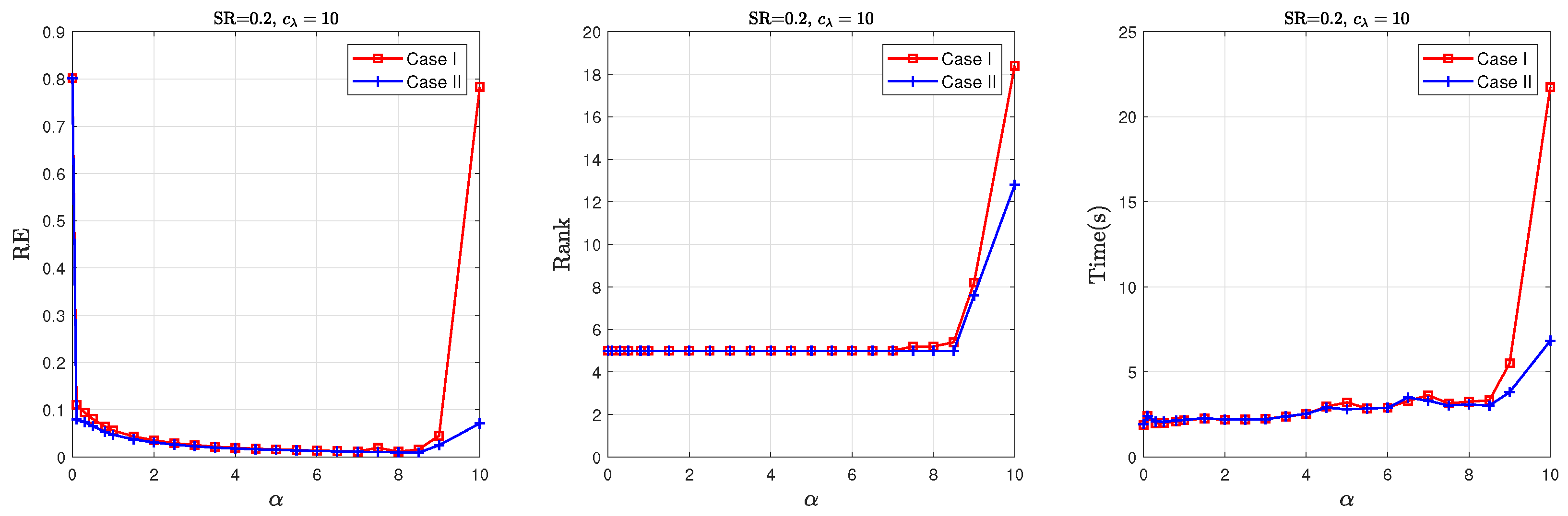
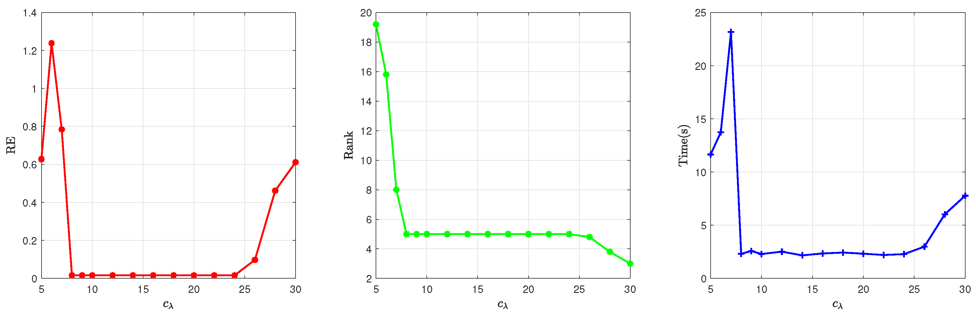
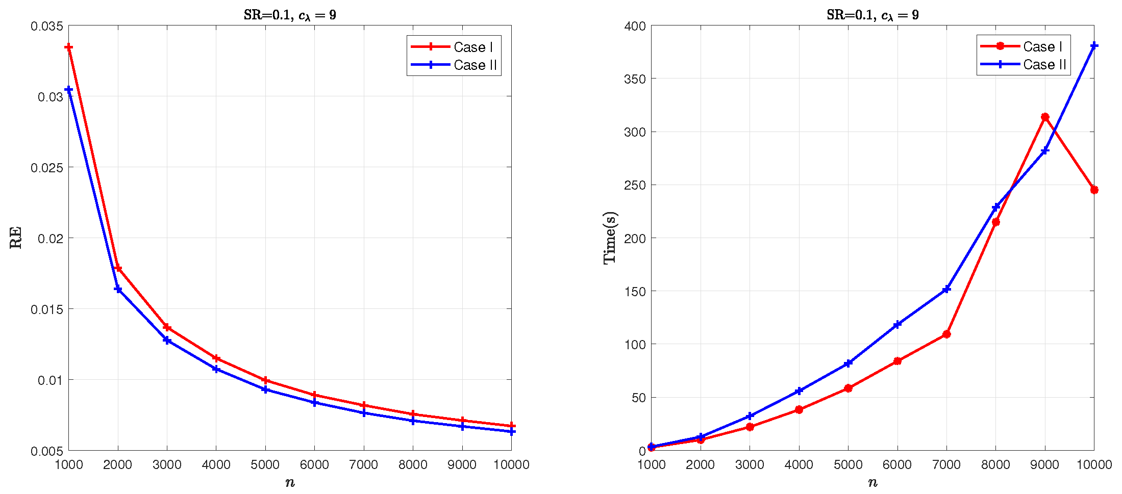
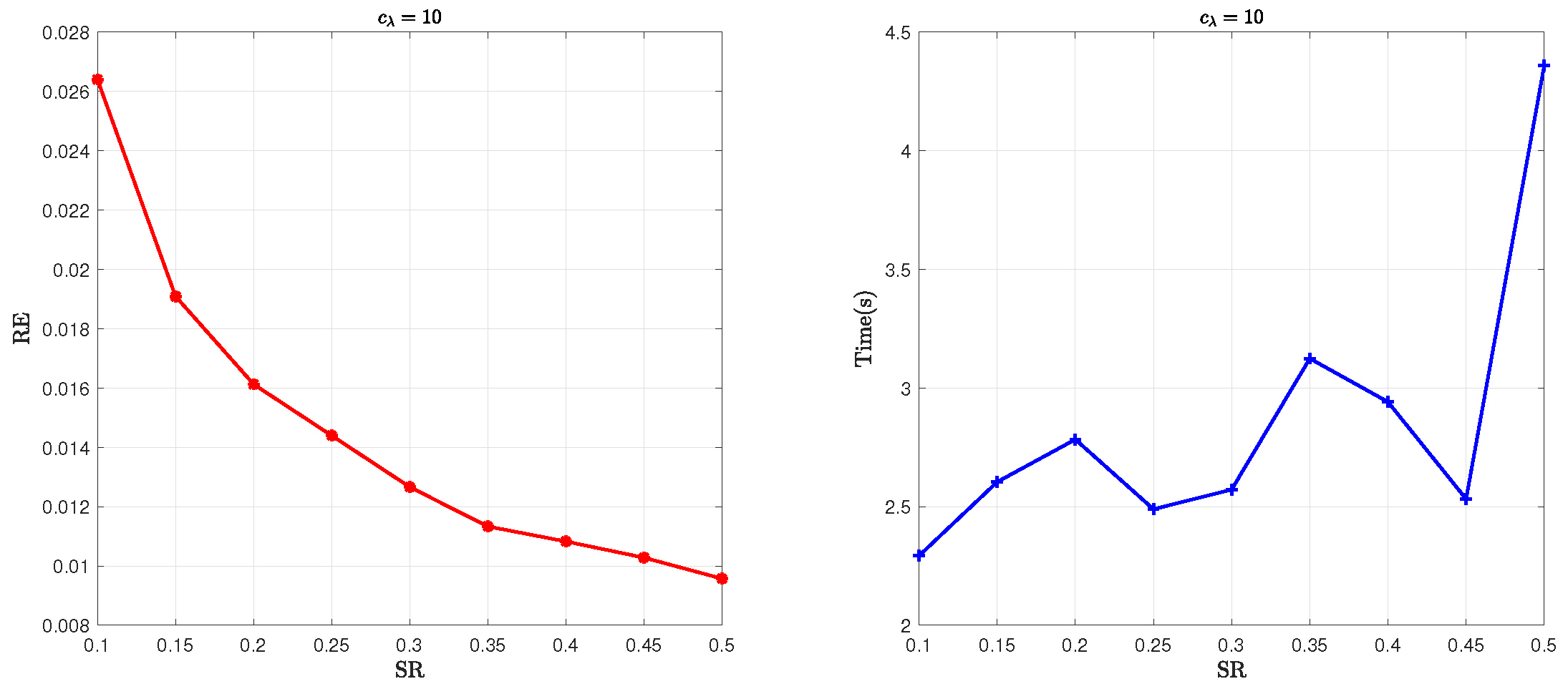
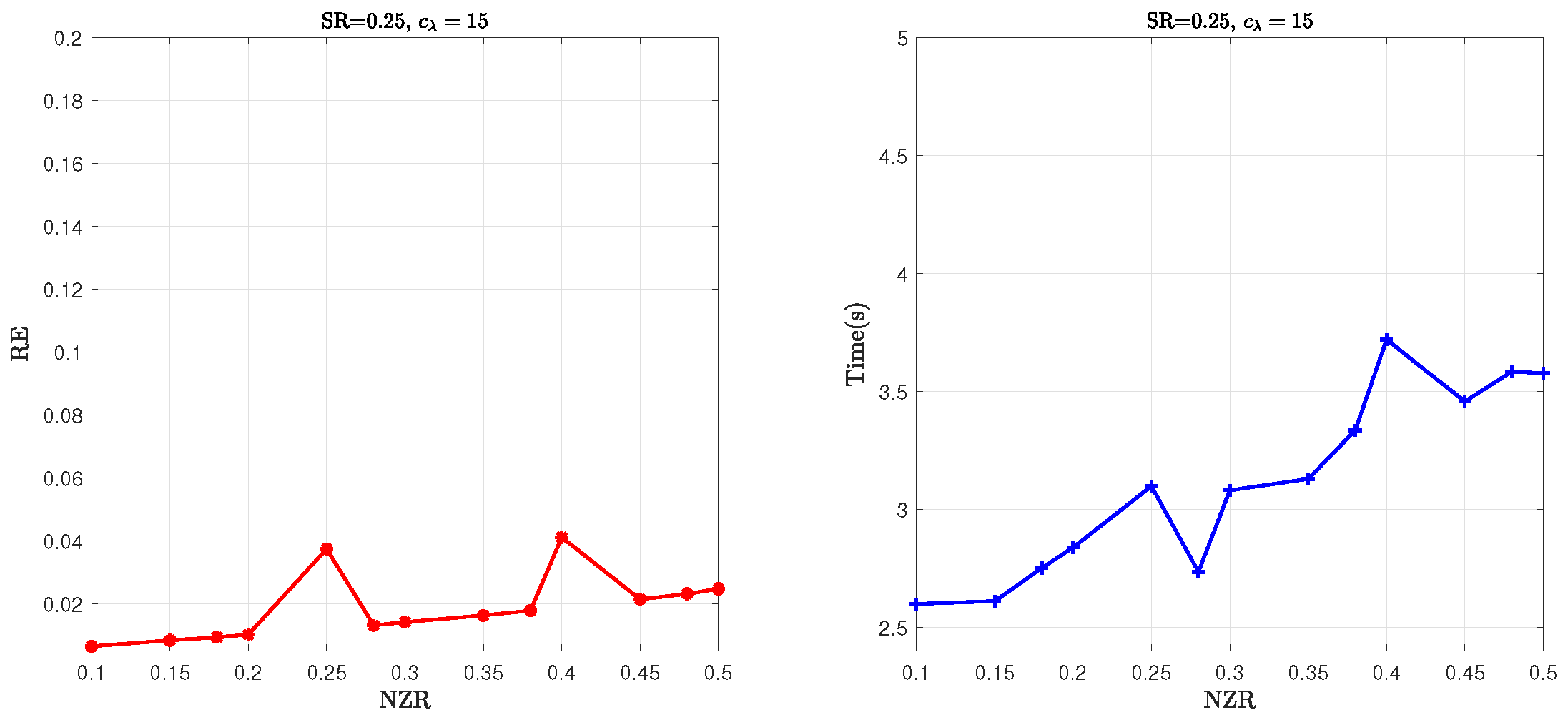
5.2. Parameter Sensitivity Analysis

In this section, the effect of the parameters on the performance of Algorithm 1 is evaluated. Figure 1 illustrates the curves of RE, recovered rank, and running time (in seconds) for Algorithm 1 when solving problem (3) with $n_1=n_2=1000$, $r^{\ast }=5$, under Case I and Case II. As shown in Figure 1, for $2\le \alpha \le 8.5$, Algorithm 1 yields both the exact rank recovery and the lowest relative error in both cases. Values of $\alpha$ exceeding 8.5 degrade the algorithm’s performance. The RE increases significantly, accompanied by an increase in computational time. In view of this, $\alpha$ is set to 5 for all subsequent experiments.

Under the settings $n_1=n_2=1000$, $r^{\ast }=5$, $\kappa =10r^{\ast }$, and $\mathrm{SR}=0.2$, Figure 2 illustrates the RE, recovered rank, and running time curves of Algorithm 1 for varying $\lambda$. The results show that a specific interval of $\lambda$ values (e.g., $8\le c_{\lambda }\le 24$) achieves low relative errors while accurately recovering the true rank of matrix $M^{\ast }$.

For $n:=n_1=n_2$ and $r^{\ast }=10$, Figure 3 shows the variation in running time and RE as n increases. These results indicate that the computational time remains below 160 s when $n\le 7000$ and does not exceed 400 s even when $n={10}^4$. With increasing n, the RE decreases rapidly, remaining below $0.015$ for $n\ge 3000$.

For Figure 4 and Figure 5, the settings are $n_1=n_2=$ 1000 and $r^{\ast }=5$. Figure 4 displays the average RE across five repetitions for sampling ratios or $\mathrm{SRs}=\{0.1,0.15,0.2,\dots ,0.5\}$. Under uniform sampling, the RE decreases monotonically with increasing SR, while the running time consistently stays within 5 s.

In Figure 5, the variation in RE with the ratio of nonzero entries in the noise vector (NZR) is examined. NZR is set to $\{0.1,0.15,0.18,\dots ,0.5\}$. As shown in Figure 5, the RE increases accordingly with NZR, while the running time remains consistently lower than 4 s. Although the difficulty of the problem escalates as NZR increases, the RE remains close to $0.02$, even when NZR reaches $0.5$.

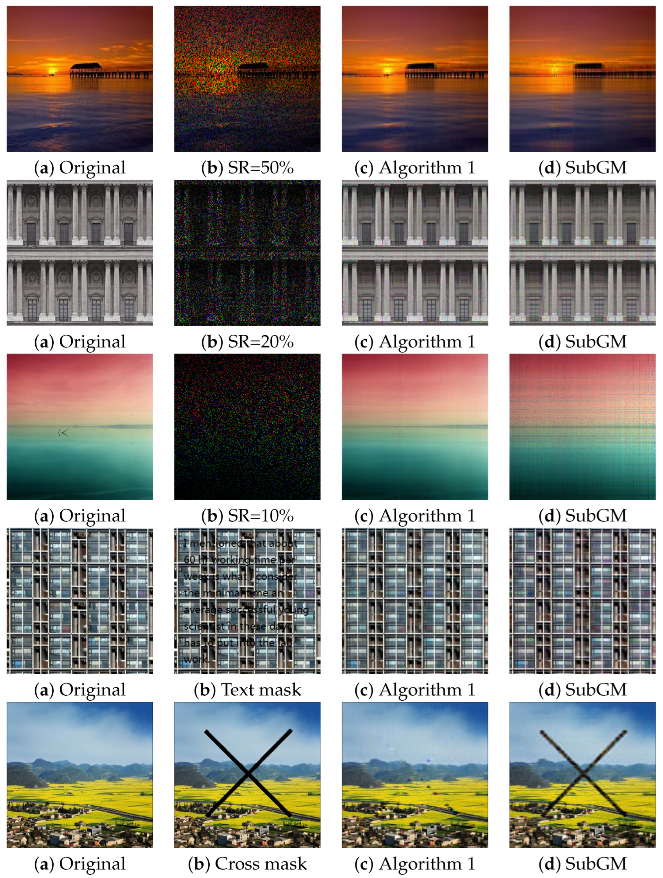
5.3. Numerical Comparisons with SubGM

The performance of Algorithm 1 in terms of solution quality and running time is compared with that of SubGM. Since the model (1) does not promote low-rank structures, $\kappa =3r^{\ast }$ and $n_1=n_2=n$ are adopted for the following tests. The numerical results of the two methods are obtained under the same stopping criterion described in Section 5.1, with ${ϵ}_1={ϵ}_2={ϵ}_3={ϵ}_4=5\times {10}^{-4}$, and $k_{\max }=500$.

Table 1. The results of the algorithm for synthetic data in Case I.

		Algorithm 1				SubGM
$\mathit{n}$	(r*, SR)	${\mathit{c}}_{\mathit{\lambda }}$	RE	Rank	Time (s)	RE	Rank	Time (s)
1000	(5, 0.10)	10	2.61 $\times {10}^{-2}$	5	1.50	1.26 $\times {10}^{-1}$	15	4.04
	(5, 0.15)	10	1.94 $\times {10}^{-2}$	5	1.48	7.71 $\times {10}^{-2}$	15	4.71
	(5, 0.20)	10	1.59 $\times {10}^{-2}$	5	1.60	6.13 $\times {10}^{-2}$	15	5.28
	(5, 0.20)	10	1.40 $\times {10}^{-2}$	5	1.73	4.93 $\times {10}^{-2}$	15	5.56
	(10, 0.10)	6	3.34 $\times {10}^{-2}$	10	1.88	2.58 $\times {10}^{-1}$	30	4.35
	(10, 0.15)	6	2.26 $\times {10}^{-2}$	10	2.88	1.38 $\times {10}^{-1}$	30	5.26
	(10, 0.20)	6	2.15 $\times {10}^{-2}$	10	2.34	8.20 $\times {10}^{-2}$	30	5.92
	(10, 0.20)	6	1.54 $\times {10}^{-2}$	10	2.33	5.88 $\times {10}^{-2}$	30	6.26
3000	(10, 0.10)	6	1.36 $\times {10}^{-2}$	10	15.0	3.61 $\times {10}^{-2}$	30	40.6
	(10, 0.15)	6	1.05 $\times {10}^{-2}$	10	17.1	2.91 $\times {10}^{-2}$	30	50.6
	(10, 0.20)	6	8.95 $\times {10}^{-3}$	10	18.3	2.23 $\times {10}^{-2}$	30	51.4
	(10, 0.20)	6	1.24 $\times {10}^{-2}$	10	20.5	2.64 $\times {10}^{-2}$	30	56.3
	(20, 0.10)	6	1.57 $\times {10}^{-2}$	20	20.3	7.73 $\times {10}^{-2}$	60	44.1
	(20, 0.15)	6	1.15 $\times {10}^{-2}$	20	20.0	3.41 $\times {10}^{-2}$	60	49.6
	(20, 0.20)	6	9.52 $\times {10}^{-3}$	20	22.4	2.42 $\times {10}^{-2}$	60	55.5
	(20, 0.20)	6	8.33 $\times {10}^{-3}$	20	23.2	2.07 $\times {10}^{-2}$	60	61.6
5000	(10, 0.10)	10	9.92 $\times {10}^{-3}$	10	45.8	2.29 $\times {10}^{-2}$	30	140.9
	(10, 0.15)	10	7.87 $\times {10}^{-3}$	10	50.0	1.93 $\times {10}^{-2}$	30	138.8
	(10, 0.20)	10	6.73 $\times {10}^{-3}$	10	46.9	1.87 $\times {10}^{-2}$	30	141.4
	(10, 0.20)	10	6.01 $\times {10}^{-3}$	10	50.1	1.61 $\times {10}^{-2}$	30	157.7
8000	(10, 0.10)	10	7.63 $\times {10}^{-3}$	10	121.3	1.53 $\times {10}^{-2}$	30	312.1
	(10, 0.15)	10	8.21 $\times {10}^{-3}$	10	140.2	1.62 $\times {10}^{-2}$	30	387.8
	(10, 0.20)	10	5.21 $\times {10}^{-3}$	10	144.9	1.40 $\times {10}^{-2}$	30	432.9
	(10, 0.20)	10	4.71 $\times {10}^{-3}$	10	154.7	1.49 $\times {10}^{-2}$	30	475.7

and

Table 2. The results of the algorithm for synthetic data in Case II.

		Algorithm 1				SubGM
$\mathit{n}$	(r*, SR)	${\mathit{c}}_{\mathit{\lambda }}$	RE	Rank	Time (s)	RE	Rank	Time (s)
1000	(5, 0.10)	10	2.42 $\times {10}^{-2}$	5	1.37	8.76 $\times {10}^{-2}$	15	3.85
	(5, 0.15)	10	1.82 $\times {10}^{-2}$	5	1.43	6.14 $\times {10}^{-2}$	15	4.81
	(5, 0.20)	10	1.49 $\times {10}^{-2}$	5	1.39	5.03 $\times {10}^{-2}$	15	5.49
	(5, 0.20)	10	1.31 $\times {10}^{-2}$	5	1.28	4.61 $\times {10}^{-2}$	15	5.70
1000	(10, 0.10)	6	3.00 $\times {10}^{-2}$	10	1.86	1.85 $\times {10}^{-1}$	30	4.31
	(10, 0.15)	6	2.07 $\times {10}^{-2}$	10	1.88	9.23 $\times {10}^{-2}$	30	4.26
	(10, 0.20)	6	1.65 $\times {10}^{-2}$	10	2.24	6.02 $\times {10}^{-2}$	30	5.92
	(10, 0.20)	6	1.42 $\times {10}^{-2}$	10	2.28	4.71 $\times {10}^{-2}$	30	6.26
3000	(10, 0.10)	6	1.27 $\times {10}^{-2}$	10	15.5	3.11 $\times {10}^{-1}$	30	40.6
	(10, 0.15)	6	9.85 $\times {10}^{-3}$	10	16.1	2.71 $\times {10}^{-2}$	30	45.6
	(10, 0.20)	6	8.33 $\times {10}^{-3}$	10	17.3	2.27 $\times {10}^{-2}$	30	50.4
	(10, 0.20)	6	7.40 $\times {10}^{-3}$	10	18.5	2.11 $\times {10}^{-2}$	30	55.3
3000	(20, 0.10)	6	1.44 $\times {10}^{-2}$	20	20.3	5.30 $\times {10}^{-2}$	60	44.1
	(20, 0.15)	6	1.07 $\times {10}^{-2}$	20	22.0	2.79 $\times {10}^{-2}$	60	49.6
	(20, 0.20)	6	8.82 $\times {10}^{-3}$	20	22.4	2.11 $\times {10}^{-2}$	60	54.5
	(20, 0.20)	6	7.73 $\times {10}^{-3}$	20	23.2	1.85 $\times {10}^{-2}$	60	59.6
5000	(10, 0.10)	10	9.29 $\times {10}^{-3}$	10	40.8	2.07 $\times {10}^{-2}$	30	110.9
	(10, 0.15)	10	7.37 $\times {10}^{-3}$	10	48.0	1.84 $\times {10}^{-2}$	30	126.8
	(10, 0.20)	10	6.29 $\times {10}^{-3}$	10	46.9	1.75 $\times {10}^{-2}$	30	141.4
	(10, 0.20)	10	5.62 $\times {10}^{-3}$	10	50.1	1.61 $\times {10}^{-2}$	30	156.7
8000	(10, 0.10)	10	7.13 $\times {10}^{-3}$	10	99.3	1.51 $\times {10}^{-2}$	30	283.1
	(10, 0.15)	10	5.71 $\times {10}^{-3}$	10	114.2	1.56 $\times {10}^{-2}$	30	337.8
	(10, 0.20)	10	4.91 $\times {10}^{-3}$	10	114.9	1.50 $\times {10}^{-2}$	30	353.9
	(10, 0.20)	10	4.38 $\times {10}^{-3}$	10	124.7	1.48 $\times {10}^{-2}$	30	395.7

report the average results across five randomly generated instances for each setting. Compared with SubGM, Algorithm 1 consistently achieves the lowest RE in significantly less computational time.

Reconstructing images from limited and noisy measurements is a key application of low-rank matrix completion. To further evaluate the effectiveness of the proposed method, experiments were conducted on images from the ZJU dataset [19]. Each image has dimensions of $300\times 300$. The initial points for both algorithms were obtained using the same procedure described in Section 5.1, with $\kappa =40$.

The results are presented in

Table 3. Summary of experimental results of image recovery.

	Algorithm	RE	PSNR	Time (s)
Sampling Ratio = 50%	Algorithm 1	0.0708	30.57	1.72
	SubGM	0.0991	27.82	2.60
Sampling Ratio = 20%	Algorithm 1	0.1178	24.22	0.76
	SubGM	0.1361	23.07	1.84
Sampling Ratio = 10%	Algorithm 1	0.0369	33.61	0.59
	SubGM	0.1113	24.06	1.49
Image with text mask	Algorithm 1	0.1639	21.10	0.48
	SubGM	0.1700	20.82	4.84
Image with cross mask	Algorithm 1	0.0934	16.71	1.34
	SubGM	0.1811	7.40	5.67

and Figure 6. The images were undersampled using various sampling rates and masks and then restored using a similar process reported in [9]. Table 3 lists the relative error and peak signal-to-noise ratio (PSNR) for each image restoration task. The results show that the proposed algorithm outperforms SubGM in terms of both computational time and restoration quality.

6. Conclusions

This paper has focused on robust factorization models for low-rank matrix recovery, which are of great significance in multiple fields such as machine learning and imaging sciences. To deal with the challenge of outliers, an ${\ell }_1$-loss robust factorized model with ${\ell }_{2,0}$-norm regularization is proposed. Given the nonconvex and discontinuous nature of the problem, an approximation problem (3) is constructed. Under mild assumptions, the equivalence of stationary points between the original and the approximation problems is verified, and it is proven that the global optimum of the approximation problem can serve as an approximate optimal solution for the original problem in terms of objective value. On top of that, a fast PALM method is proposed to solve the approximation problem, and the global convergence of the iterate sequence is established. The numerical experiments on synthetic datasets with outliers and image restoration tasks demonstrate that the PALM method achieves low relative errors within a significantly shorter computational time, particularly when dealing with large-scale datasets. Despite the promising results of the proposed approach, there are some limitations. The performance of the algorithm relies on the proper selection of parameters such as $\lambda$ and $\alpha$. To address these limitations, future research works will include the development of adaptive parameter-tuning strategies.

References

1. Candès, E.J.; Recht, B. Exact matrix completion via convex optimization. Found. Comput. Math. 2009, 9, 717–772. [Google Scholar] [CrossRef]
2. Davenport, M.A.; Romberg, J. An overview of low-rank matrix recovery from incomplete observations. IEEE J. Sel. Top. Signal Process. 2016, 10, 608–622. [Google Scholar] [CrossRef]
3. Fazel, M.; Hindi, H.; Boyd, S. Rank Minimization and Applications in System Theory. Proc. 2004 Am. Control Conf. 2004, 4, 3273–3278. [Google Scholar]
4. Gross, D.; Liu, Y.K.; Flammia, S.T.; Becker, S.; Eisert, J. Quantum state tomography via compressed sensing. Phys. Rev. Lett. 2010, 105, 150401. [Google Scholar] [CrossRef] [PubMed]
5. Negahban, S.; Wainwright, M.J. Estimation of (near) low-rank matrices with noise and high-dimensional scaling. Ann. Stat. 2011, 39, 1069–1097. [Google Scholar] [CrossRef]
6. Charisopoulos, V.; Chen, Y.; Davis, D.; Díaz, M.; Ding, L.; Drusvyatskiy, D. Low-Rank Matrix Recovery with Composite Optimization: Good Conditioning and Rapid Convergence. Found. Comput. Math. 2021, 21, 1505–1593. [Google Scholar] [CrossRef]
7. Li, X.; Zhu, Z.H.; So, A.M.; Vidal, R. Nonconvex Robust Low-Rank Matrix Recovery. SIAM J. Optim. 2020, 30, 660–686. [Google Scholar] [CrossRef]
8. Ma, J.H.; Fattahi, S. Global Convergence of Sub-gradient Method for Robust Matrix Recovery: Small Initialization, Noisy Measurements, and Over-parameterization. J. Mach. Learn. Res. 2023, 24, 1–84. [Google Scholar]
9. Wang, Z.Y.; So, H.C.; Liu, Z.F. Fast and robust rank-one matrix completion via maximum correntropy criterion and half-quadratic optimization. Signal Process. 2022, 198, 108580. [Google Scholar] [CrossRef]
10. Tao, T.; Qian, Y.T.; Pan, S.H. Column 2,0-norm regularized factorization model of low-rank matrix recovery and its computation. SIAM J. Optim. 2022, 32, 959–988. [Google Scholar] [CrossRef]
11. Candès, E.J.; Li, X.; Ma, Y.; Wright, J. Robust principal component analysis. J. ACM 2011, 11, 1–37. [Google Scholar] [CrossRef]
12. Josz, C.; Ouyang, Y.; Zhang, R.; Lavaei, J.; Sojoudi, S. A theory on the absence of spurious solutions for nonconvex and nonsmooth optimization. Adv. Neural Inf. Process. Syst. 2018, 31, 2441–2449. [Google Scholar]
13. Li, Y.; Sun, Y.; Chi, Y. Low-rank positive semidefinite matrix recovery from corrupted rank-one measurements. IEEE Trans. Signal Process. 2017, 65, 397–408. [Google Scholar] [CrossRef]
14. Rockafellar, R.T.; Wets, R.J.-B. Variational Analysis; Springer: Berlin/Heidelberg, Germany, 1998. [Google Scholar]
15. Attouch, H.; Bolte, J.; Redont, P.; Soubeyran, A. Proximal alternating minimization and projection methods for nonconvex problems: An approach based on the Kurdyka-Łojasiewicz inequality. Math. Oper. Res. 2010, 35, 438–457. [Google Scholar] [CrossRef]
16. Nocedal, J.; Wright, S.J. Numerical Optimization; Springer: Berlin/Heidelberg, Germany, 2000. [Google Scholar]
17. Bolte, J.; Sabach, S.; Teboulle, M. Proximal alternating linearized minimization for nonconvex and nonsmooth problems. Math. Program. 2014, 146, 459–494. [Google Scholar] [CrossRef]
18. Polyak, B.T. Minimization of unsmooth functions. USSR Comput. Math. Math. Phys. 1969, 9, 14–29. [Google Scholar] [CrossRef]
19. Hu, Y.; Zhang, D.; Ye, J.; Li, X.; He, X. Fast and accurate matrix completion via truncated nuclear norm regularization. IEEE Trans. Pattern Anal. Mach. Intell. 2012, 35, 2117–2130. [Google Scholar] [CrossRef] [PubMed]
Figure 1. Curves of RE, rank, and running time of Algorithm 1 with different α values.
Mathematics 13 01466 g001
Figure 2. Curves of relative error, rank, and running time of Algorithm 1 in Case I.
Mathematics 13 01466 g002
Figure 3. RE and running time curves of Algorithm 1 in Case I–II with different values of n.
Mathematics 13 01466 g003
Figure 4. RE and running time curves of Algorithm 1 in Case I with different SRs.
Mathematics 13 01466 g004
Figure 5. RE and running time curves of Algorithm 1 in Case I with different NZRs.
Mathematics 13 01466 g005
Figure 6. Experimental results of image recovery.
Mathematics 13 01466 g006