
SG-ResNet: Spatially Adaptive Gabor Residual Networks with Density-Peak Guidance for Joint Image Steganalysis and Payload Location


Abstract
1. Introduction
- (1)
- The adaptive density-peak Gabor module extracts steganographic features by combining multi-scale textures with density-based filters, capturing subtle embedding artifacts in both spatial and frequency domains.
- (2)
- The three-channel fused tickling nonlinear truncated module enhances critical feature sensitivity and amplifies hidden residuals in steganographic regions, increasing the accuracy by 11.2%.
- (3)
- The multilevel feedback residual architecture achieves state-leading hidden secret reconstruction with PSNR of 29, outperforming existing models by 15%.
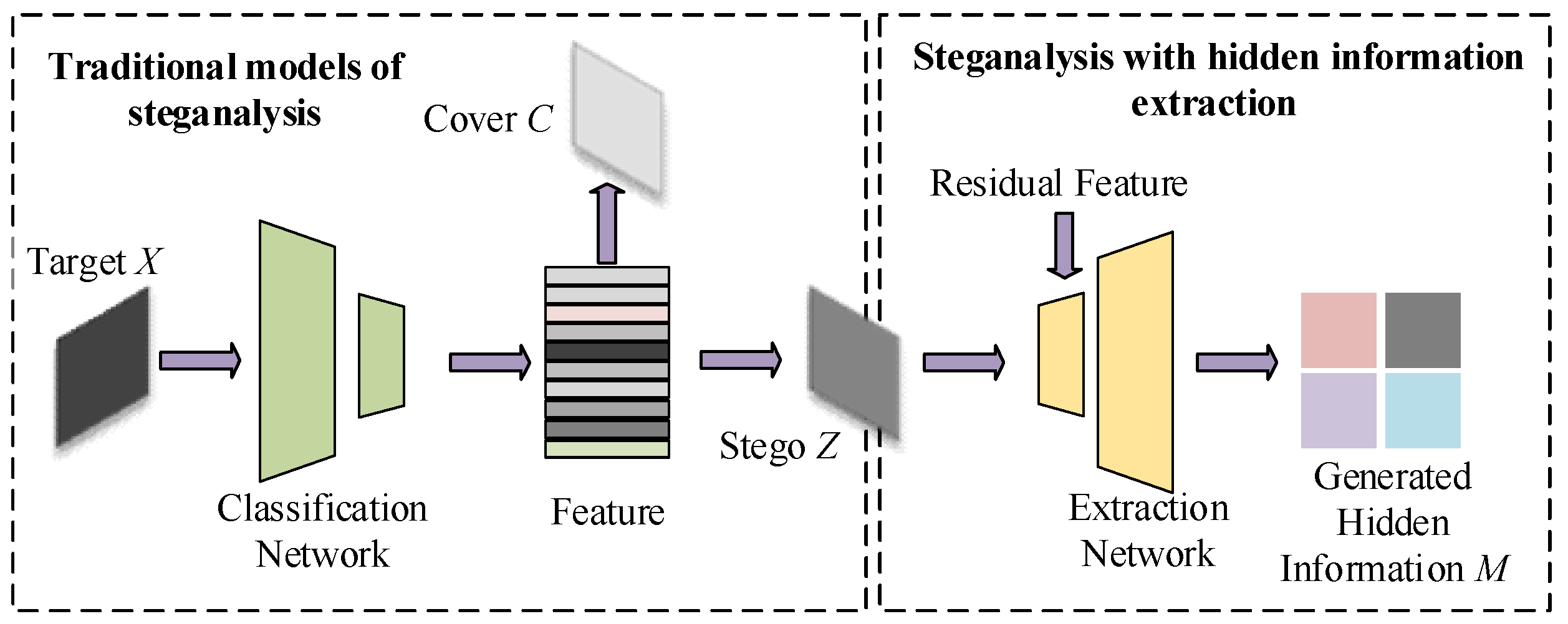
2. Related Concepts and Works
2.1. Related Concepts
2.2. Existing Steganographic Information Location Works
2.3. Evaluation Indexes
3. Proposed Steganalysis Framework
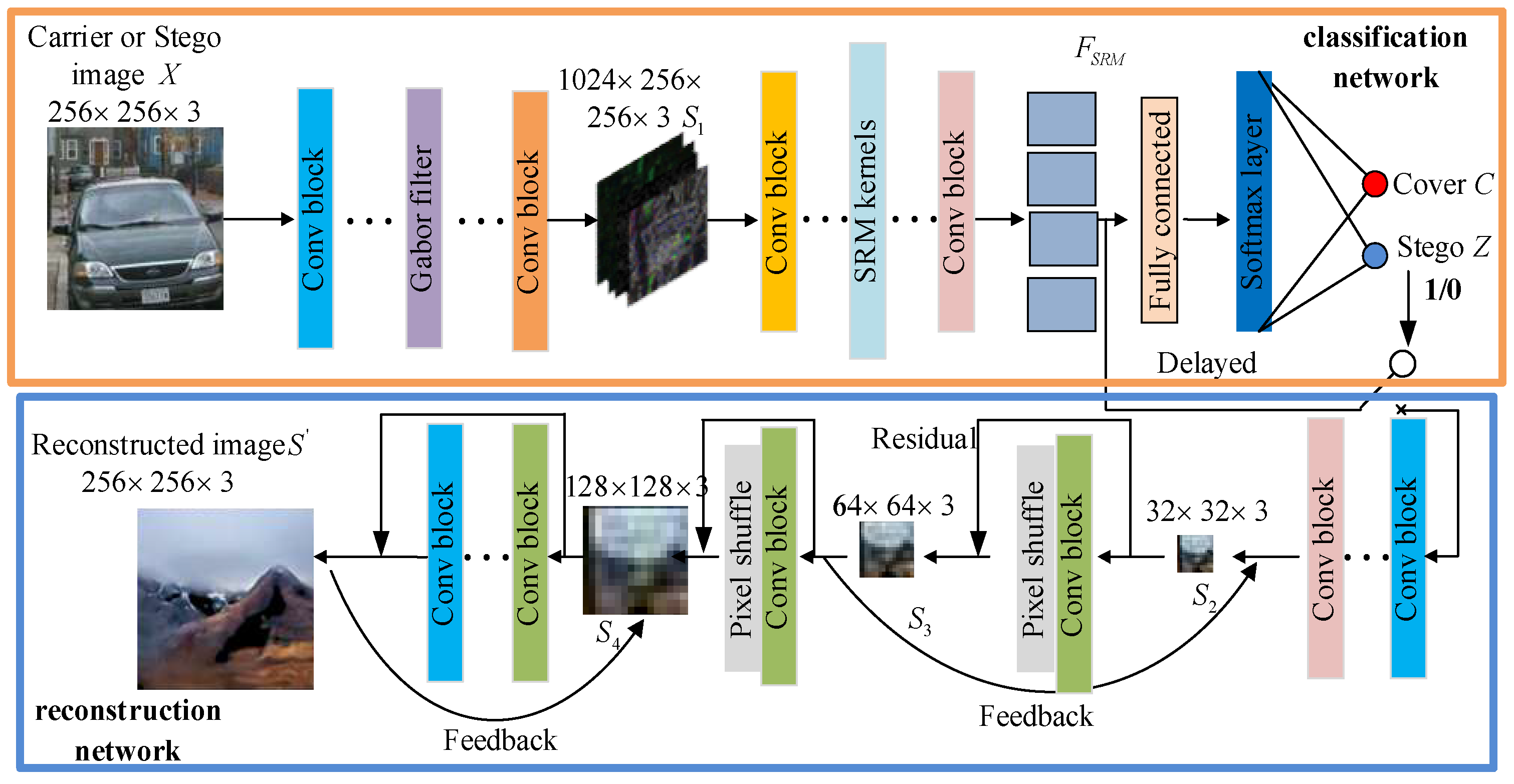
3.1. SG-ResNet Model
3.2. Classification Framework for Hidden Information
3.2.1. Details of the Classification Network
3.2.2. Adaptive Density Peak Gabor Convolution Block and
3.3. Tickling Nonlinear Truncated Steganalyzer, TSRM
3.4. Reconstruction Framework for Hidden Information
| Algorithm 1: SG-ResNet for Image Steganalysis and Hidden-Message Reconstruction | ||
| Input: Training dataset , stego image , label , supervisory matrix of residual feature , Sample size N. Hyperparameter: ; ; SG-ResNet initial parameters, (learning rate, loss weight, training batch size (T), etc.). | ||
| Output: trained parameters, ; extracted secret information, . | ||
| 1 ; 2 do 3 4 5 | ||
| 6 7 8 Supervised matrix guidance for feature learning 9 10 DPC feature selection 11 | ||
| 12 | ||
| 13 | ||
| 14 | ||
| 15 | ||
| 16 | ||
| 17 | ||
| 18 | ||
| 19 | ||
| 20 | ||
| 21 | ||
| 22 | ||
| 23 24 |
Return | |
| 25 26 | Steganalysis prediction | |
| 27 28 |
| |
| 29 | ||
| 30 | ||
| 31 | ||
| 32 | ||
| 33 | ||
| 34 Return | ||
4. Experimental Results and Discussion
4.1. Datasets and Training Settings
4.2. Result Analysis
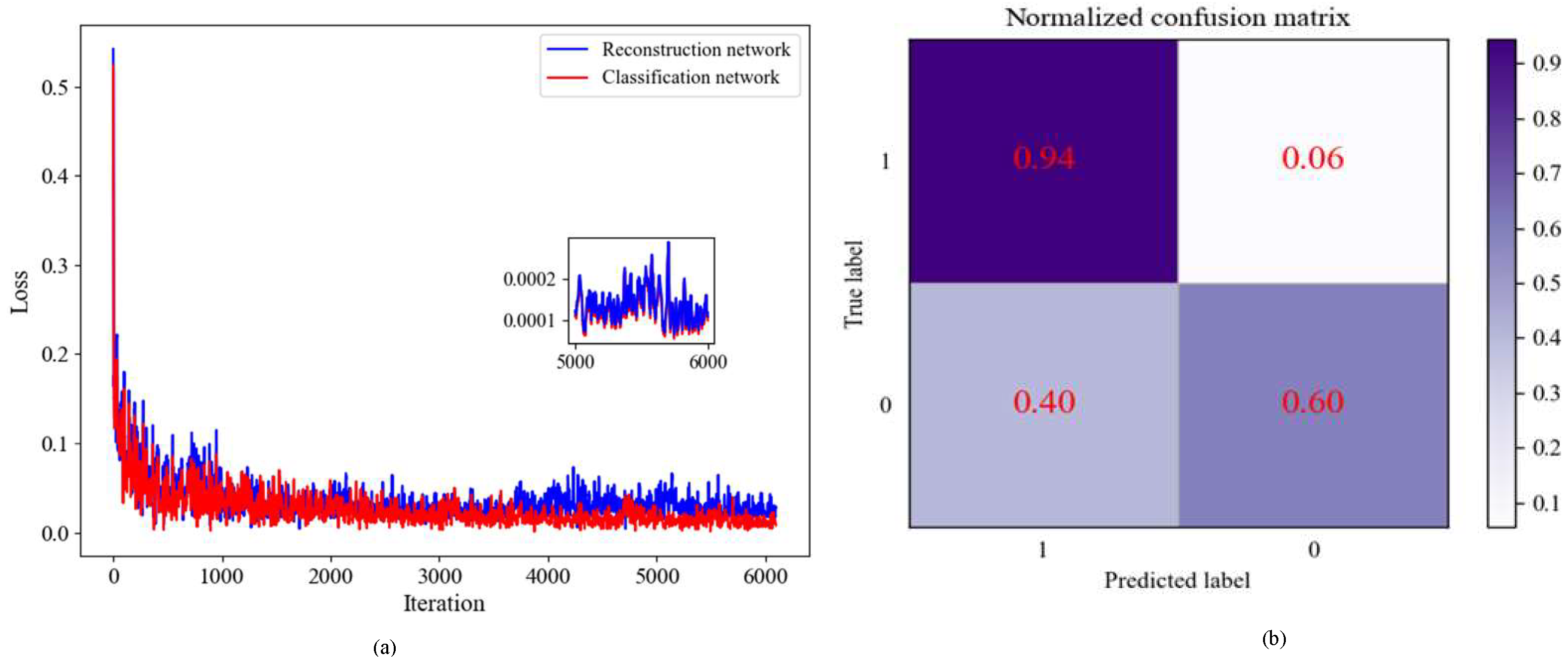
4.2.1. Performance Evaluation Against Conventional Steganography
- (1)
- Steganographic Image Detection and Classification
- (2)
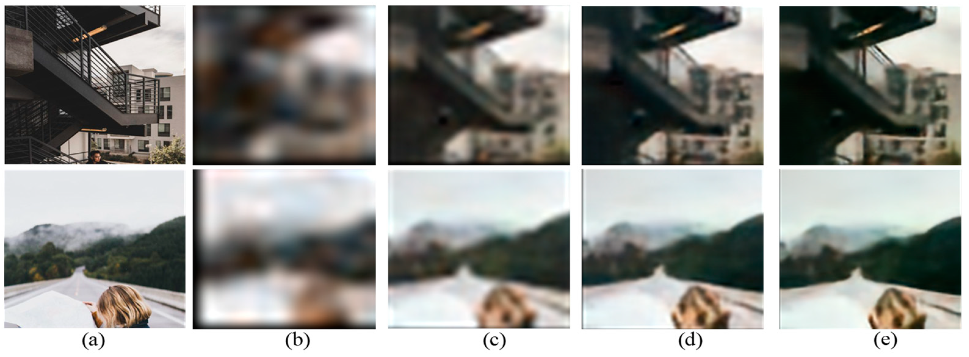
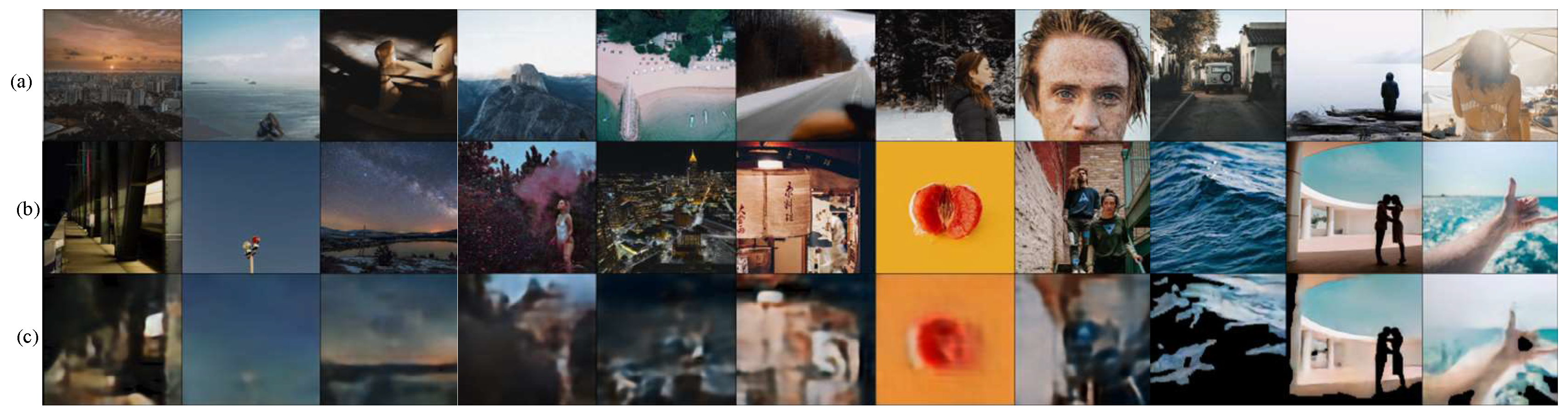
- Embedded Information Localization and Extraction
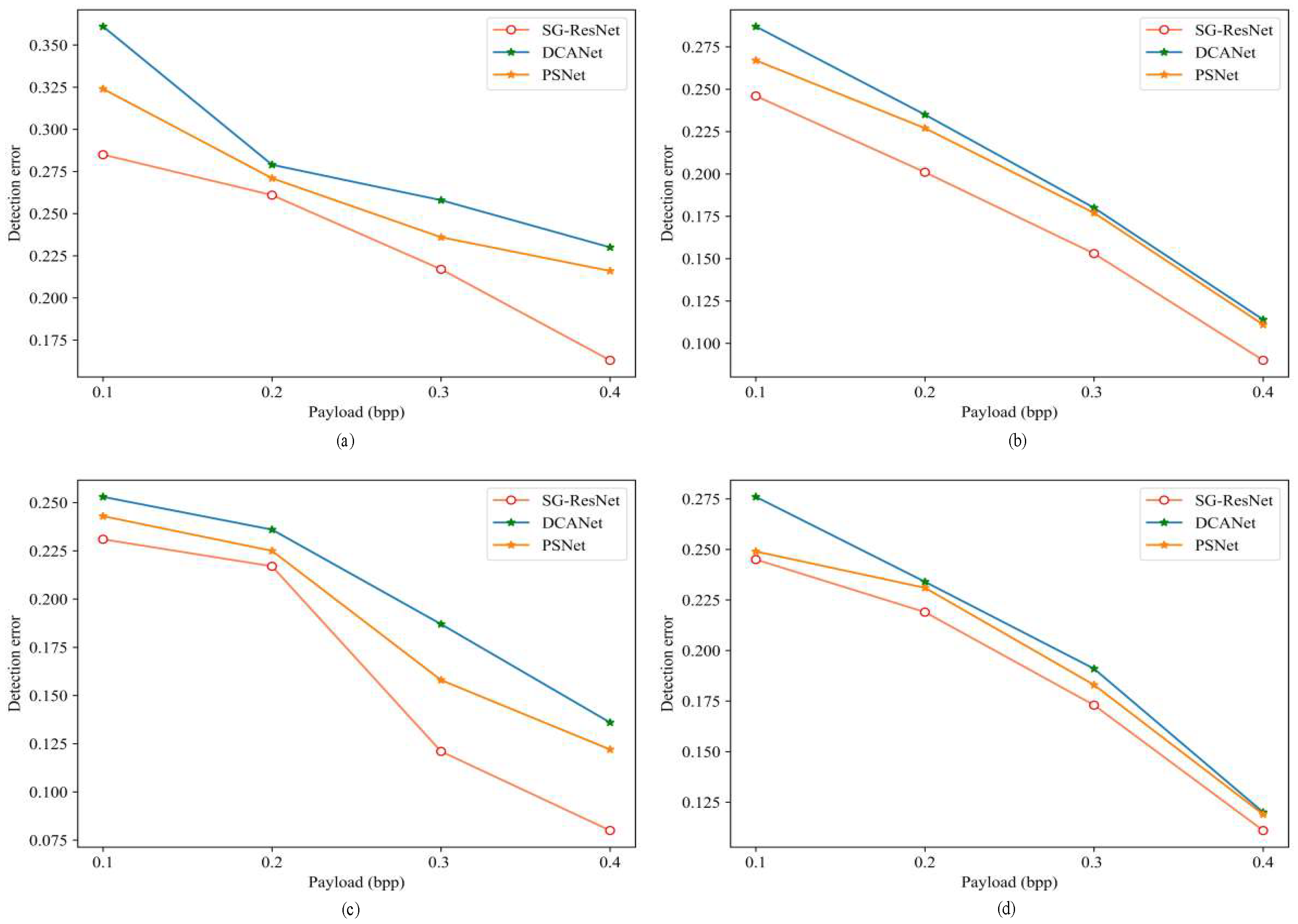
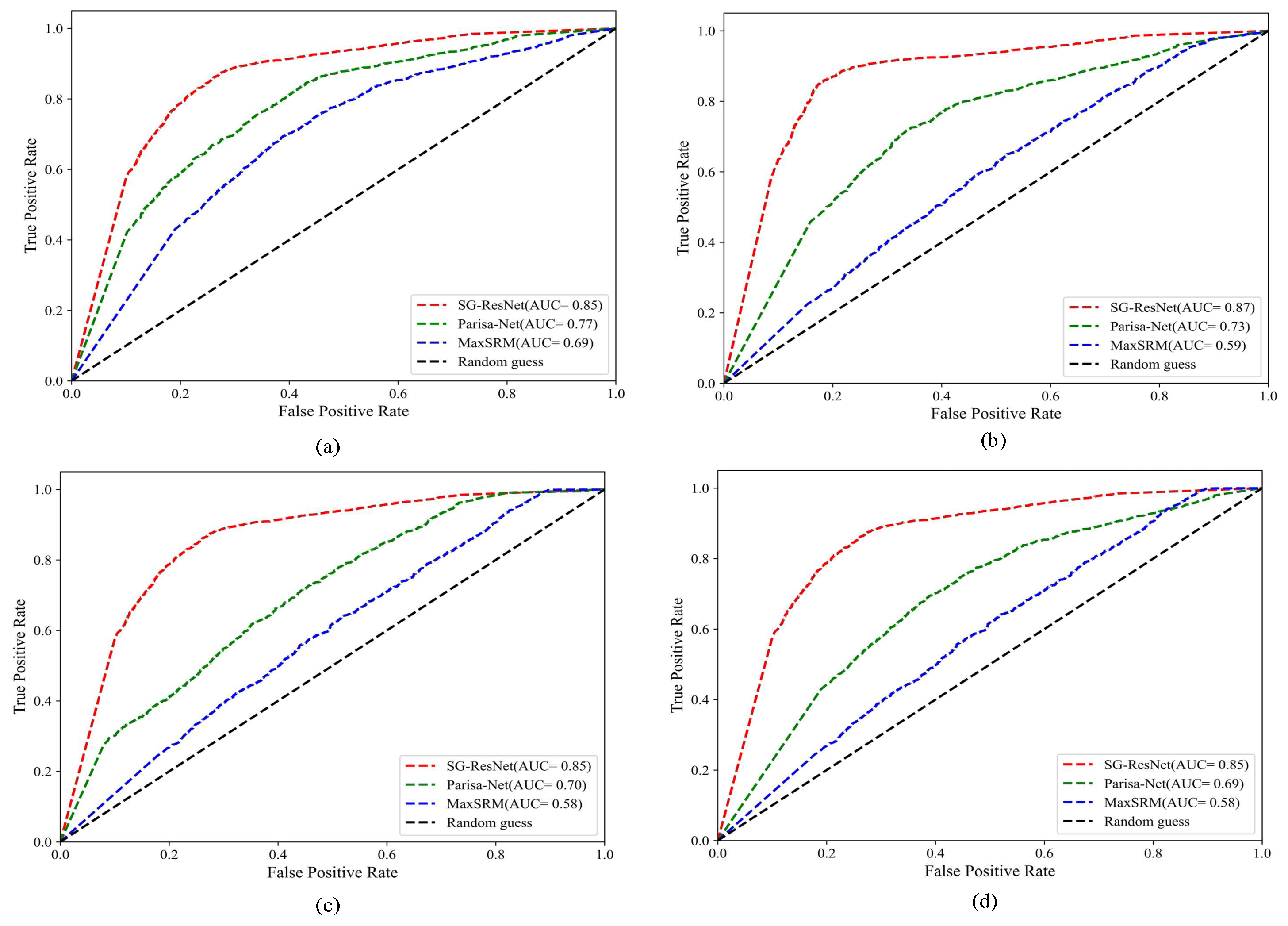
4.2.2. Performance Evaluation Against Deep Learning-Based Steganography
- (1)
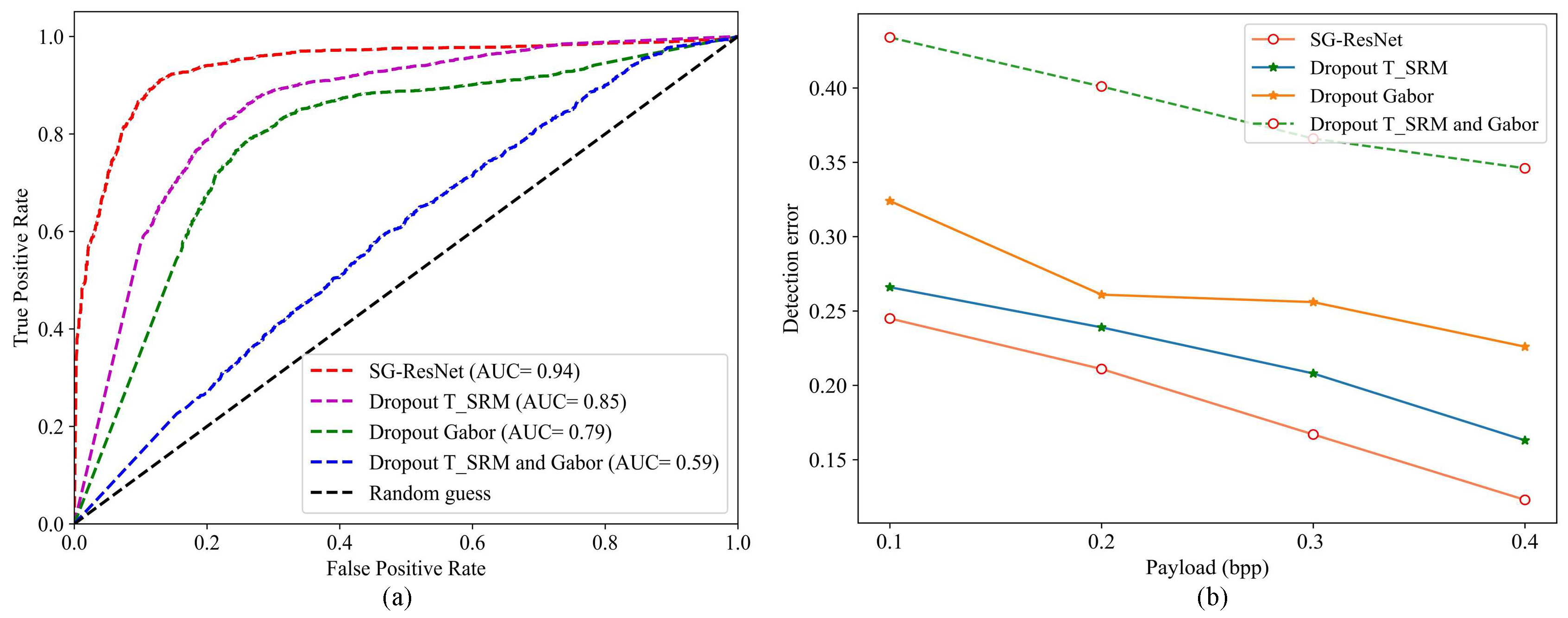
- Steganographic Image Detection and Classification
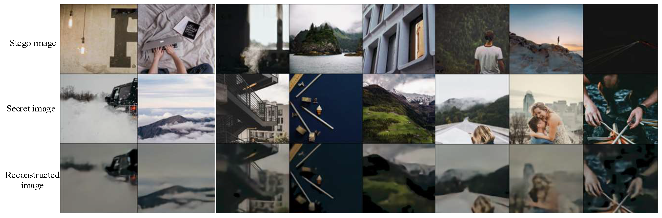
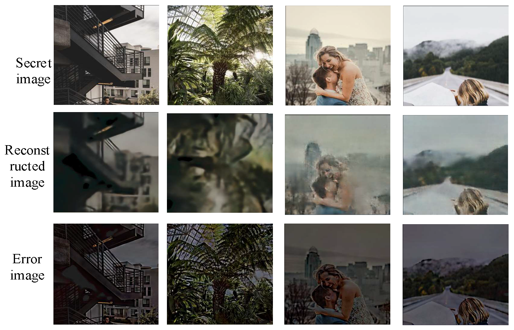
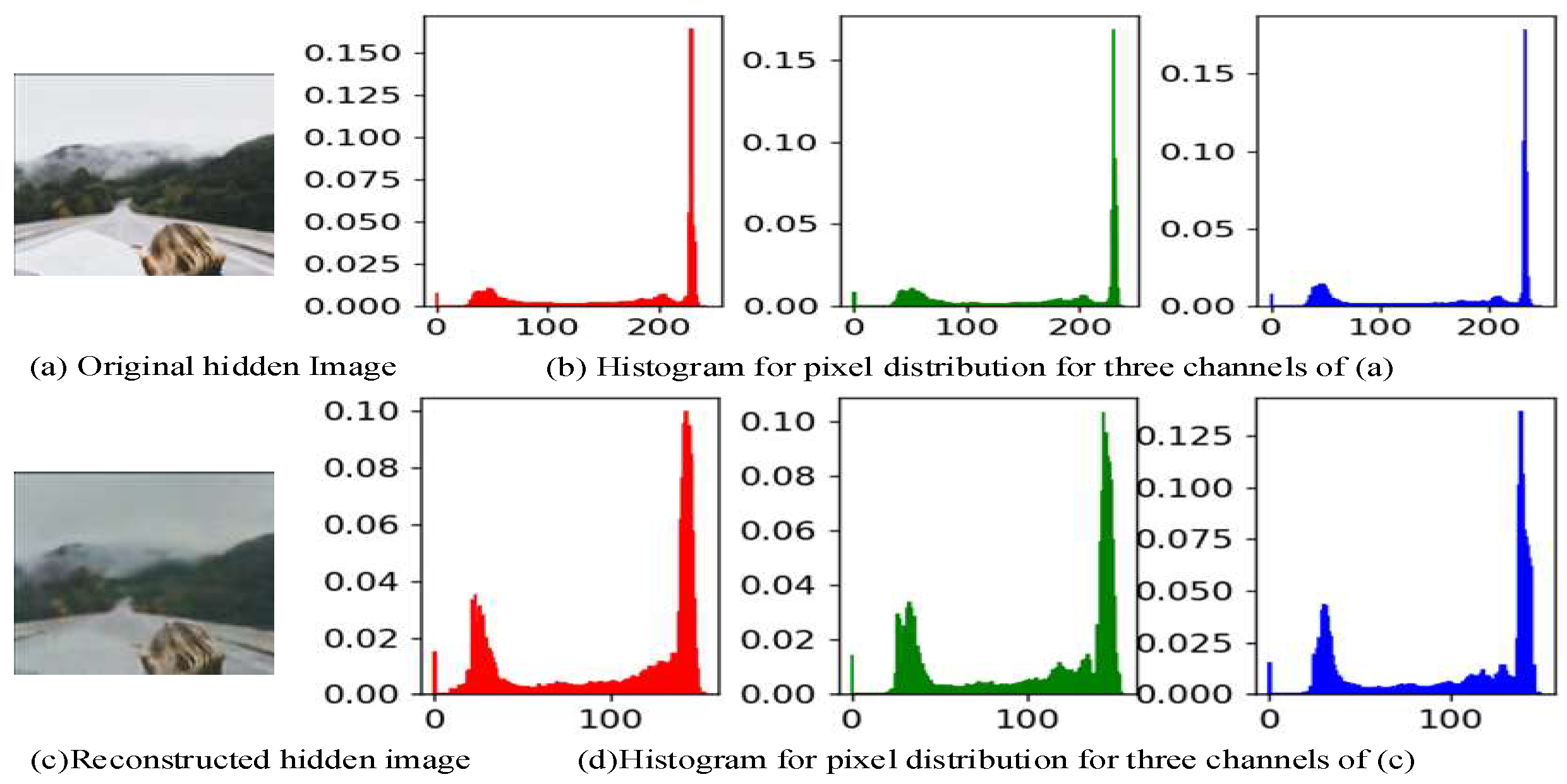
- (2)
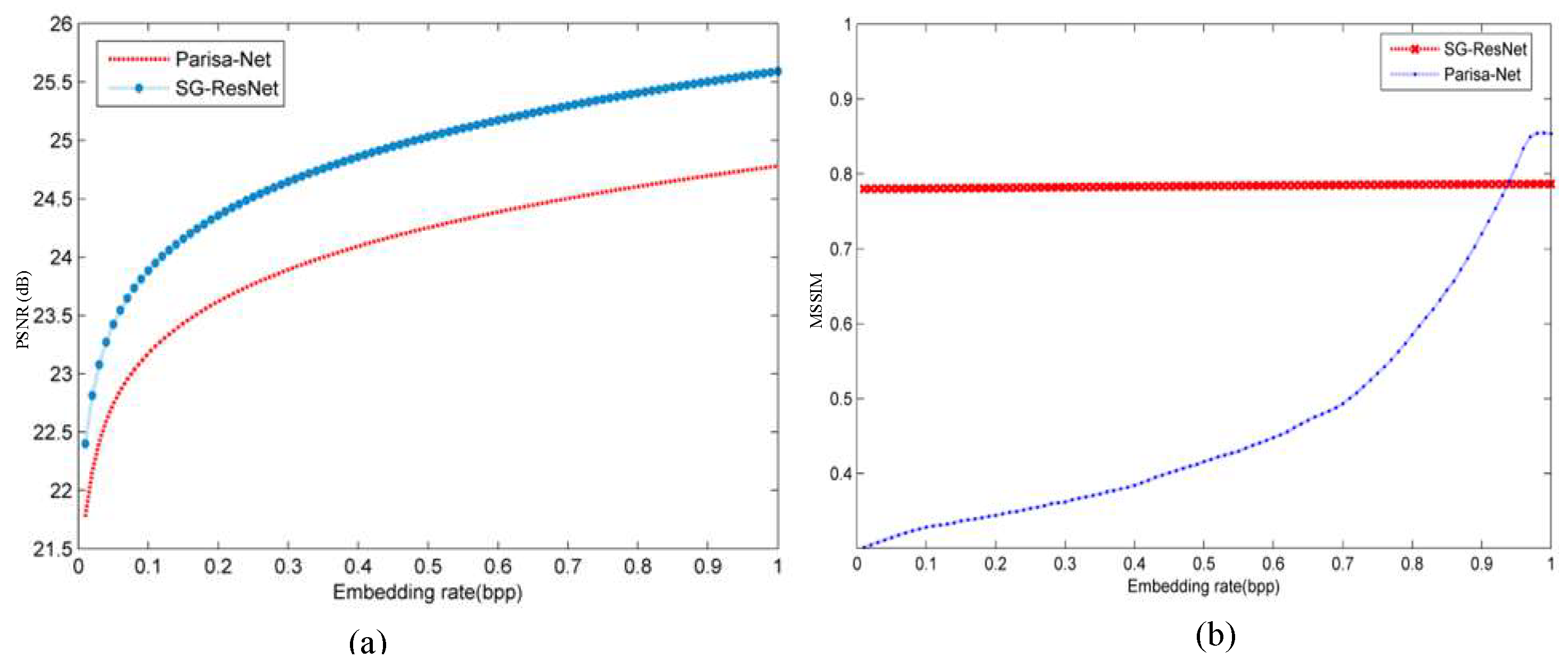
- Embedded Information Localization and Extraction
4.3. Feature Extraction Capability Analysis
4.4. Ablation Experiment
4.4.1. Module Ablation
4.4.2. Hyperparameter Analysis
4.5. Robustness and Parameter Sensitivity Analysis
4.5.1. Noise, Cropping, and Compression Attack
4.5.2. Performance Across Datasets
5. Conclusions
Author Contributions
Funding
Data Availability Statement
Conflicts of Interest
References
- Kumar, S.; Kumar, D.; Dangi, R.; Choudhary, G.; Dragoni, N.; You, I. A review of lightweight security and privacy for resource-constrained IoT devices. Cmc-Comput. Mater. Con. 2024, 78, 31–63. [Google Scholar] [CrossRef]
- Luo, J.; He, P.S.; Liu, J.Y.; Wang, H.X.; Wu, C.W.; Zhou, S.L. Reversible adversarial steganography for security enhancement. J. Vis. Commun. Image Represent. 2023, 97, 103935. [Google Scholar] [CrossRef]
- Ahanger, T.A.; Ullah, I.; Algamdi, S.A.; Tariq, U. Machine learning-inspired intrusion detection system for IoT: Security issues and future challenges. Comput. Electr. Eng. 2025, 123, 110265. [Google Scholar] [CrossRef]
- Prabhu, D.; Vijay, B.S.; Suthir, S. Privacy preserving steganography-based biometric authentication system for cloud computing environment. Meas. Sens. 2024, 24, 100511. [Google Scholar] [CrossRef]
- Alaaldin, D.; Yassine, B. Enhancing the performance of convolutional neural network image-based steganalysis in spatial domain using spatial rich model and 2D Gabor filters. J. Inf. Secur. Appl. 2024, 85, 103864. [Google Scholar]
- Fridrich, J.; Kodovsky, J. Rich models for steganalysis of digital images. IEEE Trans. Inf. Foren. Sec. 2012, 7, 868–882. [Google Scholar] [CrossRef]
- Gupta, A.; Chhikara, R.; Sharma, P. Feature reduction of rich features for universal steganalysis using a metaheuristic approach. Int. J. Comput. Sci. Eng. 2022, 25, 211–221. [Google Scholar] [CrossRef]
- Jia, J.; Luo, M.; Ma, S.; Wang, L.; Liu, Y. Consensus-clustering-based automatic distribution matching for cross-domain image steganalysis. IEEE Trans. Knowl. Data Eng. 2023, 35, 5665–5679. [Google Scholar] [CrossRef]
- Xue, Y.M.; Wu, J.X.; Ji, R.H.; Zhong, P.; Wen, J.; Peng, W.L. Adaptive domain-invariant feature extraction for cross-domain linguistic steganalysis. IEEE Trans. Inf. Foren. Sec. 2024, 19, 920–933. [Google Scholar] [CrossRef]
- Mohamed, N.; Rabie, T.; Kamel, I. A review of color image steganalysis in the transform domain. In Proceedings of the 14th International Conference on Innovations in Information Technology, Al Ain, United Arab Emirates, 17–18 November 2020; pp. 17–18. [Google Scholar]
- Arivazhagan, S.; Amrutha, E.; Jebarani, W.S. Universal steganalysis of spatial content-independent and content-adaptive steganographic algorithms using normalized feature derived from empirical mode decomposed components. Signal Process. Image 2022, 101, 116567. [Google Scholar] [CrossRef]
- Dalal, M.; Juneja, M. Steganalysis of DWT-based steganography technique for SD and HD videos. Wireless Pers. Commun. 2023, 128, 2441–2452. [Google Scholar] [CrossRef]
- Qiao, T.; Luo, X.; Wu, T.; Xu, M.; Qian, Z. Adaptive steganalysis based on statistical model of quantized DCT coefficients for JPEG images. IEEE Trans. Dependable Secur. Comput. 2021, 18, 2736–2751. [Google Scholar] [CrossRef]
- Pan, Y.; Ni, J. Domain transformation of distortion costs for efficient JPEG steganography with symmetric embedding. Symmetry 2024, 16, 575. [Google Scholar] [CrossRef]
- Weng, S.; Sun, S.; Yu, L. Fast SWT-based deep steganalysis network for arbitrary-sized images. IEEE Signal Process. Lett. 2023, 30, 1782–1786. [Google Scholar] [CrossRef]
- Liu, X.; Li, W.; Lin, K.; Li, B. Spatial-frequency feature fusion network for lightweight and arbitrary-sized JPEG steganalysis. IEEE Signal Process. Lett. 2024, 31, 2585–2589. [Google Scholar] [CrossRef]
- Deng, S.N.; Wu, L.F.; Shi, G.; Xing, L.H.; Jian, M.; Xiang, Y.; Dong, R.H. Learning to compose diversified prompts for image emotion classification. Comput. Vis. Media 2024, 10, 1169–1183. [Google Scholar] [CrossRef]
- Shi, G.; Deng, S.N.; Wang, B.; Feng, C.; Zhuang, Y.; Wang, X.M. One for all: A unified generative framework for image emotion classification. IEEE Trans. Circuits Syst. Video Technol. 2024, 34, 7057–7068. [Google Scholar] [CrossRef]
- Chu, L.; Su, Y.Q.; Zan, X.Z.; Lin, W.M.; Yao, X.Y.; Xu, P.; Liu, W.B. A deniable encryption method for modulation-based DNA storage. Interdiscip. Sci. Comput. Life Sci. 2024, 16, 872–881. [Google Scholar] [CrossRef]
- Yang, L.R.; Men, M.; Xue, Y.M.; Wen, J.; Zhong, P. Transfer subspace learning based on structure preservation for JPEG image mismatched steganalysis. Signal Process. Image 2021, 90, 116052. [Google Scholar] [CrossRef]
- Yang, H.W.; He, H.; Zhang, W.Z.; Cao, X.C. FedSteg: A federated transfer learning framework for secure image steganalysis. IEEE Trans. Network Sci. Eng. 2021, 8, 1084–1094. [Google Scholar] [CrossRef]
- Huang, S.Y.; Zhang, M.Q.; Ke, Y.; Bi, X.L.; Kong, Y.J. Image steganalysis based on attention augmented convolution. Multimed. Tools Appl. 2022, 81, 19471–19490. [Google Scholar] [CrossRef]
- Fu, T.; Chen, L.Q.; Gao, Y.; Fang, Y.H. DCANet: CNN model with dual-path network and improved coordinate attention for JPEG steganalysis. Multimed. Syst. 2024, 30, 230. [Google Scholar] [CrossRef]
- Rana, K.; Singh, G.; Goyal, P. SNRCN2: Steganalysis noise residuals based CNN for source social network identification of digital images. Pattern Recogn. Lett. 2023, 171, 124–130. [Google Scholar] [CrossRef]
- Kuchumova, E.; Monterrubio, S.M.; Recio-Garcia, J.A. STEG-XAI: Explainable steganalysis in images using neural networks. Multimed. Tools Appl. 2024, 83, 50601–50618. [Google Scholar] [CrossRef]
- Bravo-Ortiz, M.A.; Mercado, R.E.; Villa, J.P. CVTStego-Net: A convolutional vision transformer architecture for spatial image steganalysis. J. Inf. Secur. Appl. 2024, 81, 103695. [Google Scholar] [CrossRef]
- Li, J.; Wang, X.; Song, Y. FPFnet: Image steganalysis model based on adaptive residual extraction and feature pyramid fusion. Multimed. Tools Appl. 2024, 83, 48539–48561. [Google Scholar] [CrossRef]
- Yang, S.; Jia, X.; Zou, F.; Zhang, Y.; Yuan, C. A novel hybrid network model for image steganalysis. J. Vis. Commun. Image R. 2024, 103, 104251. [Google Scholar] [CrossRef]
- Singh, B.; Sur, A.; Mitra, P. Multi-contextual design of convolutional neural network for steganalysis. Multimed. Tools Appl. 2024, 83, 77247–77265. [Google Scholar] [CrossRef]
- Hu, M.Z.; Wang, H.X. Image steganalysis against adversarial steganography by combining confidence and pixel artifacts. IEEE Signal Process. Lett. 2023, 30, 987–991. [Google Scholar] [CrossRef]
- Peng, Y.; Yu, Q.; Fu, G. Improving the robustness of steganalysis in the adversarial environment with generative adversarial network. J. Inf. Secur. Appl. 2024, 82, 103743. [Google Scholar] [CrossRef]
- Lai, Z.L.; Zhu, X.S.; Wu, J.H. Generative focused feedback residual networks for image steganalysis and hidden information reconstruction. Appl. Soft Comput. 2022, 129, 109550. [Google Scholar] [CrossRef]
- Akram, A.; Khan, I.; Rashid, J.; Saddique, M.; Idrees, M.; Ghadi, Y.Y.; Algarni, A. Enhanced steganalysis for color images using curvelet features and support vector machine. Cmc-Comput. Mater. Con. 2024, 78, 1311–1328. [Google Scholar] [CrossRef]
- Croix, N.J.D.I.; Ahmad, T.; Han, F.; Ijtihadie, R.M. HSDetect-Net: A fuzzy-based deep learning steganalysis framework to detect possible hidden data in digital images. IEEE Access 2025, 13, 43013–43027. [Google Scholar] [CrossRef]
- Kheddar, H.; Hemis, M.; Himeur, Y.; Megias, D.; Amira, A. Deep learning for steganalysis of diverse data types: A review of methods, taxonomy, challenges and future directions. Neurocomputing 2024, 581, 127528. [Google Scholar] [CrossRef]
- Liu, Q.Q.; Qiao, T.; Xu, M.; Zheng, N. Fuzzy localization of steganographic flipped bits via modification map. IEEE Access 2019, 7, 74157–74167. [Google Scholar] [CrossRef]
- Wang, J.; Yang, C.F.; Zhu, M.; Song, X.F.; Liu, Y.; Lian, Y.Y.M. JPEG image steganography payload location based on optimal estimation of cover co-frequency sub-image. J. Image Video Proc. 2021, 2021, 1. [Google Scholar] [CrossRef]
- Wei, G.; Ding, S.; Yang, H.; Liu, W.; Yin, M.; Li, L. A novel localization method of wireless covert communication entity for post-steganalysis. Appl. Sci. 2022, 12, 12224. [Google Scholar] [CrossRef]
- Ketkhaw, A.; Thipchaksurat, S. Location prediction of rogue access point based on deep neural network approach. J. Mob. Multimed. 2022, 18, 1063–1078. [Google Scholar] [CrossRef]
- Zhang, R.; Zhu, F.; Liu, J.Y.; Liu, G.S. Depth-wise separable convolutions and multi-level pooling for an efficient spatial cnn-based steganalysis. IEEE Trans. Inf. Forensics Secur. 2020, 15, 1138–1150. [Google Scholar] [CrossRef]
- Croix, N.J.D.L.; Ahmad, T.; Ijtihadie, R.M. Pixel-block-based steganalysis method for hidden data location in digital images. Int. J. Intell. Syst. 2023, 264527864. [Google Scholar]
- Croix, N.J.D.L.; Rachman, M.A.; Ahmad, T. Toward the confidential data location in spatial domain images via a genetic-based pooling in a convolutional neural network. In Proceedings of the 16th International Conference on Computer and Automation Engineering, Melbourne, Australia, 14–16 March 2024; pp. 283–288. [Google Scholar]
- Jung, D.H.; Bae, H.; Choi, H.S.; Yoon, S. Pixelsteganalysis: Pixel-wise hidden information removal with low visual degradation. IEEE Trans. Dependable Secur. Comput. 2023, 20, 331–342. [Google Scholar] [CrossRef]
- Baluja, S. Hiding images within images. IEEE Trans. Pattern Anal. 2020, 42, 1685–1697. [Google Scholar] [CrossRef] [PubMed]
- Zhu, X.S.; Lai, Z.L.; Liang, Y.R.; Wu, J.H. Generative high-capacity image hiding based on residual CNN in wavelet domain. Appl. Soft Comput. 2022, 115, 108170. [Google Scholar] [CrossRef]
- Gao, X.; Yi, J.; Liu, L.; Tan, L. A generic image steganography recognition scheme with big data matching and an improved ResNet50 deep learning network. Electronics 2025, 14, 1610. [Google Scholar] [CrossRef]
- Su, W.K.; Ni, J.Q.; Hu, X.L.; Huang, F.J. Towards improving the security of image steganography via minimizing the spatial embedding impact. Digit. Signal Process. 2022, 131, 103758. [Google Scholar] [CrossRef]
- Wu, J.H.; Lai, Z.L.; Zhu, X.S. Generative feedback residual network for high-capacity image hiding. J. Mod. Opt. 2022, 69, 870–886. [Google Scholar] [CrossRef]
- Zhao, J.; Wang, S. A stable GAN for image steganography with multi-order feature fusion. Neural Comput. Appl. 2022, 34, 16073–16088. [Google Scholar] [CrossRef]
- Zhou, Q.; Wei, P.; Qian, Z.X.; Zhang, X.P.; Li, S. Improved generative steganography based on diffusion model. In Proceedings of the IEEE Transactions on Circuits and Systems for Video Technology, New York, NY, USA, 7 February 2025. [Google Scholar] [CrossRef]
- Parisa, B.; Mark, W. Decode and transfer: A new steganalysis technique via conditional generative adversarial networks. arXiv 2019, arXiv:1901.09746. [Google Scholar] [CrossRef]


| Parameter | Value |
|---|---|
| Initial learning rate | 0.03 |
| Weight decay factor | 0.0006 |
| Optimizer | SGD |
| Time complexity | 3.04 GFLOPs |
| Space complexity | 13,071,101 |
| Model storage size | 256 MB |
| Training epoch | 6000 |
| Steganography | Steganalysis Algorithm | Acc (%) | AUC | PE |
| HILL | SG-ResNet | 92.67 | 0.91 | 0.1175 |
| DCANet | N/A | N/A | 0.2261 | |
| PSNet | 91.66 | N/A | 0.1933 | |
| SRM | 69.87 | 0.7036 | 0.7208 | |
| MaxSRM | 80.68 | 0.8124 | 0.8478 | |
| J-UNIWARD | SG-ResNet | 95.24 | 0.89 | 0.0993 |
| DCANet | N/A | N/A | 0.1759 | |
| PSNet | 93.44 | N/A | 0.1428 | |
| SRM | 78.21 | 0.7764 | 0.7838 | |
| MaxSRM | 84.71 | 0.8501 | 0.8027 | |
| WOW | SG-ResNet | 97.35 | 0.96 | 0.0521 |
| DCANet | N/A | N/A | 0.1036 | |
| PSNet | 93.51 | N/A | 0.0897 | |
| SRM | 86.18 | 0.8764 | 0.8538 | |
| MaxSRM | 90.15 | 0.9002 | 0.8995 | |
| UERD | SG-ResNet | 92.29 | 0.9414 | 0.1264 |
| DCANet | N/A | N/A | 0.2134 | |
| PSNet | N/A | N/A | 0.1927 | |
| SRM | 77.21 | 0.7801 | 0.7778 | |
| MaxSRM | 86.22 | 0.8674 | 0.8527 |
| Steganography | Steganalysis Algorithm | PSNR | MSSIM |
|---|---|---|---|
| HILL | SG-ResNet | 37.19 | 0.9838 |
| DCANet | 35.12 | N/A | |
| PSNet | 35.66 | 0.9834 | |
| MaxSRM | 27.03 | 0.7714 | |
| J-UNIWARD | SG-ResNet | 37.06 | 0.9823 |
| DCANet | 35.69 | N/A | |
| PSNet | 35.72 | 0.9837 | |
| MaxSRM | 27.14 | 0.7832 | |
| WOW | SG-ResNet | 37.58 | 0.9859 |
| DCANet | 35.33 | N/A | |
| PSNet | 35.39 | 0.9811 | |
| MaxSRM | 27.61 | 0.7921 | |
| UERD | SG-ResNet | 37.29 | 0.9841 |
| DCANet | 35.79 | N/A | |
| PSNet | 35.85 | 0.982 | |
| MaxSRM | 26.21 | 0.7992 |
| Steganography | Steganalysis Algorithm | Acc (%) | AUC | PE |
|---|---|---|---|---|
| Su-Net | SG-ResNet | 90.21 | 0.85 | 0.1264 |
| Parisa-Net | 82.33 | 0.77 | 0.1729 | |
| MaxSRM | 70.64 | 0.69 | 0.2637 | |
| Wu-Net | SG-ResNet | 90.93 | 0.87 | 0.1167 |
| Parisa-Net | 78.09 | 0.73 | 0.1967 | |
| MaxSRM | 60.94 | 0.59 | 0.3749 | |
| Zhao-Net | SG-ResNet | 90.07 | 0.85 | 0.1298 |
| Parisa-Net | 73.21 | 0.70 | 0.2468 | |
| MaxSRM | 60.08 | 0.58 | 0.3911 | |
| Zhou-Net | SG-ResNet | 89.89 | 0.85 | 0.1299 |
| Parisa-Net | 71.02 | 0.69 | 0.2613 | |
| MaxSRM | 59.83 | 0.58 | 0.3987 |
| Datasets | Model | PSNR (dB) | MSSIM | MSE | APE-R | APE-G | APE-B |
|---|---|---|---|---|---|---|---|
| IStego100K | Parisa-Net | 25.22 | 0.82 | N/A | N/A | N/A | N/A |
| SG-ResNet | 25.27 | 0.79 | 994.01 | 29.16 | 26.99 | 25.21 | |
| BOSSbase1.01 | Parisa-Net | 25.44 | 0.82 | N/A | N/A | N/A | N/A |
| SG-ResNet | 25.89 | 0.89 | 563.75 | 18.01 | 17.85 | 16.91 |
| Module | IStego100K | BOSSbase1.01 | ||||
|---|---|---|---|---|---|---|
| P | Acc (%) | F1 | p | Acc (%) | F1 | |
| Dropout TSRM and Gabor | 0.5833 | 57.03 | 0.5885 | 0.5713 | 57.10 | 0.5881 |
| Dropout Gabor | 0.7826 | 78.73 | 0.7954 | 0.7906 | 78.89 | 0.8054 |
| Dropout TSRM | 0.8524 | 85.15 | 0.8437 | 0.8603 | 86.33 | 0.8517 |
| SG-ResNet | 0.9465 | 93.65 | 0.9381 | 0.9479 | 94.91 | 0.9402 |
| Hyperparameter | Tested Values | ΔAcc | ΔPSNR | ΔTraining Time | Recommended Range |
|---|---|---|---|---|---|
| Bs | 16, 32, 64, 128 | −1.5%, baseline +0.2%, −1.9% | −0.5, baseline +0.1, −0.7 | +6%, baseline, −1%, −2% | [32, 64] |
| Gd | 4, 8, 16, 32 | −9.5%, −3.6% baseline, −1.8% | −2.5, −1.7 baseline, −1.1 | +2%, +4% baseline, −5% | [8, 16] |
| Gs | 3, 5, 7, 11 | −8.7%, baseline +0.3%, −3.6% | −4.4, baseline +0.6, −2.2 | +6%, baseline, −2%, −3% | [5, 7] |
| Dr | 0.1, 0.2, 0.4, 0.6 | −2.3%, baseline −1.9%, −5.2% | −1.9, baseline −1.6, −3.9 | +9%, baseline, −3%, −11% | [0.2, 0.4] |
| T | 0.1, 0.3, 0.5, 0.7 | −6.4%, baseline +2.4%, −6.9% | −3.3, baseline +1.7, −4.1 | +5%, baseline, −1%, +5% | [0.3, 0.5] |
| Dc | 5, 10, 20, 30 | −9.1%, −2.4% Baseline, −5.4% | −7.3, −2.1 Baseline, −4.3 | +8%, +3%, - baseline, −2% | [10, 20] |
| Ck | 16, 32, 64, 128 | −2.3%, −0.7% baseline, −0.2% | −1.1, −0.6 baseline, −0.1 | −9%, −3%, baseline, +10% | [64, 128] |
| Attack Method | Degree of Aggressiveness | PSNR (dB) | MSSIM | Acc (%) |
|---|---|---|---|---|
| Gaussian noise attack (mean = 0, variance) | 0.02 | 23.27 | 0.78 | 94.65 |
| 0.04 | 22.92 | 0.76 | 94.58 | |
| 0.08 | 20.58 | 0.73 | 94.39 | |
| 0.12 | 19.01 | 0.71 | 93.12 | |
| Cropping attack (pixel values) | 625 | 26.34 | 0.81 | 94.65 |
| 1250 | 23.68 | 0.76 | 93.26 | |
| 1875 | 21.68 | 0.74 | 90.13 | |
| 2500 | 20.97 | 0.69 | 89.91 | |
| Lossy compression (compression ratio) | 1.68 | 30.45 | 0.84 | 93.21 |
| 5.73 | 28.13 | 0.71 | 92.13 | |
| 16.38 | 25.67 | 0.68 | 90.14 | |
| 35.56 | 21.61 | 0.66 | 88.74 |
| Datasets | Model | PSNR (dB) | MSSIM | MSE | APE |
|---|---|---|---|---|---|
| IStego100K | Parisa-Net | 6.32 | 0.34 | 4637.91 | 45.32 |
| SG-ResNet | 19.61 | 0.74 | 2130.36 | 22.51 | |
| BOSSbase1.01 | Parisa-Net | 6.24 | 0.33 | 4679.29 | 47.04 |
| SG-ResNet | 19.88 | 0.75 | 2126.96 | 21.24 |
Disclaimer/Publisher’s Note: The statements, opinions and data contained in all publications are solely those of the individual author(s) and contributor(s) and not of MDPI and/or the editor(s). MDPI and/or the editor(s) disclaim responsibility for any injury to people or property resulting from any ideas, methods, instructions or products referred to in the content. |
© 2025 by the authors. Licensee MDPI, Basel, Switzerland. This article is an open access article distributed under the terms and conditions of the Creative Commons Attribution (CC BY) license (https://creativecommons.org/licenses/by/4.0/).
Share and Cite
Lai, Z.; Wu, C.; Zhu, X.; Wu, J.; Duan, G. SG-ResNet: Spatially Adaptive Gabor Residual Networks with Density-Peak Guidance for Joint Image Steganalysis and Payload Location. Mathematics 2025, 13, 1460. https://doi.org/10.3390/math13091460
Lai Z, Wu C, Zhu X, Wu J, Duan G. SG-ResNet: Spatially Adaptive Gabor Residual Networks with Density-Peak Guidance for Joint Image Steganalysis and Payload Location. Mathematics. 2025; 13(9):1460. https://doi.org/10.3390/math13091460
Chicago/Turabian StyleLai, Zhengliang, Chenyi Wu, Xishun Zhu, Jianhua Wu, and Guiqin Duan. 2025. "SG-ResNet: Spatially Adaptive Gabor Residual Networks with Density-Peak Guidance for Joint Image Steganalysis and Payload Location" Mathematics 13, no. 9: 1460. https://doi.org/10.3390/math13091460
APA StyleLai, Z., Wu, C., Zhu, X., Wu, J., & Duan, G. (2025). SG-ResNet: Spatially Adaptive Gabor Residual Networks with Density-Peak Guidance for Joint Image Steganalysis and Payload Location. Mathematics, 13(9), 1460. https://doi.org/10.3390/math13091460