Abstract
The trajectory tracking the control of autonomous underwater vehicle (AUV) systems faces considerable challenges due to strong inter-axis coupling and complex time-varying external disturbances. This paper proposes a novel fixed-time control scheme incorporating a switching threshold-based event-driven strategy to address critical issues in multi-AUV formation control, including full-state constraints, unmeasurable states, model uncertainties, limited communication resources, and unknown time-varying disturbances. A rapid and stable dimensional augmented state observer (RSDASO) was first developed to achieve fixed-time convergence in estimating aggregated disturbances and unmeasurable states. Subsequently, a logarithmic barrier Lyapunov function was constructed to derive a fixed-time control law that guarantees bounded system errors within a predefined interval while strictly confining all states to specified constraints. The introduction of a switching threshold event-triggering mechanism (ETM) significantly reduced communication resource consumption. The simulation results demonstrate the effectiveness of the proposed method in improving control accuracy while substantially lowering communication overhead.
Keywords:
autonomous underwater vehicle; fixed-time control; event-triggering mechanism; full-state constraints; formation control MSC:
93D40; 93D21; 37N35
1. Introduction
Recently, the exploitation of marine resources has become the focus of global attention [1,2]. As an emerging tool for ocean exploration, autonomous underwater vehicles (AUVs) play an important role in many fields. With the continuous development of science and technology, AUVs not only have a wide range of uses such as for seabed survey, nautical charting, underwater archaeology, rescue, etc., it can also facilitate underwater diving and recreational programs [3,4,5,6]. The realization of the above applications relies on the autonomous motion control capability of AUV systems in marine environments, which is therefore a current research hotspot. The complex nonlinear dynamics of AUV systems, such as the strong coupling between model variables, the uncertainty of physical parameter variations, and the unknown complexity of external time-varying perturbations, make the trajectory tracking control of AUVs a challenging task [7,8].
To solve the above problems, scholars have proposed many control strategies. For example, neural network control and designed disturbance observers are more widely used in dealing with the problem of external disturbances and model uncertainty [9,10]. The authors in [11,12] utilized RBF neural networks to approximate the unknown term. The authors in [13] proposed a neural network weight adjustment method based on the neural network approach containing a saturation factor, which overcomes the effects of the uncertainty of the dynamic model on the modeling and control of the system. A perturbation observer was constructed in [14] to estimate the unknown time-varying perturbations present in the system, and the dynamic surface was further applied to design a robust time-varying formation control law. Wang et al. estimated the composite disturbance acting on an AUV by designing a nonlinear disturbance observer [15]. However, the above studies could only make the error converge asymptotically, that is, when the time tended to infinity, the system error could converge, which not ideal in attempting to meet the requirements of practical applications [16].
Compared with the above asymptotically stabilized systems, finite-time stabilized systems usually converge faster, so research on underwater robot control based on finite-time control theory was developed [17]. In [18], the authors used a finite-time control technique to design a new type of perturbation observer for high-order nonlinear systems, which realized the accurate estimation of external perturbations. However, the convergence time of a finite-time stabilized system is related to the initial value of the system, which somewhat diminishes the applicability of this scheme. With the development of fixed-time theory [19], one can make the tracking error of the system converge in a fixed time, which improves the convergence speed of the system, and the convergence time of the system is independent of the initial state. Wan et al. in [20] designed a fixed-time perturbation observer using an auxiliary system to accurately estimate the composite perturbation, taking into account the external perturbation and the model parameter invariance.
With the upgrading of the demand for marine operations, the execution capability of a single underwater robot is limited, and it is more difficult to complete complex tasks independently. In addition, the complexity of the operating environment of underwater robots often requires multiple AUVs to cooperate with each other and work in synergy in order to improve operational efficiency [21]. Therefore, the study of the formation control of multiple AUVs is of great significance and value for practical engineering applications. In [22], researchers applied adaptive neural networks to deal with uncertain dynamics and environmental perturbations in the system and combined this with the backstepping method to propose a 3D formation control strategy for AUV neural networks. In [23], the authors constructed a prediction-based fuzzy state observer to estimate the unknown dynamics and marine environment perturbations in AUV systems and proposed a multi-AUV formation control law by combining line-of-sight and backstepping methods.
However, the above studies are all based on the time triggering mechanism, which needs to update the control signals continuously, which may lead to problems of occupying system communication resources, increasing the pressure on system communication, and the waste of communication resources. Different from the traditional time-triggering mechanism, the event-triggering mechanism enables the system to update the control signal only when the triggering conditions are met, which solves the problem of resource waste well. This gives ETM a wide range of application prospects in networked control systems [24]. Deng Y et al. in [25] investigated the path tracking control of underdriven underwater robots with an event-triggering mechanism. However, none of them considered the problem that the state of the AUV system is constrained and that the speed of the AUV is often not accurately obtainable in practical engineering environments.
Following on from the above, this study takes the formation control of multi-AUVs as the research background and proposes a fixed-time control method based on the triggering mechanism of switching threshold events, considering the existence of a system with full-state constraints, unmeasurable speed, unknown external time-varying interference, and limited communication resources. The designed control method can keep the system in formation configuration, and the tracking error converges within a fixed time. This paper makes the following key contributions:
- The developed RSDASO possesses a streamlined architecture with minimal parametric requirements, enabling the precise fixed-time estimation of both composite disturbances and unmeasurable system states.
- The full-state constraints are satisfied by constructing logarithmic barrier Lyapunov functions. The developed switching threshold event-triggering mechanism further reduces the communication resource consumption of the system.
The structure of this article is outlined below. Section 2 introduces the 3D AUV model, including relevant terminology and preliminaries. Section 3 presents the construction of a rapid and stable observer, the follower control strategy is described, and the stability of the system is verified. The feasibility of the control strategies was verified through simulation experiments described in Section 4. In conclusion, Section 5 presents the findings of this study.
2. Notations and Preliminaries
2.1. Notations
- Denoting and , where , . , is denoted as
- Let and represent the maximum and minimum singular values of matrix X, respectively.
- Considering a given vector , is defined as .
2.2. Preliminaries
Lemma 1
([26]). Consider the nonlinear dynamical system described by
where denotes the state vector and characterizes the nonlinear dynamics. A sufficient condition for the origin of system (2) to be practically fixed-time stable is the existence of a positive definite function satisfying the following inequality:
with , , , and . The upper bound of convergence time T is determined by the following inequality:
where . The system’s solution can converge to the following residual set:
Lemma 2
([27]). For ∀, , the following inequality is satisfied:
Lemma 3
([28,29]). For all real numbers and positive constants , the following inequalities are satisfied:
Lemma 4
([30]). For any constant a, when the condition holds, the following inequality is satisfied:
2.3. Problem Formulation and Analysis
The coupled dynamics and kinematics of the 5-DOF AUV system are governed by the following nonlinear equations [31]:
with , denoting the generalized pose vector. The velocity vector in the body-fixed frame is defined as , where comprises both linear and angular velocity components. The control input vector and time-varying disturbance vector represent the actuation forces and external perturbations, respectively. The restoring force vector is denoted by . The transformation between the body frame and Earth frame is governed by the rotation matrix The system inertia matrix M, Coriolis–centripetal matrix C, and damping matrix D complete the dynamic description (for detailed matrix structures, see [31]). The term aggregates all unmodeled disturbances and parametric uncertainties.
Assumption A1
([32]). The combined effects of external disturbances and model uncertainties admit a known variation bound: , where E quantifies the maximum energy rate of the disturbance input.
Assumption A2
([33]). The coupled Coriolis and damping terms (C and D) are unknown but bounded nonlinear functions of velocity. Furthermore, the velocity vector v remains unmeasurable in practice, necessitating state estimation techniques.
Remark 1.
Assumptions 1 and 2 align with standard practice in the marine vehicle control literature, as demonstrated in [20,34,35]. These premises are justified through both theoretical analysis and experimental validation in underwater robotic systems.
3. Lyapunov-Based Control Design and Stability Assessment
3.1. Construction of the RSDASO
To reconstruct the full state vector and lumped disturbances, we develop an accelerated convergent extended state observer with the following structure:
where , , and represent the estimated values of , , and , respectively. The observer parameters are constrained as , , , , ; , , with , being sufficiently small positive constants. The aggregate disturbance bound satisfies . The gain selection of RSDASO ensures the Hurwitz property of the following characteristic matrices:
Theorem 1.
Under Assumptions 1 and 2, the proposed Rapid and Stable Dimensional Augmented State Observer (RSDASO) guarantees asymptotically exact estimation of the full state vector , , and aggregated disturbances . Moreover, the estimation errors exhibit fixed-time convergence to zero, with the convergence time upper-bounded by
where , , , . Let ω be a positive constant satisfying , where , and are symmetric positive definite matrices with full rank. These matrices are constrained by the following Lyapunov equations: , .
Proof of Theorem 1.
Define the state estimation errors of the RSDASO as follows:
The time derivative of the Lyapunov function candidate (11) yields
Following Theorem 2 in [36], the observer estimation error (15) exhibits fixed-time convergence to zero within settling time , i.e.,
This completes the proof of Theorem 1 regarding the closed-loop system’s fixed-time stability. □
3.2. Lyapunov-Based Fixed-Time Controller Design for Follower AUV Formation
The system tracking error is formally defined as
Define the tracking error vectors for the ith follower AUV as , , where represents the virtual control law to be designed. Let denote the virtual leader’s reference trajectory, where the subscript identifies the follower AUV in the formation. The relative formation configuration is defined by the position offset vector , which specifies the desired spatial relationship between the ith follower and the virtual leader.
The virtual control law for the AUV is designed as
The controller parameters are constrained as follows: , , , and . is the bounding boundary of the error and indexes the degree of freedom.
A switching threshold-based event-triggering mechanism is proposed to regulate communication transmission:
where . The virtual control law is constructed as . . , , , and are design constants. is the controller update time and represents the initial time .
Leveraging the RSDASO from (11), the virtual control law is constructed as
where and , .
Theorem 2.
Consider the AUV system (10) subject to state constraints and external disturbances. Under Assumptions 1 and 2, with the RSDASO (11), event-triggering mechanism (20)–(22), and virtual control laws (19) and (23), the tracking errors and exhibit practical fixed-time convergence with the following properties:
- The closed-loop system exhibits practical fixed-time stability, enabling all follower AUVs to establish the desired formation within a finite time that is independent of initial conditions;
- All system states remain strictly within the specified constraints during operation;
- The event-triggering mechanism maintains a strictly positive minimum inter-execution interval, thereby precluding Zeno behavior.
Proof of Theorem 2.
The composite Lyapunov function candidate for the closed-loop system is constructed as
Differentiating the Lyapunov function (24) yields
where , .
Applying the virtual control law (19) in conjunction with Lemma 2 yields the following key properties:
Based on Cases 1–2 in Appendix C, the following inequality can be obtained:
Given the positive constants , , and , there exists a uniform bounding constant satisfying
According to Theorem 1, the estimation error of the observer converges in fixed time when , so that we have
By applying Lemma 2 and Lemma 4, the system dynamics in (29) can be reformulated as
where , , , ; , .
Under the conditions of Lemma 1, the tracking errors and exhibit fixed-time convergence to the origin. The convergence time is explicitly bounded by
The composite tracking error converges to a compact residual set:
Based on (32), the tracking errors and are uniformly bounded. Since is bounded, it follows that is bounded, according to (19). Since , , and are bounded, is bounded. Finally, according to (21) and (22), and are bounded, i.e., is bounded. The proposed control system guarantees that all closed-loop signals are ultimately uniformly bounded.
As is a function of and , is bounded, i.e., with . In addition, when and , . So, the time interval satisfies
Similarly, when , one has
In conclusion, the Zeno behavior is successfully avoided. □
Remark 2.
The developed control strategy guarantees fixed-time stabilization for AUV systems operating under state constraints and subject to unknown time-varying disturbances. As established in (31), the system achieves convergence within a finite time interval whose upper bound is completely determined by the controller design parameters, independent of initial conditions or external disturbances. This fixed-time convergence property is rigorously demonstrated through the Lyapunov-based analysis in (31), where the settling time bound is shown to depend solely on the selection of the control gains.
4. Simulation and Results
The efficacy of the proposed control approach is evaluated through a formation tracking scenario involving two follower AUVs pursuing a virtual leader AUV, with the experimental results confirming its performance.
The pseudocode for the proposed control algorithm simulation experiment is shown in Algorithm A1 in Appendix A.
The following formulation is adopted for the time-varying external disturbances affecting the AUV:
The controller parameters are specified as follows: , , , , , , , , , , , , , and , where .
The parameters associated with the RSDASO are , , , , , , , , , , , , and .
The simulation results are shown in Figure 1, Figure 2, Figure 3, Figure 4, Figure 5, Figure 6, Figure 7, Figure 8, Figure 9, Figure 10, Figure 11, Figure 12, Figure 13, Figure 14, Figure 15, Figure 16, Figure 17, Figure 18, Figure 19, Figure 20, Figure 21, Figure 22, Figure 23, Figure 24, Figure 25, Figure 26, Figure 27, Figure 28, Figure 29 and Figure 30. Figure 1 illustrates the trajectory of two AUVs following the virtual leader. The three components of the tracking error for position and attitude are shown in Figure 2, Figure 3, Figure 4, Figure 5 and Figure 6. The tracking of the linear and angular velocities of the AUVs is shown in Figure 7, Figure 8, Figure 9, Figure 10 and Figure 11. Figure 12, Figure 13, Figure 14, Figure 15 and Figure 16 illustrate the variation of the control input signal. Figure 17, Figure 18, Figure 19, Figure 20 and Figure 21 show the observation errors for position and attitude. The tracking of unmeasurable velocities by the observer is demonstrated in Figure 22, Figure 23 and Figure 24. Figure 25, Figure 26, Figure 27, Figure 28 and Figure 29 illustrate the update interval for the control signals. A comparison of the number of signal updates for each actuator is shown in Figure 30.
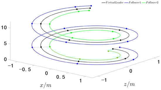
Figure 1.
Actual trajectory tracking curves for the AUVs.
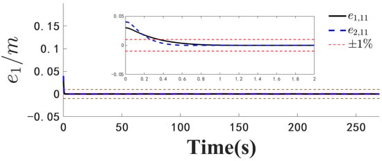
Figure 2.
Position error .
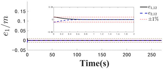
Figure 3.
Position error .
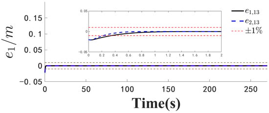
Figure 4.
Position error .
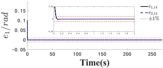
Figure 5.
Position error .
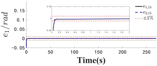
Figure 6.
Position error .
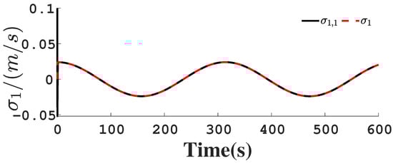
Figure 7.
Follower’s velocity .
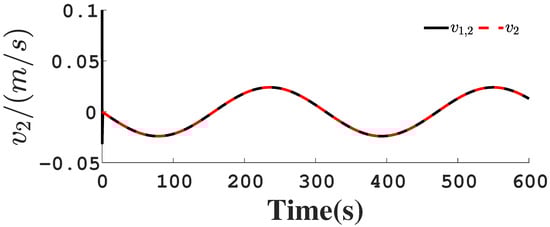
Figure 8.
Follower’s velocity .
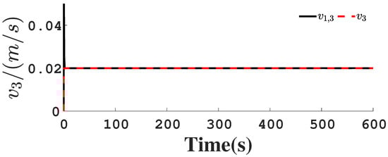
Figure 9.
Follower’s velocity .
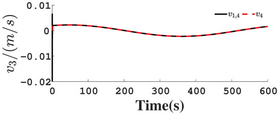
Figure 10.
Follower’s velocity .
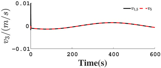
Figure 11.
Follower’s velocity .
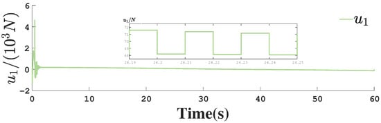
Figure 12.
Control input for actuator 1.
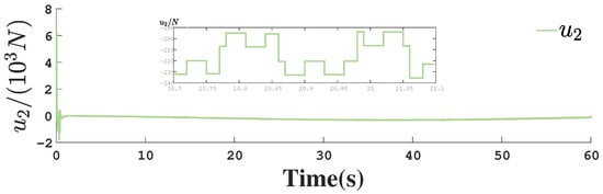
Figure 13.
Control input for actuator 2.
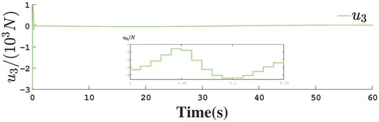
Figure 14.
Control input for actuator 3.
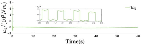
Figure 15.
Control input for actuator 4.
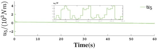
Figure 16.
Control input for actuator 5.
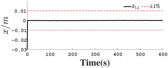
Figure 17.
Position observation error .
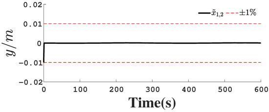
Figure 18.
Position observation error .
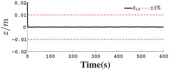
Figure 19.
Position observation error .
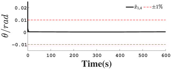
Figure 20.
Position observation error .
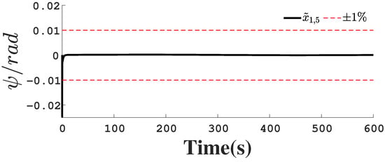
Figure 21.
Position observation error .
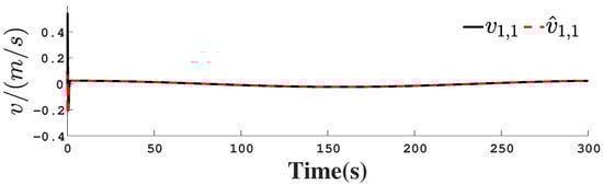
Figure 22.
Unmeasurable velocity observation curve.
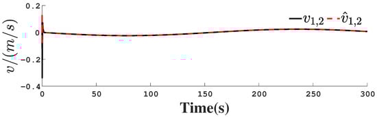
Figure 23.
Unmeasurable velocity observation curve.
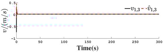
Figure 24.
Unmeasurable velocity observation curve.
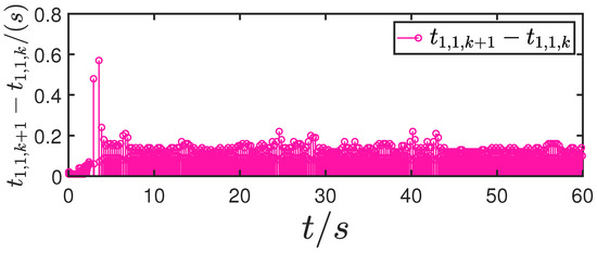
Figure 25.
Update interval for actuator 1.
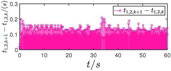
Figure 26.
Update interval for actuator 2.
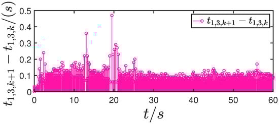
Figure 27.
Update interval for actuator 3.
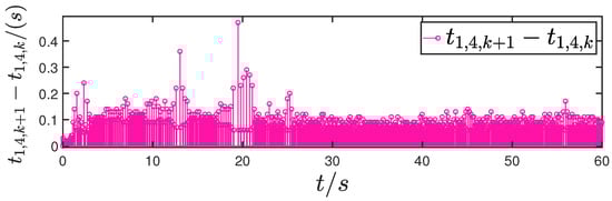
Figure 28.
Update interval for actuator 4.
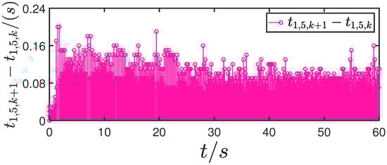
Figure 29.
Update interval for actuator 5.
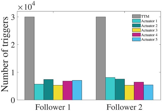
Figure 30.
Control signal update interval for the follower AUVs.
Figure 1, Figure 2, Figure 3, Figure 4, Figure 5, Figure 6, Figure 7, Figure 8, Figure 9, Figure 10, Figure 11, Figure 12, Figure 13, Figure 14, Figure 15, Figure 16, Figure 17, Figure 18, Figure 19, Figure 20, Figure 21, Figure 22, Figure 23, Figure 24, Figure 25, Figure 26, Figure 27, Figure 28 and Figure 29 confirm the boundedness of all system signals. Specifically, Figure 1 demonstrates close convergence between the AUV’s actual trajectory and the reference path, validating the tracking performance of the proposed controller. Figure 2, Figure 3, Figure 4, Figure 5 and Figure 6 further reveal that the state 1 tracking error remains confined within a 1% error margin, while Figure 7, Figure 8, Figure 9, Figure 10 and Figure 11 corroborate effective velocity tracking. The actuator inputs, depicted in Figure 12, Figure 13, Figure 14, Figure 15 and Figure 16, exhibit smooth and physically realizable profiles upon system stabilization. The observer’s efficacy is evidenced in Figure 17, Figure 18, Figure 19, Figure 20, Figure 21, Figure 22, Figure 23 and Figure 24. Figure 17, Figure 18, Figure 19, Figure 20 and Figure 21 show rapid convergence of position/attitude estimation errors to a near-zero residual band, whereas Figure 22, Figure 23 and Figure 24 confirm the accurate reconstruction of unmeasurable linear and angular velocities. The event-triggering mechanism (ETM) performance is quantified in Figure 30 and Table 1. Compared to time-triggered schemes (TTM), the ETM reduces trigger instances by 75–82% across actuators (e.g., 5701 triggers for Actuator 1 versus TTM’s fixed-interval triggering), significantly alleviating computational and communication loads. Crucially, Figure 25, Figure 26, Figure 27, Figure 28 and Figure 29 verify the absence of Zeno behavior. These results collectively substantiate the control scheme’s effectiveness in achieving precise tracking, robust observation, and resource-efficient implementation.

Table 1.
Table of event triggers for each AUV.
In order to demonstrate the superiority of the present method (RSDASO), it was compared with the Fixed Time Disturbance Observer (FTDO) [31] and Finite Time Disturbance Observer (FDO). The simulation results are shown in Figure 31, Figure 32 and Figure 33. The figures demonstrate a comparison of the AUV position and attitude tracking errors under different control strategies. As shown in Figure 31, the proposed RSDASO method (black curve) exhibited significant advantages over the two control strategies, FTDO (blue dashed line) and FDO (red dashed line), in terms of the position tracking error . During the initial stage (near ), although the errors of all three methods showed notable changes, the RSDASO method demonstrated a faster error convergence rate, rapidly approaching zero error. From to 1 s, its error fluctuated with a smaller amplitude and stabilized quickly. After the system stabilized, the error curve of the RSDASO method remained within a narrow fluctuation range, maintaining a level close to zero, which highlights its high positional tracking stability. In contrast, while the error curves of FTDO and FDO also tended toward zero, their fluctuation amplitudes were larger than those of the RSDASO method, particularly for the FDO method (red dashed line), which exhibited more pronounced error fluctuations throughout the entire time period. Further analysis of the position tracking errors in the other two degrees of freedom, as shown in Figure 32 and Figure 33, revealed that the RSDASO method achieved faster error convergence in the initial stage, exhibited smoother error curves with significantly smaller fluctuation amplitudes during the intermediate stage, and stabilized errors at a level closer to zero with the smallest fluctuation range in the later stage. Collectively, the RSDASO method demonstrated superior performance in convergence speed, stability, and error control accuracy across all degrees of freedom, underscoring its excellent efficacy in trajectory tracking control.
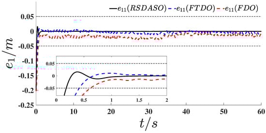
Figure 31.
Comparison of position tracking errors in simulation.
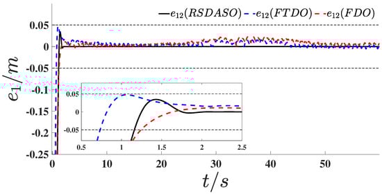
Figure 32.
Comparison of position tracking errors in simulation.
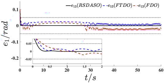
Figure 33.
Comparison of position tracking errors in simulation.
5. Conclusions
This study effectively addressed the challenging issues associated with multi-AUV formation systems, including full-state constraints, unmeasurable states, model uncertainties, limited communication resources, and unknown time-varying external disturbances. It presented a fixed-time accurate formation control method for multi-AUVs based on a switching threshold event-triggering mechanism. The theoretical demonstration showed that (1) all system errors (including observer estimation errors) converged within a fixed time interval and (2) the communication burden was significantly reduced while rigorously avoiding Zeno behavior. The efficacy of the proposed control strategy was conclusively validated through comprehensive simulation examples. Future work will focus on addressing time-delay issues in multi-AUV formation control systems, which represent a critical challenge in practical underwater applications.
Author Contributions
Conceptualization, H.W.; Formal analysis, Y.C., Methodology, H.W.; Project administration, Y.C.; Validation, H.W. and Y.C.; Visualization, H.W. and X.W.; Writing—original draft, H.W. All authors have read and agreed to the published version of the manuscript.
Funding
This work was supported by special projects in the key fields of colleges and universities in Guangdong Province, China (no. 2022ZDZX1070), the characteristic innovation projects of colleges and universities in Guangdong Province, China (no. 2022KTSCX299), and the research project of Guangzhou City Polytechnic. (no. KYTD2023004).
Data Availability Statement
All relevant data are within the paper.
Conflicts of Interest
The authors declare no competing interests.
Appendix A
The pseudocode representation of the proposed control algorithm simulation experiment is shown in the following Algorithm A1.
| Algorithm A1 Event-Triggered Control for AUV | ||
| Require: Step size , total time T, AUV parameters | ||
| Ensure: Position and orientation of the AUV | ||
| 1: | Initialize | ▷ Initial control input |
| 2: | for to T by do | |
| 3: | Calculate_Observer_State(t) | ▷ State estimation |
| 4: | Calculate_Virtual_Control_Law(t) | ▷ Nominal control |
| 5: | Calculate__ETM(t) | ▷ Event-triggered mechanism |
| 6: | if then | ▷ Triggering condition 1 |
| 7: | if then | |
| 8: | ▷ Update control | |
| 9: | else | |
| 10: | ▷ Hold previous value | |
| 11: | end if | |
| 12: | else | ▷ Triggering condition 2 |
| 13: | if then | |
| 14: | ||
| 15: | else | |
| 16: | ||
| 17: | end if | |
| 18: | end if | |
| 19: | Calculate__Actuator | ▷ Apply control |
| 20: | end for | |
Appendix B
The parameters of the AUV dynamic model that were utilized in the simulation experiments are shown in Table A1.
Table A1.
AUV physical model parameters.
Table A1.
AUV physical model parameters.
| Element | Value | Element | Value | Element | Value |
|---|---|---|---|---|---|
| m | 390 | 305.67 | 305.67 | ||
| −49.12 | −311.52 | −311.52 | |||
| −20 | −200 | −200 | |||
| −30 | −300 | −300 | |||
| −100 | −87.63 | 300 | |||
| −200 | −87.63 | −300 |
Appendix C
For the proposed switching threshold event-triggering mechanism, we can analyze the following two cases.
For the time interval , where the time-varying parameters satisfy and , the following relationship can be derived:
From Lemma 3 and Young’s inequality, the critical bounding relationship emerges:
Case 2: . Similarly, for ∀ t ∈, one can obtain that , with . Thus, it can be obtained that
Combining Cases 1–2 yields
References
- He, S.; Kou, L.; Li, Y.; Xiang, J. Robust Orientation-Sensitive Trajectory Tracking of Underactuated Autonomous Underwater Vehicles. IEEE Trans. Ind. Electron. 2021, 68, 8464–8473. [Google Scholar] [CrossRef]
- Braginsky, B.; Baruch, A.; Guterman, H. Development of an Autonomous Surface Vehicle capable of tracking Autonomous Underwater Vehicles. Ocean Eng. 2020, 197, 106868. [Google Scholar] [CrossRef]
- Yang, T.; Yu, S.; Yan, Y. Formation control of multiple underwater vehicles subject to communication faults and uncertainties. Appl. Ocean Res. 2019, 82, 109–116. [Google Scholar] [CrossRef]
- Gao, Z.; Guo, G. Fixed-time sliding mode formation control of AUVs based on a disturbance observer. IEEE/CAA J. Autom. Sin. 2020, 7, 539–545. [Google Scholar] [CrossRef]
- Gu, N.; Wang, D.; Peng, Z.; Liu, L. Observer-Based Finite-Time Control for Distributed Path Maneuvering of Underactuated Unmanned Surface Vehicles With Collision Avoidance and Connectivity Preservation. IEEE Trans. Syst. Man. Cybern. Syst. 2021, 51, 5105–5115. [Google Scholar] [CrossRef]
- Liu, M.; Liu, K.; Zhu, P.; Zhang, G.; Ma, X.; Shang, M. Data-Driven Remote Center of Cyclic Motion (RC2M) Control for Redundant Robots with Rod-Shaped End-Effector. IEEE Trans. Ind. Informatics 2024, 20, 6772–6780. [Google Scholar] [CrossRef]
- Yang, T.; Yi, X.; Wu, J.; Yuan, Y.; Wu, D.; Meng, Z.; Hong, Y.; Wang, H.; Lin, Z.; Johansson, K.H. A survey of distributed optimization. Annu. Rev. Control 2019, 47, 278–305. [Google Scholar] [CrossRef]
- Wang, H.; Su, B. Event-triggered formation control of AUVs with fixed-time RBF disturbance observer. Appl. Ocean Res. 2021, 112, 102638. [Google Scholar] [CrossRef]
- Zong, G.; Yang, D.; Lam, J.; Song, X. Fault-Tolerant Control of Switched LPV Systems: A Bumpless Transfer Approach. IEEE/ASME Trans. Mechatronics 2022, 27, 1436–1446. [Google Scholar]
- Yang, D.; Zong, G.; Shi, Y.; Shi, P. Adaptive Tracking Control of Hybrid Switching Markovian Systems with Its Applications. SIAM J. Control Optim. 2023, 61, 434–457. [Google Scholar] [CrossRef]
- Kumar, N.; Rani, M. An efficient hybrid approach for trajectory tracking control of autonomous underwater vehicles. Appl. Ocean Res. 2020, 95, 102053. [Google Scholar] [CrossRef]
- Elhaki, O.; Shojaei, K. Neural network-based target tracking control of underactuated autonomous underwater vehicles with a prescribed performance. Ocean Eng. 2018, 167, 239–256. [Google Scholar] [CrossRef]
- Chen, G.; Dong, J. Approximate Optimal Adaptive Prescribed Performance Fault-Tolerant Control for Autonomous Underwater Vehicle Based on Self-Organizing Neural Networks. IEEE Trans. Veh. Technol. 2024, 73, 9776–9785. [Google Scholar] [CrossRef]
- Li, J.; Du, J.; Chang, W.J. Robust time-varying formation control for underactuated autonomous underwater vehicles with disturbances under input saturation. Ocean Eng. 2019, 179, 180–188. [Google Scholar] [CrossRef]
- Wang, N.; Sun, Z.; Yin, J.; Zou, Z.; Su, S.F. Fuzzy unknown observer-based robust adaptive path following control of underactuated surface vehicles subject to multiple unknowns. Ocean Eng. 2019, 176, 57–64. [Google Scholar] [CrossRef]
- Li, T.; Zhao, R.; Chen, C.L.P.; Fang, L.; Liu, C. Finite-Time Formation Control of Under-Actuated Ships Using Nonlinear Sliding Mode Control. IEEE Trans. Cybern. 2018, 48, 3243–3253. [Google Scholar] [CrossRef]
- Zhang, L.; Qi, W.; Kao, Y.; Gao, X.; Zhao, L. New results on finite-time stabilization for stochastic systems with time-varying delay. Int. J. Control Autom. Syst. 2018, 16, 649–658. [Google Scholar] [CrossRef]
- Zhang, H.; Li, B.; Xiao, B.; Yang, Y.; Ling, J. Nonsingular recursive-structure sliding mode control for high-order nonlinear systems and an application in a wheeled mobile robot. ISA Trans. 2022, 130, 553–564. [Google Scholar] [CrossRef]
- Polyakov, A. Nonlinear Feedback Design for Fixed-Time Stabilization of Linear Control Systems. IEEE Trans. Autom. Control 2012, 57, 2106–2110. [Google Scholar] [CrossRef]
- Wan, L.; Cao, Y.; Sun, Y.; Qin, H. Fault-tolerant trajectory tracking control for unmanned surface vehicle with actuator faults based on a fast fixed-time system. ISA Trans. 2022, 130, 79–91. [Google Scholar] [CrossRef]
- Sahu, B.K.; Subudhi, B. Flocking Control of Multiple AUVs Based on Fuzzy Potential Functions. IEEE Trans. Fuzzy Syst. 2018, 26, 2539–2551. [Google Scholar] [CrossRef]
- Shojaei, K. Neural network formation control of underactuated autonomous underwater vehicles with saturating actuators. Neurocomputing 2016, 194, 372–384. [Google Scholar] [CrossRef]
- Qu, X.; Liang, X.; Hou, Y. Fuzzy state observer-based cooperative path-following control of autonomous underwater vehicles with unknown dynamics and ocean disturbances. Int. J. Fuzzy Syst. 2021, 23, 1849–1859. [Google Scholar] [CrossRef]
- Wang, A.; Liu, L.; Qiu, J.; Feng, G. Event-Triggered Robust Adaptive Fuzzy Control for a Class of Nonlinear Systems. IEEE Trans. Fuzzy Syst. 2019, 27, 1648–1658. [Google Scholar] [CrossRef]
- Deng, Y.; Zhang, X.; Im, N.; Zhang, G.; Zhang, Q. Event-triggered robust fuzzy path following control for underactuated ships with input saturation. Ocean Eng. 2019, 186, 106122. [Google Scholar] [CrossRef]
- Ba, D.; Li, Y.X.; Tong, S. Fixed-time adaptive neural tracking control for a class of uncertain nonstrict nonlinear systems. Neurocomputing 2019, 363, 273–280. [Google Scholar] [CrossRef]
- Jin, X. Adaptive fixed-time control for MIMO nonlinear systems with asymmetric output constraints using universal barrier functions. IEEE Trans. Autom. Control 2019, 64, 3046–3053. [Google Scholar] [CrossRef]
- Zhang, J.; Li, S.; Xiang, Z. Adaptive fuzzy output feedback event-triggered control for a class of switched nonlinear systems with sensor failures. IEEE Trans. Circuits Syst. I Regul. Pap. 2020, 67, 5336–5346. [Google Scholar] [CrossRef]
- Liu, Y.; Ma, H. Adaptive fuzzy tracking control of nonlinear switched stochastic systems with prescribed performance and unknown control directions. IEEE Trans. Syst. Man Cybern. Syst. 2020, 50, 590–599. [Google Scholar] [CrossRef]
- Liu, Y.J.; Lu, S.; Tong, S. Neural network controller design for an uncertain robot with time-varying output constraint. IEEE Trans. Syst. Man Cybern. Syst. 2017, 47, 2060–2068. [Google Scholar] [CrossRef]
- Liu, S.; Liu, Y.; Wang, N. Nonlinear disturbance observer-based backstepping finite-time sliding mode tracking control of underwater vehicles with system uncertainties and external disturbances. Nonlinear Dyn. 2017, 88, 465–476. [Google Scholar] [CrossRef]
- Wang, N.; Lv, S.; Er, M.J.; Chen, W.H. Fast and accurate trajectory tracking control of an autonomous surface vehicle with unmodeled dynamics and disturbances. IEEE Trans. Intell. Veh. 2016, 1, 230–243. [Google Scholar] [CrossRef]
- Xing, L.; Wen, C.; Liu, Z.; Su, H.; Cai, J. Event-triggered adaptive control for a class of uncertain nonlinear systems. IEEE Trans. Autom. Control 2017, 62, 2071–2076. [Google Scholar] [CrossRef]
- Zhang, J.; Yu, S.; Yan, Y. Fixed-time output feedback trajectory tracking control of marine surface vessels subject to unknown external disturbances and uncertainties. ISA Trans. 2019, 93, 145–155. [Google Scholar] [CrossRef] [PubMed]
- Zhao, X.; Wang, X.; Ma, L.; Zong, G. Fuzzy approximation based asymptotic tracking control for a class of uncertain switched nonlinear systems. IEEE Trans. Fuzzy Syst. 2020, 28, 632–644. [Google Scholar] [CrossRef]
- Basin, M.; Yu, P.; Shtessel, Y. Finite- and fixed-time differentiators utilising HOSM techniques. IET Control Theory Appl. 2017, 11, 1144–1152. [Google Scholar] [CrossRef]
Disclaimer/Publisher’s Note: The statements, opinions and data contained in all publications are solely those of the individual author(s) and contributor(s) and not of MDPI and/or the editor(s). MDPI and/or the editor(s) disclaim responsibility for any injury to people or property resulting from any ideas, methods, instructions or products referred to in the content. |
© 2025 by the authors. Licensee MDPI, Basel, Switzerland. This article is an open access article distributed under the terms and conditions of the Creative Commons Attribution (CC BY) license (https://creativecommons.org/licenses/by/4.0/).