Linearly Coupled Quantum Harmonic Oscillators and Their Quantum Entanglement

Abstract

In many applications of quantum optics, nonlinear physics, molecular chemistry and biophysics, one can encounter models in which the coupled quantum harmonic oscillator provides an explanation for many physical phenomena and effects. In general, these are harmonic oscillators coupled via coordinates and momenta, which can be represented as $\widehat{H}={\sum }_{i=1}^2\left({\displaystyle \frac{{\widehat{p}}_i^2}{2m_i}}+{\displaystyle \frac{m_i{\omega }_i^2}{2}}{x}_i^2\right)+{\widehat{H}}_{int}$, where the interaction of two oscillators ${\widehat{H}}_{int}=i{k}_1{x}_1{\widehat{p}}_2+i{k}_2{x}_2{\widehat{p}}_1+k_3{x}_1{x}_2-k_4{\widehat{p}}_1{\widehat{p}}_2$. Despite the importance of this system, there is currently no general solution to the Schrödinger equation that takes into account arbitrary initial states of the oscillators. Here, this problem is solved in analytical form, and it is shown that the probability of finding the system in any states and quantum entanglement depends only on one coefficient $R\in (0,1)$ for the initial factorizable Fock states of the oscillator and depends on two parameters $R\in (0,1)$ and $\varphi$ for arbitrary initial states. These two parameters $R\in (0,1)$ and $\varphi$ include the entire set of variables of the system under consideration.

1. Introduction

The study of harmonic oscillators, the connection between which is realized through coordinates and momenta, is a current direction in modern physics. Interest in this area is driven by a wide range of applications where models of such systems find application: from quantum optics [1,2,3] and nonlinear physics [4,5,6,7,8,9,10,11,12,13] to molecular chemistry [14,15,16] and biophysics [17,18,19]. Physical models of coupled harmonic oscillators have been successfully used in various studies, including the Lee model in quantum field theory [5,6,7]. A similar Hamiltonian is used in biophysics to explain the processes occurring during photosynthesis [17,18,19,20]. It has long been known that in quantum optics, such phenomena as frequency conversion, parametric amplification, and Raman and Brillouin scattering can be described using the coupled harmonic oscillator model [21,22,23]. In modern studies of coupled quantum harmonic oscillators, the main emphasis is on their quantum entanglement, which forms a separate direction for research in quantum physics. Quantum communication protocols, in particular quantum cryptography [24], quantum dense coding [25], quantum computational algorithms [26], and quantum-state teleportation [27,28], can be interpreted using entangled states. This is due to the fact that such oscillators adequately model real physical systems, such as thermal vibrations of coupled atoms, photons in resonators, optomechanical cooling, ions in ion traps, linear beam splitters and others [3,29,30,31,32,33,34]. Moreover, coupled harmonic oscillators are one of the key models for studying quantum decoherence (see, e.g., [13,35]).

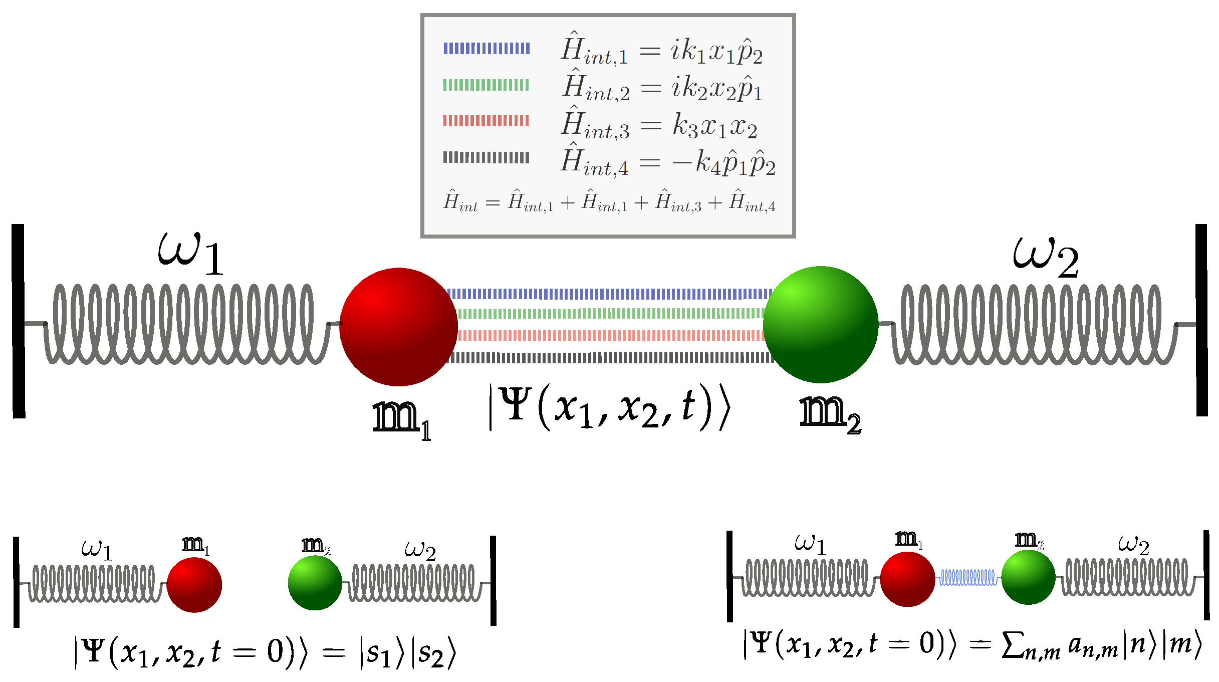
Thus, many systems can be represented as quantum harmonic oscillators coupled in coordinates and momenta with a Hamiltonian in the form

$$\begin{array}{c}\hfill \widehat{H}=\sum _{i=1}^2\left({\displaystyle \frac{{\widehat{p}}_i^2}{2m_i}}+{\displaystyle \frac{m_i{\omega }_i^2}{2}}{x}_i^2\right)+{\widehat{H}}_{int},\\ \hfill {\widehat{H}}_{int}=i{k}_1{x}_1{\widehat{p}}_2+i{k}_2{x}_2{\widehat{p}}_1+k_3{x}_1{x}_2-k_4{\widehat{p}}_1{\widehat{p}}_2,\end{array}$$

(1)

where ${\widehat{p}}_k=-i\hslash {\displaystyle \frac{\partial }{\partial x_k}}$ ($k=1,2$) is the momentum operator; $m_i,{\omega }_i$ are the mass and frequency of oscillator i, respectively; coefficients $k_1,k_2,k_3,k_4$ determine the coupled between two oscillators with the interaction energy ${\widehat{H}}_{int}$. Often, in quantum optics, Equation (1) can be seen through the operators of particle creation ${\widehat{a}}_i$ and annihilation ${\widehat{a}}_i^{†}$; in this case, the Hamiltonian will be

$$\begin{array}{c}\hfill \widehat{H}=\sum _{i=1}^2\hslash {\omega }_i{\widehat{a}}_i^{†}{\widehat{a}}_i+{\widehat{H}}_{int},\\ \hfill {\widehat{H}}_{int}={\alpha }_{mm}{\widehat{a}}_1{\widehat{a}}_2+{\alpha }_{mp}{\widehat{a}}_1{\widehat{a}}_2^{†}+{\alpha }_{pm}{\widehat{a}}_1^{†}{\widehat{a}}_2+{\alpha }_{pp}{\widehat{a}}_1^{†}{\widehat{a}}_2^{†},\end{array}$$

(2)

where ${\alpha }_{mm},{\alpha }_{mp},{\alpha }_{pm},{\alpha }_{pp}$ are some constants (below, we will show the connection between these constants and the constants in Equation (1)).

The solution of the Schrödinger equation $\widehat{H}\Psi =i\hslash {\displaystyle \frac{\partial \Psi }{\partial t}}$ in general form is currently unknown, taking into account arbitrary initial states, which can be factorized and can be in the Fock state $|s_1\rangle |s_2\rangle$ or non-factorizable, i.e., being in a superposition ${\sum }_{n,m}{a}_{n,m}|n\rangle |m\rangle$; see Figure 1. There are only some special cases of this solution, where the quantum entanglement of such oscillators is also studied. For example, in the works [9,33,36,37], the solution and quantum entanglement of such a system were obtained for $k_1=k_2=k_4=0$, and in the work [38], a solution was found for $k_2=k_3=k_4=0$. In the works [39,40,41], the solution for $k_1=k_2=0$ was studied. Various special cases can be found in the works [1,2,3] (see also the references of these works).

It is well known that to study the quantum entanglement of a two-component system, it is necessary not only to find a solution $|\Psi (x_1,x_2,t)\rangle$ of the Schrödinger equation with the Hamiltonian (1), but also to find the decomposition of this solution into Schmidt modes. By the Schmidt theorem [42,43], the wave function $|\Psi (x_1,x_2,t)\rangle$ of two interacting systems can be expanded as $|\Psi (x_1,x_2,t)\rangle ={\sum }_k\sqrt{{\lambda }_k\left(t\right)}|u_k(x_1,t)\rangle |v_k(x_2,t)\rangle$, where $|u_k(x_1,t)\rangle$ is the pure state of the first system, and $|v_k(x_2,t)\rangle$ is the pure state of the second system, where ${\lambda }_k$ is the Schmidt mode. To calculate entanglement, one can use various measures of it; for example, the Schmidt parameter [42,43] $K={\left({\sum }_k{\lambda }_k^2\right)}^{-1}$ or the von Neumann entropy [37,44] $S_N=-{\sum }_k{\lambda }_{k}ln\left({\lambda }_k\right)$. We also add that in this paper we study quantum entanglement for a dynamic system where the non-stationary Schrödinger equation is solved. This means that at the initial time $t=0$, the system of oscillators was in the initial state $|{\Psi }_{in}\rangle$, but the considered connection arises at $t>0$ in the system as a result of some process (depending on the problem under study), as a result of which the dynamics of the system appear.

As a result, a solution to the non-stationary Schrödinger equation was found in the analytical form $|\Psi (x_1,x_2,t)\rangle$ and it was shown that this solution depends on only two parameters, which include all the quantities of the system under consideration. This solution made it possible to find the Schmidt mode and calculate the quantum entanglement of the system under study depending on the initial conditions. It was shown that quantum entanglement depends only on one coefficient $R\in (0,1)$ for the initial Fock states of the oscillator, and depends on two parameters $R\in (0,1)$ and $\varphi$ for arbitrary initial states. These two parameters $R\in (0,1)$ and $\varphi$ include the entire set of variables of the system under consideration.

2. Solution of the Non-Stationary Schrödinger Equation for Arbitrary Initial States

Let us consider the non-stationary Schrödinger equation $\widehat{H}\Psi =i\hslash {\displaystyle \frac{\partial \Psi }{\partial t}}$ with the Hamiltonian (1). We choose the initial conditions in the general form, i.e., $|\Psi (x_1,x_2,t=0)\rangle ={\sum }_{n,m}{a}_{n,m}|n\rangle |m\rangle$, which defines a superposition of the Fock states (with ${\widehat{H}}_{int}=0$) for the 1st and 2nd oscillators, respectively. For now, we will not define the summation ${\sum }_{n,m}$ (this will be carried out below) and will assume that it can be any. We add that the initial condition can be represented in a different form using the Schmidt expansion, i.e., $|\Psi (x_1,x_2,t=0)\rangle ={\sum }_{n,m}{a}_{n,m}|n\rangle |m\rangle ={\sum }_{n=0}^N{b}_n|{\Phi }_n^A\rangle |{\Phi }_n^B\rangle$, where $|{\Phi }_n^A\rangle$ and $|{\Phi }_n^B\rangle$ are some states for the first (system A) and second (system B) oscillators, and N is the Schmidt rank, which is defined as $N=min(dim\left(H_A\right),dim\left(H_B\right))$. However, the Schmidt decomposition cannot be used directly, since the states $|{\Phi }_n^A\rangle$ and $|{\Phi }_n^B\rangle$ are not defined. For example, the simplest version of the initial conditions is $|\Psi (t=0)\rangle =|s_1\rangle |s_2\rangle$, where $s_1$ and $s_2$ are the quantum numbers of the first and second oscillators before the interaction, in this case $a_{n,m}=a_{s_1,s_2}=1$, and all other coefficients are zero.

Next, to solve Equation (1) it is convenient to move to dimensionless variables; to achieve this, we need to replace $\sqrt{{\displaystyle \frac{m_i{\omega }_i}{\hslash }}}{x}_i\to x_i$, we get

$$\begin{array}{c}\hfill \widehat{H}={\displaystyle \frac{1}{2}}\sum _{i=1}^2\hslash {\omega }_i\left(-{\displaystyle \frac{{\partial }^2}{\partial x_i^2}}+x_i^2\right)+{\widehat{H}}_{int},\\ \hfill {\widehat{H}}_{int}=A_{12}{x}_1{\displaystyle \frac{\partial }{\partial x_2}}+A_{21}{x}_2{\displaystyle \frac{\partial }{\partial x_1}}+B{x}_1{x}_2+C{\displaystyle \frac{\partial }{\partial x_1}}{\displaystyle \frac{\partial }{\partial x_2}},\\ \hfill A_{12}=\hslash k_1\sqrt{{\displaystyle \frac{m_2{\omega }_2}{m_1{\omega }_1}}},A_{21}=\hslash k_2\sqrt{{\displaystyle \frac{m_1{\omega }_1}{m_2{\omega }_2}}},B={\displaystyle \frac{\hslash k_3}{\sqrt{m_1{\omega }_1{m}_2{\omega }_2}}},C=\hslash k_4\sqrt{m_1{\omega }_1{m}_2{\omega }_2}.\end{array}$$

(3)

If we introduce the well-known annihilation operators ${\widehat{a}}_i={\displaystyle \frac{1}{\sqrt{2}}}(x_i+{\displaystyle \frac{\partial }{\partial x_i}})$ and creation ${\widehat{a}}_i^{†}={\displaystyle \frac{1}{\sqrt{2}}}(x_i-{\displaystyle \frac{\partial }{\partial x_i}})$, then we obtain Equation (2), where

$$\begin{array}{c}\hfill {\alpha }_{mm}={\displaystyle \frac{1}{2}}\left(A_{12}+A_{21}+B+C\right),{\alpha }_{mp}={\displaystyle \frac{1}{2}}\left(-A_{12}+A_{21}+B-C\right),\\ \hfill {\alpha }_{pm}={\displaystyle \frac{1}{2}}\left(A_{12}-A_{21}+B-C\right),{\alpha }_{pp}={\displaystyle \frac{1}{2}}\left(-A_{12}-A_{21}+B+C\right).\end{array}$$

(4)

The solution of differential equations of this type has not been presented in the literature before, except for the recent works [45,46,47], where a method for their solution was proposed. Traditionally, such equations are solved by diagonalizing the Hamiltonian (3) by changing variables, as, for example, in [9,33,36]. In [38], a method was developed to diagonalize the Hamiltonian in the presence of only one of the coefficients $A_{i,j}$ using a unitary transformation, avoiding the change of variables. To solve Equation (3), we combine these two approaches. The first step to diagonalize the Hamiltonian (3) is a change of variables:

$$x_1/\sqrt{\hslash {\omega }_1}=xcos\theta +ysin\theta ,x_2/\sqrt{\hslash {\omega }_2}=\left(-xsin\theta +ycos\theta \right)(1+\delta ),$$

where $\theta$ and $\delta$ are unknown coefficients. Then, in the second step, a unitary transformation is applied to the Hamiltonian depending on the variables $\{x,y\}$ (i.e., $\widehat{H}=\widehat{H}(x,y)$): $\Psi ={\widehat{S}}^{-1}{\Psi }^{\prime }$, where ${\Psi }^{\prime }=\widehat{S}\Psi$. That is, the wave function ${\Psi }^{\prime }$ corresponds to the Hamiltonian ${\widehat{H}}^{\prime }=\widehat{S}\widehat{H}(x,y){\widehat{S}}^{-1}$ under the conditions $\widehat{H}\Psi =E\Psi$ and ${\widehat{H}}^{\prime }{\Psi }^{\prime }=E{\Psi }^{\prime }$, where E is the energy eigenvalue. As a unitary operator $\widehat{S}$, we choose

$$\widehat{S}=e^{i\gamma {\displaystyle \frac{\partial }{\partial x}}{\displaystyle \frac{\partial }{\partial y}}}{e}^{i\alpha xy}.$$

Ref. [38], where $\gamma$ and $\alpha$ are also unknown coefficients. Let us add that the physical meaning of this operator and the unitary transformation is the transition to a new frame of reference. As a result, we obtain the Hamiltonian ${\widehat{H}}^{\prime }$ in analytical form, containing four unknown coefficients: $\theta ,\delta ,\gamma ,\alpha$. From Equation (3), we know four coefficients: $A_{12},A_{21},B,C$. By composing a system of fourth-order equations and equating the coefficients of the non-diagonalizable variables to zero, we can bring the Hamiltonian ${\widehat{H}}^{\prime }$ to a diagonal form.

During diagonalization, it is assumed that the oscillators are weakly coupled, i.e., the coupling energies $\{A_{12},A_{21},B,C\}$ are significantly less than the energies of the oscillators themselves $\hslash {\omega }_i$. This assumption allows, firstly, to obtain an analytical solution; secondly, it corresponds to most physical systems, where if this condition is violated, the coupling becomes nonlinear, and, thirdly (as will be shown below), it ensures the conservation of quantum numbers before and after the interaction, which in the case of photons means the conservation of their total number in the system. Here, we have described a solution strategy for bringing the Hamiltonian Equation (3) to diagonal form; the main solution is presented in Appendix A. As a result, accurate to the phase, which can be ignored, we obtain the solution

$$\begin{array}{c}\hfill |\Psi (x_1,x_2,t)\rangle =\sum _{n,m}\sum _{k=0}^{n+m}{a}_{n,m}{c}_{k,n+m-k}^{n,m}|k\rangle |n+m-k\rangle .\\ \hfill c_{p,l}^{n,m}=\sum _{k=0}^{n+m}{A}_{k,n+m-k}^{n,m}{A}_{k,n+m-k}^{*p,l}{e}^{-2ikarccos\left(\sqrt{1-R}sin\varphi \right)},\\ \hfill A_{k,p}^{n,m}={\displaystyle \frac{{\mu }^{k+n}\sqrt{k!p!}}{{(1+{\mu }^2)}^{\frac{s_1+s_2}{2}}\sqrt{n!m!}}}{P}_k^{(-(1+s_1+s_2),p-n)}\left(-{\displaystyle \frac{2+{\mu }^2}{{\mu }^2}}\right),\\ \hfill \mu =\sqrt{1+{\displaystyle \frac{1-R}{R}}{cos}^2\varphi }-cos\varphi \sqrt{{\displaystyle \frac{1-R}{R}}},\end{array}$$

(5)

where $P_{\gamma }^{a,b}\left(x\right)$ are Jacobi polynomials and the condition $n+m=k+p$ is satisfied, i.e., the total number of quantum numbers in the system is conserved. States $|k\rangle =C_k{e}^{-x_1^2/2}{H}_k\left(x_1\right)$ and $|n+m-k\rangle =C_{n+m-k}{e}^{-x_2^2/2}{H}_{n+m-k}\left(x_2\right)$ ($H_n\left(x\right)$ are Hermite polynomials, $C_n$ are known normalization coefficients for a linear oscillator) are states of oscillators in a state without interaction. The coefficients R and $\varphi$ in Equation (5) are defined

$$\begin{array}{c}\hfill R={\displaystyle \frac{{sin}^2\left(\Omega t/2\sqrt{1+{ϵ}^2}\right)}{(1+{ϵ}^2)}},cos\varphi =-ϵ\sqrt{{\displaystyle \frac{R}{1-R}}},\\ \hfill \Omega ={\displaystyle \frac{1}{\hslash }}\sqrt{{|B-C|}^2+{|A_{12}-A_{21}|}^2},ϵ={\displaystyle \frac{{\omega }_2-{\omega }_1}{\Omega }}.\end{array}$$

(6)

In general, Equation (5) does not decompose into Schmidt modes, since the initial state of the oscillators is correlated. It can be seen that if we choose the initial states in the form $|\Psi (x_1,x_2,t=0)\rangle ={\sum }_{n,m}{a}_{n,m}|n\rangle |m\rangle$, where $n+m=N$, i.e., where the total number of quantum numbers is conserved, then Equation (5) can be easily decomposed into Schmidt modes in the form

$$\begin{array}{c}\hfill |\Psi (x_1,x_2,t)\rangle =\sum _{k=0}^N\left(\sum _{n=0}^N{a}_n{c}_{k,N-k}^{n,N-n}\right)|k\rangle |N-k\rangle ,\end{array}$$

(7)

where ${\lambda }_k={\left|{\sum }_{n=0}^N{a}_n{c}_{k,N-k}^{n,N-n}\right|}^2$ is the Schmidt mode ($a_n=a_{n,N-n}$). Let us add that the expansion of the initial state in the form $|\Psi (x_1,x_2,t=0)\rangle ={\sum }_{n=0}^N{a}_n|n\rangle |N-n\rangle$ is the most correct from a physical point of view. Indeed, if our system is isolated and the initial state $|\Psi (x_1,x_2,t=0)\rangle$ was formed as a result of the evolution of this system from a state without connections at all previous moments of time, i.e., $|\Psi (x_1,x_2,t=0)\rangle =e^{-i{\widehat{H}}_0\tau }{\widehat{S}}_e|s_1\rangle |s_2\rangle$, where ${\widehat{S}}_e$ is the evolution operator (defined in the Appendix A), and the operator $e^{-i{\widehat{H}}_0\tau }$ (where ${\widehat{H}}_0=\widehat{H}$ for ${\widehat{H}}_{int}=0$) specifies the evolution of the system after the rupture of connections after the evolution of ${\widehat{S}}_e$. As a result, we can obtain

$$\begin{array}{c}\hfill |\Psi (x_1,x_2,t=0)\rangle =e^{-i{\widehat{H}}_0\tau }{\widehat{S}}_e|s_1\rangle |s_2\rangle =e^{i\phi }\sum _{n=0}^{s_1+s_2}{e}^{in({\omega }_2-{\omega }_1)\tau }{c}_{n,s_1+s_2-n}^{s_1,s_2}|n\rangle |s_1+s_2-n\rangle ,\end{array}$$

where $\phi$ is a inessential phase that does not affect the probabilities. As a result, the coefficient $a_n$ in the Equation (7) will be $a_n=e^{in({\omega }_2-{\omega }_1)\tau }{c}_{n,s_1+s_2-n}^{s_1,s_2}$. So ${\lambda }_k={\left|{\sum }_{n=0}^N{a}_n{c}_{k,N-k}^{n,N-n}\right|}^2$ determines the probability of detecting the system in the states $|k\rangle$ and $|N-k\rangle$. Thus, ${\lambda }_k={\left|{\sum }_{n=0}^N{a}_n{c}_{k,N-k}^{n,N-n}\right|}^2$ determines the probability of detecting the system in states $|k\rangle$ and $|N-k\rangle$ and is the Schmidt mode for the initial state of the system in the form $|\Psi (x_1,x_2,t=0)\rangle ={\sum }_{n=0}^N{a}_n|n\rangle |N-n\rangle$. It is evident that the entire dependence in the wave function is reduced to two variables: R and $\varphi$. The properties of the obtained expressions are such that when calculating ${\lambda }_k$ the dependence on $\varphi$ disappears for the initial condition $|\Psi (x_1,x_2,t=0)\rangle =|s_1\rangle |s_2\rangle$ and the entire dependence is reduced to only one parameter R. This case corresponds to the coefficient $a_n={\delta }_{s_1,n}$ (${\delta }_{i,j}$ is the Kronecker delta) for $N=s_1+s_2$. Since quantum entanglement is calculated via the Schmidt mode ${\lambda }_k$, quantum entanglement depends only on R for this initial condition. This remarkable result allows one to analyze probability and quantum entanglement quite simply. In addition, it is clear that $R\in (0,1)$ is a certain parameter characterizing the degree of interaction of two oscillators. The physical meaning of the parameter R depends on what physical system is described by the Equation (1). For example, the case $A_{12}=A_{21}=C=0$ corresponds to the interaction of a two-mode electromagnetic field in a waveguide beam splitter, and the coefficient R is the reflection coefficient [33,36,37]. It is clear that this coefficient R depends on time t, which is easy to understand, since the interaction time of photons in the beam splitter is determined by its thickness, and therefore depends on the interaction time. In the general case, this coefficient R characterizes the interaction of two systems, each of which in a free state is described by the Hamiltonians ${\widehat{H}}_1$ and ${\widehat{H}}_2$, i.e., free oscillators.

The parameter $\Omega$, expressed in terms of the interaction parameters ${\alpha }_{mm},{\alpha }_{mp},{\alpha }_{pm},{\alpha }_{pp}$ (when representing the Hamiltonian in the form of Equation (2)), takes the form $\Omega ={\displaystyle \frac{\sqrt{2}}{\hslash }}\sqrt{|{\alpha }_{mp}{|}^2+{\left|{\alpha }_{pm}\right|}^2}$. Although the parameters ${\alpha }_{mm}$ and ${\alpha }_{pp}$ are missing in this formula, this is not an error. This simplification arises from the assumption that $\{A_{12},A_{21},B,C\}\ll \hslash {\omega }_i$. In this situation, the quantum numbers (and, equivalently, the number of particles) remain unchanged during the interaction, which is a mathematically rigorous result. The conservation of quantum numbers implies that interaction occurs only through combinations of creation and annihilation operators of the form ${\widehat{a}}_1{\widehat{a}}_2^{†}$ or ${\widehat{a}}_1^{†}{\widehat{a}}_2$. This means that the annihilation operator of the first oscillator is compensated by the creation operator of the second oscillator, and vice versa, maintaining the stability of quantum states. It is interesting to note that, given $\{{\alpha }_{mm},{\alpha }_{mp},{\alpha }_{pm},{\alpha }_{pp}\}\ll \hslash {\omega }_i$, the operators corresponding to the coefficients ${\alpha }_{mm}$ and ${\alpha }_{pp}$ (namely, ${\widehat{a}}_1{\widehat{a}}_2$ and ${\widehat{a}}_1^{†}{\widehat{a}}_2^{†}$) are operators of higher orders of smallness compared to the operators ${\widehat{a}}_1{\widehat{a}}_2^{†}$ and ${\widehat{a}}_1^{†}{\widehat{a}}_2$, even if the parameters ${\alpha }_{mm},{\alpha }_{mp},{\alpha }_{pm},{\alpha }_{pp}$ themselves have comparable values.

The presented results are consistent with previously known special cases, such as those in [9,33,36,37], where the case $A_{12}=A_{21}=C=0$ was considered. This corresponds to the quantum entanglement of photons propagating along two modes in a waveguide beam splitter, as well as to the photon statistics at the output ports of both waveguide and other types of beam splitters [33,34]. The case $A_{21}=B=C=0$ studied in [38] describes a different physical situation: the interaction between a single-mode electromagnetic field and an electron in a magnetic field, which is equivalent to placing an electron at Landau levels in an optical resonator. The works [39,40,41] investigated the interesting case $A_{12}=A_{21}=0$, which under certain conditions can model frequency converters, parametric amplifiers, and Raman and Mandelstam–Brillouin scattering processes. Recent studies [45] have shown the possibility of quantum entanglement of photons on free electrons for modeling, for which, within the framework of the considered approach, although small compared to the energy of the oscillators $\hslash {\omega }_i$, non-zero values of the coefficients $A_{12},A_{21},B,C$ are required. Similarly, this model can describe the interaction of photons with a two-mode electromagnetic field and electrons, both free and bound, which is confirmed by the fact that Equation (1) is part of the general Hamiltonian. In addition, one can imagine a model of mechanical nanoharmonic oscillators linearly coupled to each other through various types of interaction. Thus, the considered model covers a wide range of physical phenomena, both already realized and promising for future research. In general, coupled harmonic oscillators are fundamental models used to describe many physical systems, e.g., [1,2,3] (and the references cited therein).

An analysis of Equation (6) shows that for $A_{12}=A_{21}$ and $B=C$ the frequency $\Omega$ vanishes, which in turn leads to the absence of interaction ($R=0$). This result is important because it demonstrates that, despite the presence of coupling, the interaction can be compensated by different terms of ${\widehat{H}}_{int}$. This means that by changing the parameters $A_{12},A_{21},B,C$, one can control the interaction of oscillators, up to its suppression, while maintaining the coupling between them, i.e., the coupling parameters can remain non-zero. Equation (6) also indicates that significant dynamics of the system are observed under the condition ${\omega }_2-{\omega }_1\lesssim \Omega$, i.e., the frequencies ${\omega }_1$ and ${\omega }_2$ should be close enough, given that we are considering the case $\{A_{12},A_{21},B,C\}\ll \hslash {\omega }_i$.

3. Quantum Entanglement of Oscillators

Let us consider quantum entanglement based on two measures, the Schmidt parameter $K={\left({\sum }_{k=0}^N{\lambda }_k^2\right)}^{-1}$ [42,43] and the von Neumann entropy $S_N=-{\sum }_{k=0}^N{\lambda }_{k}ln{\lambda }_k$ [37,44]. To calculate these measures of quantum entanglement, we must directly use Equation (5) with ${\lambda }_k={\left|{\sum }_{n=0}^N{a}_n{c}_{k,N-k}^{n,N-n}\right|}^2$. To calculate quantum entanglement, we must determine the initial conditions of the system under consideration. Let us choose two variants: the first is the most widely used case in quantum optics $a_n={\delta }_{s_1,n}$ (where $N=s_1+s_2$), and the second case is the equiprobable distribution of states $a_n=1/\sqrt{N+1}$. In the first case, as was said earlier, ${\lambda }_k$ does not depend on the phase $\varphi$, but only on the coefficient R, and the second case depends on the phase $\varphi$. Here, we present only some special cases in analytical form for quantum entanglement for the first case $S_N\left(\right|s_1\rangle ,|s_2\rangle )$ and $K\left(\right|s_1\rangle ,|s_2\rangle )$ and the second case for $K(N,\varphi )$. As an example, we present:

❑

For $K(N,\varphi )$ at $N=1$ and $\varphi =0$

$$\begin{array}{c}\hfill K(1,0)={\displaystyle \frac{2}{(1+4(1-R\left)R\right)}},\end{array}$$

(8)

where the maximum quantum entanglement will be ${\left[K(1,0)\right]}_{max}=2$ at $R=0$ and $R=1$.

❑

For $K(N,\varphi )$ at $N=1$ and ${\displaystyle \frac{\pi }{2}}$

$$\begin{array}{c}\hfill K(1,{\displaystyle \frac{\pi }{2}})=2.\end{array}$$

(9)

❑

For $K(N,\varphi )$ at $N=2$ and $\varphi =0$

$$\begin{array}{c}\hfill K(2,0)={\displaystyle \frac{9}{(3+8R(2+R+3(R-2)R^2))}},\end{array}$$

(10)

where the maximum quantum entanglement will be ${\left[K(2,0)\right]}_{max}=3$ at $R=0$ and $R=1$.

❑

For $K(N,\varphi )$ at $N=2$ and ${\displaystyle \frac{\pi }{2}}$

$$\begin{array}{c}\hfill K(2,{\displaystyle \frac{\pi }{2}})={\displaystyle \frac{3}{(1-8{(1-R)}^2{R}^2)}},\end{array}$$

(11)

where the maximum quantum entanglement will be ${\left[K(2,0)\right]}_{max}=3$ at $R=0$ and $R=1$.

❍

For $S_N\left(\right|s_1\rangle ,|s_2\rangle )$ and $K\left(\right|s_1\rangle ,|s_2\rangle )$ at $s_1=1,s_2=1$

$$\begin{array}{c}\hfill S_N\left(\right|1\rangle ,|1\rangle )=-{(1-2R)}^{2}ln{(1-2R)}^2-4R(1-R)ln\left(2R(1-R)\right),\\ \hfill K\left(\right|1\rangle ,|1\rangle )={\displaystyle \frac{1}{1-8R(1-R)(1-3R(1-R\left)\right)}},\end{array}$$

(12)

where the maximum quantum entanglement will be (for $R=1/2(1\pm 1/\sqrt{3})$)

$$\begin{array}{c}\hfill [S_N\left(\right|1\rangle ,|1\rangle {\left)\right]}_{max}=ln3,[K\left(\right|1\rangle ,|1\rangle {\left)\right]}_{max}=3.\end{array}$$

❍

For $S_N\left(\right|s_1\rangle ,|s_2\rangle )$ and $K\left(\right|s_1\rangle ,|s_2\rangle )$ at $s_1=0,s_2=2$ (similarly for $s_1=2$ and $s_2=0$)

$$\begin{array}{c}\hfill S_N\left(\right|0\rangle ,|2\rangle )=2(-1+R)(Rln2+ln(1-R))-2RlnR,\\ \hfill K\left(\right|0\rangle ,|2\rangle )={\displaystyle \frac{1}{1-2R(1-R)(2-3R(1-R\left)\right)}},\end{array}$$

(13)

where the maximum quantum entanglement will be (for $R=1/2$)

$$\begin{array}{c}\hfill [S_N\left(\right|0\rangle ,|2\rangle {\left)\right]}_{max}={\displaystyle \frac{3}{2}}ln2,[K\left(\right|0\rangle ,|2\rangle {\left)\right]}_{max}=8/3.\end{array}$$

❍

For $S_N\left(\right|s_1\rangle ,|s_2\rangle )$ and $K\left(\right|s_1\rangle ,|s_2\rangle )$ at $s_1=2,s_2=2$

$$\begin{array}{c}\hfill S_N\left(\right|2\rangle ,|2\rangle )=12{(1-2R)}^2(-1+R)Rln\left(-6{(1-2R)}^2(-1+R)R\right)-\\ \hfill 12{(-1+R)}^2{R}^{2}ln\left(6{(-1+R)}^2{R}^2\right)-{(1+6(-1+R)R)}^{2}ln\left({(1+6(-1+R)R)}^2\right),\\ \hfill K\left(\right|2\rangle ,|2\rangle )={\displaystyle \frac{1}{1-24R(1-R)\left(1-3R(1-R)\left(4-5R(1-R)(4-7R(1-R\left)\right)\right)\right)}},\end{array}$$

(14)

where the maximum quantum entanglement will be $[S_N\left(\right|2\rangle ,|2\rangle {\left)\right]}_{max}=1.5381$ for $R=1/2(1\pm 0.3675)$ and ${[K\left(\right|2\rangle ,|2\rangle \left)\right]}_{max}=4.4312$ for $R=1/2(1\pm 0.3898)$.

The quantum entanglement of some particular cases can be found in general form, for example, for the initial state $|s_1\rangle ,|0\rangle$. Using the results of [33] for the initial state $|s\rangle ,|0\rangle$, we obtain

$$\begin{array}{c}\hfill K\left(\right|s\rangle ,|0\rangle )={\displaystyle \frac{1}{{{(1-R)}^{2s}}_2{F}_1\left(-s,-s;1;{\left(\frac{R}{1-R}\right)}^2\right)}},\end{array}$$

(15)

where ₂$F_1(a,b;c;x)$ is Gaussian hypergeometric function. Also, analyzing the Equation (15), you can obtain the maximum of this function at $R=1/2$. With this value of $R=1/2$, one can obtain a simpler expression for quantum entanglement

$$\begin{array}{c}\hfill {[K\left(\right|s\rangle ,|0\rangle \left)\right]}_{max}=2^{2s}{\displaystyle \frac{{(s!)}^2}{\left(2s\right)!}}.\end{array}$$

(16)

This can also be found from parameter K in Equation (16) for large values of the quantum number s, where we obtain $K_{max}(s\gg 1)\to \sqrt{\pi s}$. It can be seen that in this case quantum entanglement is unlimited from above.

There is also another important case, when $s_1=s_2=s$ and $R=1/2$. In this case, Holland–Burnett (HB) [48] states are realized. It is well known that this wave function is of great interest in various fields of physics, for example, in quantum metrology [49,50]. In this case, we obtain

$$\begin{array}{c}\hfill K\left(\right|s\rangle ,|s\rangle )={\displaystyle \frac{\pi {(s!)}^2}{\Gamma {{(s+1/2)}^2}_4{F}_3(1/2,1/2,-s,-s;1,1/2-s,1/2-s;1)}},\end{array}$$

(17)

where $\Gamma \left(x\right)$ is the gamma function, and ₄$F_3(x_1,x_2,x_3,x_4;y_1,y_2,y_3;1)$ is the generalized hypergeometric function. It should be added that the Equation (17) has a fairly simple approximation for sufficiently large s; we obtain it in the form $K\approx s^{0.897}$.

Let us add that for the case $a_n=1/\sqrt{N+1}$, the maximum entanglement is realized at $R=0$ and $R=1$. This means that for these values of R, the wave function at any time t is equal to the wave function at the initial time. Since at the initial time the state of the system is maximally close to a chaotic distribution (since the probability of detecting each of the states is equally probable $|a_n{|}^2=1/(N+1)$ ), the entropy of the system will be maximum, and entropy is a measure of entanglement.

Below are the results of calculations for the initial state $a_n={\delta }_{s_1,n}$ (where $N=s_1+s_2$), quantum entanglement for the von Neumann entropy $S_N$ and the Schmidt parameter K depending on the parameter $R\in (0,1)$ and the dimensionless quantity $\Omega t$ for studying the dynamics of the system; see Figure 2 and Figure 3.

The analysis of the presented figures (Figure 2 and Figure 3) and Equations (12)–(17) allows us to conclude the following. An increase in the quantum numbers $s_1$ and $s_2$ leads to an increase in quantum entanglement. For a fixed sum $s_1+s_2$, the entanglement value changes insignificantly, but when analyzing additional figures we can say that the entanglement reaches its maximum possible value at $s_1=s_2$ for certain values of the parameter R. Quantum entanglement exhibits symmetry with respect to the point $R=1/2$, i.e., the entanglement values coincide for $R=1/2+\Delta R$ and $R=1/2-\Delta R$. We add that the symmetry of quantum entanglement with respect to $R=1/2$ can be explained if R is defined as the reflection coefficient. As a result, if we deviate R from $1/2$ by $\Delta R$ in the direction of decrease, i.e., $R=1/2-\Delta R$, then the number of states that will pass from one oscillator to another will be the same as if we deviate R by $\Delta R$ in the direction of increase, i.e., $R=1/2+\Delta R$. In other words, the oscillators exchange energy equally at $R=1/2\pm \Delta R$. The same exchange of states with respect to $R=1/2\pm \Delta R$ yields the same statistics, which defines quantum entanglement. The dependence of entanglement on R is oscillatory in nature, and the number of oscillations increases with an increase in the sum $s_1+s_2$.

In addition, the graphs demonstrate the oscillatory dynamics of quantum entanglement. This is explained by the exchange of energy between two coupled oscillators, which leads to oscillations of various physical characteristics. In the absence of coupling ($A_{1,2}=A_{2,1}=C=0$), this phenomenon is similar to the pendulum effect, which is also applicable in this situation. It is interesting to note that the period of these oscillations is equal to $\pi$ when $ϵ=0$. In the general case, the period depends on the value of $ϵ$. It is important to note that the minimum level of entanglement corresponds to the smallest quantum numbers, i.e., $s_1=s_2=0$ (no entanglement), and the maximum level is determined by the maximum value of the sum $s_1,s_2$.

We also present figures of quantum entanglement for the Schmidt parameter K in the case of initial conditions in the form $a_n=1/\sqrt{N+1}$. The results are presented in Figure 4.

From Figure 4, it is evident that quantum entanglement will always be maximal at $R=0$ and $R=1$ for the reason explained above in the analysis of Equations (8)–(11). Also evident is the tendency for quantum entanglement to decrease at $R\to 1/2$ and $\varphi \to 0$. We add that with increasing quantum number N, the dependence of entanglement on R and $\varphi$ for $a_n=1/\sqrt{N+1}$ will be close to Figure 4.

It should be noted that for $a_n=1/\sqrt{N+1}$, there is a significant dependence of entanglement on the phase, whereas for $a_n={\delta }_{s_1,n}$ (where $N=s_1+s_2$) there is no such dependence. The dependence of the probability ${\lambda }_k$ on the phase and, as a consequence, entanglement for all $a_n$, except $a_n={\delta }_{s_1,n}$, is easily explained due to the superposition of the initial states $|\Psi (x_1,x_2,t=0)\rangle ={\sum }_{n=0}^N{a}_n|n\rangle |N-n\rangle$. Indeed, each term of the superposition is analogous to the sum ${\sum }_n{b}_n{e}^{i\varphi n}$, and when squaring the absolute value, when calculating a physically measurable quantity, the phase is preserved for $n\ge 2$.

4. Conclusions

In this paper, we find a solution for quantum harmonic oscillators, depicted in Equation (5), linearly related via coordinates and momenta and arbitrary initial conditions determined by $|\Psi (x_1,x_2,t=0)\rangle ={\sum }_{n=0}^N{a}_n|n\rangle |N-n\rangle$. This solution has an analytical form and allows us to calculate the probabilities of finding oscillators in different states $P_k={\left|{\sum }_{n=0}^N{a}_n{c}_{k,N-k}^{n,N-n}\right|}^2$. Also, the probability depends on only one system parameter R for $a_n={\delta }_{s_1,n}$, which significantly simplifies the analysis of the obtained expressions, and in the case of arbitrary initial states it depends on two parameters R and $\varphi$. The Schmidt expansion and the Schmidt parameter ${\lambda }_k={\left|{\sum }_{n=0}^N{a}_n{c}_{k,N-k}^{n,N-n}\right|}^2$ are also found, which allows for calculating the quantum entanglement of the system. It is shown that the number of quantum states is preserved before the interaction, during the interaction and after. Some special cases of quantum entanglement are considered, where the result can be presented in a simple analytical form, and conclusions are drawn. It is worth adding that quantum entanglement is obtained without taking into account the environment, i.e., the external environment. In this case, the environment can significantly affect quantum entanglement [51] and this is a separate topic for study, which is beyond the scope of this work. Let us add that practically unlimited quantum entanglement at large quantum numbers in the initial state is limited from a physical point of view by relativistic effects, which are not considered here. This means that at very high entanglement and a very large number of quantum states at the initial moment of time, the oscillators have very high energy, so high that relativistic effects begin to appear.

References

1. Law, C. Effective Hamiltonian for the radiation in a cavity with a moving mirror and a time-varying dielectric medium. Phys. Rev. A 1994, 49, 433. [Google Scholar] [CrossRef] [PubMed]
2. Tang, J.D.; Cai, Q.Z.; Cheng, Z.D.; Xu, N.; Peng, G.Y.; Chen, P.Q.; Wang, D.G.; Xia, Z.W.; Wang, Y.; Song, H.Z.; et al. A perspective on quantum entanglement in optomechanical systems. Phys. Lett. A 2022, 429, 127966. [Google Scholar] [CrossRef]
3. Aspelmeyer, M.; Kippenberg, T.J.; Marquardt, F. Cavity optomechanics. Rev. Mod. Phys. 2014, 86, 1391. [Google Scholar] [CrossRef]
4. Fano, U. Description of States in Quantum Mechanics by Density Matrix and Operator Techniques. Rev. Mod. Phys. 1957, 29, 74–93. [Google Scholar] [CrossRef]
5. Fetter, A.; Walecka, J. Quantum Theory of Many Particle Systems; McGraw-Hill: New York, NY, USA, 1971; p. 615. [Google Scholar]
6. Kim, Y. Observable gauge transformations in the parton picture. Phys. Rev. Lett. 1989, 63, 348. [Google Scholar] [CrossRef]
7. Han, D.; Kim, Y.; Noz, M. Linear canonical transformations of coherent states in Wigner phase space. III. Two-mode states. Phys. Rev. A 1990, 41, 6233. [Google Scholar] [CrossRef]
8. Iachello, F.; Oss, S. Model of n coupled anharmonic oscillators and applications to octahedral molecules. Phys. Rev. Lett. 1991, 66, 2976. [Google Scholar] [CrossRef]
9. Han, D.; Kim, Y.; Noz, M. Illustrative example of Feynman’s rest of the universe. Am. J. Phys. 1999, 67, 61–66. [Google Scholar] [CrossRef]
10. Prauzner-Bechcicki, J.S. Two-mode squeezed vacuum state coupled to the common thermal reservoir. J. Phys. A Math. Theor. 2004, 37, L173. [Google Scholar] [CrossRef]
11. Joshi, C.; Hutter, A.; Zimmer, F.E.; Jonson, M.; Andersson, E.; Öhberg, P. Quantum entanglement of nanocantilevers. Phys. Rev. A 2010, 82, 043801. [Google Scholar] [CrossRef]
12. Paz, J.P.; Roncaglia, A.J. Dynamics of the Entanglement between Two Oscillators in the Same Environment. Phys. Rev. Lett. 2008, 100, 220401. [Google Scholar] [CrossRef] [PubMed]
13. Galve, F.; Pachon, L.; Zueco, D. Bringing entanglement to the high temperature limit. Phys. Rev. Lett. 2010, 105, 180501. [Google Scholar] [CrossRef] [PubMed]
14. Ikeda, S.; Fillaux, F. Incoherent elastic-neutron-scattering study of the vibrational dynamics and spin-related symmetry of protons in the KHCO3 crystal. Phys. Rev. B 1999, 59, 4134–4145. [Google Scholar] [CrossRef]
15. Fillaux, F. Quantum entanglement and nonlocal proton transfer dynamics in dimers of formic acid and analogues. Chem. Phys. Lett. 2005, 408, 302–306. [Google Scholar] [CrossRef]
16. Delor, M.; Archer, S.A.; Keane, T.; Meijer, A.J.H.M.; Sazanovich, I.V.; Greetham, G.M.; Towrie, M.; Weinstein, J.A. Directing the path of light-induced electron transfer at a molecular fork using vibrational excitation. Nat. Chem. 2017, 9, 1099–1104. [Google Scholar] [CrossRef] [PubMed]
17. Romero, E.; Augulis, R.; Novoderezhkin, V.; Ferretti, M.; Thieme, J.; Zigmantas, D.; van Grondelle, R. Quantum coherence in photosynthesis for efficient solar-energy conversion. Nat. Phys. 2014, 10, 676–682. [Google Scholar] [CrossRef]
18. Fuller, F.D.; Pan, J.; Gelzinis, A.; Butkus, V.; Senlik, S.S.; Wilcox, D.E.; Yocum, C.F.; Valkunas, L.; Abramavicius, D.; Ogilvie, J.P. Vibronic coherence in oxygenic photosynthesis. Nat. Chem. 2014, 6, 706–711. [Google Scholar] [CrossRef]
19. Halpin, A.; Johnson, P.; Tempelaar, R.; Murphy, R.S.; Knoester, J.; Jansen, T.; Miller, R.J.D. Two-dimensional spectroscopy of a molecular dimer unveils the effects of vibronic coupling on exciton coherences. Nat. Chem. 2014, 6, 196–201. [Google Scholar] [CrossRef]
20. Calderon, L.F.; Pachon, L.A. Nonadiabatic sunlight harvesting. Phys. Chem. Chem. Phys. 2020, 22, 12678–12687. [Google Scholar] [CrossRef]
21. Mollow, B.R.; Glauber, R.J. Quantum Theory of Parametric Amplification. I. Phys. Rev. 1967, 160, 1076. [Google Scholar] [CrossRef]
22. Louisell, W.H.; Yariv, A.; Siegman, A.E. Quantum Fluctuations and Noise in Parametric Processes. I. Phys. Rev. 1961, 124, 1646. [Google Scholar] [CrossRef]
23. Lu, Y.C. Quantum Theory of Nonlinear Optical Processes with Time-Dependent Pump Amplitude and Phase: Frequency Conversion. Phys. Rev. A 1974, 8, 1053. [Google Scholar] [CrossRef]
24. Ekert, A. Quantum cryptography based on Bell’s theorem. Phys. Rev. Lett. 1991, 67, 661. [Google Scholar] [CrossRef]
25. Bennett, C.H.; Wiesner, S.J. Communication via one- and two-particle operators on Einstein-Podolsky-Rosen states. Phys. Rev. Lett. 1992, 69, 2881. [Google Scholar] [CrossRef] [PubMed]
26. Shor, P. Scheme for reducing decoherence in quantum computer memory. Phys. Rev. A 1995, 52, R2493. [Google Scholar] [CrossRef]
27. Aspect, A.; Roger, P.G.G. Experimental Tests of Realistic Local Theories via Bell’s Theorem. Phys. Rev. Lett. 1981, 47, 460–463. [Google Scholar] [CrossRef]
28. Samuel, L.; Braunstein, H.; Kimble, J. Teleportation of Continuous Quantum Variables. Phys. Rev. Lett. 1998, 80, 869–872. [Google Scholar]
29. Ockeloen-Korppi, C.F.; Damskägg, E.; Pirkkalainen, J.M.; Asjad, M.; Clerk, A.A.; Massel, F.; Woolley, M.J.; Sillanpää, M.A. Stabilized entanglement of massive mechanical oscillators. Nature 2018, 556, 478–482. [Google Scholar] [CrossRef]
30. Makarov, D.N. Optical-mechanical cooling of a charged resonator. Phys. Rev. A 2019, 99, 033850. [Google Scholar] [CrossRef]
31. Makarov, D.N.; Gusarevich, E.S.; Goshev, A.A.; Makarova, K.A.; Kapustin, S.N.; Kharlamova, A.A.; Tsykareva, Y.V. Quantum entanglement and statistics of photons on a beam splitter in the form of coupled waveguides. Sci. Rep. 2021, 11, 10274. [Google Scholar] [CrossRef]
32. Makarov, D.N. Theory for the Beam Splitter in Quantum Optics: Quantum Entanglement of Photons and Their Statistics, HOM Effect. Mathematics 2022, 10, 4794. [Google Scholar] [CrossRef]
33. Makarov, D. Quantum entanglement and reflection coefficient for coupled harmonic oscillators. Phys. Rev. E 2020, 102, 052213. [Google Scholar] [CrossRef] [PubMed]
34. Campos, R.A.; Saleh, B.E.A.; Teich, M.C. Quantum-mechanical lossless beam splitter: SU(2) symmetry and photon statistics. Phys. Rev. A 1989, 40, 1371. [Google Scholar] [CrossRef]
35. Estrada, A.; Pachon, L. Quantum Limit for Driven Linear Non-Markovian Open-Quantum-Systems. New J. Phys. 2015, 17, 033038. [Google Scholar] [CrossRef]
36. Makarov, D.N. Coupled harmonic oscillators and their quantum entanglement. Phys. Rev. E 2018, 97, 042203. [Google Scholar] [CrossRef] [PubMed]
37. Casini, H.; Huerta, M. Entanglement entropy in free quantum field theory. J. Phys. A Math. Theor. 1996, 42, 504007. [Google Scholar] [CrossRef]
38. Makarov, D.N. Quantum entanglement of a harmonic oscillator with an electromagnetic feld. Sci. Rep. 2018, 8, 8204. [Google Scholar] [CrossRef] [PubMed]
39. Dattoli, G.; Torre, A.; Lorenzutta, S.; Maino, G. Coupled harmonic oscillators, generalized harmonic-oscillator eigenstates and coherent states. Il Nuovo C. B 1996, 111, 811–823. [Google Scholar] [CrossRef]
40. Zuniga, J.; Bastida, A.; Requena, A. Quantum solutions of identical linearly coupled harmonic oscillators using oblique coordinates. J. Phys. B At. Mol. Opt. Phys. 2019, 52, 055101. [Google Scholar] [CrossRef]
41. Zuniga, J.; Bastida, A.; Requena, A. Quantum description of linearly coupled harmonic oscillator systems using oblique coordinates. J. Phys. B At. Mol. Opt. Phys. 2020, 53, 025101. [Google Scholar] [CrossRef]
42. Ekert, A.; Knight, P. Entangled quantum systems and the Schmidt decomposition. Am. J. Phys. 1995, 63, 415–423. [Google Scholar] [CrossRef]
43. Grobe, R.; Rzazewski, K.; Eberly, J. Measure of electron-electron correlation in atomic physics. J. Phys. B 1994, 27, L503–L508. [Google Scholar] [CrossRef]
44. Bennett, C.; Bernstein, H.; Popescu, S.; Schumacher, B. Concentrating partial entanglement by local operations. Phys. Rev. A 1996, 53, 2046–2052. [Google Scholar] [CrossRef] [PubMed]
45. Makarov, D. Quantum entanglement of photons on free electrons. Results Phys. 2023, 49, 106515. [Google Scholar] [CrossRef]
46. Makarov, D. General quantum theory of Thomson scattering. Results Phys. 2023, 52, 106790. [Google Scholar] [CrossRef]
47. Makarov, D. Quantum Theory of Scattering of Nonclassical Fields by Free Electrons. Mathematics 2023, 11, 2094. [Google Scholar] [CrossRef]
48. Holland, M.; Burnett, K. Interferometric detection of optical phase shifts at the heisenberg limit. Phys. Rev. Lett. 1993, 71, 1355. [Google Scholar] [CrossRef]
49. Polino, E.; Valeri, M.; Spagnolo, N.; Sciarrino, F. Photonic Quantum Metrology. AVS Quantum Sci. 2020, 2, 024703. [Google Scholar] [CrossRef]
50. Pezze, L.; Smerzi, A.; Oberthaler, M.K.; Schmied, R.; Treutlein, P. Quantum metrology with nonclassical states of atomic ensembles. Rev. Mod. Phys. 2018, 90, 035005. [Google Scholar] [CrossRef]
51. Pachon, L.A.; Triana, J.F.; Zueco, D.; Brumer, P. Influence of non-Markovian dynamics in equilibrium uncertainty-relations. J. Chem. Phys. 2019, 150, 034105. [Google Scholar] [CrossRef]
Figure 1. The model under consideration is presented in the form of spring pendulums (oscillators), linearly connected in four different ways via coordinates and momenta. In the initial states, i.e., at t = 0 , the system can be in the factorizable state | s 1 | s 2 or, in the general case, in the non-factorizable state n , m a n , m | n | m .
Mathematics 13 01452 g001
Figure 2. The dependence of the von Neumann entropy S N in Figures (a,b), as well as the Schmidt parameter in Figures (c,d) as a function of R (for (a,c)) and Ω t (for (b,d)) is presented. In the figures, the dependencies are presented for different initial values of the quantum numbers s 1 , s 2 , so that s 1 = s 2 . For example, for s 1 = 1 and s 2 = 1 , the notation (1,1) is introduced.
Mathematics 13 01452 g002
Figure 3. The dependence of the von Neumann entropy S N in Figures (a,b), and the Schmidt parameter in Figures (c,d) as a function of R (for (a,c)) and Ω t (for (b,d)) is presented. In the figures, the dependences are presented for different initial values of the quantum numbers s 1 , s 2 , so that s 1 + s 2 = 7 . For example, for s 1 = 1 and s 2 = 6 , the notation (1,6) is introduced.
Mathematics 13 01452 g003
Figure 4. The calculation of the Schmidt parameter K as a function of the parameters R and ϕ with the initial conditions a n = 1 / N + 1 for N = 1 is presented in Figure (a), and in Figure (b) for the case N = 2 .
Mathematics 13 01452 g004
Disclaimer/Publisher’s Note: The statements, opinions and data contained in all publications are solely those of the individual author(s) and contributor(s) and not of MDPI and/or the editor(s). MDPI and/or the editor(s) disclaim responsibility for any injury to people or property resulting from any ideas, methods, instructions or products referred to in the content.