Fixed-Time Event-Triggered Control for High-Order Nonlinear Multi-Agent Systems Under Unknown Stochastic Time Delays

Abstract

In this paper, the fixed-time control for high-order nonlinear multi-agent systems under unknown stochastic time delay is investigated via an event-triggered approach. First of all, RBF neural networks are utilized to approximate the system’s uncertain nonlinearities. After that, an event-triggered scheme, which is designed with a relative threshold for more flexible control, is proposed to alleviate the communication burden. In consideration of the unknown stochastic time delay in the inter-communication among high-order nonlinear multi-agent systems, the Lyapunov–Krasovskii functional (LKF) is used to construct the system’s Lyapunov function, specifically targeting the adverse effects caused by time delay. Further, the fixed-time stability theory is employed to ensure that the convergence time remains independent of the initial values. Finally, the proposed control strategy is validated through numerical simulations.

1. Introduction

High-order nonlinear multi-agent systems are generally composed of a set of subsystems with high-order nonlinear dynamics, which exhibit great potential in practical applications such as the platoon driving of intelligent vehicles [1], formation flying of unmanned aircraft [2], cooperative working of electro-hydraulic systems [3], etc. During recent decades, fruitful results have been yielded in the control of high-order nonlinear multi-agent systems [4,5,6]. However, the inherent uncertainty and nonlinearity in these systems significantly enhance the difficulty of the controller design and reduce the control performance [7]. To this end, fuzzy logic functions and neural networks are frequently deployed in the identification of uncertain nonlinear terms in high-order nonlinear multi-agent systems [8,9,10]. In addition, mutual interactions among subsystems further enhance the difficulty in controlling such a system. In [11], a decentralized nearly optimal controller was designed to cope with the weak interactions between subsystems. The adaptive neural controller was designed to address the strong interconnectivity between subsystems in [12]. With the continuous advancement of research, an increasing number of remarkable achievements have emerged in the control of high-order nonlinear multi-agent systems in recent years [13,14].

For high-order nonlinear multi-agent systems to fulfill given tasks, it is necessary for subsystems to exchange information with each other. However, the limited bandwidth of the communication channel restricts the information transmission between subsystems, which may lead to communication congestion and even system performance reduction. At present, a time-triggered scheme is widely deployed in the control of high-order nonlinear multi-agent systems, which not only exhibits satisfactory control performance but also facilitates system analysis [15,16,17]. However, such periodical sampling will inevitably cause information redundancy and increase energy consumption [18]. In view of this, the event-triggered mechanism (ETM) has been proposed to execute sampling and control only at specific moments [19], which is more effective in fulfilling control tasks and has gained considerable attention in recent studies [20]. For example, the ETM was introduced to reduce unnecessary information transmission for high-order nonlinear multi-agent systems in [21]. In event-triggered control, the triggering threshold, to a certain extent, determines the system control performance [22]. In [23,24], a relative threshold ETM was designed to diminish the sensing cost and communication burden of the system. In [25], a novel dynamic event-triggered mechanism was proposed for continuous-time boiler turbine systems to reduce the number of controller updates and save system resources. In [26], the bipartite time-varying output formation tracking problem of heterogeneous linear multi-agent systems with disturbances was investigated based on adaptive dynamic event-triggered control.

On the other hand, the stochastic time delay arising from communication congestion is also a critical concern in the control of high-order nonlinear multi-agent systems [27]. Time delay, which may reduce the control performance and even lead to system instability, has been extensively discussed in the literature [27,28,29,30,31,32,33,34]. At present, the methodology for dealing with time delay can be roughly divided into the frequency-domain and time-domain approaches [28]. The results under the frequency-domain method are accurate [29], but it is quite difficult to implement for unknown stochastic time delays, especially time delays in nonlinear systems. The time-domain method, which is mainly based on the Lyapunov stability theory, can cope with unknown stochastic delay systems and has received considerable attention in recent years. Yin et al. comprehensively used the Lyapunov–Krasovskii functional (LKF), bilateral neural network adaptive control, and finite covering lemma to address the constant time delay problem in nonlinear systems [27,30,31]. Further, an adaptive control strategy was proposed for stochastic constant time delay [32]. Recently, the unknown stochastic time delay in nonlinear systems has become a hot topic. Phat et al. [33] addressed the time-varying delay issue of nonlinear fractional-order systems by means of robust finite-time control. In [34], a finite-time stability strategy was utilized to improve the performance of the nonlinear time delay system.

In practical control systems, convergence time is undeniably an important consideration [35]. Presently, finite-time control is frequently employed to enhance the system’s transient performance [36,37,38,39]. However, the convergence time of finite-time control is influenced by the system’s initial values, which may not satisfy some practical requirements [40]. Fixed-time control, which has a predetermined convergence time [41], is regarded as a potential solution to enhance system’s transient performance. In [42], a novel sliding mode controller was designed to obtain fixed-time convergence for second-order systems. Subsequently, some fixed-time controllers in the sense of the Lyapunov theory were designed [43,44,45], which made fixed-time control broaden its applicability and increased its popularity. In [43], a fixed-time controller was designed by combining multiple Lyapunov methods and stochastic analysis theory. The fixed-time event-triggered controller was investigated to obtain satisfactory control performance in [44]. Utilizing a series of new Lyapunov functions and modified tuning functions, an adaptive fixed-time consensus controller was designed in [45].

Although lots of studies have been devoted to the control of high-order nonlinear multi-agent systems, literature that specifically considers the communication constraints, time delay, and convergence time simultaneously is rarely seen as far as we are concerned. However, these issues are often required at the same time for better control performance in practical applications. Inspired by the above descriptions, this paper designs a fixed-time event-triggered controller for high-order nonlinear multi-agent systems with unknown stochastic time delays. The main contributions are generalized below.

• The relative threshold ETM designed in this paper can save communication resources compared to the traditional time-triggered mechanism [15,16,17] and offers more flexibility and adaptability compared to the fixed threshold ETM [46].
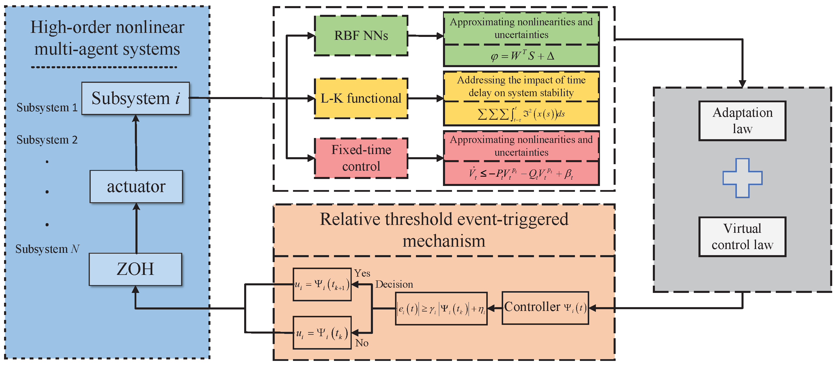
• To tackle prevalent unknown stochastic time delays in high-order nonlinear multi-agent systems, the LKF is introduced to integrate nonlinear time delay functions with the system Lyapunov function. By effectively addressing the time delay functions in the subsequent controller design process, the system exhibits robustness to time delay.
• The designed fixed-time controller ensures that the system can be semiglobal practical fixed-time stable (SPFTS), wherein the convergence time is solely determined by the designed control parameters and is independent of the system’s initial values.

The remainder of this paper is as follows. Section 2 provides preliminary knowledge and problem formulation. Then, the control scheme design and fixed-time stability analysis for high-order nonlinear multi-agent systems are presented in Section 3. Section 4 provides two representative simulation examples to illustrate the theoretical results. Finally, Section 5 concludes this paper.

2. Preliminaries and Problem Formulation

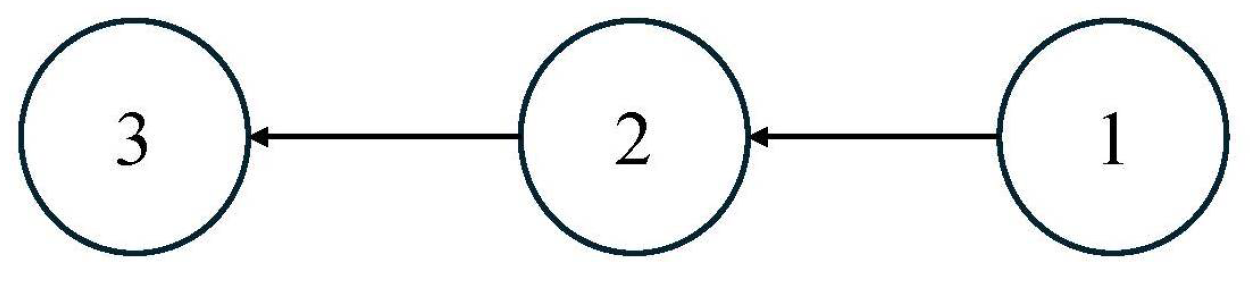
In this section, some mathematical preliminaries are presented, and the problem addressed in this paper is formulated.

2.1. Graph Theory

Define the directed graph $\mathcal{G}=(\mathcal{V},\mathcal{E},\mathcal{A})$, where $\mathcal{V}=\{{\mathfrak{v}}_1,{\mathfrak{v}}_2,...,{\mathfrak{v}}_N\}$, $\mathcal{E}\subseteq \mathcal{V}\times \mathcal{V}$, and $\mathcal{A}={\left[{\mathfrak{a}}_{\mathfrak{ij}}\right]}_{N\times N}$ are the set of nodes, the set of directed edges, and a weighted adjacency matrix, respectively. Define ${\mathfrak{a}}_{ij}>0$ if $({\mathfrak{v}}_j,{\mathfrak{v}}_i)\in \mathcal{E}$; otherwise, ${\mathfrak{a}}_{ij}=0$. The degree matrix is defined as $\mathcal{D}=\mathrm{diag}\{q_1,q_2,...,q_N\}$, where $q_i={\sum }_{j\in N_i}{\mathfrak{a}}_{ij}$. The Laplace matrix of a directed graph is $L=\mathcal{D}-\mathcal{A}$. Define $\mathcal{B}=\mathrm{diag}\{p_1,p_2,...,p_N\}$, and ${\mathfrak{v}}_0$ is the leader, $p_i=1$, if the i-th node can receive the leader’s information and $p_i=0$ otherwise.

2.2. Lemmas

For a generic dynamical system,

$$\begin{array}{c}\hfill \dot{x}=f\left(x\right),x\left(0\right)=x_0,\end{array}$$

(1)

where $x\in R^n$ and $f(·)$ are system states and nonlinear functions, respectively.

Lemma 1 

([9]). If there exists a positive definite function $V\left(x\right)$ and some parameters satisfying $\mathfrak{p}>0$, $\mathfrak{q}>0$, $0<\mathfrak{g}<1$, $\mathfrak{k}>1$, and $0<\varkappa <\infty$ such that

$$\begin{array}{c}\hfill \dot{V}\left(x\right)\le -\mathfrak{p}{V}^{\mathfrak{g}}\left(x\right)-\mathfrak{q}{V}^{\mathfrak{k}}\left(x\right)+\varkappa ,\end{array}$$

(2)

system (1) is referred to as being semiglobal practical fixed-time stable (SPFTS), and the states of system (1) can reach the following set within the interval $[0,{\mathcal{T}}_f]$:

$$\mathsf{\Omega }=\left\{x|V\left(x\right)\le min\left\{{\left({\displaystyle \frac{\varkappa }{\mathfrak{p}(1-\iota )}}\right)}^{{\displaystyle \frac{1}{\mathfrak{g}}}},{\left({\displaystyle \frac{\varkappa }{\mathfrak{q}(1-\iota )}}\right)}^{{\displaystyle \frac{1}{\mathfrak{k}}}}\right\}\right\},$$

(3)

where the scalar ι satisfies $0<\iota <1$, and the settling time ${\mathcal{T}}_f$ is bound by the fixed-time ${\mathcal{T}}_{\mathit{max}}$

$${\mathcal{T}}_f\le {\mathcal{T}}_{\mathit{max}}={\displaystyle \frac{1}{\mathfrak{p}\iota (1-\mathfrak{g})}}+{\displaystyle \frac{1}{\mathfrak{q}\iota (\mathfrak{k}-1)}}.$$

(4)

Lemma 2 

([24]). If ρ and ς are real variables and $\mathfrak{x}$, $\mathfrak{y}$, and $\mathfrak{z}$ are positive constants, we have

$${\left|\rho \right|}^{\mathfrak{x}}{\left|\varsigma \right|}^{\mathfrak{y}}\le {\displaystyle \frac{\mathfrak{x}}{\mathfrak{x}+\mathfrak{y}}}\mathfrak{z}{\left|\rho \right|}^{\mathfrak{x}+\mathfrak{y}}+{\displaystyle \frac{\mathfrak{y}}{\mathfrak{x}+\mathfrak{y}}}{\mathfrak{z}}^{-{\displaystyle \frac{\mathfrak{x}}{\mathfrak{y}}}}{\left|\varsigma \right|}^{\mathfrak{x}+\mathfrak{y}}.$$

(5)

Lemma 3 

([9]). For ${\lambda }_1,{\lambda }_2,...,{\lambda }_n\ge 0$ and $m>0$, if $0<m<1$, one can obtain ${\displaystyle \sum _{i=1}^n}{\lambda }_i^m\ge {\left({\displaystyle \sum _{i=1}^n}{\lambda }_i\right)}^m$; otherwise, one has ${\displaystyle \sum _{i=1}^n}{\lambda }_i^m\ge n^{1-m}{\left({\displaystyle \sum _{i=1}^n}{\lambda }_i\right)}^m$.

Lemma 4 

([44]). If $\delta \in R$ and $ϵ>0$, we have

$$\begin{array}{c}\hfill 0\le \left|\delta \right|-\delta tanh\left({\displaystyle \frac{\delta }{ϵ}}\right)\le 0.2785ϵ.\end{array}$$

(6)

Lemma 5 

([44]). For $\forall (\gamma ,\delta )\in R^2$, the following inequality holds:

$$\gamma \delta \le {\displaystyle \frac{{\eta }^{\mathfrak{g}}}{\mathfrak{g}}}{\left|\gamma \right|}^{\mathfrak{g}}+{\displaystyle \frac{1}{\mathfrak{h}{\eta }^{\mathfrak{h}}}}{\left|\delta \right|}^{\mathfrak{h}},$$

(7)

where $\eta >0,\mathfrak{g}>1,\mathfrak{h}>1$ and $(\mathfrak{g}-1)(\mathfrak{h}-1)=1$.

Lemma 6 

([9]). Radial basis function neural networks (RBF NNs) are often used to estimate the unknown terms of nonlinear systems due to their excellent approximation ability. An unknown smooth function $\mathcal{F}\left(Z\right)$ can be approximated by the following:

$$\mathcal{F}\left(Z\right)={\mathsf{\Lambda }}^{\mathrm{T}}\mathsf{\Xi }\left(Z\right),$$

(8)

where $\mathsf{\Lambda }={[w_1,...,w_l]}^{\mathrm{T}}\in R^l$ denotes the ideal weight vector, l denotes the node number in the hidden layer, $Z\in R^n$ is an input vector, $\mathsf{\Xi }\left(Z\right)=[{\xi }_1\left(Z\right),...,{\xi }_l\left(Z\right)]$ represents the basis function vector, and ${\xi }_i\left(Z\right)$ is the Gaussian basis function with the following form:

$${\xi }_i\left(Z\right)=exp\left(-{\displaystyle \frac{{\parallel X-{ϵ}_i\parallel }^2}{{\iota }_i^2}}\right),i=1,2,...,l,$$

(9)

with ${ϵ}_i$ denoting the center of the Gaussian kernel and ${\iota }_i$ representing the width of the Gaussian kernel.

As is well known, RBF NNs in (8) can uniformly estimate any discrete-time unknown functions with arbitrary accuracy. Further, the unknown function can be rewritten as follows:

$$\begin{array}{c}\hfill \mathcal{F}\left(Z\right)={\mathsf{\Lambda }}^{\mathrm{T}}\mathsf{\Xi }\left(Z\right)+\epsilon \left(Z\right),\end{array}$$

(10)

where $\mathsf{\Lambda }$ and $\epsilon \left(Z\right)$ are the ideal weight vector and estimation error, respectively.

2.3. Problem Statement

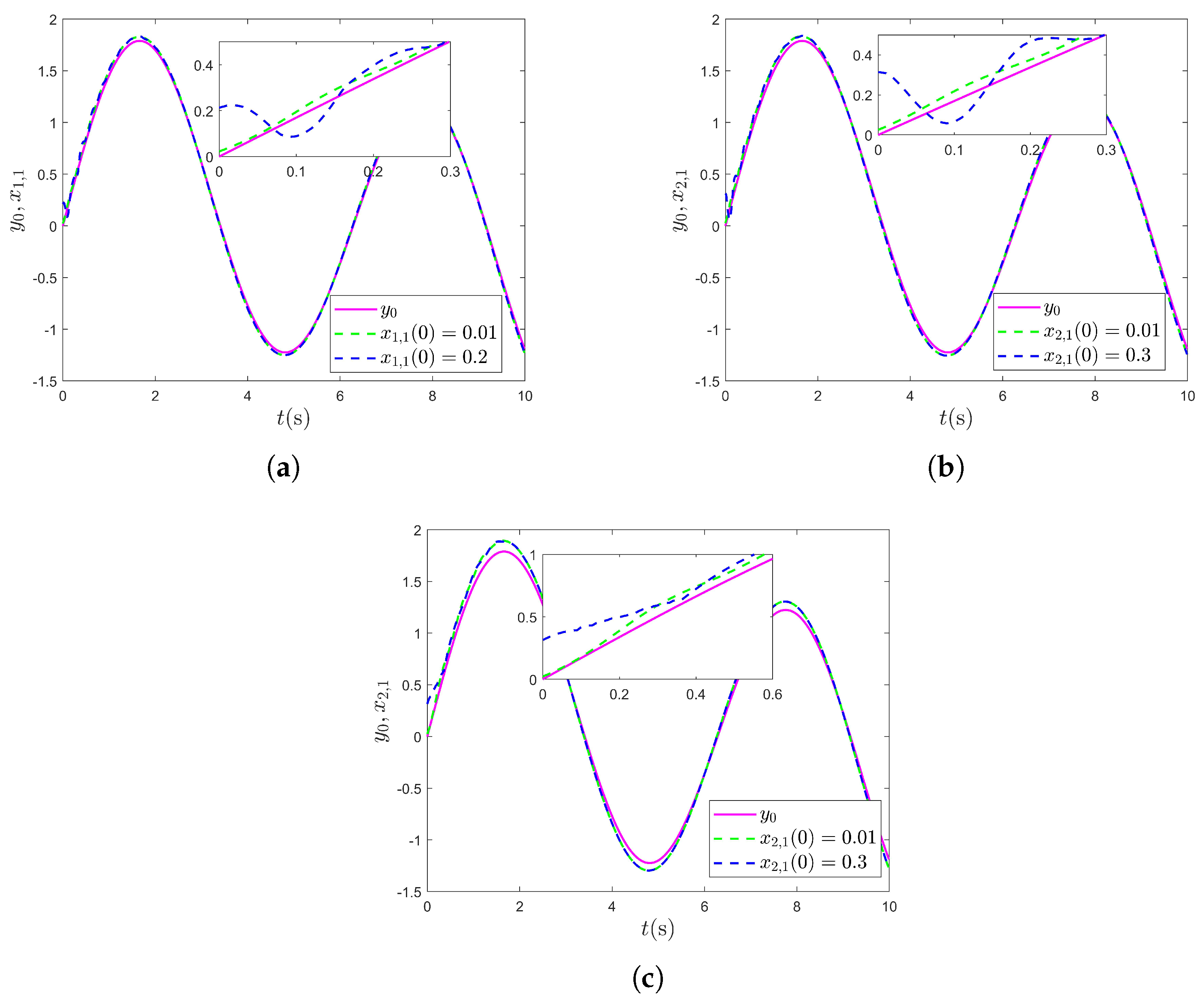
Consider the following high-order nonlinear multi-agent time delay system:

$$\begin{array}{c}\left\{\begin{array}{c}{\dot{x}}_{i,m}\left(t\right)=x_{i,m+1}\left(t\right)+{\mathfrak{L}}_{i,m}\left({\overline{x}}_{i,m}(t-{\tau }_{i,m})\right)+{\mathfrak{d}}_{i,m}\left({\overline{x}}_{i,m}\left(t\right)\right),\hfill \\ {\dot{x}}_{i,n_i}\left(t\right)=u_i\left(t\right)+{\mathfrak{L}}_{i,n_i}\left(x_{i,n_i}(t-{\tau }_{i,n_i})\right)+{\mathfrak{d}}_{i,n_i}\left(x_{i,n_i}\left(t\right)\right),\hfill \\ y_i=x_{i,1},i=1,\cdots ,N;m=1,\cdots ,n_i-1.\hfill \end{array}\right.\hfill \end{array},$$

(11)

where $x_i={[x_{i,1},x_{i,2},\cdots ,x_{i,n_i}]}^{\mathrm{T}}\in {\mathbb{R}}^{n_i}$, $u_i\left(t\right)\in \mathbb{R}$, and $y_i\in \mathbb{R}$ are the states, input, and output of the ith subsystem, respectively. ${\mathfrak{L}}_{i,m}\left({\overline{x}}_{i,m}(t-{\tau }_{i,m})\right)$ represents the unknown smooth nonlinear time delay function, ${\tau }_{i,m}$ is the unknown stochastic state delay, and ${\mathfrak{d}}_{i,m}\left({\overline{x}}_{i,m}\left(t\right)\right)$ is the external disturbance. Here, $x_i(t-{\tau }_{i,m})$ is written as $x_i\left({\tau }_{i,m}\right)$ for simplicity.

The main objective of this paper is to design the control input $u_i$ for the high-order nonlinear multi-agent time delay system (11) such that the following are true:

• The output $y_i$ can track the reference signal $y_0$ within a fixed time, and all the closed-loop signals are SPFTS.
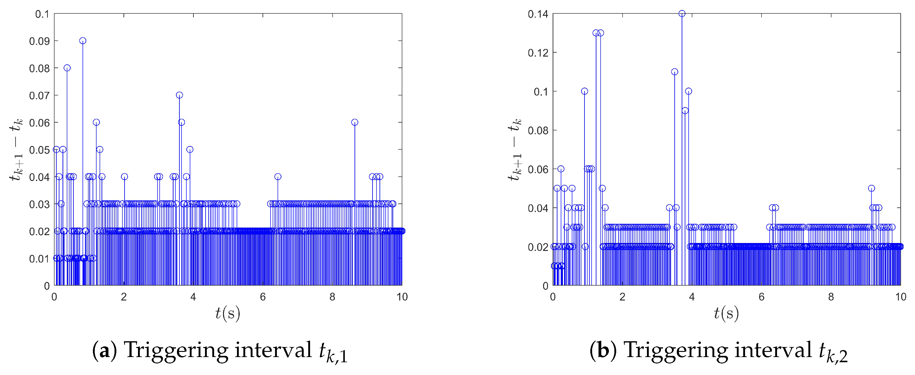
• The communication resources are significantly reduced with the introduction of the event-triggered mechanism.
• The system can remain stable in the presence of unknown stochastic time delays.

Here are several important assumptions for the subsequent controller design.

Assumption 1. 

The desired signal $y_0\left(t\right)$ and its mth-order derivatives $y_0^{\left(m\right)}(m=1,2,...,n)$ are continuous and bound.

Assumption 2. 

The time delay function ${\mathfrak{L}}_{i,m}\left({\overline{x}}_{i,m}\right)$ satisfies $\left|{\mathfrak{L}}_{i,m}\left({\overline{x}}_{i,m}\right)\right|\le {\sum }_{g=1}^m{\mathfrak{I}}_{i,m,g}\left(x_{i,g}\right)$, where ${\mathfrak{I}}_{i,m,g}\left(x_{i,g}\right)$ is an unknown bounded positive function.

Assumption 3. 

For an unknown positive function ${\mathfrak{I}}_{i,m,h}\left(x_{i,h}\right)$, we have the following inequalities:

$${\displaystyle \frac{1}{2}}\sum _{m=1}^{n_i}\sum _{v=1}^{n_i}\sum _{g=1}^v{\int }_{t-{\tau }_{i,v}}^t{\mathfrak{I}}_{i,v,g}^2\left(x_{i,g}\left(s\right)\right)ds=\mathfrak{b}\le \mathfrak{B},$$

(12)

$${\displaystyle \frac{1}{2}}\sum _{m=1}^{n_i}\sum _{j\in N_i}\sum _{v=1}^{n_i}\sum _{g=1}^v{\int }_{t-{\tau }_{i,v}}^t{\mathfrak{I}}_{j,v,g}^2\left(x_{j,g}\left(s\right)\right)ds=\mathfrak{c}\le \mathfrak{C},$$

(13)

where $\mathfrak{b},\mathfrak{c},\mathfrak{B},\mathfrak{C}$ are positive constants.

Assumption 4. 

The external disturbance ${\mathfrak{d}}_{i,m}\left({\overline{x}}_{i,m}\left(t\right)\right)$ satisfies $\left|{\mathfrak{d}}_{i,m}\left({\overline{x}}_{i,m}\left(t\right)\right)\right|\le \left|{\sigma }_{i,m}\left({\overline{x}}_{i,m}\left(t\right)\right)\right|$, where ${\sigma }_{i,m}\left({\overline{x}}_{i,m}\left(t\right)\right)$ is an unknown function.

Remark 1. 

It is important to emphasize that the above four assumptions presented in this paper are both essential and reasonable. Assumption 1 serves as a foundational premise and is extensively prevalent in the backstepping-based controller design of high-order nonlinear systems [9,13,17]. In addition, this assumption is also coherent with some practical systems, such as the double-rod hydraulic position servo system [47], the uncertain quadrotor UAV system [48], the unmanned underwater vehicle pole attitude control system [49], etc. Since the time delay functions in the system is bound, it is reasonable that Assumption 2 assumes the upper bound of the time delay function to be ${\sum }_{g=1}^m{\mathfrak{I}}_{i,m,g}\left(x_{i,g}\right)$. Additionally, it is clear that the integrals and summations of bound functions are also bound; thus, Assumption 3 is equally reasonable. Assumption 4 is widely validated by extensive experiments, as detailed in [50].

3. Main Results

The fixed-time event-triggered controller is constructed in this section, and the structure of the proposed strategy is displayed in Figure 1. Combining RBF NNs, the fixed-time stability theory, and the Lyapunov–Krasovskii functional, the virtual control law and adaptive law of the system are built by virtue of the backstepping technique. Then, the control signal is further obtained through the ETM, allowing for appropriate control of the system.

3.1. Event-Triggered Mechanism Design

Define ${\mathfrak{e}}_i\left(t\right)={\mathsf{\Psi }}_i\left(t\right)-{\mathsf{\Psi }}_i\left(t_k\right)$, where t and $t_k$ are the current time and the previous triggering time, and ${\mathsf{\Psi }}_i$ is the control signal. Then, the triggering event will only be executed when the following inequality holds:

$$\left|{\mathfrak{e}}_i\left(t\right)\right|\ge {\gamma }_i\left|{\mathsf{\Psi }}_i\left(t_k\right)\right|+{\eta }_i,$$

(14)

where ${\gamma }_i\in (0,1)$ and ${\eta }_i>0$ are two positive parameters.

Then, the triggering time $t_{k+1}$ can be expressed as follows:

$$t_{k+1}=inf\left\{t>t_k|\left|{\mathfrak{e}}_i\left(t\right)\right|\ge {\gamma }_i\left|{\mathsf{\Psi }}_i\left(t_k\right)\right|+{\eta }_i\right\}.$$

(15)

Then, we have the following formula:

$${\mathsf{\Psi }}_i\left(t\right)=\left(1+{\mathfrak{w}}_1\left(t\right){\gamma }_i\right)u_i\left(t\right)+{\mathfrak{w}}_2\left(t\right){\eta }_i,t\in \left[t_k,t_{k+1}\right),$$

(16)

where $u_i\left(t\right)$ is the control input, ${\eta }_i$ is a positive parameter, and ${\mathfrak{w}}_1\left(t\right)$ and ${\mathfrak{w}}_2\left(t\right)$ are time-varying parameters with $\left|{\mathfrak{w}}_1\left(t\right)\right|\le 1$ and $\left|{\mathfrak{w}}_2\left(t\right)\right|\le 1$.

Further, the actuator signal $u_i\left(t\right)$ can be written as follows:

$$u_i\left(t\right)={\displaystyle \frac{{\mathsf{\Psi }}_i\left(t\right)}{1+{\mathfrak{w}}_1\left(t\right){\gamma }_i}}-{\displaystyle \frac{{\mathfrak{w}}_2\left(t\right){\eta }_i}{1+{\mathfrak{w}}_1\left(t\right){\gamma }_i}}.$$

(17)

3.2. Fixed-Time Event-Triggered Controller Design Under Unknown Stochastic Time Delay

The tracking errors of each system are constructed as follows:

$$\begin{array}{c}\left\{\begin{array}{cc}\hfill & z_{i,1}=\sum _{j\in N_i}{\mathfrak{a}}_{i,j}(x_{i,1}-x_{j,1})+p_i(x_{i,1}-y_0),\hfill \\ \hfill & z_{i,r}=x_{i,r}-{\alpha }_{i,r-1},r=2,...,n_i.\hfill \end{array}\right.\hfill \end{array},$$

(18)

where ${\alpha }_{i,q}(q=1,2,...,n_i)$ is the virtual control law, and ${\mathfrak{a}}_{i,j}$ is the element of the adjacency matrix $\mathcal{A}$.

Step $i,1$: Construct the Lyapunov function as follows:

$$\begin{array}{cc}\hfill V_{i,1}& ={\displaystyle \frac{1}{2}}{z}_{i,1}^2+{\displaystyle \frac{1}{2}}{\int }_{t-{\tau }_{i,1}}^t{\mathfrak{I}}_{i,1,1}^2\left(x_{i,1}\left(s\right)\right)ds+{\displaystyle \frac{1}{2}}\sum _{j\in N_i}{\int }_{t-{\tau }_{i,1}}^t{\mathfrak{I}}_{j,1,1}^2\left(x_{j,1}\left(s\right)\right)ds.\hfill \end{array}$$

(19)

The derivative of $V_{i,1}$ is as follows:

$$\begin{array}{cc}\hfill {\dot{V}}_{i,1}=& z_{i,1}((p_i+q_i)(z_{i,2}+{\alpha }_{i,1}+{\mathfrak{L}}_{i,1}\left({\overline{x}}_{i,1}\left({\tau }_{i,1}\right)\right)+{\mathfrak{d}}_{i,1}\left({\overline{x}}_{i,1}\right))-\sum _{j\in N_i}{a}_{i,j}(x_{j,2}+{\mathfrak{L}}_{j,1}\left({\overline{x}}_{j,1}\left({\tau }_{j,1}\right)\right)\hfill \\ \hfill & {\displaystyle +{\mathfrak{d}}_{j,1}\left({\overline{x}}_{j,1}\left(t\right)\right))-p_i{\dot{y}}_0)+\frac{1}{2}{\mathfrak{I}}_{i,1,1}^2\left(x_{i,1}\left(t\right)\right)-\frac{1}{2}{\mathfrak{I}}_{i,1,1}^2\left(x_{i,1}\left({\tau }_{i,1}\right)\right)+\frac{1}{2}\sum _{j\in N_i}{\mathfrak{I}}_{j,1,1}^2\left(x_{j,1}\left(t\right)\right)}\hfill \\ \hfill & -{\displaystyle \frac{1}{2}}\sum _{j\in N_i}{\mathfrak{I}}_{j,1,1}^2\left(x_{j,1}\left({\tau }_{j,1}\right)\right).\hfill \end{array}$$

(20)

According to Lemma 5, one has the following:

$$z_{i,1}{\mathfrak{L}}_{i,1}\left({\overline{x}}_{i,1}\left({\tau }_{i,1}\right)\right)\le {\displaystyle \frac{(p_i+q_i)z_{i,1}^2}{2}}+{\displaystyle \frac{{\mathfrak{I}}_{i,1,1}^2\left(x_{i,1}\left({\tau }_{i,1}\right)\right)}{2(p_i+q_i)}},$$

(21)

$$z_{i,1}{\mathfrak{d}}_{i,1}\left(x_{i,1}\right)\le {\displaystyle \frac{(p_i+q_i)b_{i,0,0}^2}{2}}+{\displaystyle \frac{z_{i,1}^2{\sigma }_{i,1}^2}{2(p_i+q_i)b_{i,0,0}^2}},$$

(22)

$$z_{i,1}{\mathfrak{L}}_{j,1}\left({\overline{x}}_{j,1}\left({\tau }_{j,1}\right)\right)\le {\displaystyle \frac{z_{i,1}^2}{2}}+{\displaystyle \frac{{\mathfrak{I}}_{j,1,1}^2\left(x_{j,1}\left({\tau }_{j,1}\right)\right)}{2}},$$

(23)

$$z_{i,1}{\mathfrak{d}}_{j,1}\left(x_{j,1}\right)\le {\displaystyle \frac{b_{j,1,1}^2}{2}}+{\displaystyle \frac{z_{i,1}^2{\sigma }_{j,1}^2}{2b_{j,1,1}^2}},$$

(24)

where $b_{i,0,0}$ and $b_{j,1,1}$ are positive constants.

Substituting (21)–(24) into (20) yields the following:

$$\begin{array}{cc}\hfill {\dot{V}}_{i,1}\le & z_{i,1}[(p_i+q_i)(z_{i,2}+{\alpha }_{i,1})+{\displaystyle \frac{1}{2}}{z}_{i,1}{(p_i+q_i)}^2+{\displaystyle \frac{z_{i,1}{\sigma }_{i,1}^2}{2b_{i,0,0}^2}}-\sum _{j\in N_i}{a}_{i,j}(x_{j,2}-{\displaystyle \frac{1}{2}}{z}_{i,1}-{\displaystyle \frac{z_{i,1}{\sigma }_{j,1}^2}{2b_{j,1,1}^2}})\hfill \\ \hfill & -p_i{\dot{y}}_0]+{\displaystyle \frac{{(p_i+q_i)}^2{b}_{i,0,0}^2}{2}}+\sum _{j\in N_i}{\displaystyle \frac{b_{j,1,1}^2}{2}}+{\displaystyle \frac{1}{2}}{\mathfrak{I}}_{i,1,1}^2(x_{i,1}(t))+{\displaystyle \frac{1}{2}}\sum _{j\in N_i}{\mathfrak{I}}_{j,1,1}^2(x_{j,1}(t))\hfill \\ \hfill =& z_{i,1}[(p_i+q_i)(z_{i,2}+{\alpha }_{i,1})-\sum _{j\in N_i}{a}_{i,j}{x}_{j,2}-p_i{\dot{y}}_0+{\mathcal{F}}_{i,1}]+{\displaystyle \frac{b_{i,1,1}^2}{2}}+\sum _{j\in N_i}{\displaystyle \frac{b_{j,1,1}^2}{2}}\hfill \\ \hfill & +{\displaystyle \frac{1}{2}}{\mathfrak{I}}_{i,1,1}^2(x_{i,1}(t))+{\displaystyle \frac{1}{2}}\sum _{j\in N_i}{\mathfrak{I}}_{j,1,1}^2(x_{j,1}(t)),\hfill \end{array}$$

(25)

where ${\displaystyle {\mathcal{F}}_{i,1}=\frac{1}{2}{z}_{i,1}{(p_i+q_i)}^2+\frac{z_{i,1}{\sigma }_{i,1}^2}{2b_{i,0,0}^2}+\sum _{j\in N_i}{a}_{i,j}(\frac{1}{2}{z}_{i,1}+\frac{z_{i,1}{\sigma }_{j,1}^2}{2b_{j,1,1}^2})}$ and $b_{i,1,1}^2={(p_i+q_i)}^2{b}_{i,0,0}^2$.

According to Lemma 6, we have the following:

$${\mathcal{F}}_{i,1}={\mathsf{\Lambda }}_{i,1}^{\mathrm{T}}{\mathsf{\Xi }}_{i,1}+{\epsilon }_{i,1},$$

(26)

where $\left|{\epsilon }_{i,1}\right|\le {\mathfrak{g}}_{i,1}$ and ${\mathfrak{g}}_{i,1}>0$.

It can be inferred from Lemma 5 that

$$\begin{array}{c}\hfill z_{i,1}{\mathcal{F}}_{i,1}\le \left|z_{i,1}\right|\left(\parallel {\mathsf{\Lambda }}_{i,1}\parallel \parallel {\mathsf{\Xi }}_{i,1}\parallel +{\mathfrak{g}}_{i,1}\right)\le {\displaystyle \frac{z_{i,1}^2}{2c_{i,1}^2}}{\parallel {\mathsf{\Lambda }}_{i,1}\parallel }^2{\mathsf{\Xi }}_{i,1}^{\mathrm{T}}{\mathsf{\Xi }}_{i,1}+{\displaystyle \frac{1}{2}}{c_{i,1}}^2+{\displaystyle \frac{z_{i,1}^2}{2}}+{\displaystyle \frac{1}{2}}{\mathfrak{g}}_{i,1}^2,\end{array}$$

(27)

where $c_{i,1}$ is a positive parameter.

Define the estimation error ${\tilde{\theta }}_i$ as follows:

$${\tilde{\theta }}_i={\theta }_i-{\widehat{\theta }}_i,$$

(28)

where ${\theta }_i=max\left\{{\parallel {\mathsf{\Lambda }}_{i,j}\parallel }^2,j=1,2,...,n_i\right\}$, and ${\widehat{\theta }}_i$ is the estimation value of ${\theta }_i$.

Let ${\vartheta }_{i,r}>0$ and ${\nu }_{i,r}>0(r=1,2,...,n_i)$ be the designed parameters. Then, the virtual control law ${\alpha }_{i,1}$ can be designed as follows:

$$\begin{array}{cc}\hfill {\alpha }_{i,1}& ={\displaystyle \frac{1}{p_i+q_i}}\left(-{\vartheta }_{i,1}{z}_{i,1}^{2{\rho }_1-1}-{\nu }_{i,1}{z}_{i,1}^{2{\rho }_2-1}+\sum _{j\in N_i}{a}_{i,j}{x}_{j,2}-{\displaystyle \frac{1}{2}}{z}_{i,1}+p_i{\dot{y}}_0-{\displaystyle \frac{z_{i,1}}{2c_{i,1}^2}}{\widehat{\theta }}_i{\mathsf{\Xi }}_{i,1}^{\mathrm{T}}{\mathsf{\Xi }}_{i,1}\right).\hfill \end{array}$$

(29)

Substituting (26)–(29) into (25), we have

$$\begin{array}{cc}\hfill {\dot{V}}_{i,1}\le & -{\vartheta }_{i,1}{z}_{i,1}^{2{\rho }_1-1}-{\nu }_{i,1}{z}_{i,1}^{2{\rho }_2-1}+(p_i+q_i)z_{i,1}{z}_{i,2}+{\displaystyle \frac{z_{i,1}^2}{2c_{i,1}^2}}({\parallel {\mathsf{\Lambda }}_{i,1}\parallel }^2-{\widehat{\theta }}_i)S_{i,1}^{\mathrm{T}}{S}_{i,1}\hfill \\ \hfill & +{\displaystyle \frac{1}{2}}{\mathfrak{I}}_{i,1,1}^2\left(x_{i,1}\left(t\right)\right)+{\displaystyle \frac{1}{2}}\sum _{j\in N_i}{\mathfrak{I}}_{j,1,1}^2\left(x_{j,1}\left(t\right)\right)+{\displaystyle \frac{1}{2}}{c_{i,1}}^2+{\displaystyle \frac{1}{2}}{\mathfrak{g}}_{i,1}^2+{\displaystyle \frac{b_{i,1,1}^2}{2}}+\sum _{j\in N_i}{\displaystyle \frac{b_{j,1,1}^2}{2}}.\hfill \end{array}$$

(30)

Step $i,2$: Construct the Lyapunov function as follows:

$$\begin{array}{cc}\hfill V_{i,2}& =V_{i,1}+{\displaystyle \frac{1}{2}}{z}_{i,2}^2+{\displaystyle \frac{1}{2}}\sum _{v=1}^2\sum _{g=1}^v{\int }_{t-{\tau }_{i,v}}^t{\mathfrak{I}}_{i,v,g}^2\left(x_{i,g}\left(s\right)\right)ds+{\displaystyle \frac{1}{2}}\sum _{j\in N_i}\sum _{v=1}^2\sum _{g=1}^v{\int }_{t-{\tau }_{i,v}}^t{\mathfrak{I}}_{j,v,g}^2\left(x_{j,g}\left(s\right)\right)ds.\hfill \end{array}$$

(31)

The time derivative of (31) is as follows:

$$\begin{array}{cc}\hfill {\dot{V}}_{i,2}=& {\dot{V}}_{i,1}+z_{i,2}(z_{i,3}+{\alpha }_{i,2}+{\mathfrak{L}}_{i,2}\left({\overline{x}}_{i,2}\left({\tau }_{i,2}\right)\right)+{\mathfrak{d}}_{i,2}\left({\overline{x}}_{i,2}\right)-{\dot{\alpha }}_{i,1})+{\displaystyle \frac{1}{2}}\sum _{v=1}^2\sum _{g=1}^v[{\mathfrak{I}}_{i,v,g}^2\left(x_{i,g}\left(t\right)\right)\hfill \\ \hfill & -{\mathfrak{I}}_{i,v,g}^2\left(x_{i,g}\left({\tau }_{i,v}\right)\right)]+{\displaystyle \frac{1}{2}}\sum _{j\in N_i}\sum _{v=1}^2\sum _{g=1}^k\left[{\mathfrak{I}}_{j,v,g}^2\left(x_{j,g}\left(t\right)\right)-{\mathfrak{I}}_{j,v,g}^2\left(x_{j,g}\left({\tau }_{i,v}\right)\right)\right].\hfill \end{array}$$

(32)

Based on Lemma 5, one has the following:

$$z_{i,2}{\mathfrak{L}}_{i,2}\left({\overline{x}}_{i,2}\left({\tau }_{i,2}\right)\right)\le {\displaystyle \frac{z_{i,2}^2}{2}}+{\displaystyle \frac{1}{2}}\sum _{g=1}^2{\mathfrak{I}}_{i,2,g}^2\left(x_{i,g}\left({\tau }_{i,2}\right)\right),$$

(33)

$$z_{i,2}{\mathfrak{d}}_{i,2}\left({\overline{x}}_{i,2}\right)\le {\displaystyle \frac{b_{i,2,2}^2}{2}}+{\displaystyle \frac{z_{i,2}^2{\sigma }_{i,2}^2\left({\overline{x}}_{i,2}\right)}{2b_{i,2,2}^2}},$$

(34)

where $b_{i,2,2}$ is a positive constant.

The time derivative of ${\alpha }_{i,1}$ is as follows:

$$\begin{array}{cc}\hfill {\dot{\alpha }}_{i,1}& ={\displaystyle \frac{\partial {\alpha }_{i,1}}{\partial x_{i,1}}}{\dot{x}}_{i,1}+\sum _{j\in N_i}\sum _{v=1}^2{\displaystyle \frac{\partial {\alpha }_{i,1}}{\partial x_{j,v}}}{\dot{x}}_{j,v}+{\displaystyle \frac{\partial {\alpha }_{i,1}}{\partial {\widehat{\theta }}_i}}{\dot{\widehat{\theta }}}_i+\sum _{v=0}^1{\displaystyle \frac{\partial {\alpha }_{i,1}}{\partial y_0^{\left(v\right)}}}{\dot{y}}_0^{(v+1)}\hfill \\ \hfill & ={\mathcal{R}}_1+{\displaystyle \frac{\partial {\alpha }_{i,1}}{\partial x_{i,1}}}({\mathfrak{L}}_{i,1}\left(x_{i,1}\left({\tau }_{i,1}\right)\right)+{\mathfrak{d}}_{i,1}\left({\overline{x}}_{i,1}\right))+\sum _{j\in N_i}\sum _{v=1}^2{\displaystyle \frac{\partial {\alpha }_{i,1}}{\partial x_{j,v}}}({\mathfrak{L}}_{j,v}\left({\overline{x}}_{j,v}\left({\tau }_{j,v}\right)\right)+{\mathfrak{d}}_{j,v}\left({\overline{x}}_{j,v}\right)),\hfill \end{array}$$

(35)

where ${\displaystyle {\mathcal{R}}_1=\frac{\partial {\alpha }_{i,1}}{\partial x_{i,1}}{x}_{i,2}+\sum _{j\in N_i}\sum _{v=1}^2\frac{\partial {\alpha }_{i,1}}{\partial x_{j,v}}{x}_{j,v+1}+\frac{\partial {\alpha }_{i,1}}{\partial {\widehat{\theta }}_i}{\dot{\widehat{\theta }}}_i+\sum _{v=0}^1\frac{\partial {\alpha }_{i,1}}{\partial y_0^{\left(v\right)}}{\dot{y}}_0^{(v+1)}}$.

According to Lemma 5, one has the following:

$$\begin{array}{cc}\hfill -z_{i,2}{\displaystyle \frac{\partial {\alpha }_{i,1}}{\partial x_{i,1}}}{\mathfrak{L}}_{i,1}\left({\overline{x}}_{i,1}\left({\tau }_{i,1}\right)\right)& \le {\displaystyle \frac{z_{i,2}^2}{2}}{\left({\displaystyle \frac{\partial {\alpha }_{i,1}}{\partial x_{i,1}}}\right)}^2+{\displaystyle \frac{1}{2}}{\mathfrak{I}}_{i,1,1}^2\left(x_{i,1}\left({\tau }_{i,1}\right)\right),\hfill \end{array}$$

(36)

$$-z_{i,2}{\displaystyle \frac{\partial {\alpha }_{i,1}}{\partial x_{i,1}}}{\mathfrak{d}}_{i,1}\left(x_{i,1}\right)\le {\displaystyle \frac{z_{i,2}^2{\sigma }_{i,1}^2}{2b_{i,2,1}^2}}+{\displaystyle \frac{1}{2}}{b}_{i,2,1}^2,$$

(37)

$$\begin{array}{cc}\hfill -z_{i,2}\sum _{j\in N_i}& \sum _{v=1}^2{\displaystyle \frac{\partial {\alpha }_{i,1}}{\partial x_{j,v}}}{\mathfrak{L}}_{j,v}\left({\overline{x}}_{j,v}\left({\tau }_{j,v}\right)\right)\le \sum _{j\in N_i}\sum _{v=1}^2\left({\displaystyle \frac{z_{i,2}^2}{2}}{\left({\displaystyle \frac{\partial {\alpha }_{i,1}}{\partial x_{j,v}}}\right)}^2+{\displaystyle \frac{1}{2}}\sum _{g=1}^v{\mathfrak{I}}_{j,v,g}^2\left(x_{j,g}\left({\tau }_{j,v}\right)\right)\right),\hfill \end{array}$$

(38)

$$\begin{array}{cc}\hfill -z_{i,2}\sum _{j\in N_i}\sum _{v=1}^2{\displaystyle \frac{\partial {\alpha }_{i,1}}{\partial x_{j,v}}}{\mathfrak{d}}_{j,v}\left({\overline{x}}_{j,v}\right)& \le \sum _{j\in N_i}\sum _{v=1}^2\left({\displaystyle \frac{z_{i,2}^2{\sigma }_{j,v}^2}{2b_{j,2,v}^2}}{\left({\displaystyle \frac{\partial {\alpha }_{i,1}}{\partial x_{j,v}}}\right)}^2+{\displaystyle \frac{1}{2}}{b}_{j,2,v}^2\right).\hfill \end{array}$$

(39)

Substituting (33)–(39) into (32) yields the following:

$$\begin{array}{c}{\displaystyle {\dot{V}}_{i,2}\le {\dot{V}}_{i,1}+z_{i,2}\left(z_{i,3}+{\alpha }_{i,2}-{\mathcal{R}}_1\right)+\frac{1}{2}{z}_{i,2}^2+\frac{1}{2}\sum _{g=1}^2{\mathfrak{I}}_{i,2,g}^2(x_{i,h}\left({\tau }_{i,2}\right)+\frac{b_{i,2,2}^2}{2}+\frac{z_{i,2}^2{\sigma }_{i,2}^2\left({\overline{x}}_{i,2}\right)}{2b_{i,2,2}^2}}\hfill \\ {\displaystyle +\frac{z_{i,2}^2}{2}{\left(\frac{\partial {\alpha }_{i,1}}{\partial x_{i,1}}\right)}^2+\frac{1}{2}{\mathfrak{I}}_{i,1,1}^2\left(x_{i,1}\left({\tau }_{i,1}\right)\right)+\frac{z_{i,2}^2{\sigma }_{i,1}^2}{2b_{i,2,1}^2}+\frac{1}{2}{b}_{i,2,1}^2+\sum _{j\in N_i}\sum _{v=1}^2(\frac{z_{i,2}^2}{2}{\left(\frac{\partial {\alpha }_{i,1}}{\partial x_{j,v}}\right)}^2}\hfill \\ {\displaystyle +\frac{1}{2}\sum _{g=1}^v{\mathfrak{I}}_{j,v,g}^2{x}_{j,g}\left({\tau }_{j,v}\right))+\sum _{j\in N_i}\sum _{v=1}^2\left(\frac{z_{i,2}^2{\sigma }_{j,v}^2}{2b_{j,2,v}^2}{\left(\frac{\partial {\alpha }_{i,1}}{\partial x_{j,v}}\right)}^2+\frac{1}{2}{b}_{j,2,v}^2\right)}\hfill \\ {\displaystyle +\frac{1}{2}\sum _{v=1}^2\sum _{h=1}^v\left[{\mathfrak{I}}_{i,v,g}^2\left(x_{i,g}\left(t\right)\right)-{\mathfrak{I}}_{i,v,g}^2\left(x_{i,g}\left({\tau }_{i,v}\right)\right)\right]}\hfill \\ {\displaystyle +\frac{1}{2}\sum _{j\in N_i}\sum _{v=1}^2\sum _{g=1}^v\left[{\mathfrak{I}}_{j,v,g}^2\left(x_{j,g}\left(t\right)\right)-{\mathfrak{I}}_{j,v,g}^2\left(x_{j,g}\left({\tau }_{i,v}\right)\right)\right]}\hfill \\ {\displaystyle ={\dot{V}}_{i,1}+z_{i,2}\left(z_{i,3}+{\alpha }_{i,2}+{\mathcal{F}}_{i,2}\right)+\frac{1}{2}{z}_{i,2}^2+\frac{b_{i,2,2}^2}{2}+\frac{1}{2}{b}_{i,2,1}^2+\sum _{j\in N_i}\sum _{v=1}^2\frac{1}{2}{b}_{j,2,v}^2}\hfill \\ {\displaystyle +\frac{1}{2}\sum _{v=1}^2\sum _{g=1}^v{\mathfrak{I}}_{i,v,g}^2\left(x_{i,g}\left(t\right)\right)+\frac{1}{2}\sum _{j\in N_i}\sum _{v=1}^2\sum _{g=1}^v{\mathfrak{I}}_{j,v,g}^2\left(x_{j,g}\left(t\right)\right)}\hfill \end{array},$$

(40)

where ${\displaystyle {\mathcal{F}}_{i,2}=\frac{z_{i,2}{\sigma }_{i,2}^2\left({\overline{x}}_{i,2}\right)}{2b_{i,2,2}^2}+\frac{z_{i,2}}{2}{\left(\frac{\partial {\alpha }_{i,1}}{\partial x_{i,1}}\right)}^2+\sum _{j\in N_i}\sum _{v=1}^2\left(\frac{z_{i,2}}{2}{\left(\frac{\partial {\alpha }_{i,1}}{\partial x_{j,v}}\right)}^2+\frac{z_{i,2}{\sigma }_{j,k}^2}{2b_{j,2,v}^2}{\left(\frac{\partial {\alpha }_{i,1}}{\partial x_{j,v}}\right)}^2\right)+\frac{z_{i,2}{\sigma }_{i,1}^2}{2b_{i,2,1}^2}-{\mathcal{R}}_1}$.

According to Lemma 6, we have the following:

$${\mathcal{F}}_{i,2}={\mathsf{\Lambda }}_{i,2}^{\mathrm{T}}{\mathsf{\Xi }}_{i,2}+{\epsilon }_{i,2},$$

(41)

where $\left|{\epsilon }_{i,2}\right|\le {\mathfrak{g}}_{i,2}$ and ${\mathfrak{g}}_{i,2}>0$.

Similar to (27), one has

$$\begin{array}{c}{\displaystyle z_{i,2}{\mathcal{F}}_{i,2}\le \left|z_{i,2}\right|\left(\parallel {\mathsf{\Lambda }}_{i,2}\parallel \parallel {\mathsf{\Xi }}_{i,2}\parallel +{\mathfrak{g}}_{i,2}\right)\le \frac{z_{i,2}^2}{2c_{i,2}^2}{\parallel {\mathsf{\Lambda }}_{i,2}\parallel }^2{\mathsf{\Xi }}_{i,2}^{\mathrm{T}}{\mathsf{\Xi }}_{i,2}+\frac{1}{2}{c_{i,2}}^2+\frac{z_{i,2}^2}{2}+\frac{1}{2}{\mathfrak{g}}_{i,2}^2}\hfill \end{array},$$

(42)

where $c_{i,2}$ is a positive parameter.

Similar to (29), ${\alpha }_{i,2}$ can be designed as follows:

$$\begin{array}{c}\hfill {\alpha }_{i,2}=-{\vartheta }_{i,2}{z}_{i,2}^{2{\rho }_1-1}-{\nu }_{i,2}{z}_{i,2}^{2{\rho }_2-1}-z_{i,2}+(p_i+q_i)z_{i,1}-{\displaystyle \frac{z_{i,2}}{2c_{i,2}^2}}{\widehat{\theta }}_i{\mathsf{\Xi }}_{i,2}^{\mathrm{T}}{\mathsf{\Xi }}_{i,2}.\end{array}$$

(43)

Substituting (41)–(43) into (40) yields the following:

$$\begin{array}{cc}\hfill {\dot{V}}_{i,2}\le & -\sum _{m=1}^2{\vartheta }_{i,m}{z}_{i,m}^{2{\rho }_1}-\sum _{m=1}^2{\nu }_{i,m}{z}_{i,m}^{2{\rho }_2}+z_{i,2}{z}_{i,3}+\sum _{m=1}^2{\displaystyle \frac{z_{i,m}^2}{2c_{i,m}^2}}\left({\parallel {\mathsf{\Lambda }}_{i,m}\parallel }^2-\widehat{{\theta }_i}\right)S_{i,2}^{\mathrm{T}}{S}_{i,2}\hfill \\ \hfill & +{\displaystyle \frac{1}{2}}\sum _{m=1}^2\sum _{v=1}^m\sum _{g=1}^k\left({\mathfrak{I}}_{i,v,g}^2\left(x_{i,g}\left(t\right)\right)+\sum _{j\in N_i}{\mathfrak{I}}_{j,v,g}^2\left(x_{j,g}\left(t\right)\right)\right)+{\displaystyle \frac{1}{2}}\sum _{m=1}^2\left(c_{i,m}^2+{\mathfrak{g}}_{i,m}^2\right)\hfill \\ \hfill & +{\displaystyle \frac{1}{2}}\sum _{v=1}^2\sum _{g=1}^v\left(b_{i,v,g}^2+\sum _{j\in N_i}{b}_{j,v,g}^2\right).\hfill \end{array}$$

(44)

Step $i,r(r=3,...,n_i-1)$: Design the Lyapunov function as follows:

$$\begin{array}{cc}\hfill V_{i,r}& =V_{i,r-1}+{\displaystyle \frac{1}{2}}{z}_{i,r}^2+{\displaystyle \frac{1}{2}}\sum _{v=1}^r\sum _{g=1}^v{\int }_{t-{\tau }_{i,v}}^t{\mathfrak{I}}_{i,v,g}^2\left(x_{i,g}\left(s\right)\right)ds+{\displaystyle \frac{1}{2}}\sum _{j\in N_i}\sum _{v=1}^r\sum _{g=1}^v{\int }_{t-{\tau }_{j,v}}^t{\mathfrak{I}}_{j,v,g}^2\left(x_{j,g}\left(s\right)\right)ds.\hfill \end{array}$$

(45)

Similar to (43), we have

$$\begin{array}{cc}\hfill {\alpha }_{i,r}& =-{\vartheta }_{i,r}{z}_{i,r}^{2{\rho }_1-1}-{\nu }_{i,r}{z}_{i,r}^{2{\rho }_2-1}-z_{i,r}-z_{i,r-1}-{\displaystyle \frac{z_{i,r}}{2c_{i,r}^2}}{\widehat{\theta }}_i{\mathsf{\Xi }}_{i,r}^{\mathrm{T}}{\mathsf{\Xi }}_{i,r}.\hfill \end{array}$$

(46)

Then, the following inequality can be obtained:

$$\begin{array}{cc}\hfill {\dot{V}}_{i,r}\le & -\sum _{m=1}^r{\vartheta }_{i,m}{z}_{i,m}^{2{\rho }_1}-\sum _{m=1}^r{\nu }_{i,m}{z}_{i,m}^{2{\rho }_2}+z_{i,r}{z}_{i,r+1}+\sum _{m=1}^r{\displaystyle \frac{z_{i,m}^2}{2c_{i,m}^2}}\left({\parallel {\mathsf{\Lambda }}_{i,m}\parallel }^2-\widehat{{\theta }_i}\right){\mathsf{\Xi }}_{i,m}^{\mathrm{T}}{\mathsf{\Xi }}_{i,m}\hfill \\ \hfill & +{\displaystyle \frac{1}{2}}\sum _{m=1}^r\sum _{v=1}^m\sum _{g=1}^v\left({\mathfrak{I}}_{i,v,g}^2\left(x_{i,g}\left(t\right)\right)+\sum _{j\in N_i}{\mathfrak{I}}_{j,v,g}^2\left(x_{j,g}\left(t\right)\right)\right)+{\displaystyle \frac{1}{2}}\sum _{m=2}^r(c_{i,m}^2+{\mathfrak{g}}_{i,m}^2)\hfill \\ \hfill & +{\displaystyle \frac{1}{2}}\sum _{v=1}^r\sum _{g=1}^v\left(b_{i,v,g}^2+\sum _{j\in N_i}{b}_{j,v,g}^2\right).\hfill \end{array}$$

(47)

Step $i,n_i$: The Lyapunov function can be constructed as follows:

$$\begin{array}{cc}\hfill V_{i,n_i}=& V_{i,n_i-1}+{\displaystyle \frac{1}{2}}\sum _{v=1}^{n_i}\sum _{g=1}^v{\int }_{t-{\tau }_{i,v}}^t{\mathfrak{I}}_{i,v,g}^2\left(x_{i,g}\left(s\right)\right)ds+{\displaystyle \frac{1}{2}}\sum _{j\in N_i}\sum _{v=1}^{n_i}\sum _{g=1}^v{\int }_{t-{\tau }_{j,v}}^t{\mathfrak{I}}_{j,v,g}^2\left(x_{j,g}\left(s\right)\right)ds\hfill \\ \hfill & +{\displaystyle \frac{1}{2}}{\tilde{\theta }}_i^2+{\displaystyle \frac{1}{2}}{z}_{i,n_i}^2.\hfill \end{array}$$

(48)

The time derivative of the above function is as follows:

$$\begin{array}{cc}\hfill {\dot{V}}_{i,n_i}=& {\dot{V}}_{i,n_i-1}+z_{i,n_i}(u_i+{\mathfrak{L}}_{i,n_i}\left({\overline{x}}_{i,n_i}\left({\tau }_{i,n_i}\right)\right)+{\mathfrak{d}}_{i,n_i}\left({\overline{x}}_{i,n_i}\right)-{\dot{\alpha }}_{i,n_i-1})-\widetilde{{\theta }_i}\dot{\widehat{{\theta }_i}}\hfill \\ \hfill & +{\displaystyle \frac{1}{2}}\sum _{v=1}^{n_i}\sum _{g=1}^v\left({\mathfrak{I}}_{i,v,g}^2\left(x_{i,g}\left(t\right)\right){\mathfrak{I}}_{i,v,g}^2\left(x_{i,g}\left({\tau }_{i,v}\right)\right)\right)+{\displaystyle \frac{1}{2}}\sum _{j\in N_i}\sum _{v=1}^2\sum _{g=1}^{n_i}({\mathfrak{I}}_{j,v,g}^2\left(x_{j,g}\left(t\right)\right)\hfill \\ \hfill & -\sum _{j\in N_i}{\mathfrak{I}}_{j,v,g}^2\left(x_{j,g}\left({\tau }_{i,v}\right)\right)).\hfill \end{array}$$

(49)

Combining Lemma 5, we have the following inequalities:

$$z_{i,n_i}{\mathfrak{L}}_{i,n_i}\left({\overline{x}}_{i,n_i}\left({\tau }_{i,n_i}\right)\right)\le {\displaystyle \frac{z_{i,n_i}^2}{2}}+{\displaystyle \frac{1}{2}}\sum _{g=1}^{n_i}{\mathfrak{I}}_{i,n_i,g}^2(x_{i,n_i}\left({\tau }_{i,n_i}\right),$$

(50)

$$z_{i,n_i}{\mathfrak{d}}_{i,n_i}\left({\overline{x}}_{i,n_i}\right)\le {\displaystyle \frac{b_{i,n_i,n_i}^2}{2}}+{\displaystyle \frac{z_{i,n_i}^2{\sigma }_{i,n_i}^2\left({\overline{x}}_{i,n_i}\right)}{2b_{i,n_i,n_i}^2}},$$

(51)

where $b_{i,n_i,n_i}$ is a positive constant.

The derivative of ${\alpha }_{i,n_i-1}$ is as follows:

$$\begin{array}{cc}\hfill {\dot{\alpha }}_{i,n_i-1}=& {\mathcal{R}}_{n_i-1}+\sum _{v=1}^{n_i-1}{\displaystyle \frac{\partial {\alpha }_{i,n_i-1}}{\partial x_{i,v}}}\left({\mathfrak{L}}_{i,v}\left({\overline{x}}_{i,v}\left({\tau }_{i,v}\right)\right)+{\mathfrak{d}}_{i,v}\left({\overline{x}}_{i,v}\right)\right)+\sum _{v=1}^{n_i}\sum _{j\in N_i}{\displaystyle \frac{\partial {\alpha }_{i,n_i-1}}{\partial x_{j,v}}}({\mathfrak{L}}_{j,v}\left({\overline{x}}_{j,v}\left({\tau }_{j,v}\right)\right)\hfill \\ \hfill & +{\mathfrak{d}}_{j,v}\left({\overline{x}}_{j,v}\right)),\hfill \end{array}$$

(52)

where ${\displaystyle {\mathcal{R}}_{n_i-1}=\sum _{v=1}^{n_i-1}\frac{\partial {\alpha }_{i,n_i-1}}{\partial x_{i,v}}{x}_{i,v+1}+\sum _{v=1}^{n_i}\sum _{j\in N_i}\frac{\partial {\alpha }_{i,n_i-1}}{\partial x_{j,v}}{x}_{j,v+1}+\sum _{v=0}^{n_i-1}\frac{\partial {\alpha }_{i,n_i-1}}{\partial y_0^{\left(v\right)}}{y}_0^{(v+1)}+\frac{\partial {\alpha }_{i,n_i-1}}{\partial {\widehat{\theta }}_i}{\dot{\widehat{\theta }}}_i}$.

According to Lemma 5, one has

$$\begin{array}{cc}\hfill -\sum _{k=1}^{n_i-1}{z}_{i,n_i}& {\displaystyle \frac{\partial {\alpha }_{i,n_i-1}}{\partial x_{i,v}}}{\mathfrak{L}}_{i,v}\left({\overline{x}}_{i,v}\left({\tau }_{i,v}\right)\right)\le \sum _{v=1}^{n_i-1}\left({\displaystyle \frac{z_{i,n_i}^2}{2}}{\left({\displaystyle \frac{\partial {\alpha }_{i,n_i-1}}{\partial x_{i,v}}}\right)}^2+{\displaystyle \frac{1}{2}}\sum _{g=1}^v{\mathfrak{I}}_{i,v,g}^2\left({\overline{x}}_{i,v}\left({\tau }_{i,v}\right)\right)\right),\hfill \end{array}$$

(53)

$$-\sum _{v=1}^{n_i-1}{z}_{i,n_i}{\displaystyle \frac{\partial {\alpha }_{i,n_i-1}}{\partial x_{i,v}}}{\mathfrak{d}}_{i,v}\left({\overline{x}}_{i,v}\right)\le \sum _{v=1}^{n_i-1}\left({\displaystyle \frac{z_{i,n_i}^2{\sigma }_{i,v}^2}{2b_{i,n_i,v}^2}}+{\displaystyle \frac{1}{2}}{b}_{i,n_i,v}^2\right),$$

(54)

$$\begin{array}{cc}\hfill & -\sum _{j\in N_i}\sum _{v=1}^{n_i}{z}_{i,n_i}{\displaystyle \frac{\partial {\alpha }_{i,n_i-1}}{\partial x_{j,v}}}{\mathfrak{L}}_{j,v}\left({\overline{x}}_{j,v}\left({\tau }_{j,v}\right)\right)\le \sum _{j\in N_i}\sum _{v=1}^{n_i}\left({\displaystyle \frac{z_{i,n_i}^2}{2}}{\left({\displaystyle \frac{\partial {\alpha }_{i,n_i-1}}{\partial x_{j,v}}}\right)}^2+{\displaystyle \frac{1}{2}}\sum _{g=1}^v{\mathfrak{I}}_{j,v,g}^2\left({\overline{x}}_{j,g}\left({\tau }_{j,v}\right)\right)\right),\hfill \end{array}$$

(55)

$$\begin{array}{cc}\hfill -\sum _{j\in N_i}\sum _{v=1}^2{z}_{i,n_i}& {\displaystyle \frac{\partial {\alpha }_{i,n_i-1}}{\partial x_{j,v}}}{\mathfrak{d}}_{j,v}\left({\overline{x}}_{j,v}\right)\le \sum _{j\in N_i}\sum _{v=1}^{n_i}\left({\displaystyle \frac{z_{i,n_i}^2{\sigma }_{j,v}^2}{2b_{j,n_i,k}^2}}{\left({\displaystyle \frac{\partial {\alpha }_{i,n_i-1}}{\partial x_{j,v}}}\right)}^2+{\displaystyle \frac{1}{2}}{b}_{j,n_i,v}^2\right).\hfill \end{array}$$

(56)

Substituting (50)–(56) into (49), the following inequality can be obtained:

$$\begin{array}{cc}\hfill {\dot{V}}_{i,n_i}\le & {\dot{V}}_{i,n_i-1}+z_{i,n_i}\left(u_i\left(t\right)+{\mathcal{F}}_{i,n_i}\right)-{\tilde{\theta }}_i{\dot{\widehat{\theta }}}_i+{\displaystyle \frac{1}{2}}{z}_{i,n_i}^2+{\displaystyle \frac{b_{i,n_i,n_i}^2}{2}}+{\displaystyle \frac{1}{2}}\sum _{v=1}^{n_i-1}{b}_{i,n_i,v}^2+\sum _{j\in N_i}\sum _{v=1}^{n_i}{\displaystyle \frac{1}{2}}{b}_{j,n_i,v}^2\hfill \\ \hfill & +{\displaystyle \frac{1}{2}}\sum _{v=1}^{n_i}\sum _{g=1}^v{\mathfrak{I}}_{i,v,g}^2\left(x_{i,g}\left(t\right)\right)+{\displaystyle \frac{1}{2}}\sum _{j\in N_i}\sum _{v=1}^{n_i}\sum _{g=1}^v{\mathfrak{I}}_{j,v,g}^2\left(x_{j,g}\left(t\right)\right),\hfill \end{array}$$

(57)

where ${\displaystyle {\mathcal{F}}_{i,n_i}=\frac{z_{i,n_i}{\sigma }_{i,n_i}^2\left({\overline{x}}_{i,n_i}\right)}{2b_{i,n_i,n_i}^2}+\sum _{j\in N_i}\sum _{v=1}^{n_i}\left(\frac{z_{i,n_i}^2}{2}{\left(\frac{\partial {\alpha }_{i,n_i-1}}{\partial x_{j,v}}\right)}^2+\frac{z_{i,n_i}{\sigma }_{j,v}^2}{2b_{j,n_i,v}^2}{\left(\frac{\partial {\alpha }_{i,n_i-1}}{\partial x_{j,v}}\right)}^2\right)+\sum _{v=1}^{n_i-1}\frac{z_{i,n_i}}{2}{\left(\frac{\partial {\alpha }_{i,n_i-1}}{\partial x_{i,v}}\right)}^2\sum _{v=1}^{n_i-1}\frac{z_{i,n_i}{\sigma }_{i,v}^2}{2b_{i,n_i,v}^2}-{\mathcal{R}}_{n_i-1}}$.

According to Lemma 6, we can obtain the following:

$${\mathcal{F}}_{i,n_i}={\mathsf{\Lambda }}_{i,n_i}^{\mathrm{T}}{\mathsf{\Xi }}_{i,n_i}+{\epsilon }_{i,n_i},$$

(58)

where $\left|{\epsilon }_{i,n_i}\right|\le {\mathfrak{g}}_{i,n_i}$ and ${\mathfrak{g}}_{i,n_i}>0$.

Based on Lemma 5, we have

$$\begin{array}{c}\hfill z_{i,n_i}{\mathcal{F}}_{i,n_i}\le \left|z_{i,n_i}\right|\left(\parallel {\mathsf{\Lambda }}_{i,n_i}\parallel \parallel {\mathsf{\Xi }}_{i,n_i}\parallel +{\mathfrak{g}}_{i,n_i}\right)\le {\displaystyle \frac{z_{i,n_i}^2}{2c_{i,n_i}^2}}{\parallel {\mathsf{\Lambda }}_{i,n_i}\parallel }^2{\mathsf{\Xi }}_{i,n_i}^{\mathrm{T}}{\mathsf{\Xi }}_{i,n_i}+{\displaystyle \frac{1}{2}}{c_{i,n_i}}^2+{\displaystyle \frac{z_{i,n_i}^2}{2}}+{\displaystyle \frac{1}{2}}{\mathfrak{g}}_{i,n_i}^2,\end{array}$$

(59)

where $c_{i,n_i}$ is a designed parameter.

Construct the virtual control law ${\alpha }_{i,n_i}$ as follows:

$$\begin{array}{c}\hfill {\alpha }_{i,n_i}=-{\vartheta }_{i,n_i}{z}_{i,n_i}^{2{\rho }_1-1}-{\nu }_{i,n_i}{z}_{i,n_i}^{2{\rho }_2-1}-z_{i,n_i}-z_{i,n_i-1}-{\displaystyle \frac{z_{i,n_i}}{2c_{i,n_i}^2}}{\widehat{\theta }}_i{\mathsf{\Xi }}_{i,n_i}^{\mathrm{T}}{\mathsf{\Xi }}_{i,n_i}.\end{array}$$

(60)

Substituting (58)–(60) into (57), one has

$$\begin{array}{cc}\hfill {\dot{V}}_{i,n_i}\le & -\sum _{m=1}^{n_i}{\vartheta }_{i,m}{z}_{i,m}^{2{\rho }_1}-\sum _{m=1}^{n_i}{\nu }_{i,m}{z}_{i,m}^{2{\rho }_2}-{\tilde{\theta }}_i{\dot{\widehat{\theta }}}_i+\sum _{m=1}^{n_i}{\displaystyle \frac{z_{i,m}^2}{2c_{i,m}^2}}\left({\parallel {\mathsf{\Lambda }}_{i,m}\parallel }^2-\widehat{{\theta }_i}\right)S_{i,2}^{\mathrm{T}}{S}_{i,2}\hfill \\ \hfill & +{\displaystyle \frac{1}{2}}\sum _{m=1}^{n_i}\sum _{k=1}^m\sum _{g=1}^v\left({\mathfrak{I}}_{i,v,g}^2\left(x_{i,g}\left(t\right)\right)+\sum _{j\in N_i}{\mathfrak{I}}_{j,v,g}^2\left(x_{j,g}\left(t\right)\right)\right)+z_{i,n_i}(u_i\left(t\right)-{\alpha }_{i,n_i})\hfill \\ \hfill & +{\displaystyle \frac{1}{2}}\sum _{m=1}^{n_i}\left(c_{i,m}^2+{\mathfrak{g}}_{i,m}^2\right)+{\displaystyle \frac{1}{2}}\sum _{v=1}^{n_i}\sum _{g=1}^v\left(b_{i,v,g}^2+\sum _{j\in N_i}{b}_{j,v,g}^2\right).\hfill \end{array}$$

(61)

The parameter updating law $\dot{\widehat{{\theta }_i}}$ can be constructed as follows:

$$\dot{\widehat{{\theta }_i}}=-{\lambda }_i\widehat{{\theta }_i}+\sum _{m=1}^{n_i}{\displaystyle \frac{z_{i,m}^2}{2c_{i,m}^2{h}_{i,j}^2}}{\mathsf{\Xi }}_{i,m}^{\mathrm{T}}{\mathsf{\Xi }}_{i,m},$$

(62)

where ${\lambda }_i$ is a designed parameter.

Based on Lemma 5, we have the following:

$$\begin{array}{cc}\hfill \sum _{j=1}^{n_i}{\displaystyle \frac{z_{i,j}^2}{2c_{i,j}^2{h}_{i,j}^2}}({\parallel {\mathsf{\Lambda }}_{i,j}\parallel }^2-\widehat{{\theta }_i}){\mathsf{\Xi }}_{i,j}^{\mathrm{T}}{\mathsf{\Xi }}_{i,j}-\widetilde{{\theta }_i}\dot{\widehat{{\theta }_i}}=& \sum _{j=1}^{n_i}{\displaystyle \frac{z_{i,j}^2}{2c_{i,j}^2{h}_{i,j}^2}}({\parallel {\mathsf{\Lambda }}_{i,j}\parallel }^2-\widehat{{\theta }_i}){\mathsf{\Xi }}_{i,j}^{\mathrm{T}}{\mathsf{\Xi }}_{i,j}\hfill \\ & -\sum _{j=1}^{n_i}{\displaystyle \frac{z_{i,j}^2}{2c_{i,j}^2{h}_{i,j}^2}}\widetilde{{\theta }_i}{\mathsf{\Xi }}_{i,j}^{\mathrm{T}}{\mathsf{\Xi }}_{i,j}+{\lambda }_i\widetilde{{\theta }_i}\widehat{{\theta }_i}\le {\lambda }_i\widetilde{{\theta }_i}\widehat{{\theta }_i}.\hfill \end{array}$$

(63)

Substituting (62)–(63) into (61), we have the following:

$$\begin{array}{cc}\hfill {\dot{V}}_{i,n_i}\le & -\sum _{m=1}^{n_i}{\vartheta }_{i,m}{z}_{i,m}^{2{\rho }_1}-\sum _{m=1}^{n_i}{\nu }_{i,m}{z}_{i,m}^{2{\rho }_2}+{\displaystyle \frac{1}{2}}\sum _{m=1}^{n_i}\sum _{v=1}^m\sum _{g=1}^v\left({\mathfrak{I}}_{i,v,g}^2\left(x_{i,g}\left(t\right)\right)+\sum _{j\in N_i}{\mathfrak{I}}_{j,v,g}^2\left(x_{j,g}\left(t\right)\right)\right)\hfill \\ \hfill & +{\lambda }_i\widetilde{{\theta }_i}\widehat{{\theta }_i}+z_{i,n_i}(u_i\left(t\right)-{\alpha }_{i,n_i})+{\displaystyle \frac{1}{2}}\sum _{m=1}^{n_i}\left(c_{i,m}^2+{\mathfrak{g}}_{i,m}^2\right)+{\displaystyle \frac{1}{2}}\sum _{v=1}^{n_i}\sum _{g=1}^v\left(b_{i,v,g}^2+\sum _{j\in N_i}{b}_{j,v,g}^2\right).\hfill \end{array}$$

(64)

Based on the proposed ETM (15), controller ${\mathsf{\Psi }}_i\left(t\right)$ can be designed as follows:

$$\begin{array}{cc}\hfill {\mathsf{\Psi }}_i\left(t\right)& =-(1+{\gamma }_i)\left[{\alpha }_{i,n_i}tanh\left({\displaystyle \frac{z_{i,n_i}{\alpha }_{i,n_i}}{{\mu }_i}}\right)+{\overline{\eta }}_{i}tanh\left({\displaystyle \frac{{\overline{\eta }}_i{z}_{i,n_i}}{{\mu }_i}}\right)\right].\hfill \end{array}$$

(65)

Invoking (17), (65), and Lemma 4, $z_{i,n_i}(u_i-{\alpha }_{i,n_i})$ in (64) can be written as follows:

$$\begin{array}{cc}\hfill z_{i,n_i}(u_i-{\alpha }_{i,n_i})=& z_{i,n_i}\left({\displaystyle \frac{{\mathsf{\Psi }}_i\left(t\right)}{1+{\mathfrak{w}}_1\left(t\right){\gamma }_i}}-{\displaystyle \frac{{\mathfrak{w}}_2\left(t\right){\eta }_i}{1+{\mathfrak{w}}_1\left(t\right){\gamma }_i}}-{\alpha }_{i,n_i}\right)\le {\displaystyle \frac{z_{i,n_i}{\mathsf{\Psi }}_i\left(t\right)}{1+{\mathfrak{w}}_1\left(t\right){\gamma }_i}}+{\displaystyle \frac{z_{i,n_i}{\eta }_i}{1-{\gamma }_i}}\hfill \\ \hfill & -z_{i,n_i}{\alpha }_{i,n_i}\le -z_{i,n_i}{\alpha }_{i,n_i}tanh\left({\displaystyle \frac{z_{i,n_i}{\alpha }_{i,n_i}}{{\mu }_i}}\right)-z_{i,n_i}{\overline{\eta }}_{i}tanh\left({\displaystyle \frac{z_{i,n_i}{\overline{\eta }}_i}{{\mu }_i}}\right)\hfill \\ \hfill & +\left|z_{i,n_i}{\overline{\eta }}_i\right|+\left|z_{i,n_i}{\alpha }_{i,n_i}\right|\le 0.557{\mu }_i.\hfill \end{array}$$

(66)

Thus, it follows from (64) and (66) that

$$\begin{array}{cc}\hfill {\dot{V}}_{i,n_i}\le & -\sum _{m=1}^{n_i}{\vartheta }_{i,m}{z}_{i,m}^{2{\rho }_1}-\sum _{m=1}^{n_i}{\nu }_{i,m}{z}_{i,m}^{2{\rho }_2}+{\displaystyle \frac{1}{2}}\sum _{m=1}^{n_i}\sum _{v=1}^m\sum _{g=1}^v\left({\mathfrak{I}}_{i,v,g}^2\left(x_{i,g}\left(t\right)\right)+\sum _{j\in N_i}{\mathfrak{I}}_{j,v,g}^2\left(x_{j,g}\left(t\right)\right)\right)\hfill \\ \hfill & +{\lambda }_i\widetilde{{\theta }_i}\widehat{{\theta }_i}+0.557{\mu }_i+{\displaystyle \frac{1}{2}}\sum _{m=1}^{n_i}\left(c_{i,m}^2+{\mathfrak{g}}_{i,m}^2\right)+{\displaystyle \frac{1}{2}}\sum _{v=1}^{n_i}\sum _{g=1}^v\left(b_{i,v,g}^2+\sum _{j\in N_i}{b}_{j,v,g}^2\right).\hfill \end{array}$$

(67)

3.3. Fixed-Time Stability Analysis

Based on the above theoretical derivation, we have the following theorem.

Theorem 1. 

Based on Assumptions 1–4, the high-order nonlinear multi-agent time delay system (11), governed by the controller (65) and event-triggered mechanism (15), can achieve semiglobal practical fixed-time stability. In addition, there exists a minimum time interval $t_{min}$ between the triggering instance; thus, Zeno behavior will be avoided.

Proof. 

According to Lemma 2, one can obtain the following:

$${\lambda }_i\widetilde{{\theta }_i}\widehat{{\theta }_i}={\lambda }_i({\theta }_i-\widehat{{\theta }_i})\widehat{{\theta }_i}={\lambda }_i({\theta }_i\widehat{{\theta }_i}-{\widehat{{\theta }_i}}^2)\le {\displaystyle \frac{1}{2}}{\lambda }_i{\theta }_i^2-{\displaystyle \frac{1}{2}}{\lambda }_i{\widetilde{{\theta }_i}}^2.$$

(68)

According to Lemma 5, we have the following inequality:

$$\begin{array}{c}\hfill -{\widetilde{{\theta }_i}}^2\le -{\left({\displaystyle \frac{1}{2}}{\widetilde{{\theta }_i}}^2\right)}^{{\rho }_1}-{\left({\displaystyle \frac{1}{2}}{\widetilde{{\theta }_i}}^2\right)}^{{\rho }_2}+(1-{\rho }_1){\rho }_1^{{\displaystyle \frac{{\rho }_1}{1-{\rho }_1}}}.\end{array}$$

(69)

The Lyapunov function of system (11) can be chosen as follows:

$$\begin{array}{c}\hfill V_i\left(t\right)=V_{i,n_i}\left(t\right).\end{array}$$

(70)

Then, the derivative of (70) can be obtained:

$$\begin{array}{cc}\hfill {\dot{V}}_i\left(t\right)\le & -\sum _{m=1}^{n_i}{\vartheta }_{i,m}{z}_{i,m}^{2{\rho }_1}-\sum _{m=1}^{n_i}{\nu }_{i,m}{z}_{i,m}^{2{\rho }_2}+{\displaystyle \frac{1}{2}}\sum _{m=1}^{n_i}\sum _{v=1}^m\sum _{g=1}^v\left({\mathfrak{I}}_{i,v,g}^2\left(x_{i,v}\left(t\right)\right)+\sum _{j\in N_i}{\mathfrak{I}}_{j,v,g}^2\left(x_{j,g}\left(t\right)\right)\right)\hfill \\ \hfill & +{\lambda }_i\widetilde{{\theta }_i}\widehat{{\theta }_i}+0.557{\mu }_i+{\displaystyle \frac{1}{2}}\sum _{m=1}^{n_i}\left(c_{i,m}^2+{\mathfrak{g}}_{i,m}^2\right)+{\displaystyle \frac{1}{2}}\sum _{v=1}^{n_i}\sum _{g=1}^v\left(b_{i,v,g}^2+\sum _{j\in N_i}{b}_{j,v,g}^2\right).\hfill \end{array}$$

(71)

Combining (68) and (69), we can obtain the following:

$$\begin{array}{cc}\hfill {\dot{V}}_i\left(t\right)\le & -\sum _{m=1}^{n_i}{\vartheta }_{i,m}{z}_{i,m}^{2{\rho }_1}-\sum _{m=1}^{n_i}{\nu }_{i,m}{z}_{i,m}^{2{\rho }_2}+{\displaystyle \frac{1}{2}}\sum _{m=1}^{n_i}\sum _{v=1}^m\sum _{g=1}^v\left({\mathfrak{I}}_{i,v,g}^2\left(x_{i,g}\left(t\right)\right)+\sum _{j\in N_i}{\mathfrak{I}}_{j,v,g}^2\left(x_{j,g}\left(t\right)\right)\right)\hfill \\ \hfill & +0.557{\mu }_i+{\displaystyle \frac{1}{2}}{\lambda }_i{\theta }_i^2+{\displaystyle \frac{1}{2}}\sum _{m=1}^{n_i}\left(c_{i,m}^2+{\mathfrak{g}}_{i,m}^2\right)+{\displaystyle \frac{1}{2}}\sum _{v=1}^{n_i}\sum _{g=1}^v\left(b_{i,v,g}^2+\sum _{j\in N_i}{b}_{j,v,g}^2\right)\hfill \\ \hfill & -{\displaystyle \frac{1}{2}}{\lambda }_i{\left({\displaystyle \frac{1}{2}}{\widetilde{{\theta }_i}}^2\right)}^{{\rho }_1}-{\displaystyle \frac{1}{2}}{\lambda }_i{\left({\displaystyle \frac{1}{2}}{\widetilde{{\theta }_i}}^2\right)}^{{\rho }_2}+{\displaystyle \frac{{\lambda }_i}{2}}(1-{\rho }_1){\rho }_1^{{\displaystyle \frac{{\rho }_1}{1-{\rho }_1}}}\hfill \\ \hfill \le & -{\mathfrak{T}}_1{\left(\sum _{m=1}^{n_i}{\displaystyle \frac{1}{2}}{z}_{i,m}^2\right)}^{{\rho }_1}-{\mathfrak{T}}_2{\left(\sum _{m=1}^{n_i}{\displaystyle \frac{1}{2}}{z}_{i,m}^2\right)}^{{\rho }_2}-{\displaystyle \frac{1}{2}}{\lambda }_i{\left({\displaystyle \frac{1}{2}}{\widetilde{{\theta }_i}}^2\right)}^{{\rho }_1}-{\displaystyle \frac{1}{2}}{\lambda }_i{\left({\displaystyle \frac{1}{2}}{\widetilde{{\theta }_i}}^2\right)}^{{\rho }_2}+\mathfrak{A},\hfill \end{array}$$

(72)

where ${\displaystyle \frac{1}{2}\sum _{m=1}^{n_i}\sum _{v=1}^m\sum _{g=1}^v\left({\mathfrak{I}}_{i,v,g}^2\left(x_{i,g}\left(t\right)\right)+\sum _{j\in N_i}{\mathfrak{I}}_{j,v,g}^2\left(x_{j,g}\left(t\right)\right)\right)+0.557{\mu }_i+\frac{1}{2}{\lambda }_i{\theta }_i^2+\frac{1}{2}\sum _{m=2}^{n_i}({c_{i,m}}^2+{\mathfrak{g}}_{i,m}^2)+\frac{1}{2}\sum _{v=1}^{n_i}\sum _{g=1}^v\left(b_{i,v,g}^2+\sum _{j\in N_i}{b}_{j,v,g}^2\right)+\frac{{\lambda }_i}{2}(1-{\rho }_1){\rho }_1^{\frac{{\rho }_1}{1-{\rho }_1}}\le \mathfrak{A}}$, and $\mathfrak{A}$ is a positive constant. ${\displaystyle {\mathfrak{T}}_1=2^{{\rho }_1}{n}_i^{1-{\rho }_1}min\left\{{\vartheta }_{i,m},m=1,...,n_i\right\},{\mathfrak{T}}_2=2^{{\rho }_2}{n}_i^{1-{\rho }_2}min\left\{{\nu }_{i,m},m=1,...,n_i\right\}}$.

According to Assumption 3, one has

$$\begin{array}{cc}\hfill {\dot{V}}_i\left(t\right)\le & -{\mathfrak{T}}_3{\left(\sum _{m=1}^{n_i}{\displaystyle \frac{1}{2}}{z}_{i,m}^2+{\displaystyle \frac{1}{2}}{\widetilde{{\theta }_i}}^2\right)}^{{\rho }_1}-{\mathfrak{T}}_4{\left(\sum _{m=1}^{n_i}{\displaystyle \frac{1}{2}}{z}_{i,m}^2+{\displaystyle \frac{1}{2}}{\widetilde{{\theta }_i}}^2\right)}^{{\rho }_2}-{\mathfrak{t}}_1{\mathfrak{b}}^{{\rho }_1}-{\mathfrak{t}}_2{\mathfrak{b}}^{{\rho }_2}-{\mathfrak{f}}_1{\mathfrak{c}}^{{\rho }_1}\hfill \\ \hfill & -{\mathfrak{f}}_2{\mathfrak{c}}^{{\rho }_2}+{\mathfrak{t}}_1{\mathfrak{B}}^{{\rho }_1}+{\mathfrak{t}}_2{\mathfrak{B}}^{{\rho }_2}+{\mathfrak{f}}_1{\mathfrak{C}}^{{\rho }_1}+{\mathfrak{f}}_2{\mathfrak{C}}^{{\rho }_2}+\mathfrak{A}\hfill \\ \hfill \le & -\mathfrak{p}{\left(\sum _{m=1}^{n_i}{\displaystyle \frac{1}{2}}{z}_{i,m}^2+{\displaystyle \frac{1}{2}}{\widetilde{{\theta }_i}}^2+\mathfrak{b}+\mathfrak{c}\right)}^{{\rho }_1}-\mathfrak{q}{\left(\sum _{m=1}^{n_i}{\displaystyle \frac{1}{2}}{z}_{i,m}^2+{\displaystyle \frac{1}{2}}{\widetilde{{\theta }_i}}^2+\mathfrak{b}+\mathfrak{c}\right)}^{{\rho }_2}+\varkappa \hfill \\ \hfill =& -\mathfrak{p}{V}^{{\rho }_1}\left(x\right)-\mathfrak{q}{V}^{{\rho }_2}\left(x\right)+\varkappa ,\hfill \end{array}$$

(73)

where ${\mathfrak{t}}_1$, ${\mathfrak{t}}_2$, ${\mathfrak{f}}_1$, and ${\mathfrak{f}}_2$ are positive constants, ${\mathfrak{T}}_3=2^{1-{\rho }_1}min\left\{{\mathfrak{T}}_1,{\displaystyle \frac{1}{2}}{\lambda }_i\right\}$, ${\mathfrak{T}}_4=min\left\{{\mathfrak{T}}_2,{\displaystyle \frac{1}{2}}{\lambda }_i\right\}$, ${\mathfrak{T}}_5=2^{1-{\rho }_1}min\left\{{\mathfrak{T}}_3,{\mathfrak{t}}_1\right\}$, ${\mathfrak{T}}_6=min\left\{{\mathfrak{T}}_4,{\mathfrak{t}}_2\right\}$, $\mathfrak{p}=2^{1-{\rho }_1}min\left\{{\mathfrak{T}}_5,{\mathfrak{f}}_1\right\}$, $\mathfrak{q}=min\left\{{\mathfrak{T}}_6,{\mathfrak{f}}_2\right\}$, and $\varkappa ={\mathfrak{t}}_1{\mathfrak{B}}^{{\rho }_1}+{\mathfrak{t}}_2{\mathfrak{B}}^{{\rho }_2}+{\mathfrak{f}}_1{\mathfrak{C}}^{{\rho }_1}+{\mathfrak{f}}_2{\mathfrak{C}}^{{\rho }_2}+\mathfrak{A}$.

According to Lemma 1, we know that system (11) is SPFTS, and its settling time ${\mathcal{T}}_f$ is bound by ${\mathcal{T}}_{max}$:

$$\begin{array}{c}\hfill {\mathcal{T}}_f\le {\mathcal{T}}_{max}:={\displaystyle \frac{1}{\mathfrak{p}\iota (1-{\rho }_1)}}+{\displaystyle \frac{1}{\mathfrak{q}\iota ({\rho }_2-1)}},\end{array}$$

(74)

with $0<\iota <1$ as a positive parameter.

Next, we will prove that the event-triggered mechanism in Section 3.1 will not cause the Zeno phenomenon.

According to the designed event-triggered mechanism (15), we have

$${\mathfrak{e}}_i\left(t\right)={\mathsf{\Psi }}_i\left(t\right)-{\mathsf{\Psi }}_i\left(t_k\right).$$

(75)

Since ${\mathsf{\Psi }}_i\left(t\right)$ is continuous, the following equation can be obtained:

$${\dot{\mathfrak{e}}}_i\left(t\right)={\dot{\mathsf{\Psi }}}_i\left(t\right),\forall t\in \left[t_k,t_{k+1}\right).$$

(76)

Further, one can obtain the following:

$$\left|{\dot{\mathsf{\Psi }}}_i\left(t\right)\right|\le \mathfrak{M}\forall t\in \left[t_k,t_{k+1}\right),$$

(77)

where $\mathfrak{M}>0$ is the upper bound.

According to the designed event-triggered mechanism, we have the following equations:

$$\begin{array}{c}\hfill {\mathfrak{e}}_i\left(t_k\right)=0,\end{array}$$

(78)

$$\begin{array}{c}\hfill \left|{\mathfrak{e}}_i\left(t_{k+1}^{-}\right)\right|={\gamma }_i\left|{\mathsf{\Psi }}_i\left(t_k\right)\right|+{\eta }_i\ge {\eta }_i.\end{array}$$

(79)

Combining (76)–(79), we have the following:

$$\left|{\dot{\mathfrak{e}}}_i\left(t_k\right)\right|={\displaystyle \frac{|{\mathfrak{e}}_i\left(t_{k+1}^{-}\right)-{\mathfrak{e}}_i\left(t_k\right)|}{t_{k+1}-t_k}}={\displaystyle \frac{{\gamma }_i\left|{\mathsf{\Psi }}_i\left(t_k\right)\right|+{\eta }_i}{t_{k+1}-t_k}}.\le \mathfrak{M}$$

(80)

From (80), we can obtain the following inequality:

$$t_{k+1}-t_k\ge {\displaystyle \frac{{\gamma }_i\left|{\mathsf{\Psi }}_i\left(t_k\right)\right|+{\eta }_i}{\mathfrak{M}}}\ge {\displaystyle \frac{{\eta }_i}{\mathfrak{M}}}.$$

(81)

Let $t_{min}\triangleq {\displaystyle \frac{{\eta }_i}{\mathfrak{M}}}$; hence, Zeno behavior is effectively avoided, i.e., $t_{k+1}-t_k\ge t_{min}$ with $t_{min}>0$.

This completes the proof. □

4. Simulation Results

Here, two representative examples are employed to validate the effectiveness of the designed control strategy.

4.1. Example 1

Consider the following nonlinear multi-agent system:

$$\begin{array}{c}\left\{\begin{array}{c}{\dot{x}}_{i,1}\left(t\right)=x_{i,2}\left(t\right)+{\mathfrak{L}}_{i,1}\left({\overline{x}}_{i,1}(t-{\tau }_{i,1})\right)+{\mathfrak{d}}_{i,1}\left({\overline{x}}_{i,1}\left(t\right)\right),\hfill \\ {\dot{x}}_{i,2}\left(t\right)=x_{i,3}\left(t\right)+{\mathfrak{L}}_{i,2}\left({\overline{x}}_{i,2}(t-{\tau }_{i,2})\right)+{\mathfrak{d}}_{i,2}\left({\overline{x}}_{i,2}\left(t\right)\right),\hfill \\ {\dot{x}}_{i,3}\left(t\right)=u_i\left(t\right)+{\mathfrak{L}}_{i,3}\left({\overline{x}}_{i,3}(t-{\tau }_{i,3})\right)+{\mathfrak{d}}_{i,3}\left(x_{i,3}\left(t\right)\right),\hfill \\ y_i=x_{i,1},i=1,2.\hfill \end{array}\right.\hfill \end{array},$$

(82)

where ${\mathfrak{L}}_{i,1}=0.6x_{i,1}(t-0.1)$, ${\mathfrak{L}}_{i,2}=0.4x_{i,2}(t-0.03|sin\left(t\right)|)$, ${\mathfrak{L}}_{i,3}=0.2x_{i,1}(t-0.1)sin(x_{i,2}(t-0.03|sin\left(t\right)|)+x_{i,3}(t-0.02|cos\left(t\right)|))$, ${\mathfrak{d}}_{i,1}=0.3sin\left(x_{i,1}\right)$, ${\mathfrak{d}}_{i,2}=0.5cos(x_{i,1}+x_{i,2})$, and ${\mathfrak{d}}_{i,3}=0.8x_{i,1}{x}_{i,2}+cos\left(x_{i,3}\right)$.

The desired signal is $y_0=0.4sin\left(0.5t\right)+1.5sin\left(t\right)$. The control parameters are chosen as ${\gamma }_1={\gamma }_2=0.5$, ${\eta }_1={\eta }_2=20$, $\overline{\eta }=5$, ${\vartheta }_{1,1}={\vartheta }_{2,1}=15$, ${\nu }_{1,1}={\nu }_{2,1}=12$, ${\vartheta }_{1,2}=14$, ${\vartheta }_{2,2}=11$, ${\nu }_{1,2}={\nu }_{2,2}=13$, ${\vartheta }_{1,3}=12$, ${\vartheta }_{2,3}=15$, ${\nu }_{1,3}=15$, ${\nu }_{2,3}=18$, ${\lambda }_1=1$, ${\lambda }_2=3$, and ${\rho }_1=9/11$, ${\rho }_2=11/9$. The initial values of system states and tracking errors are set as $x_{1,1}=x_{2,1}=0.01$, $x_{1,2}=1.2$, $x_{1,3}=2.5$, $x_{2,2}=1.5$, $x_{2,3}=3.3$, and $z_{i,j}=0.5(i=1,2;j=1,2,3)$. The simulation step is selected as 0.01 s. The communication topology of the high-order nonlinear multi-agent system is designed as in Figure 2.

The radial basic functions are selected as $s_1\left(z_{i,j}\right)=exp\left[-{\displaystyle \frac{{(z_{i,j}-1)}^2}{0.5}}\right]$, $s_2\left(z_{i,j}\right)=exp\left[-{\displaystyle \frac{{(z_{i,j}-0.5)}^2}{0.5}}\right]$, $s_3\left(z_{i,j}\right)=exp\left[-{\displaystyle \frac{{(z_{i,j}-0)}^2}{0.5}}\right]$, $s_4\left(z_{i,j}\right)=exp\left[-{\displaystyle \frac{{(z_{i,j}+0.5)}^2}{0.5}}\right]$, and $s_5\left(z_{i,j}\right)=exp\left[-{\displaystyle \frac{{(z_{i,j}+1)}^2}{0.5}}\right]$.

The simulation results are shown in Figure 3, Figure 4, Figure 5, Figure 6 and Figure 7.

Figure 3a–c shows the output of the two subsystems with different initial values, where Figure 3a,b is obtained under fixed-time control, while Figure 3c is executed by the asymptotically stable control in reference [51]. From Figure 3a,b, it can be observed that the system has satisfactory control performance for different initial values, and the convergence time is short (about 0.3 s). From Figure 3c, it is evident that the convergence time is relatively long and influenced by the initial values; the control performance is relatively poor as well. Through the above analysis, we know that the fixed-time control strategy has better control performance compared with the asymptotic stable control strategy, its convergence time is shorter, and it is not affected by the initial value, which is more favorable in practical applications.

Figure 4 displays both the actuator and control signals of the two subsystems. It can be observed that until the next triggering event, the system actuator signal u remains unchanged compared with the previous triggering moment. This demonstrates that the utilization of the ETM effectively preserves communication resources, which allows for more efficient utilization of communication resources in the system.

Figure 5 illustrates the triggering interval between consecutive events of the two subsystems. The figure clearly demonstrates that the length of the triggering interval is nonuniform, with the majority of intervals being larger than the sampling interval (0.01 s). This observation further validates the effectiveness of event-triggered mechanisms in conserving communication resources.

Figure 6 and Figure 7 show system tracking errors under a time delay. It is observed that the system exhibits rapid fluctuations in tracking errors near the origin and converges to zero in a very short time, showing the effectiveness of the fixed-time control strategy. Also, the robustness of high-order multi-agent nonlinear systems to time delays under the Lyapunov–Krasovskii functional approach is validated.

In addition, a comparison with the time-triggered control approach for high-order nonlinear multi-agent systems in the literature [5] is conducted, and the results are listed in

Table 1. Number of triggering events (NTE) and transmission percentages in Example 1.

	Sampling Times	NET	Percentage
Sub1	1000	387	38.7%
Sub2	1000	216	21.6%
Literature [5]	1000	1000	100%

.

From Table 1, we can see that the number of triggering events (NTE) was significantly reduced under the event-triggered scheme, which saved lots of communication resources in the control of high-order nonlinear multi-agent systems.

From the above simulation results and analysis, it can be concluded that the controller designed in this paper demonstrates remarkable capability in maintaining stability and ensuring good control performance under unknown stochastic time delays, confirming the effectiveness of the designed controller.

4.2. Example 2

In this simulation, a vehicle platoon system is employed to showcase the superiority of the control scheme. The model of a vehicle platoon system with a time delay is illustrated as follows:

$$\begin{array}{c}\hfill \left\{\begin{array}{c}{\dot{p}}_i=q_i(t-{\tau }_{i,1}),\hfill \\ {\dot{q}}_i=w_i(t-{\tau }_{i,2}),\hfill \\ {\dot{w}}_i=-{\displaystyle \frac{1}{{\chi }_i}}\left({\dot{q}}_i+{\displaystyle \frac{{\xi }_i{A}_i{C}_{d_i}}{2{\mathcal{M}}_i}}{q}_i^2+{\displaystyle \frac{{\kappa }_i}{{\mathcal{M}}_i}}\right)-{\displaystyle \frac{{\xi }_i{A}_i{C}_{d_i}{q}_i(t-{\tau }_{i,1})w_i(t-{\tau }_{i,2})}{{\mathcal{M}}_i}}+{\displaystyle \frac{1}{{\chi }_i{\mathcal{M}}_i}}{u}_i,1\le i\le 2.\hfill \end{array}\right.,\end{array}$$

(83)

where $p_i$, $q_i$, and $w_i$ are the position, velocity, and acceleration of the ith vehicle, respectively. $u_i$ is the control input of the ith vehicle’s engine, with $u_i>0$ representing the throttle input and $u_i<0$ representing the brake input. ${\xi }_i$ represents the specific mass of the air. For the ith vehicle, ${\chi }_i$ is the engine’s time constant, ${\mathcal{M}}_i$ is the vehicle mass, $A_i$ represents the cross-sectional area, $C_{d_i}$ depicts the drag coefficient, ${\displaystyle \frac{{\xi }_i{A}_i{C}_{d_i}}{2{\mathcal{M}}_i}}$ is the air resistance, and ${\kappa }_i$ displays the mechanical drag.

To better illustrate the simulation results, the velocity of the leader is taken as the desired signal:

$$q_0=\left\{\begin{array}{cccc}\hfill & 9.8sin\left({\displaystyle \frac{\pi t}{21}}\right)\hfill & \hfill & 0\le t<9.5\hfill \\ \hfill & 9.8\hfill & \hfill & 9.5\le t\le 50.5\hfill \\ \hfill & 9.8sin\left({\displaystyle \frac{\pi t}{21}}\right)\hfill & \hfill & 50.5<t\le 60\hfill \end{array}.\right.$$

(84)

The parameters are selected as ${\xi }_i$ = 1.3 kg/m³, ${\chi }_i=0.24$, ${\mathcal{M}}_i$ = 1460 kg, $A_i$ = 2.3 m², $C_{d_i}$ = 0.36, and ${\kappa }_i$ = 5.1 N. The control parameters are chosen as ${\gamma }_1={\gamma }_2=0.5$, ${\eta }_1={\eta }_2=10$, $\overline{\eta }=5$, ${\vartheta }_{1,1}={\vartheta }_{2,1}=15,{\nu }_{1,1}={\nu }_{2,1}=5$, ${\vartheta }_{1,2}={\vartheta }_{2,2}={\nu }_{1,2}=15$, ${\nu }_{2,2}=13$, ${\nu }_{1,3}=12$, ${\nu }_{2,3}={\nu }_{1,3}=25$, ${\nu }_{2,3}=15$, ${\lambda }_1=1$, ${\lambda }_2=3$, and ${\rho }_1=9/11$, ${\rho }_2=11/9$. The initial values of system’s states and tracking errors are set as $p_1=39.98$, $q_1=0.05$, $w_1=3.5$, $p_2=29.98$, $q_2=0.05$, $w_2=2.6$, and $z_{i,j}=0.5(i=1,2;j=1,2,3)$. The stochastic time delays are set as ${\tau }_{i,1}=0.05$ and ${\tau }_{i,2}=0.01|cos\left(t\right)|$. The simulation step is selected as 0.01 s. The communication topology of the vehicle platoon system is designed as in Figure 8.

Figure 9 displays the states of the vehicle platoon. A closer analysis of the figure indicates that each vehicle smoothly transitioned through three stages: acceleration, cruising, and deceleration. Importantly, the follower vehicle showcases its impressive ability to accurately follow the leader and maintain the pre-defined distance between the vehicles, which highlights the performance of the entire platoon system under a time delay.

Figure 10 shows the actuator and control signals of two followers. It is clear that the control signal $\mathsf{\Psi }\left(t\right)$ is continuous while the actuator signal $u\left(t\right)$ is discrete. The actuator signal $u\left(t\right)$ remains unchanged until the next triggering moment, which conserves sufficient communication resources compared to the time-triggered approach.

Similar to Figure 5, Figure 11 represents the time intervals for the ETM. It is observed that the majority of triggering intervals are larger than the sampling time of 0.01 s. This finding serves as evidence for the resource-saving capability of the ETM.

Figure 12 and Figure 13 illustrate the tracking errors of two follower vehicles, both displaying fluctuations near the origin. This consistent behavior reinforces the significant control performance achieved by the entire vehicle platoon system in the presence of a time delay.

To further illustrate the effectiveness of the proposed event-triggered method in saving communication resources, a comparison with the literature [3] is performed, and the results are listed in

Table 2. Number of triggering events (NTE) and transmission percentages in Example 2.

	Sampling Times	NET	Percentage
Vehicle 1	6000	2547	42.45%
Vehicle 2	6000	1275	21.25%
Literature [3]	6000	6000	100%

.

Table 2 shows the number of triggering events (NTE) and transmission percentages of the two following vehicles. Compared with the time-triggered scheme utilized in [3], the event-triggered approach proposed in this paper obviously saves a lot of network resources, which, therefore, can improve the communication efficiency between vehicles.

The simulation results clearly demonstrate that the presence of time delays does not hinder the smooth operation of the entire vehicle platoon system. This finding provides further evidence to support the validity of the proposed control strategy, as it successfully mitigates the negative impact of time delays on system stability.

5. Conclusions

In this paper, a fixed-time event-triggered controller is proposed for a high-order nonlinear multi-agent system with unknown stochastic time delay. Firstly, RBF NNs are employed to deal with the uncertain nonlinearities within the system. Then, the ETM is designed to decrease the execution time of the controller, thereby saving communication resources. Subsequently, the utilization of the Lyapunov–Krasovskii functional plays a crucial role in mitigating the impact of time delays on system stability. Further, the fixed-time stability theory is used to enhance the system’s transient performance. Finally, the effectiveness and feasibility of the designed controller are further verified through two representative simulations.

References

1. Kumar, V.; Prasad, U.; Mohanty, S.R. Entirely coupled recurrent neural network-based backstepping control for global stability of power system networks. IEEE Trans. Autom. Sci. Eng. 2023, 21, 1647–1660. [Google Scholar] [CrossRef]
2. Zuo, L.; Wang, P.; Yan, M.; Zhu, X. Platoon tracking control with road-friction based spacing policy for nonlinear vehicles. IEEE Trans. Intell. Transp. Syst. 2022, 23, 20810–20819. [Google Scholar] [CrossRef]
3. Liu, Y.; Yao, D.; Wang, L.; Lu, S. Distributed adaptive fixed-time robust platoon control for fully heterogeneous vehicles. IEEE Trans. Syst. Man Cybern.-Syst. 2023, 53, 264–274. [Google Scholar] [CrossRef]
4. Ahmed, S.; Wang, H.; Tian, Y. Adaptive high-order terminal sliding mode control based on time delay estimation for the robotic manipulators with backlash hysteresis. IEEE Trans. Syst. Man Cybern.-Syst. 2021, 51, 1128–1137. [Google Scholar] [CrossRef]
5. Sun, W.; Su, S.F.; Wu, Y.; Xia, J.; Nguyen, V.T. Adaptive fuzzy control with high-order barrier Lyapunov functions for high-order uncertain nonlinear systems with full-state constraints. IEEE Trans. Cybern. 2020, 50, 3424–3432. [Google Scholar] [CrossRef]
6. Gao, F.; Han, Y.; Eben Li, S.; Xu, S.; Dang, D. Accurate pseudospectral optimization of nonlinear model predictive control for high-performance motion planning. IEEE Trans. Intell. Veh. 2023, 8, 1034–1045. [Google Scholar] [CrossRef]
7. Sun, Z.Y.; Zhang, C.H.; Wang, Z. Adaptive disturbance attenuation for generalized high-order uncertain nonlinear systems. Automatica 2017, 80, 102–109. [Google Scholar] [CrossRef]
8. Li, K.; Li, Y.; Zong, G. Adaptive Fuzzy Fixed-Time Decentralized Control for Stochastic Nonlinear Systems. IEEE Trans. Fuzzy Syst. 2021, 29, 3428–3440. [Google Scholar] [CrossRef]
9. Sun, W.; Diao, S.; Su, S.F.; Sun, Z.Y. Fixed-time adaptive neural network control for nonlinear systems with input saturation. IEEE Trans. Neural Netw. Learn. Syst. 2023, 34, 1911–1920. [Google Scholar] [CrossRef]
10. Bai, W.; Liu, P.X.; Wang, H. Neural-Network-Based Adaptive Fixed-Time Control for Nonlinear Multiagent Non-Affine Systems. IEEE Trans. Neural Netw. Learn. Syst. 2022, 35, 570–583. [Google Scholar] [CrossRef]
11. Mehraeen, S.; Jagannathan, S. Decentralized optimal control of a class of interconnected nonlinear discrete-time systems by using online Hamilton-Jacobi-Bellman formulation. IEEE Trans. Neural Netw. 2011, 22, 1757–1769. [Google Scholar] [CrossRef] [PubMed]
12. Liu, Y.J.; Tong, S.; Chen, C.L.P.; Li, D.J. Neural controller design-based adaptive control for nonlinear MIMO systems with unknown hysteresis inputs. IEEE Trans. Cybern. 2016, 46, 9–19. [Google Scholar] [CrossRef]
13. Si, W.; Dong, X. Barrier Lyapunov function-based decentralized adaptive neural control for uncertain high-order stochastic nonlinear interconnected systems with output constraints. J. Frankl. Inst.-Eng. Appl. Math. 2018, 355, 8484–8509. [Google Scholar] [CrossRef]
14. Si, W.; Dong, X.; Yang, F. Decentralized adaptive neural prescribed performance control for high-order stochastic switched nonlinear interconnected systems with unknown system dynamics. ISA Trans. 2019, 84, 55–68. [Google Scholar] [CrossRef] [PubMed]
15. Chen, M.; Wang, H.; Liu, X. Adaptive fuzzy practical fixed-time tracking control of nonlinear systems. IEEE Trans. Fuzzy Syst. 2021, 29, 664–673. [Google Scholar] [CrossRef]
16. Li, Y.; Shao, X.; Tong, S. Adaptive fuzzy prescribed performance control of nontriangular structure nonlinear systems. IEEE Trans. Fuzzy Syst. 2020, 28, 2416–2426. [Google Scholar] [CrossRef]
17. Liu, C.; Wang, H.; Liu, X.; Zhou, Y. Adaptive finite-time fuzzy funnel control for nonaffine nonlinear systems. IEEE Trans. Syst. Man Cybern.-Syst. 2021, 51, 2894–2903. [Google Scholar] [CrossRef]
18. Cao, L.; Li, H.; Wang, N.; Zhou, Q. Observer-based event-triggered adaptive decentralized fuzzy control for nonlinear large-scale systems. IEEE Trans. Fuzzy Syst. 2019, 27, 1201–1214. [Google Scholar] [CrossRef]
19. Yang, Y.; Niu, Y. Fixed-time adaptive fuzzy control for uncertain non-linear systems under event-triggered strategy. IET Control Theory A 2020, 14, 1845–1854. [Google Scholar] [CrossRef]
20. Tallapragada, P.; Chopra, N. On event triggered tracking for nonlinear systems. IEEE Trans. Autom. Control 2013, 58, 2343–2348. [Google Scholar] [CrossRef]
21. Zhao, J.; Wang, X.; Liang, Z.; Li, W.; Wang, X.; Wong, P.K. Adaptive event-based robust passive fault tolerant control for nonlinear lateral stability of autonomous electric vehicles with asynchronous constraints. ISA Trans. 2022, 127, 310–323. [Google Scholar] [CrossRef] [PubMed]
22. He, Z.; Fan, Y.; Wang, G.; Mu, D. Cooperative trajectory tracking control of MUSVs with periodic relative threshold event-triggered mechanism and safe distance. Ocean Eng. 2023, 269, 113541. [Google Scholar] [CrossRef]
23. Yang, H.; Zhao, H.; Xia, Y.; Zhang, J. Event-triggered active MPC for nonlinear multiagent systems with packet losses. IEEE Trans. Cybern. 2021, 51, 3093–3102. [Google Scholar] [CrossRef] [PubMed]
24. Sun, W.; Su, S.F.; Wu, Y.; Xia, J. Adaptive fuzzy event-triggered control for high-order nonlinear systems with prescribed performance. IEEE Trans. Cybern. 2022, 52, 2885–2895. [Google Scholar] [CrossRef] [PubMed]
25. Zhang, J.; Yang, D.; Zhang, H.; Wang, Y.; Zhou, B. Dynamic event-based tracking control of boiler turbine systems with guaranteed performance. IEEE Trans. Autom. Sci. Eng. 2023, 21, 4272–4282. [Google Scholar] [CrossRef]
26. Zhang, J.; Zhang, H.; Sun, S. Adaptive dynamic event-triggered bipartite time-varying output formation tracking problem of heterogeneous multiagent systems. IEEE Trans. Syst. Man Cybern.-Syst. 2024, 54, 12–22. [Google Scholar] [CrossRef]
27. Yin, S.; Shi, P.; Yang, H. Adaptive fuzzy control of strict-feedback nonlinear time-delay systems with unmodeled dynamics. IEEE Trans. Cybern. 2016, 46, 1926–1938. [Google Scholar] [CrossRef]
28. Guo-Ping, L. Predictive Control of High-Order Fully Actuated Nonlinear Systems with Time-Varying Delays. J. Syst. Sci. Complex. 2022, 35, 457–470. [Google Scholar]
29. Ma, D.; Chen, J. Delay margin of low-order systems achievable by PID controllers. IEEE Trans. Autom. Control 2019, 64, 1958–1973. [Google Scholar] [CrossRef]
30. Wang, Y.; Tian, J.; Liu, Y.; Yang, B.; Liu, S.; Yin, L.; Zheng, W. Adaptive neural network control of time delay teleoperation system based on model approximation. Sensors 2021, 21, 7443. [Google Scholar] [CrossRef]
31. Xi, C.; Dong, J. Adaptive fuzzy reliable tracking control for a class of uncertain nonlinear time-delay systems with abrupt non-affine faults. Fuzzy Sets Syst. 2019, 374, 100–114. [Google Scholar] [CrossRef]
32. Li, Z.; Li, T.; Feng, G. Adaptive neural control for a class of stochastic nonlinear time-delay systems with unknown dead zone using dynamic surface technique. Int. J. Robust Nonlinear Control 2016, 26, 759–781. [Google Scholar] [CrossRef]
33. Phat, V.; Thanh, N. New criteria for finite-time stability of nonlinear fractional-order delay systems: A Gronwall inequality approach. Appl. Math. Lett. 2018, 83, 169–175. [Google Scholar] [CrossRef]
34. Xie, Y.; Ma, Q.; Xu, S. Adaptive event-triggered finite-time control for uncertain time delay nonlinear system. IEEE Trans. Cybern. 2023, 53, 5928–5937. [Google Scholar] [CrossRef]
35. Liu, Y.; Yao, D.; Li, H.; Lu, R. Distributed cooperative compound tracking control for a platoon of vehicles with adaptive NN. IEEE Trans. Cybern 2022, 52, 7039–7048. [Google Scholar] [CrossRef]
36. Zhang, H.; Liu, Y.; Wang, Y. Observer-based finite-time adaptive fuzzy control for nontriangular nonlinear systems with full-state constraints. IEEE Trans. Cybern 2021, 51, 1110–1120. [Google Scholar] [CrossRef]
37. Cui, G.; Yu, J.; Shi, P. Observer-based finite-time adaptive fuzzy control with prescribed performance for nonstrict-feedback nonlinear systems. IEEE Trans. Fuzzy Syst. 2022, 30, 767–778. [Google Scholar] [CrossRef]
38. Sun, K.; Qiu, J.; Karimi, H.R.; Fu, Y. Event-triggered robust fuzzy adaptive finite-time control of nonlinear systems with prescribed performance. IEEE Trans. Fuzzy Syst. 2021, 29, 1460–1471. [Google Scholar] [CrossRef]
39. Wang, L.; Wang, H.; Liu, P.X.; Ling, S.; Liu, S. Fuzzy finite-time command filtering output feedback control of nonlinear systems. IEEE Trans. Fuzzy Syst. 2022, 30, 97–107. [Google Scholar] [CrossRef]
40. Ju, C.; Son, H.I. A distributed swarm control for an agricultural multiple unmanned aerial vehicle system. Proc. Inst. Mech. Eng. Part I-J Syst Control Eng. 2019, 233, 1298–1308. [Google Scholar] [CrossRef]
41. Liu, Y.; Li, H.; Lu, R.; Zuo, Z.; Li, X. An overview of finite/fixed-time control and its application in engineering systems. IEEE-CAA J. Autom. Sin. 2022, 9, 2106–2120. [Google Scholar] [CrossRef]
42. Moulay, E.; Léchappé, V.; Bernuau, E.; Defoort, M.; Plestan, F. Fixed-time sliding mode control with mismatched disturbances. Automatica 2022, 136, 110009. [Google Scholar] [CrossRef]
43. Peng, H.; Zhu, Q. Fixed time stability of impulsive stochastic nonlinear time-varying systems. Int. J. Robust Nonlinear Control 2023, 33, 3699–3714. [Google Scholar] [CrossRef]
44. Yang, P.; Wang, X.; Chen, X.; Du, S. Fixed time event-triggered control for high-order nonlinear uncertain systems with time-varying full state constraints. Int. J. Robust Nonlinear Control. 2024, 34, 703–727. [Google Scholar] [CrossRef]
45. Huang, C.; Liu, Z.; Chen, C.L.P.; Zhang, Y. Adaptive fixed-time neural control for uncertain nonlinear multiagent systems. IEEE Trans. Neural Netw. Learn. Syst. 2022, 34, 10346–10358. [Google Scholar] [CrossRef]
46. Qiu, J.; Sun, K.; Wang, T.; Gao, H. Observer-based fuzzy adaptive event-triggered control for pure-feedback nonlinear systems with prescribed performance. IEEE Trans. Fuzzy Syst. 2019, 27, 2152–2162. [Google Scholar] [CrossRef]
47. Yang, G.; Yao, J.; Ullah, N. Neuroadaptive control of saturated nonlinear systems with disturbance compensation. ISA Trans. 2022, 122, 49–62. [Google Scholar] [CrossRef]
48. Labbadi, M.; Cherkaoui, M. Robust adaptive nonsingular fast terminal sliding-mode tracking control for an uncertain quadrotor UAV subjected to disturbances. ISA Trans. 2020, 99, 290–304. [Google Scholar] [CrossRef]
49. Cai, J.; Mei, C.; Yan, Q. Semi-global adaptive backstepping control for parametric strict-feedback systems with non-triangular structural uncertainties. ISA Trans. 2022, 126, 180–189. [Google Scholar] [CrossRef]
50. Yang, G.; Yao, J. Output feedback control of electro-hydraulic servo actuators with matched and mismatched disturbances rejection. J. Frankl. Inst.-Eng. Appl. Math. 2019, 356, 9152–9179. [Google Scholar] [CrossRef]
51. Liu, Y.; Zeng, B.; Zhu, Q.; Liu, D. Fuzzy-based adaptive control design for stochastic nonlinear time-delay systems via event-triggered mechanism. Int. J. Adapt. Control Signal Process. 2022, 36, 2344–2363. [Google Scholar] [CrossRef]
Figure 1. Structural diagram of the controller design.
Mathematics 13 01639 g001
Figure 2. The topology of example 1.
Mathematics 13 01639 g002
Figure 3. The output of the subsystems. (a) The output of subsystem 1; (b) the output of subsystem 2; (c) the output of subsystem 2 under asymptotic stability in reference [51].
Mathematics 13 01639 g003
Figure 4. Actuator and control signals of the two subsystems.
Mathematics 13 01639 g004
Figure 5. Triggering intervals of the two subsystems.
Mathematics 13 01639 g005
Figure 6. Tracking errors of subsystem 1.
Mathematics 13 01639 g006
Figure 7. Tracking errors of subsystem 2.
Mathematics 13 01639 g007
Figure 8. The topology of Example 2.
Mathematics 13 01639 g008
Figure 9. The states of the vehicle platoon.
Mathematics 13 01639 g009
Figure 10. Actuator and control signals of the followers.
Mathematics 13 01639 g010
Figure 11. Triggering intervals of the followers.
Mathematics 13 01639 g011
Figure 12. Tracking errors of follower 1.
Mathematics 13 01639 g012
Figure 13. Tracking errors of follower 2.
Mathematics 13 01639 g013