Elite Evolutionary Discrete Particle Swarm Optimization for Recommendation Systems

Abstract

Recommendation systems (RSs) play a vital role in e-commerce and content platforms, yet balancing efficiency and recommendation quality remains challenging. Traditional deep models are computationally expensive, while heuristic methods like particle swarm optimization struggle with discrete optimization. To address these limitations, this paper proposes elite-evolution-based discrete particle swarm optimization (EEDPSO), a novel framework specifically designed to optimize high-dimensional combinatorial recommendation tasks. EEDPSO restructures the velocity and position update mechanisms to operate effectively in discrete spaces, integrating neighborhood search, elite evolution strategies, and roulette-wheel selection to balance exploration and exploitation. Experiments on the MovieLens and Amazon datasets show that EEDPSO outperforms five metaheuristic algorithms (GA, DE, SA, SCA, and PSO) in both recommendation quality and computational efficiency. For datasets below the million-level scale, EEDPSO also demonstrates superior performance compared to deep learning models like FairGo. The results establish EEDPSO as a robust optimization strategy for recommendation systems that effectively handles the cold-start problem.

1. Introduction

Recommendation systems (RSs) are essential for e-commerce and content platforms, enhancing user experience and revenue through personalized recommendations. RSs assist users in discovering content, products, or services by aggregating user interactions and authoritative reviews [1]. By learning user preferences and behaviors, RSs suggest the most relevant items [2]. However, RSs face significant challenges, particularly information overload, where excessive data reduce effective utilization [3]. To address these challenges, deep recommendation systems have gained attention for their powerful nonlinear modeling. Graph-based adversarial learning is an effective approach to ensure fairness in recommendation systems. This method models user–item interactions as a graph, using adversarial training to filter out sensitive information from embeddings, thus preventing bias in recommendations. It is especially useful in applications where fairness is critical, such as career or ad recommendations. FairGo adopts this approach by learning fair user and item embeddings, ensuring that sensitive attributes like gender or age do not influence the recommendations while maintaining accuracy [4]. Transformer-based contextual modeling is another widely used deep learning technique in recommendation systems, especially for sequential and session-based recommendations. The self-attention mechanism in transformers captures global dependencies between items, enabling more personalized and context-aware recommendations. The PRM adopts this approach by applying a transformer-based re-ranking module that models the mutual item influence within the recommendation list. It incorporates pre-trained user embeddings to enhance personalization and can be easily deployed after any ranking model. Experiments on large-scale datasets and real-world e-commerce systems show that the PRM outperforms traditional re-ranking methods in both accuracy and adaptability [5] but is limited by high computational complexity, making it less effective for resource-constrained small and medium enterprises (SMEs) [6]. Additionally, in some cases, users do not require highly personalized recommendations, such as for new users or general product suggestions. In these scenarios, deep recommendation systems may offer overly complex solutions, increasing computational and time costs, or encounter problems such as cold-start. These resources could be better allocated to other tasks with higher demands. Therefore, simpler and more efficient recommendation algorithms may be more suitable in such cases. In contrast, metaheuristic algorithms, known for their global search capability and flexibility, offer an efficient alternative for RS optimization [7]. Among these, particle swarm optimization (PSO) is widely used due to its simplicity and efficiency [8]. Inspired by flocking behavior studies [9], PSO models a collaborative search approach, where individuals adjust positions based on local neighborhood information, enhancing optimization performance.

PSO is a population-based heuristic optimization algorithm designed for large-scale search spaces. Unlike greedy search, PSO explores multiple directions simultaneously, reducing the risk of local optima. Its iterative process is straightforward, relying solely on velocity and position updates without complex crossover or mutation operations [10]. The velocity update mechanism ensures gradual reduction, balancing exploration and exploitation for efficient convergence [11]. In this context, exploration (diversification) involves searching multiple regions of the solution space to avoid local optima, while exploitation (intensification) focuses on refining solutions near the best-known regions [12,13]. Both personal best (p-best) and global best (g-best) guide the search, maintaining diversity while ensuring convergence to the global optimum [9]. PSO effectively solves nonlinear and multimodal optimization problems, making it a widely used metaheuristic [10,14]. However, its reliance on continuous-space updates limits performance in discrete problems, leading to inefficient searches or suboptimal solutions. Moreover, traditional PSO lacks strong local search capabilities and struggles with high-dimensional combinatorial problems due to the curse of dimensionality. In high-dimensional spaces, the balance between exploration and exploitation becomes even more challenging as the vastness of the search space amplifies the difficulty in both exploring effectively and converging to an optimal solution [15].

Discrete particle swarm optimization (DPSO) addresses PSO’s limitations in combinatorial optimization by using discrete operators, such as swap, inversion, and probabilistic bit-flipping [14]. However, in high-dimensional tasks like recommendation list generation, DPSO faces new challenges. Updating particle positions across all dimensions increases computational complexity, while discrete operators introduce efficiency bottlenecks. Maintaining diversity requires extensive neighborhood exploration, raising computational costs, whereas reducing operations compromises solution accuracy. To enhance DPSO, researchers assign different roles to particles or hybridize it with metaheuristics like differential evolution (DE), improving global search and avoiding local optima [16,17]. However, these enhancements increase hyperparameter tuning complexity and reduce interpretability and generalizability, making adaptation to different problems more challenging.

To address the challenges of high-dimensional discrete optimization, this paper proposes elite-evolution-based discrete particle swarm optimization (EEDPSO). First, to align with the structure of recommendation system data, each particle’s position is discretized into a recommendation list, ensuring the optimization process operates effectively in a discrete space. To counteract the accuracy loss caused by high-dimensional discretization and enhance exploration in combinatorial optimization, we incorporate a neighborhood search mechanism. In each iteration, a single-dimension refinement is applied to both the individual best (p-best) and global best (g-best) solutions, forming an elite evolution strategy that rapidly improves solution quality and boosts search efficiency. However, this refinement increases the risk of premature convergence and loss of diversity. To mitigate these issues, we redefine velocity as the number of dimension changes in a particle’s structure rather than a conventional numerical value. Additionally, Jaccard similarity, a metric for comparing set-based solutions, is used to measure particle distances, refining the position update process [18]. A roulette-wheel selection strategy is introduced to guide each dimension’s movement toward a randomly explored state, the individual best, or the global best. These modifications simplify the velocity and position updates while maintaining a balance between exploration and exploitation, ensuring diversity within the population and enhancing the algorithm’s adaptability to large-scale discrete optimization problems.

In these improvements, we consistently aim to balance exploration and exploitation. In metaheuristic algorithms, exploration searches new regions to enhance the global search capability, while exploitation refines solutions within known areas to optimize local optima. Striking the right trade-off is crucial for search efficiency and avoiding premature convergence [19]. Excessive exploration slows convergence, whereas overly aggressive exploitation risks trapping the algorithm in local optima [20]. To address this, we introduce a perturbation term in the velocity calculation, ensuring that, while velocity decreases, a random jumping tendency enhances exploration. Additionally, adaptive inertia weight adjustments bias roulette-wheel selection toward random exploration when necessary, preserving diversity. The experimental results show that EEDPSO not only maintains PSO’s computational efficiency but also significantly improves recommendation quality while achieving a well-balanced trade-off between exploration and exploitation, offering an effective optimization solution for RSs. The highlights and contributions of this paper are as follows:

• This paper proposes EEDPSO, a novel RS optimization algorithm. We redesign velocity and position updates through discretization, integrate neighborhood search, and implement an elite evolution strategy to address PSO’s limitations while retaining its computational efficiency and global search capability. EEDPSO is specifically tailored for high-dimensional combinatorial optimization, enabling more effective solution space exploration.
• We enhance PSO by incorporating neighborhood search to mitigate premature convergence and integrate roulette-wheel selection to maintain exploration diversity. These improvements not only demonstrate strong experimental performance but also offer insights into hybrid metaheuristic optimization strategies.
• Comparative experiments on two datasets show that EEDPSO outperforms five metaheuristic algorithms in efficiency and accuracy. Ablation and controlled experiments further analyze its exploration–exploitation balance. Finally, we summarize its applications and potential optimizations, providing new research directions for future studies.

The rest of the paper is organized as follows: Section 2 offers a review of the relevant literature. Section 3 introduces the recommendation system problem and examines traditional PSO. Section 4 details the EEDPSO framework. Section 5 presents the experimental results and their analysis. Section 6 provides a discussion based on ablation and comparison experiments. Finally, Section 7 summarizes the findings and suggests directions for future research.

2. Literature Review

Metaheuristic algorithms excel in global search by simulating natural optimization processes, enabling them to escape local optima and balance multi-objective optimization. Their ability to maintain population diversity and adapt to dynamic environments makes them highly effective for RSs, significantly improving recommendation accuracy and diversity [12,21]. These algorithms operate independently of specific mathematical models, making them applicable to various RS types, such as collaborative filtering and content-based recommendations. Additionally, they can integrate with machine learning to form hybrid models, further enhancing RS performance. For instance, combining metaheuristics with multi-label k-NN facilitates ranked recommendations, improving personalization [22].

Metaheuristic algorithms are particularly valuable in RSs for handling multi-objective optimization, such as balancing user satisfaction and business revenue [23]. Their integration with deep learning has led to breakthroughs in RSs, where genetic algorithms optimize deep neural networks for reinforcement learning, enhancing adaptive recommendations [24]. Evolutionary algorithms also improve hyperparameter tuning, optimizing learning rates, architectures, and activation functions for better model performance [25]. Additionally, metaheuristics optimize multi-objective weights in deep RSs, while deep learning models provide fitness function constraints for metaheuristic algorithms [26].

Applications of metaheuristics in RSs mainly focus on parameter optimization and feature selection. Genetic algorithms (GAs) refine recommendation lists using multi-criteria filtering [27], optimize similarity functions, and assign weights to improve accuracy [28]. However, GAs may suffer from slow convergence, especially in complex high-dimensional problems, and can be computationally expensive due to the large population size required. Differential evolution (DE) enhances user similarity metrics [29] and ranking scores [30] through efficient weighted difference and crossover operations. DE can effectively explore the search space, but it is prone to premature convergence in certain settings where population diversity is insufficient. Simulated annealing (SA) optimizes Point of Interest (POI) visit paths in tourism recommendation  [31], accelerates large-scale sequential recommendations via parallel computing  [32], and improves optimization efficiency in hybrid metaheuristic frameworks for high-dimensional design problems  [33]. While SA is good at escaping local optima, its convergence speed can be slow, and it requires careful tuning of parameters like temperature schedules.

PSO in RSs is primarily used as a model or data optimization tool rather than for direct fitness computation. It enhances collaborative filtering by optimizing fuzzy C-means clustering, mitigating data sparsity and cold-start issues [34], and integrates user rating similarity with Bidirectional Encoder Representations from Transformers (BERTs) for improved feature computation [35]. Compared to GAs, DE, and SA, PSO mainly optimizes other algorithms, particularly for hyperparameter tuning. PSO is generally more efficient than GAs in terms of convergence speed but can still suffer from local optima, especially in high-dimensional problems.

Its discrete variant, DPSO, is an extension of PSO that specifically targets combinatorial optimization problems, such as job shop scheduling and path planning. DPSO applies a discrete particle update mechanism instead of continuous particle updates, where each particle represents a potential solution in a discrete space. For instance, Gu et al. (2020) introduced DPSO with adaptive inertia weight and genetic crossover, optimizing job shop scheduling [36]. While DPSO improves upon the standard PSO in combinatorial settings, it still faces challenges, particularly in terms of the particle update strategy and the trade-off between exploration and exploitation. The standard DPSO algorithm is susceptible to local optima, especially when the inertia weight and velocity update mechanisms do not sufficiently allow particles to explore the search space effectively. Moreover, DPSO may suffer from slow convergence when dealing with complex and dynamic problems as the discrete update process limits its ability to jump out of local optima. The discrete nature of DPSO still makes it prone to becoming trapped in suboptimal solutions, especially when the problem space is highly rugged or dynamic. Therefore, DPSO can benefit from more advanced update mechanisms or hybridization with other optimization methods to address its weaknesses and enhance performance in more complex optimization scenarios.

3. Recommendation Systems and Particle Swarm Optimization

In this section, we briefly describe the data structure and computational approach of the RS used in this experiment. Additionally, we provide a concise introduction to the PSO algorithm, highlighting its unique characteristics. Starting with the general framework of implementing RSs using PSO, we then introduce the EEDPSO algorithm in Section 4 and present a comparative analysis.

3.1. Recommendation Systems

In RS design, computational accuracy, diversity, and personalization are key factors [37]. Accuracy ensures precise recommendations, diversity prevents content homogeneity, and personalization tailors recommendations to user preferences. As an RS scales, balancing these elements becomes essential [38]. Using classic non-personalized RS models as baselines [39,40], we assess recommendation quality across multiple dimensions, including popularity, tag heat, diversity, and strategic item coverage.

Popularity Score. We first examine item popularity in RSs, typically based on user ratings in a matrix form, as shown in Figure 1. Let $U=\{u_1,\cdots ,u_{\left|U\right|}\}$ be the set of users and $P=\{p_1,\cdots ,p_{\left|P\right|}\}$ the set of items. Each user $u\in U$ rates items $p\in P$, denoted $r_{up}$, represented as triplets $(u,p,r_{up})$. The MovieLens scatter plot in Figure 2 shows the relationship between rating count and average rating: items with fewer ratings tend to have more extreme scores, likely due to limited feedback, while those with higher counts have more stable scores between 3 and 4. To represent a recommendation list, we use $X_i=\{X_{i,1},\cdots ,X_{i,j},\cdots ,X_{i,d}\}$, where i denotes the index of the recommendation list, j represents the index of items within the list, and $X_i\subseteq P$, ensuring that the recommended items belong to the set of all items. The length of each recommendation list is fixed at d, a predefined parameter set prior to generating the recommendations. Each item $X_{i,j}$ in the list has a rating count $v_{i,j}$; we apply Bayesian averaging to balance average ratings with count, reducing statistical bias from popularity labels. This improves the handling of data sparsity, prevents overfitting, and enhances model stability [41]. The final popularity rating calculation formula is as follows:

$$s_{i,j}={\displaystyle \frac{v_{i,j}}{v_{i,j}+m}}{R}_{i,j}+{\displaystyle \frac{m}{v_{i,j}+m}}C,$$

(1)

$$f_{\mathrm{pop}}=\sum _{j=1}^d{s}_{i,j},$$

(2)

where $s_{i,j}$ is the adjusted popularity score of item $X_{i,j}$, $v_{i,j}$ is the number of ratings, m is a smoothing parameter, $R_{i,j}$ is the raw average rating, C is a global prior rating, and $f_{\mathrm{pop}}$ represents the total popularity score.

Tag Heat. Tag heat represents item category popularity over time. To ensure consistency, control experiments use the same tag heat values:

$$f_{\mathrm{tag}}=\sum _{j=1}^d{h}_{i,j},$$

(3)

where $f_{\mathrm{tag}}$ is the total tag heat score, and $h_{i,j}$ denotes the tag heat of item $X_{i,j}$.

Diversity Score. To encourage diverse content, we count the number of unique tags across all items in the recommendation list. Let $T_{i,j}$ be the set of tags associated with item $X_{i,j}$; then, the diversity score is

$$f_{\mathrm{div}}=\left|\bigcup _{j=1}^d{T}_{i,j}\right|,$$

(4)

where ${\bigcup }_{j=1}^d{T}_{i,j}$ represents the union of all tags in the recommendation list, $|·|$ denotes the number of unique tags, and $f_{\mathrm{div}}$ denotes the total diversity score.

Strategic Item Coverage. To align recommendations with business objectives, we evaluate the proportion of strategic items in the recommendation list. Let $I_{\mathrm{str}}$ be the set of predefined strategic items, and let $O_{\mathrm{str}}$ denote the number of strategic items in the recommendation list:

$$O_{\mathrm{str}}=\sum _{j=1}^d\delta \left(X_{i,j}\right),$$

(5)

where $\delta \left(X_{i,j}\right)=1$ if $X_{i,j}\in I_{\mathrm{str}}$; otherwise, $\delta \left(X_{i,j}\right)=0$. The final coverage ratio is given by

$$f_{\mathrm{cov}}={\displaystyle \frac{O_{\mathrm{str}}}{d}},$$

(6)

where $f_{\mathrm{cov}}$ is the strategic item coverage score.

Final Fitness Calculation. As shown in Figure 3, the final fitness is composed of popularity score, tag heat, diversity score, and strategic item coverage. The overall recommendation quality is evaluated as

$$f\left(X_i\right)=w_1{f}_{\mathrm{pop}}+w_2{f}_{\mathrm{tag}}+w_3{f}_{\mathrm{div}}+w_4{f}_{\mathrm{cov}},$$

(7)

where $f\left(X_i\right)$ represents the total fitness score of recommendation list $X_i$, and $w_1,w_2,w_3,w_4$ are the weights assigned to each component. This formula integrates accuracy, diversity, and strategic alignment, ensuring a comprehensive assessment of RS performance.

In different industrial environments, there are various demands and objectives. For example, in recommendation systems, goals may include increasing tag diversity, ensuring the exposure of strategic items, or balancing the weight between these two factors. Suppose we need to achieve a tag coverage above 0.7 and a strategic item coverage of 0.1. We used Optuna to find an optimal range for the weights and then conducted sensitivity analysis within this range, adjusting the weights of various components. With the raw values of popularity and tag heat set with weights of 1, and the strategic item weight as an example, we finally selected the tag coverage weight as 3 and the strategic item coverage weight as 100. Due to the inherent randomness in the selection of tag heat and strategic items, there may be some variability in the results. To minimize such randomness, we performed 100 tests for each configuration and calculated the average, which helps to reduce the impact of random errors. We then analyzed whether the coverage goals were met under different weight configurations and aimed to use smaller weights to minimize the impact on the popularity of recommended items.

Table 1. Context-aware weight sensitivity analysis results. (✓ = Meets the goal, ✗ = Does not meet the goal).

${\mathit{w}}_3$ (Diversity)	${\mathit{w}}_4$ (Strategy)	Tag Coverage	Strategic Coverage	Meets Tag Coverage Goal	Meets Strategy Goal
1	50	0.52	0.04	✗	✗
1	100	0.51	0.12	✗	✓
3	100	0.72	0.11	✓	✓
5	100	0.81	0.10	✓	✓
3	150	0.69	0.17	✗	✓

shows the effect of weight combinations on tag coverage and strategic item coverage. The final result indicates that, when the tag coverage weight is 3 and the strategic item coverage weight is 100, the system meets the goals while minimizing the impact on popularity.

3.2. Particle Swarm Optimization in Recommendation Systems

Particle swarm optimization (PSO) is a swarm intelligence algorithm that optimizes problems by iteratively updating a set of candidate solutions (particles) based on individual and global best values [10]. In the context of RSs, each particle $X_i$ is represented by its position in the search space, which corresponds to a recommendation list. Specifically, the position of a particle is defined as $X_i=\{X_{i,1},X_{i,2},\cdots ,X_{i,d}\}$, where i denotes the index of the particle in the swarm, corresponding to the index of the recommendation list in the RS, and j represents the index of an item within the recommendation list, consistent with the notation in the previous section. Each particle’s position evolves over iterations to improve the recommendation quality based on an objective function.

Each particle maintains four attributes:

• Position $X_i$: The position information is defined as a list, where each element represents an item, and the length of the list corresponds to the length of the target recommendation list. This list serves as a recommendation list generated by the recommendation system.
• Velocity $V_i$: Controls the update direction.
• Personal best ($pbest$): Historically best recommendation list.
• Global best ($gbest$): Best recommendation list among all particles.

The velocity update is as follows:

$$V_{i,j}^{t+1}=w·V_{i,j}^t+c_1·r_1·(X_{p,i,j}^t-X_{i,j}^t)+c_2·r_2·(X_{g,j}^t-X_{i,j}^t),$$

(8)

where w is the inertia weight, $c_1,c_2$ are acceleration coefficients, and $r_1,r_2$ are random values in $[0,1]$. Here, i represents the index of the particle in the swarm, and j denotes the index of an item in the recommendation list of particle i. $X_{p,i,j}^t$ represents the personal best position of item j in the recommendation list of particle i at iteration t, while $X_{g,j}^t$ denotes the global best position of item j among all particles at iteration t.

The position update is

$$X_{i,j}^{t+1}=X_{i,j}^t+V_{i,j}^{t+1}.$$

(9)

To ensure valid recommendations, position constraints are applied when necessary [9]. The objective function evaluates each particle, updating $pbest$ and $gbest$ accordingly. The process iterates until convergence.

4. Elite Evolutionary Discrete Particle Swarm Optimization

4.1. Motivation

The application of PSO in RSs abstracts a particle’s position as a list of length d, representing recommended item indices, and velocity as a corresponding list indicating update directions. Each iteration involves position update, particle evaluation, best solution update, and velocity update. Given a particle $X_i=(x_{i,1},x_{i,2},\cdots ,x_{i,d})$, its personal best $X_{pi}=(x_{pi,1},x_{pi,2},\dots ,x_{pi,d})$, and the global best $X_g=(x_{g1},x_{g2},\dots ,x_{gd})$, the differences $x_{pi,j}-x_{i,j}$ and $x_{gj}-x_{i,j}$ represent update distances. However, PSO assumes a continuous search space, posing challenges in discrete problems such as RSs. First, an RS operates in a high-dimensional, sparse, and combinatorial space with non-repetitive constraints, making conventional PSO updates ineffective [42,43]. Second, in discrete spaces, the optimal solution’s neighborhood does not necessarily contain better solutions, unlike continuous spaces where a gradient or smooth transition guides improvement. This lack of structured progression complicates solution refinement as small positional changes may lead to vastly different recommendation lists without clear improvement trends [44]. Third, PSO indiscriminately updates all items, including those already well suited to users, potentially reducing engagement and necessitating selective updates. Fourth, linear position updates are ill suited for RSs, where the solution space is inherently discrete and lacks a well-defined distance metric. Lastly, PSO reduces its search space over time, heightening the risk of premature convergence, particularly when early exploration is suboptimal [45]. These challenges underscore the need for modifications when applying PSO to discrete optimization problems.

4.2. Improvements

To address the challenges of PSO in RSs, we propose the elite-evolution-based discrete particle swarm optimization (EEDPSO). In this approach, a particle’s position at iteration t is represented as a recommendation list $X_i^t=(X_{i,1}^t,X_{i,2}^t,\dots ,X_{i,d}^t)$. Position updates are interpreted as modifications to selected items rather than changing all dimensions simultaneously, improving efficiency and preserving user preferences. Figure 4 provides a brief description of EEDPSO. Next, we will conduct a detailed analysis of it.

4.2.1. Neighborhood Search

Due to the high-dimensional and discrete nature of RSs, traditional PSO suffers from reduced computational accuracy. To enhance local exploitation, we integrate a neighborhood search that performs small-scale exploration around both the personal best and global best solutions [46]. We specifically target only these optimal particles rather than all particles in the swarm due to recommendation systems’ high sensitivity to computational speed and the fact that other particles are naturally driven toward these optimal solutions. This focused optimization strategy significantly improves efficiency while maintaining search effectiveness. In each iteration, a dimension is randomly selected for modification, and a new candidate item is generated using a scaled random factor. Specifically, two random numbers $\alpha ,\beta \sim U(0,1)$ are sampled, and the new candidate items are computed as $G1=\lfloor \alpha P\rfloor +1$ and $G2=\lfloor \beta P\rfloor +1$, where P represents the total number of available items. If the new configuration improves the solution, it is retained; otherwise, the search proceeds to another dimension. The following is the formula for neighborhood search:

$$X_{p,i,j}^{t+1}=\left\{\begin{array}{cc}G1,\hfill & \mathrm{if}f(X_{p,i,1}^t,\dots ,G1,\dots ,X_{p,i,d}^t)>f(X_{p,i,1}^t,\dots ,X_{p,i,j}^t,\dots ,X_{p,i,d}^t)\hfill \\ X_{p,i,j}^t,\hfill & \mathrm{otherwise},\hfill \end{array}\right.$$

(10)

$$G1=\lfloor \alpha \left|P\right|\rfloor +1,\alpha \sim \mathcal{U}(0,1),G1\notin X_{p,i}^t,$$

(11)

$$X_{g,j}^{t+1}=\left\{\begin{array}{cc}G2,\hfill & \mathrm{if}f(X_{g,1}^t,\dots ,G2,\dots ,X_{g,d}^t)>f(X_{g,1}^t,\dots ,X_{g,j}^t,\dots ,X_{g,d}^t)\hfill \\ X_{g,j}^t,\hfill & \mathrm{otherwise},\hfill \end{array}\right.$$

(12)

$$G2=\lfloor \beta \left|P\right|\rfloor +1,\beta \sim \mathcal{U}(0,1),G2\notin X_g^t,$$

(13)

where $G1$ and $G2$ are new candidate items replacing elements in the personal best $X_{p,i}^t$ and global best $X_g^t$ lists, respectively. The function $f(·)$ evaluates fitness, ensuring only improvements are retained. The values $\alpha$ and $\beta$ are random numbers sampled from a uniform distribution $\mathcal{U}(0,1)$, ensuring that the newly selected items are randomly distributed across the item space. P represents the set of all items, and $\left|P\right|$ is its cardinality, indicating the total number of items in the recommendation system. U denotes the set of all users in the system. This strategy enhances local refinement while mitigating premature convergence.

4.2.2. Velocity Update Mechanism

The velocity update mechanism (see Equation (10)) in standard PSO balances exploration and exploitation while maintaining simplicity [47]. To adapt it to discrete spaces, we redefine velocity using Jaccard similarity. The Jaccard similarity and distance are defined as

$$J(A,B)={\displaystyle \frac{|A\cap B|}{|A\cup B|}},$$

(14)

$$D_J(A,B)=1-J(A,B),$$

(15)

where $D_J(A,B)$ quantifies dissimilarity between two recommendation lists. Using this, we redefine velocity in the context of DPSO. In the original PSO, velocity is represented as a vector that determines the magnitude and direction of movement in a continuous space. However, in DPSO, where solutions are represented as discrete structures such as lists, velocity cannot be interpreted in the same way. Instead, it reflects the number of modifications applied to a solution during an update. In EEDPSO, we further refine this concept by defining velocity as the number of dimensions that change within a given update. Unlike in continuous spaces where velocity is a directional vector, in EEDPSO, velocity is updated as a constant scalar value, representing a fixed number of modifications per iteration. This abstraction allows us to adapt the velocity concept from continuous space to discrete list-based representations, making it more suitable for recommendation list optimization. For details about the calculation process, see Algorithm 1.

$$v_i^{t+1}=\omega ·v_i^t+c_1·r_1·D_J\left(X_{p,i}^t,X_i^t\right)+c_2·r_2·D_J\left(X_g^t,X_i^t\right),$$

(16)

where $\omega$ is the inertia weight, $c_1$ and $c_2$ are acceleration coefficients, $r_1,r_2$ are random values, and $D_J(·,·)$ represents Jaccard distance. This approach reduces computational complexity, mapping velocity directly to the discrete RS space and improving stability.

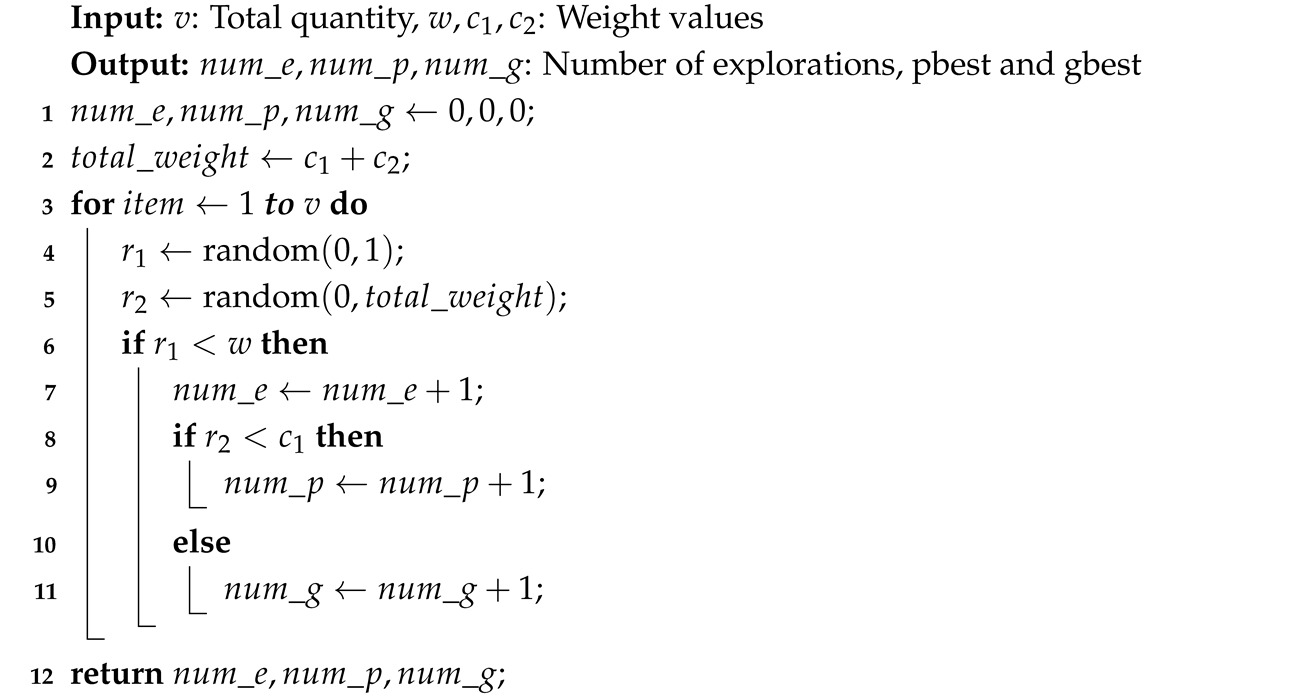
Algorithm 1: Update velocity.

Input: Current velocity v; weight w; cognitive coefficient $c_1$; social coefficient $c_2$; Current solution $current$; personal best $pbest$; global best $gbest$ Output: Updated velocity $v^{\prime }$ 1  $v^{\prime }\leftarrow v\times w$ 2  $ran{d}_1\leftarrow$ random number between 0 and 1 3  $ran{d}_2\leftarrow$ random number between 0 and 1 4  $j_1\leftarrow$ Jaccard distance between $current$ and $pbest$ 5  $j_2\leftarrow$ Jaccard distance between $current$ and $gbest$ 6  $v^{\prime }\leftarrow v^{\prime }+ran{d}_1\times c_1\times j_1+ran{d}_2\times c_2\times j_2$ 7  return $v^{\prime }$

4.2.3. Position Update Mechanism

To align with the modified velocity, we redefine position updates. Here, velocity $v_i$ represents the number of dimensions that will be modified in an update rather than a conventional movement vector. It is decomposed into three integer components: random exploration, movement toward personal best, and movement toward global best. The allocation is determined via roulette-wheel selection [48]. Figure 5 illustrates the position update process. In this example, the particle’s velocity is 5, meaning five dimensions in the list will be modified. During the five roulette-wheel selection steps, two dimensions undergo random exploration (blue region). The remaining three dimensions do not pass the first selection round, where one dimension moves toward the personal best (purple region) and two dimensions move toward the global best (orange region). Next, five dimensions in the list are randomly chosen for modification, with values replaced according to their assigned target category, ensuring that the new values are distinct from those already present in the list. The final outcome is an updated list (right side), completing one iteration of the position update process. This preserves diversity while ensuring targeted optimization.

4.2.4. Exploration Maintenance Mechanism

Elite evolution strategies significantly enhance the developmental capacity of algorithms while disrupting the balance between development and exploration, thereby reducing algorithmic diversity. To balance exploitation and exploration, we introduce a perturbation term c in the Jaccard distance:

$$D(A,B)=D_J(A,B)+c,$$

(17)

leading to the modified velocity update:

$$v_i^{t+1}=\omega ·v_i^t+c_1·r_1·D\left(X_{p,i}^t,X_i^t\right)+c_2·r_2·D\left(X_g^t,X_i^t\right),$$

(18)

This ensures dynamic adaptation, where early iterations favor exploration (higher velocity), while later iterations promote convergence (lower velocity) [49]. For details about the speed update process, see Algorithm 1. Additionally, in the position update mechanism, we modify the roulette selection to encourage random exploration. The $\omega$ value determines whether a particle should explore randomly, ensuring a high probability for random exploration. If random exploration does not occur, the individual best and global best particles compete for ownership via roulette selection. The algorithm pseudocode is detailed in Algorithm 2.

Algorithm 2: Roulette-wheel selection for position update.

Based on the roulette-wheel selection results, we randomly select $v_{i,j}$ dimensions and update them according to the assigned outcome. The selected dimensions undergo one of the following operations: random exploration, updating with a randomly chosen non-repeating item from the personal best solution, or swapping with a randomly chosen non-repeating item from the global best solution.

These improvements preserve population diversity and prevent premature convergence, enabling EEDPSO to efficiently explore the discrete solution space of RSs and provide high-quality recommendations with reduced computational overhead. The algorithm framework and process are detailed in Algorithm 3.

Algorithm 3: Elite evolutionary discrete particle swarm optimization.

Specifically, the pseudocode follows these steps: First, the swarm, global best solution, velocity, and other relevant parameters are initialized. In each iteration, the roulette-wheel selection mechanism is applied to update particle positions. Fitness values are then evaluated to determine whether to update particles, personal best solutions, and the global best solution. Subsequently, a small-scale neighborhood search is performed on the personal best and global best particles for further refinement. Finally, velocity and fitness history are updated. This process constitutes a single iteration, and, upon termination, the algorithm returns the fitness history and the global best solution.

The settings of $w=0.55$, $c_1$, and $c_2$ follow classical PSO guidelines [47], where moderate inertia and learning factors jointly ensure a balanced trade-off between exploration and exploitation. In our discrete RS scenario, we adopt a reduced total learning factor magnitude $c_1+c_2\approx 2.0$, deviating from the conventional value of $4.0$ in continuous PSO, to avoid excessive acceleration and instability. The perturbation term $c=2$ is introduced to dynamically enhance early-stage velocity and prevent premature convergence, especially in high-dimensional or noisy settings. The rationale and sensitivity of these parameter choices, including w, $c_1$, $c_2$, and the perturbation term c, are further examined in Section 6.2 and Section 6.3. These sections provide experimental evidence and comparative results that support the default values used in the EEDPSO framework.

The time complexity and the space complexity are

$$O(\mathrm{iterations}\times \mathrm{particles}\times [d+k\left]\right),$$

(19)

where iterations is the maximum number of iterations, particles is the number of particles, d is the length of the recommendation list, and k is the number of replacement items in the neighborhood search (determined by the velocity $v_v$).

$$O(\mathrm{particles}\times d),$$

(20)

which is used to store the positions of all particles and the optimal solutions.

5. Experiments and Analysis

In this section, we first describe our experimental setup, followed by a comparison of the results between the EEDPSO algorithm and other metaheuristic algorithms using curve plots, tables, and other visual representations.

Modern recommendation systems, especially in e-commerce, video recommendation, and digital advertising, often display content in a queue-like format, presenting the challenge of addressing the cold-start problem for new users with limited interaction history. EEDPSO is well suited to tackle this as its global search and local refinement capabilities effectively handle sparse data and adapt to the changing nature of user preferences. This makes EEDPSO particularly valuable in dynamic environments, where rapid shifts in user preferences demand accurate personalized recommendations. To evaluate EEDPSO’s performance in large-scale applications, we selected the MovieLens and Amazon datasets, which are widely used in movie recommendations and represent a variety of e-commerce products, respectively. We will validate the effectiveness of EEDPSO in real-world industrial applications for addressing cold-start situations and analyze its performance regarding these two public datasets.

Experimental Design. The experiment used four datasets, two of which are from popular public recommendation benchmarks: MovieLens-20m and MovieLens-32m. MovieLens-20m contains 20,000,263 ratings and 465,564 tag applications across 27,278 movies; MovieLens-32m includes 32,000,204 ratings and 2,000,072 tag applications across 87,585 movies [50,51]. The other two datasets come from the Amazon Review Data (2018), containing only rating data. They are named AmazonReviewData-sm, which includes AMAZON FASHION, Appliances, Prime Pantry, Software, All Beauty, and Magazine Subscriptions, with 283,931 products. AmazonReviewData-lg contains Books, Clothing Shoes and Jewelry, Cell Phones and Accessories, Automotive, CDs and Vinyl, Arts and Crafts, and Sewing, with 7,863,537 products [52]. Unlike the MovieLens datasets, AmazonReviewData consists of single-type products, and the average times of ratings per product are lower, requiring different adaptation criteria for fitness value calculation. All datasets were preprocessed into the format (index, item ID, item genres, average rating, and rating count) to suit the needs of non-personalized recommendation systems. The experiments were conducted on an i5 12,500 h 12-core CPU. To ensure randomization and reduce errors, the datasets were shuffled randomly for each experiment, and the average results of 100 trials were calculated. Hyperparameters were tuned based on analysis from the Optuna framework.

The datasets used in our experiments represent two major domains in recommendation systems: entertainment and e-commerce. MovieLens datasets (20 M and 32 M) are widely accepted public benchmarks for movie recommendation tasks, capturing typical user–item interaction behaviors in the context of digital media consumption. In contrast, the AmazonReviewData-sm and AmazonReviewData-lg datasets span a variety of product categories, from fashion and electronics to books and household items, thus reflecting diverse purchasing behaviors in a large-scale e-commerce setting. The contrast in rating sparsity, product diversity, and user engagement frequency between MovieLens and Amazon datasets provides a balanced testbed to evaluate the robustness of our algorithm across different data characteristics.

We compare the EEDPSO algorithm with five widely used metaheuristics: GAs, DE, SA, sine–cosine optimization (SCA), and PSO. GAs and SA are classical algorithms with strong industrial relevance, with GAs known for their global search capability [53] and SA effective for high-dimensional problems [54]. DE has demonstrated exceptional performance in algorithmic competitions and engineering optimization [55,56]. SCA, utilizing sine and cosine functions, achieves a balance between local exploitation and global exploration, offering high adaptability and stable performance across diverse optimization tasks without requiring complex hyperparameter tuning [57]. The following describes the configurations and operational principles of the algorithms in detail.

• Genetic algorithm (GA) evolves a population of candidate solutions through selection, crossover, and mutation. It employs tournament selection (size = 3) to choose parents, followed by two-point crossover, where a random segment is swapped between parents. Random replacement mutation is applied, replacing each gene with a new item with a small probability.
• Differential evolution (DE) generates new solutions through differential mutation, where a base solution is perturbed using the difference between two other randomly selected solutions. The resulting trial solution undergoes binomial crossover, where each gene is replaced with a probability $CR$. The better solution between the trial and original is selected for the next generation.
• Simulated annealing (SA) explores the solution space by applying random perturbations to the current solution. If the new solution improves fitness, it is accepted. Otherwise, it is accepted probabilistically based on the Boltzmann function $e^{\Delta f/T}$, allowing temporary acceptance of worse solutions to escape local optima. The temperature T decreases exponentially over iterations.
• Sine–cosine algorithm (SCA) updates solutions using a balance of exploitation (moving towards the best solution) and exploration (searching new areas). The update mechanism is guided by sine and cosine functions, ensuring smooth transitions between local and global search. Position correction mechanisms maintain valid solutions.
• Particle swarm optimization (PSO) models candidate solutions as particles that update positions based on velocity, which is influenced by inertia, personal best, and global best components. The updated position ensures uniqueness by removing duplicates.

To ensure fairness in the experiment, we implement the following measures: (1) standardizing algorithm applicability, balancing exploration, and equally allocating computational resources. For instance, we increase the number of iterations for simulated annealing (SA), a single-agent optimization algorithm, to match the computational scale of other algorithms by setting its iteration count to the product of population size and iterations [58]. (2) Minimizing random errors: Each experiment is repeated 100 times, and the average result is computed after excluding an equal proportion of the highest and lowest values. The random seed for each run is set as seed (42 + n), with 100 randomly generated tag heat lists assigned to each iteration. (3) Efficient resource utilization: We optimize hyperparameters using the Optuna framework, employing Bayesian optimization and pruning to intelligently explore the parameter space [59]. The EEDPSO slice plot in Figure 6 highlights regions of high search density, indicating promising hyperparameter combinations, while darker points suggest optimal regions. This approach validates the effectiveness of the optimization framework, with the most effective hyperparameters presented in the next section.

We additionally compare EEDPSO with two representative deep learning models: FairGo and the PRM. FairGo is a graph-based model designed to ensure fairness in recommendation, while the PRM (personalized re-ranking model) enhances list quality via transformer-based re-ranking. These models represent state-of-the-art approaches in fairness-aware and personalized recommendation. In the experiment, we used the default settings in the model open-source code and only deleted the user portrait and personalization parts. In addition, due to the different resource usage of model training, we gave the model a lower number of iterations.

6.

FairGo (fair-graph-based recommendation) mitigates recommendation bias by learning fair user/item embeddings. It applies adversarial training to remove sensitive attribute signals (e.g., gender or age) from both user embeddings and their ego-centric graph structures. This ensures the recommendation process is fair while maintaining accuracy.

7.

The PRM (personalized re-ranking model) refines initial recommendation lists using a transformer-based encoder with user-specific embeddings. By modeling mutual item interactions and user intent via self-attention, the PRM reorders the list to better match user preferences. It operates efficiently and supports large-scale deployment in real-time systems.

To ensure a fair and controlled comparison, we remove user profile and personalized embedding components from the original open-source implementations of both models while preserving all other architectural modules. This modification allows us to isolate the effect of their core re-ranking mechanisms in a non-personalized recommendation setting, aligning with the evaluation scope of EEDPSO. All experiments are independently run 100 times, and the average results are compiled. The hyperparameters used are the recommended settings from the study to ensure the model’s performance is properly reflected.

Comparison Criteria. To compare the performance of different algorithms, we evaluate and record the final fitness, worst fitness, fitness standard deviation, termination generation, and runtime. A Wilcoxon rank-sum test is conducted to assess the statistical significance of differences in final fitness, providing a comprehensive evaluation of algorithmic performance. The test results are presented in a comparative table. Additionally, we visualize the experimental results using four types of plots: average fitness curve, box plot, fitness distribution plot, and scatter plot. These charts provide insights into convergence trends, final statistics, distribution characteristics, and single-run dispersion. The comparison criteria are as follows:

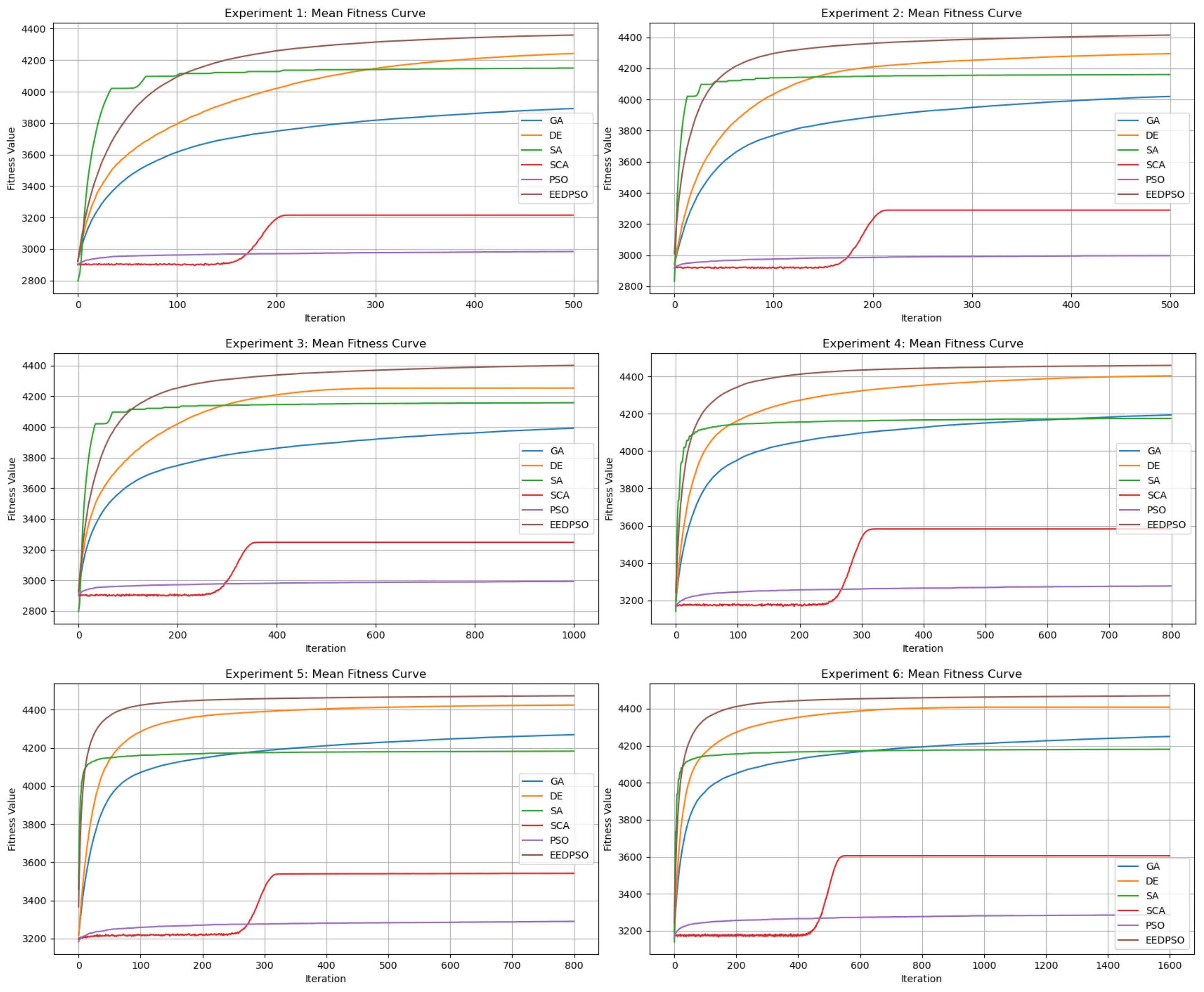
• Average Fitness Curve: This plot shows the evolution of the algorithm’s average fitness over time or generations, illustrating its convergence speed and improvement during later stages.
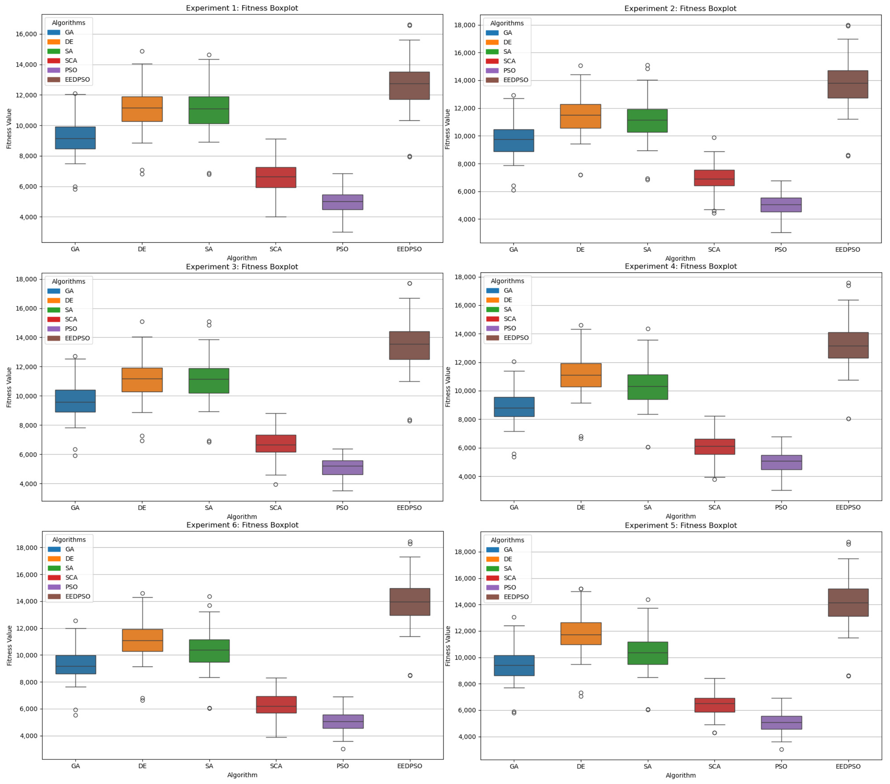
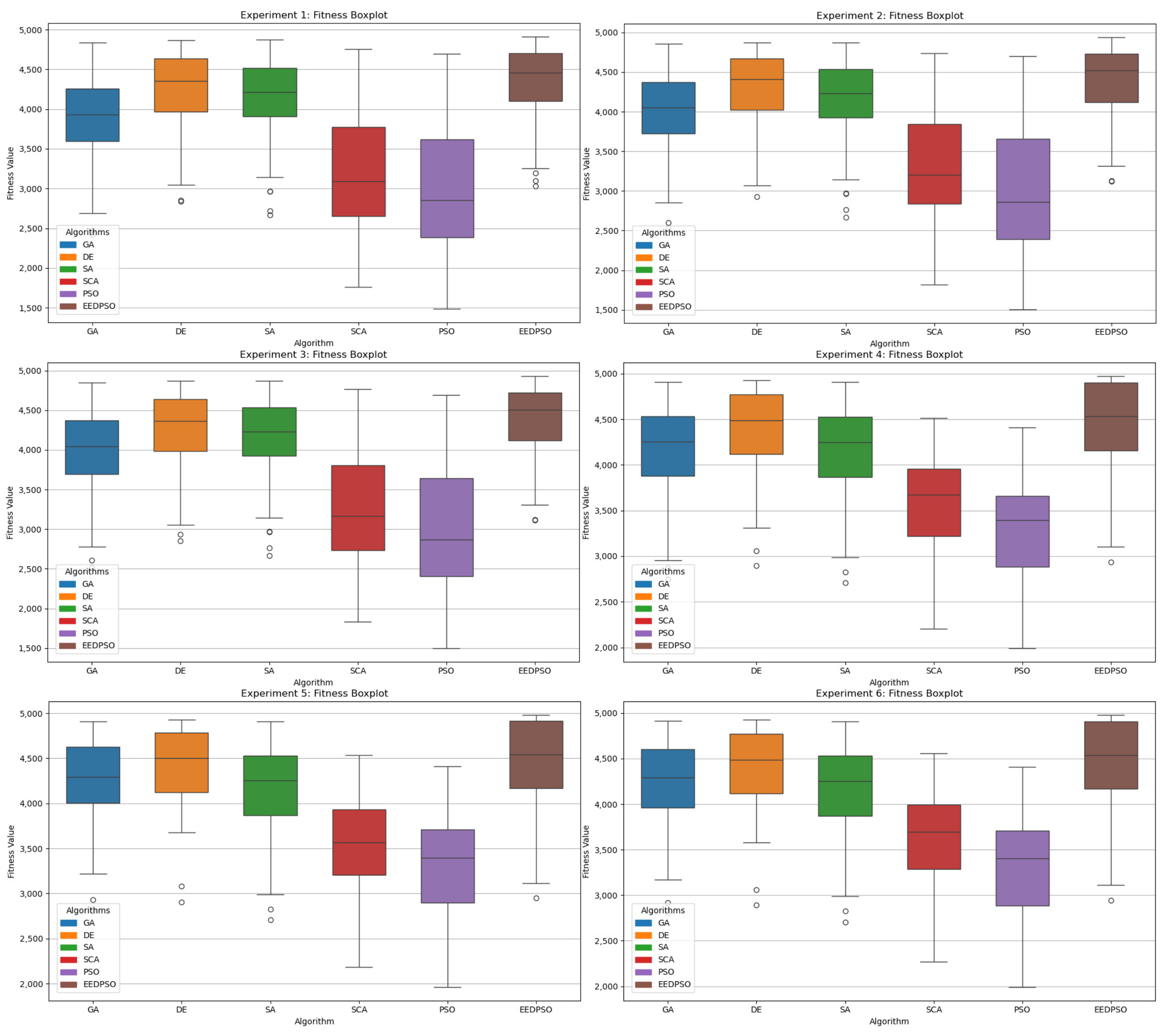
• Box Plot: The box plot displays the median, quartiles, and outliers of the final fitness distribution, reflecting the algorithm’s robustness across multiple runs and highlighting the best and worst solutions.
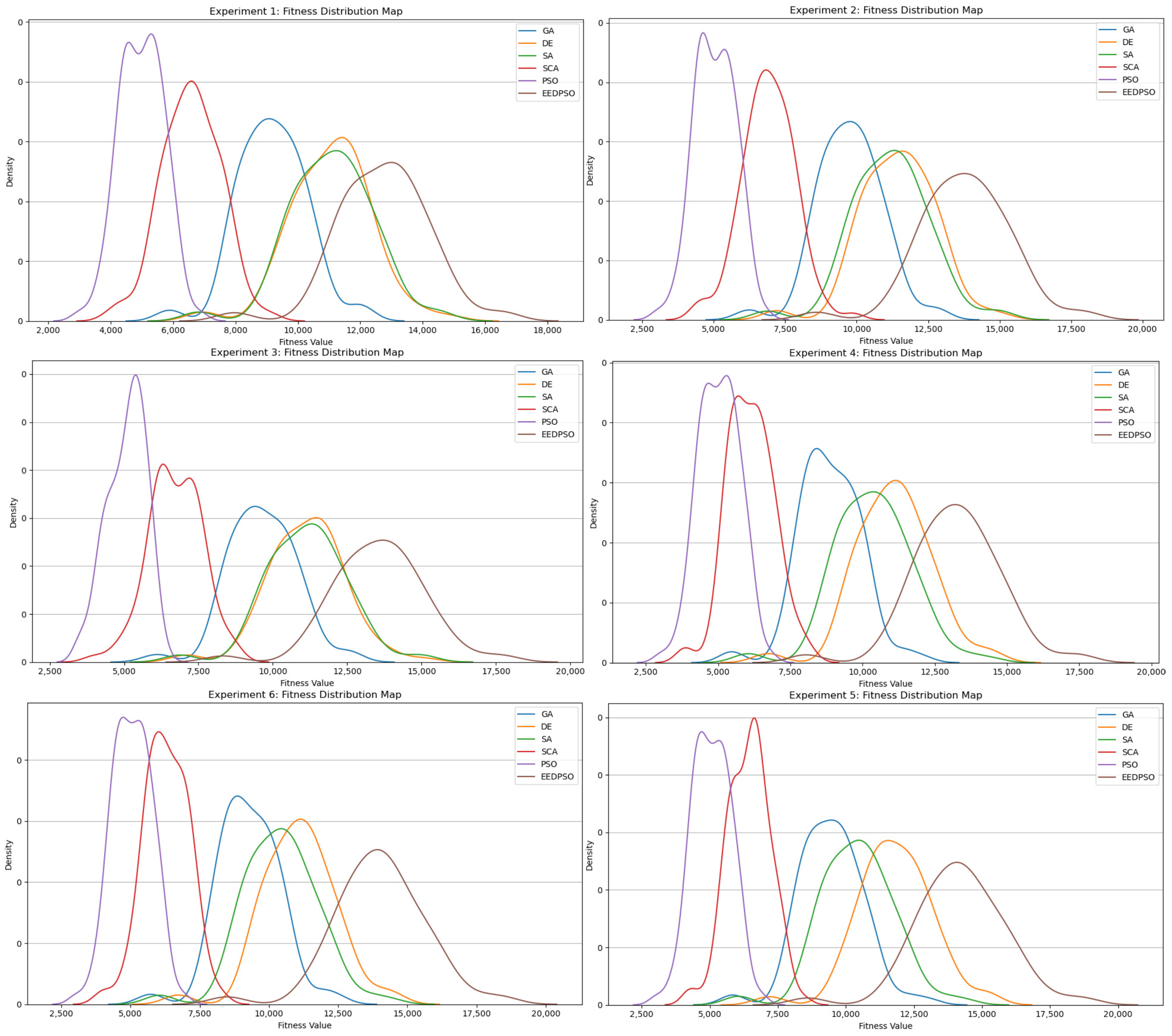
• Fitness Distribution Plot: Using kernel density estimation or smoothed histograms, this plot presents the probability distribution of final fitness values from multiple trials, revealing the concentration and tail behavior of the algorithm’s solutions.
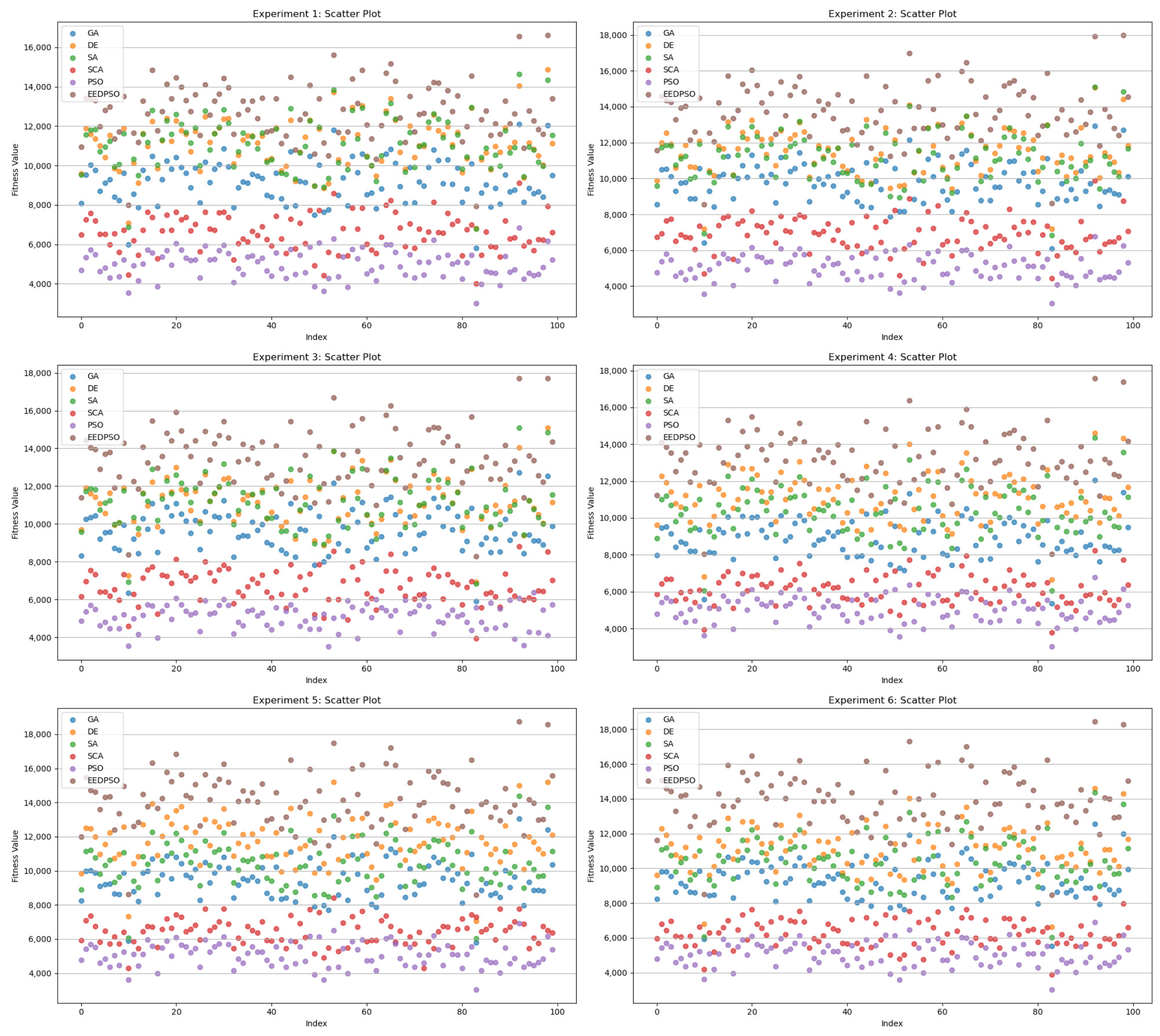
• Scatter Plot: This plot sets the trial index on the horizontal axis and the final fitness value on the vertical axis, allowing for assessment of solution quality and consistency across independent runs.

Number of Iterations and Number of Particles. In practical applications, the number of particles and iterations in EEDPSO can be adjusted according to the problem scale. For low-dimensional or small-to-medium recommendation tasks, we recommend setting the particle number to 30–50 and the number of iterations to 200–500 to ensure both efficiency and solution quality. In high-dimensional or large-scale scenarios, increasing the particle count to 75–150 and iterations to 800–1600 can improve search robustness and convergence quality. These ranges are derived from our experimental experience and can be further optimized using hyperparameter search frameworks such as Optuna. In scenarios where computational speed is critical—such as real-time recommendations or edge device deployment—a trade-off must occur between performance and efficiency. In such cases, a reduced number of particles and iterations may be used to limit computational cost, although this may slightly compromise optimization depth. The specific trade-offs can be guided by our experimental results presented in the following sections.

Hyperparameter Experiments. We conduct hyperparameter optimization using the Optuna framework, performing 100 trials. The best-performing hyperparameter combination is selected, with Bayesian optimization and pruning strategies progressively refining the sampling process to converge towards the global optimum. The final results are presented in

Table 2. Hyperparameter search experiment.

	MovieLens-20m		MovieLens-32m		AmazonReviewData-sm		AmazonReviewData-lg
GA	cxpb	0.58	cxpb	0.73	cxpb	0.94	cxpb	0.79
	mutpb	0.16	mutpb	0.13	mutpb	0.2	mutpb	0.2
DE	F	0.3	F	0.33	F	0.37	F	0.27
	CR	0.84	CR	0.69	CR	0.71	CR	0.92
SA	initial_temperature	258.77	initial_temperature	124.23	initial_temperature	133.86	initial_temperature	207.62
	cooling_rate	0.99	cooling_rate	0.87	cooling_rate	0.99	cooling_rate	0.95
	alpha	0.84	alpha	0.94	alpha	0.89	alpha	0.90
	perturbation_size	1.00	perturbation_size	1.00	perturbation_size	1.00	perturbation_size	1.00
PSO	w	0.53	w	1.03	w	0.8	w	1.17
	c1	1.67	c1	1.40	c1	2.12	c1	1.98
	c2	1.19	c2	1.16	c2	2.12	c2	1.27
EEDPSO	w	0.55	w	0.67	w	0.52	w	0.69
	c1	1.26	c1	1.23	c1	1.13	c1	1.11
	c2	0.74	c2	0.64	c2	0.91	c2	0.89

. In the subsequent comparative experiments, the chosen hyperparameters are applied according to the dataset size.

Design of Comparison. We conducted twelve experimental setups using MovieLens-20m, MovieLens-32m, AmazonReviewData-sm, and AmazonReviewData-lg. For the purpose of differentiation, the experiments were designated as Experiment 1 through Experiment 12, each generating a recommendation list of 200 items, resulting in 8 control experiments, as shown in

Table 3. Experiments on different sizes of MovieLens-20M.

			Fitness	Worst Fitness	Standard Deviation	Convergence Generation	p-Value	Significant	Time (s)
Experiment 1	GA	ngen = 500 pop = 80 particles = 30	9184.99	5431.11	809.34	481	0	****	17.93
	DE		11,068.45	5439.99	1180.69	472	$1.8596\times {10}^{-15}$	****	16.04
	SA		11,079.88	5047.36	798.39	305	$6.407\times {10}^{-15}$	****	4.33
	SCA		6584.37	5183.51	555.91	202	0	****	32.58
	PSO		4989.12	4670.35	51.07	246	0	****	7.57
	EEDPSO		12,741.04	5496.08	1450.12	496	*	*	7.9
Experiment 2	GA	ngen = 500 pop = 200 particles = 75	9766.18	5463.31	873.35	481	0	****	44.37
	DE		11,452.14	5501.96	1164.35	486	0	****	53.81
	SA		11,175.88	5257.64	525.21	294	0	****	10.2
	SCA		6915.61	5266.28	688.09	207	0	****	79.95
	PSO		5042.56	4733.8	51.08	216	$0.00$	****	19.13
	EEDPSO		13,777.85	5816.11	1360.3	497	*	*	18.6
Experiment 3	GA	ngen = 1000 pop = 80 particles = 30	9652.39	5431.11	781.65	960	0	****	35.24
	DE		11,141.38	5439.99	1098.75	497	0	****	25.62
	SA		11,145.64	5047.36	599.52	558	0	****	8.14
	SCA		6716.21	5175.46	597.81	346	0	****	62.88
	PSO		5086.81	4739.93	48.69	516	0	****	15.39
	EEDPSO		13,542.45	5478.1	1407.47	993	*	*	14.97
DRS Experiment 1	FairGo	ngen = 200	11,076.8	3931.66	1295.16	197
	PRM		4722.95	4304.71	132.26	82 (early stopping)

The bolded values represent the relatively optimal data, with the p-value significance indicated as follows: *: p-value < 0.05, ****: p-value < 0.0001.

,

Table 4. Experiments on different sizes of MovieLens-32M.

			Fitness	Worst Fitness	Standard Deviation	Convergence Generation	p-Value	Significant	Time (s)
Experiment 4	GA	ngen = 800 pop = 120 particles = 45	8872.67	4780.43	739.47	764	0	****	43.52
	DE		11,088.85	4792.31	1253.44	591	$2\times {10}^{-20}$	****	35.22
	SA		10,359.6	4975.74	538.38	461	0	****	9.92
	SCA		6123.51	4549.07	636.21	298	0	****	77.21
	PSO		5022.42	4696.83	46.72	404	0	****	24.64
	EEDPSO		13,241	4903.1	1453.34	795			18.92
Experiment 5	GA	ngen = 800 pop = 300 particles = 110	9458.04	4848.85	776.01	768	0	****	110.37
	DE		11,792.77	4855.48	1216.69	786	0	****	125.27
	SA		10,426.62	5770.2	354.33	403	0	****	25.27
	SCA		6436.12	4689.2	728.37	304	0	****	196.82
	PSO		5067.66	4764.2	42.5	428	0.00	****	60.96
	EEDPSO		14,209.51	5341.78	1333.98	795	*	*	46.12
Experiment 6	GA	ngen = 1600 pop = 120 particles = 45	9278.33	4780.43	691.79	1550	0	****	90.61
	DE		11,089.61	4792.31	1042.8	592	0	****	59.08
	SA		10,415.96	4975.74	406.81	847	0	****	20.43
	SCA		6285.38	4541.12	690.43	521	0	****	151.66
	PSO		5054.24	4696.83	44.51	831	0	****	50.47
	EEDPSO		14,007.29	4917.78	1374.89	1591	$1\times {10}^{-4}$	*	37.93
DRS Experiment 2	FairGo	ngen = 320	12,188.82	3546.43	1474.85	315
	PRM		4642.94	4256.76	182.54	117 (early stopping)

The bolded values represent the relatively optimal data, with the p-value significance indicated as follows: *: p-value < 0.05, ****: p-value < 0.0001.

,

Table 5. Experiments on different sizes of AmazonReviewData-sm.

			Fitness	Worst Fitness	Standard Deviation	Convergence Generation	p-Value	Significant	Time (s)
Experiment 7	GA	ngen = 500 pop = 80 particles = 30	3892.64	2920.16	190.08	483	$2.616\times {10}^{-11}$	****	18.77
	DE		4242.21	2923.55	272.28	466	0.0181852	*	13.54
	SA		4149.65	4975.74	173.52	292	$6.4068\times {10}^{-15}$	****	4.63
	SCA		3215.52	2849.87	145.3	209	0	****	36.37
	PSO		2984.39	2899.95	13.17	255	0	****	8.84
	EEDPSO		4359.57	2924.65	266.02	496	*	*	7.98
Experiment 8	GA	ngen = 500 pop = 200 particles = 75	4019.59	2939.12	200.15	487	$1.1656\times {10}^{-9}$	****	47.2
	DE		4294.45	2940.93	256	485	0.0097806	**	48.64
	SA		4160.08	2833.14	109.67	264	$2.9328\times {10}^{-5}$	****	11.53
	SCA		3288.77	2871.74	172.92	214	0	****	82.54
	PSO		2996.51	2916.77	13.74	242	0.00	****	21.78
	EEDPSO		4414.12	3009.19	191.6	496	*	*	19.48
Experiment 9	GA	ngen = 1000 pop = 80 particles = 30	3992.14	2920.16	177.98	969	$6.2754\times {10}^{-10}$	****	37.42
	DE		4253.65	2923.55	232.91	488	0.00316204	*	19.96
	SA		4157.76	2796.79	127	530	$6.6\times {10}^{-5}$	****	9.23
	SCA		3247.24	2847.69	155.14	355	0	****	69.45
	PSO		2992.83	2899.95	13.11	488	0	****	19.46
	EEDPSO		4401.49	2929.27	212.26	994	*	*	15.83
DRS Experiment 3	FairGo	ngen = 200	4319.91	1432.51	733.94	192
	PRM		2287.48	2175.73	24.65	79 (early stopping)

The bolded values represent the relatively optimal data, with the p-value significance indicated as follows: *: p-value < 0.05, **: p-value < 0.01, ****: p-value < 0.0001.

and

Table 6. Experiments on different sizes of AmazonReviewData-lg.

			Fitness	Worst Fitness	Standard Deviation	Convergence Generation	p-Value	Significant	time(s)
Experiment 10	GA	ngen = 800 pop = 120 particles = 45	4193.66	3194.59	153.88	783	$4.1371\times {10}^{-6}$	****	39.25
	DE		4403.42	3197.31	174.41	684	0.0369414	*	27.82
	SA		4174.95	3140.4	65.24	417	$2.9657\times {10}^{-6}$	****	9.81
	SCA		3582.69	3112.19	189.58	315	0	****	72.9
	PSO		3277.02	3164.8	16.4	401	0	****	27.76
	EEDPSO		4459.33	3241.8	134.69	794	*	*	24.59
Experiment 11	GA	ngen = 800 pop = 300 particles = 110	4269.09	3214.48	150.43	785	0.00010553	**	98.4
	DE		4424.1	3216.91	160.26	782	0.0315705	*	97.09
	SA		4182.63	3457.91	37.3	407	$2.0186\times {10}^{-6}$	****	24.42
	SCA		3541.79	3161.69	151.13	341	0	****	188.81
	PSO		3290.26	3183.18	16.06	404	0.00	****	58.73
	EEDPSO		4472.8	3366.29	89.53	795	*	*	45.64
Experiment 12	GA	ngen = 1600 pop = 120 particles = 45	4249.83	3194.59	132.54	1569	$5.4618\times {10}^{-5}$	****	78.34
	DE		4408.43	3197.31	136.56	699	0.0310538	*	40.76
	SA		4181.02	3140.4	47.84	864	$2.1407\times {10}^{-6}$	****	19.45
	SCA		3605.47	3109.71	194.08	546	0	****	143.75
	PSO		3286.44	3164.8	15.96	805	0	****	46.01
	EEDPSO		4470.09	3242.12	100.91	1591	*	*	34.3
DRS Experiment 3	FairGo	ngen = 320	4650.32	1416.29	816.2	316
	PRM		2445.43	2198.55	37.05	87 (early stopping)

The bolded values represent the relatively optimal data, with the p-value significance indicated as follows: *: p-value < 0.05, **: p-value < 0.01, ****: p-value < 0.0001.

. Experiments (1, 2), (4, 5), (7, 8), (10, 11) serve as scale comparison experiments, while Experiments (1, 3), (4, 6), (7, 9), (10, 12) serve as iteration count comparison experiments. As shown in Figure 7, Figure 8, Figure 9, Figure 10, Figure 11, Figure 12, Figure 13 and Figure 14, the data from the tables and figures allow for the analysis of general trends. To further compare EEDPSO with deep-learning-based re-ranking methods, we conducted additional experiments using FairGo and the PRM. These deep recommendation system (DRS) experiments are labeled as DRS Experiment 1 through DRS Experiment 4, corresponding to the four datasets. The results are presented alongside the metaheuristic comparisons in the same set of tables for clarity.

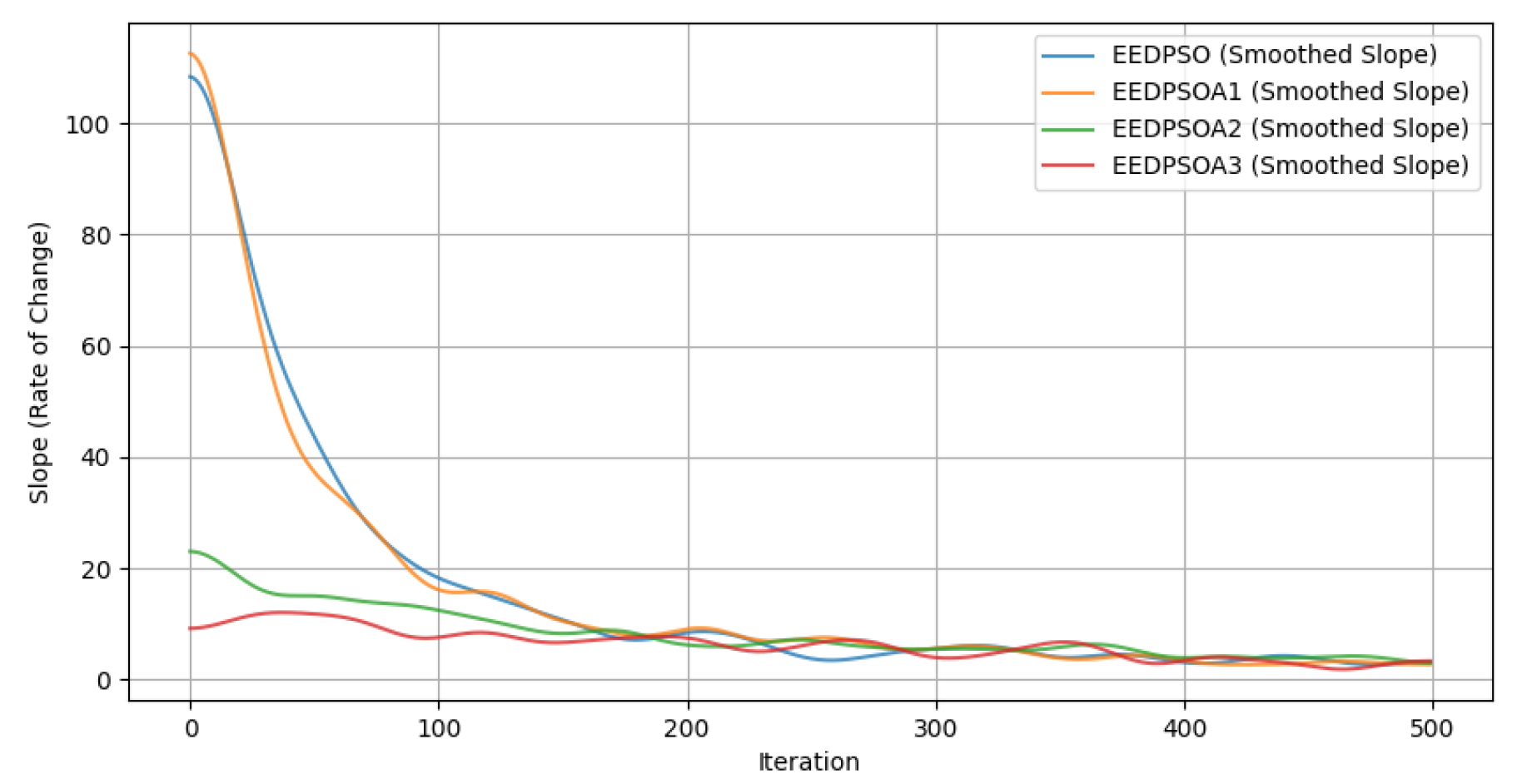
• The EEDPSO curve in the fitness graph is the highest and shows significant improvement in later stages, demonstrating strong global search and local fine-tuning capabilities. As iterations progress, its late-stage advantages become more evident. DE and SA perform at a mid-to-high level, with SA excelling in early-stage speed. GAs show moderate performance but exhibit continuous growth.
• In the box plot, EEDPSO has the highest median and maximum values, indicating stable solution quality and occasional optimal solutions. DE and SA rank second, with DE slightly outperforming SA in extreme values. GAs show substantial fluctuations but generally remain moderate.
• In the distribution plot, the EEDPSO curve is right-shifted and has the longest tail, indicating superior initial performance and optimization ability. Its low peak suggests the algorithm avoids stagnation in specific regions, showcasing strong exploration. EEDPSO offers higher solution diversity and a broader search range than other algorithms.
• In the scatter plot, EEDPSO achieves the highest mean and a broad distribution range, indicating consistent convergence to high-quality solutions rather than occasional outliers.

Based on the comprehensive analysis of the visualization results, we can conclude that EEDPSO demonstrates both fast and stable convergence across diverse experimental conditions. As shown by the convergence curves and convergence generation metrics, it achieves rapid fitness improvements during the early iterations and continues to refine solutions in the later stages. In contrast, algorithms such as SA and DE converge quickly at first but tend to plateau early, resulting in lower final fitness. This reflects EEDPSO’s ability to maintain a balanced search process that combines global exploration with effective local refinement.

In large-scale and high-dimensional scenarios—such as MovieLens-32M and AmazonReviewData-lg—EEDPSO maintains strong robustness and avoids premature convergence. Its discrete position update strategy, adaptive perturbation mechanism, and diversity-preserving components allow it to sustain effective search dynamics as problem complexity increases. These convergence characteristics are especially beneficial in real-world recommendation tasks, which are typically sparse, dynamic, and combinatorial in nature.

Firstly, we analyze the experiments of the metaheuristic algorithms. The fitness performance analysis across twelve experimental groups reveals consistent rankings among the algorithms. EEDPSO consistently achieves the highest or near-highest fitness values, demonstrating superior global search capability and local refinement efficiency. Worst-case fitness analysis indicates that EEDPSO performs well in the early stages. Statistical significance analysis, including p-values, confirms that EEDPSO significantly outperforms other algorithms. DE and SA form the second tier, exhibiting comparable performance, with variations dependent on parameter settings and experimental conditions. While SA converges rapidly, its final fitness values are generally similar to or slightly lower than those of DE. GAs perform at an intermediate level, outperforming SCA and PSO, both of which struggle with the recommendation optimization task.

When computational scale (population size and particles) increases, GAs and DE show notable improvements due to particle interactions. As the iteration count increases, DE and SA reach full convergence, and their fitness values stabilize. EEDPSO maintains its advantage throughout.

EEDPSO and GAs take the longest to converge, suggesting slower convergence in standard optimization problems [20]. However, in a 200-dimensional combinatorial optimization problem, this highlights their superior exploration capabilities. DE also improves exploration when the computational scale is sufficiently large.

Regarding computation time, SA has the shortest runtime, outperforming GAs, DE, and SCA. EEDPSO follows with overall efficient computation. DE and GAs, with their large populations and complex operations, experience a superlinear increase in computation time as the computational scale grows. SCA is unsuitable for high-dimensional problems. As particle numbers and iterations increase, EEDPSO’s computational speed advantage over PSO becomes more pronounced, indicating that modifications to velocity and position updates enhance its adaptability and efficiency in this experimental setup.

We then conducted a comparative analysis of the EEDPSO experiment with two deep recommendation systems. In the cold-start recommendation scenarios across the first three datasets, EEDPSO demonstrates clear advantages in recommendation precision. Its robustness in sparse environments enables it to consistently outperform the deep learning models under limited interaction data. FairGo, a graph-based model designed to enhance fairness, shows competitive performance and better scalability as data volume increases. Specifically, on the largest dataset (AmazonReviewData-lg), FairGo slightly surpasses EEDPSO in recommendation accuracy due to its graph convolution structure’s effectiveness in large-scale user–item relationships.

The PRM, in contrast, is a transformer-based re-ranking model that relies heavily on the presence of rich user profiles to learn personalized embeddings. While the PRM performs well in scenarios with extensive user interaction histories and complete side information, it is not well suited for cold-start settings. Its re-ranking capacity assumes a meaningful initial list and personalized vector input, both of which are difficult to obtain in cold-start environments. This explains the PRM’s consistently low performance in our experiments, reaffirming its limitations under sparse-data conditions.

Conclusion. EEDPSO excels due to its balance of global search and local refinement, which is essential for high-dimensional, sparse, and combinatorial optimization problems such as recommendation systems. Unlike traditional PSO, which struggles in discrete spaces, EEDPSO modifies the velocity and position update mechanisms to suit discrete recommendation lists. Its neighborhood search enhances local exploitation, while the modified velocity update based on Jaccard similarity improves stability. The roulette-wheel selection for position updates maintains diversity and prevents premature convergence, ensuring effective exploration. Additionally, the perturbation term dynamically adjusts the balance between exploration and exploitation, preventing early stagnation and enhancing performance in noisy high-dimensional environments. These innovations enable EEDPSO to effectively address challenges like the cold-start problem in recommendation systems and maintain robust performance across different datasets and parameter settings.

The performance of other algorithms, such as GAs, DE, SA, PSO, and SCA, falls short for discrete and high-dimensional recommendation system problems due to their inherent limitations. GAs, while effective for global search, suffer from slow convergence and high computational cost, especially in large datasets. DE excels in global search but struggles with early-stage adaptation, often requiring more computational resources to refine solutions in sparse-data scenarios. SA, although fast in early convergence, is more prone to local optima and struggles with high-dimensional, sparse spaces, limiting its effectiveness in complex recommendation tasks. PSO tends to concentrate particles in certain regions, limiting its ability to explore the entire solution space, which hampers its performance in discrete and combinatorial optimization tasks. SCA, although effective in continuous optimization tasks, is not suitable for discrete problems like recommendation systems due to its reliance on sine and cosine functions, which do not align with the discrete nature of recommendation lists.

In addition to classical metaheuristic algorithms, we compared EEDPSO with two deep-learning-based re-ranking models: the PRM and FairGo. In cold-start scenarios across sub-million-scale datasets, EEDPSO significantly outperforms both deep models, owing to its ability to explore sparse spaces without relying on user profiles or pre-trained embeddings. FairGo, while designed primarily to improve fairness, leverages graph-based representation learning that offers partial robustness under data sparsity. As a result, on the largest dataset (AmazonReviewData-lg), FairGo achieves slightly higher accuracy than EEDPSO, benefiting from its structural modeling of user–item relations. The PRM, in contrast, consistently underperforms in cold-start environments due to its reliance on rich user interaction histories and personalized embeddings, which are unavailable in sparse settings.

Overall, EEDPSO is the optimal choice for enhancing satisfaction or revenue optimization in complex recommendation system tasks, especially under data sparsity or cold-start conditions. Across twelve experiments, it consistently outperforms traditional metaheuristics and maintains competitive performance against advanced deep models, demonstrating superior efficiency, robustness in discrete recommendation optimization, and strong generalizability and reliability.

6. Discussion

In this section, we conduct an ablation study using the first experimental group from Section 5, where the iteration count is 500, the particle count is 30, and all the hyperparameters remain consistent. To ensure fairness and minimize random errors, we use the same seed and tag heat parameters in each experiment and take the average results over 100 runs. This study further analyzes and answers the following questions:

• The elite evolution strategy consists of two modules. How does each module contribute to improving algorithm performance?
• The experimental results indicate that the new velocity update strategy performs well in solving optimization problems. How is its effectiveness reflected in the results?
• The new position update strategy guides particles toward more targeted random exploration. What are its actual effects?
• Under the combined influence of multiple strategies, how should parameters $c_1$ and $c_2$ be proportionally allocated in EEDPSO? Does this allocation help to balance exploration and exploitation?

In the following sections, we provide answers to these questions.

6.1. Elite Evolution Strategy

The elite evolution strategy in the algorithm is implemented through neighborhood exploration of both the personal best and global best solutions. To evaluate its effectiveness, we conduct ablation experiments by sequentially removing each component. The experimental setup is as follows: Experiment 1 (EEDPSO): the complete algorithm. Experiment 2 (EEDPSOA1): personal best neighborhood exploration removed. Experiment 3 (EEDPSOA2): global best neighborhood exploration removed. Experiment 4 (EEDPSOA3): both neighborhood exploration strategies removed.

According to

Table 7. Ablation study results and relative performance changes.

Experiment	Fitness	Time (s)	Fitness Change (%)	Time Change (%)
EEDPSO	13,394.04	7.94	0.00	0.00
EEDPSOA1	12,608.43	5.86	−5.72	−26.26
EEDPSOA2	8953.20	6.00	−33.17	−24.56
EEDPSOA3	8150.71	4.32	−39.17	−45.60

, global best neighborhood exploration significantly improves computational quality. From the fitness curve in Figure 15, both strategies exhibit strong global search capabilities and contribute to mitigating premature convergence. To better understand their respective roles, we analyze the slope (derivative) curve. The obtained slope data are smoothed using Gaussian filtering to reduce noise, allowing for a clearer visualization of key trends [60]. From the Figure 16 slope curve, it is evident that the impact of both strategies on the growth rate is primarily in the early iterations, with global best neighborhood exploration being significantly more influential. These findings indicate that global best neighborhood exploration serves as a fundamental component in EEDPSO, while personal best neighborhood exploration contributes an additional 6–10% improvement in computational quality. The synergistic interaction between these two strategies is the key factor behind EEDPSO’s superior performance.

Second, we conduct an analysis of the relative importance and interaction effects of the two key components in the proposed algorithm: the personal-best neighborhood exploration strategy (personal) and the global-best neighborhood exploration strategy (global). As shown in Figure 17, we analyze the four subplots in order from left to right, top to bottom.

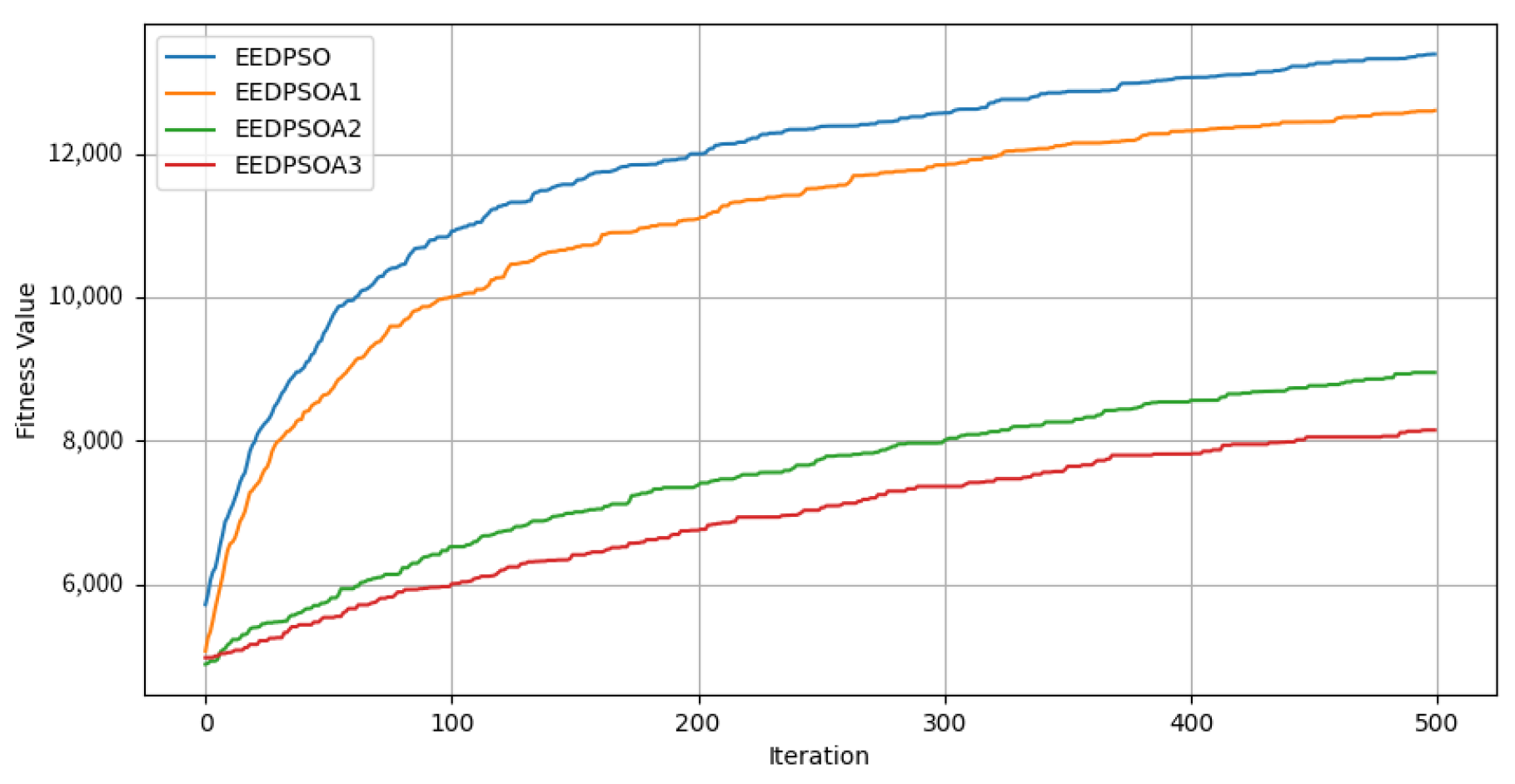
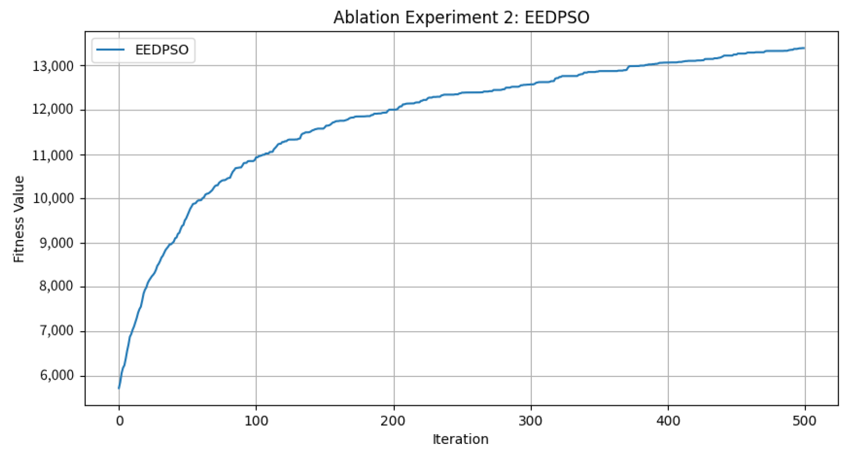
• Final Fitness Distribution (a). This subplot illustrates the final fitness distributions of the four experimental variants: the full algorithm (EEDPSO) and three ablation versions (EEDPSOA1, EEDPSOA2, and EEDPSOA3). The full algorithm achieves the highest performance overall, with a clearly higher median and upper quartile. In contrast, EEDPSOA3—which removes both components—demonstrates a significant drop in performance, as indicated by the leftward shift in distribution. This result suggests that the absence of both strategies substantially impairs the algorithm’s global search ability and convergence effectiveness.
• Performance Scatter Comparison (b). This subplot compares the final fitness results of each ablated version with those of the full algorithm. The dense and separated clusters, especially for EEDPSOA3, reveal that jointly removing both personal and global components significantly degrades performance. The other two ablation variants show milder performance degradation, indicating that either component alone contributes positively to optimization, but the joint presence is crucial.
• Interaction Effect Analysis (c). This subplot presents the interaction effect between the two components, visualized through a point plot derived from a linear regression model with an interaction term (Fitness Personal + Global + Personal × Global). The two lines (Global = 0 and Global = 1) are clearly non-parallel and intersect, indicating the presence of an interaction effect. Although the interaction term is not statistically significant (p = 0.176), the trend suggests that the combined removal of both components causes a synergistic deterioration in fitness, beyond the sum of their individual effects.
• Correlation Matrix of Experimental Results (d). The final subplot shows the Pearson correlation matrix among the four experiment groups. EEDPSO and EEDPSOA1 exhibit the highest correlation (r = 0.99), suggesting that removing only the personal component does not substantially change the search behavior. On the other hand, EEDPSOA3 shows the lowest correlation with the full algorithm (r = 0.96), implying that removing both components significantly alters not just the performance but the behavior and search dynamics of the algorithm.

6.2. Changes in Update Mechanisms

We address Question 2 and Question 3 simultaneously by analyzing both the velocity update mechanism and the position update mechanism.

The velocity update mechanism primarily incorporates Jaccard distance with an added perturbation term c to measure particle distance while retaining the standard PSO update rule. In discrete recommendation lists, Jaccard similarity proves especially suitable as it measures the set similarity between recommendation lists, providing an intuitive metric for discrete recommendation systems [61]. Jaccard similarity offers several advantages for our approach: it has low computational complexity, maintains a bounded value range of [0,1] that aligns with PSO requirements, accurately reflects structural similarities between recommendation lists, and effectively handles sparse high-dimensional data. Alternative metrics show notable limitations: cosine similarity better suits continuous vector spaces compared to discrete structures; Pearson correlation coefficients struggle to represent structural differences between recommendation lists; and Euclidean distance incurs high computational costs in high-dimensional spaces while producing unbounded values that complicate velocity control [61]. For the perturbation value c, optimization using the Optuna framework identifies an optimal range of 2–4, within which particle velocity gradually decreases to promote convergence while maintaining sufficient exploratory capability to avoid local optima. The perturbation term c plays a critical role in enhancing exploration in PSO, particularly in discrete recommendation scenarios. In standard PSO, particle velocities tend to shrink near optimal regions, increasing the risk of premature convergence. By introducing a controlled random perturbation, c disrupts this equilibrium, enabling particles to escape local traps and continue global exploration. Moreover, in conjunction with guidance from the center-nearest particle (CNP), the perturbation term increases population diversity and reduces the likelihood of particles clustering prematurely. This mechanism effectively strengthens the algorithm’s global search ability and robustness, ensuring stable convergence and improved adaptability in complex high-dimensional search spaces [62].

As shown in Figure 18, the lowest peak values of velocity in EEDPSO exhibit a decreasing trend over iterations during the jumping process. This aligns with our intended effect, where the inertia weight ($\omega$) effectively regulates velocity throughout optimization. As the algorithm progresses, the particles’ reliance on their current velocity diminishes, leading to a continuous reduction in the lower bound of velocity.

Position Update Mechanism: We employ a roulette-wheel selection strategy for position updates, balancing random exploration, personal best ($pbest$) exploitation, and global best ($gbest$) optimization. The inertia weight ($\omega$) governs the extent of random exploration and should be set inversely proportional to the perturbation in the distance function to maintain equilibrium between velocity fluctuations and decay (as analyzed in Section 4). An appropriate range for $\omega$ is 0.5 to 0.65, ensuring that approximately half of the dimensions undergo random exploration. Excessively high $\omega$ values may hinder convergence, undermining the intended PSO behavior.

The modifications to the velocity and position update mechanisms preserve the simplicity of the PSO update process, requiring only a single update per iteration. This effectively reduces the computational cost while maintaining the algorithm’s exploratory capacity. The velocity update mechanism ensures a gradual decrease in velocity while allowing significant jumps, enabling broader participation of dimensions in the update process. Simultaneously, the position update mechanism ensures sufficient dimensional perturbation, facilitating continuous global exploration as the algorithm converges. This enhances the ability to escape local optima and improves the global search efficiency.

Comparing the EEDPSO and EEDPSOA3 curves in Figure 19 and Figure 20, we observe that, without neighborhood exploration, the growth curve exhibits a step-like pattern. This suggests that the algorithm struggles to efficiently exploit local regions, instead favoring broader exploration to escape local optima and enhance the global search. At this stage, increased randomness mitigates premature convergence.

In metaheuristic algorithms, a step-like growth pattern is generally indicative of suboptimal performance [53]. However, in this case, it complements the elite evolution neighborhood exploration strategy, achieving a dynamic balance between exploration and exploitation.

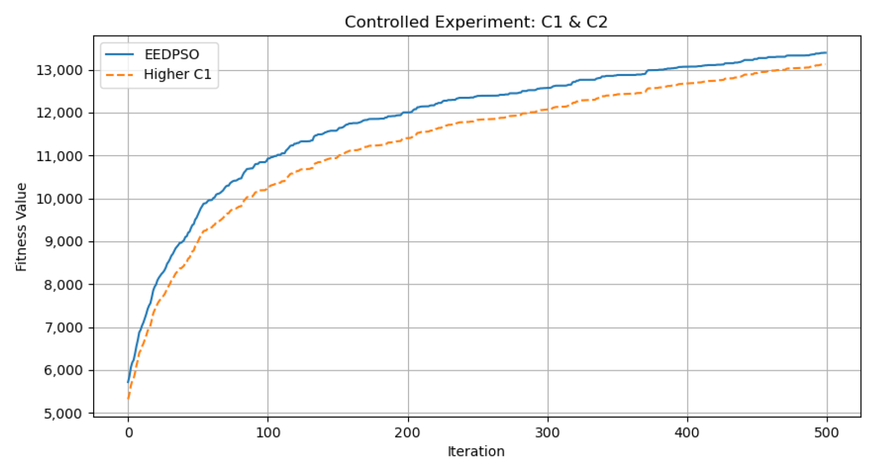
6.3. Distribution of Individual Learning Term (c1) and Global Learning Term (c2)

In particle swarm optimization (PSO), $c_1$ and $c_2$ regulate the balance between local and global search. A larger $c_1$ enhances local exploration by encouraging particles to revisit previously explored regions, but it also increases the risk of entrapment in local optima. Conversely, a larger $c_2$ accelerates convergence by directing particles toward the global best solution, although it may lead to premature convergence and insufficient exploration of the search space [63].

When $c_1+c_2>4$, particle trajectories may diverge, preventing convergence and leading to optimization failure. The optimal setting, typically $c_1=c_2=2.0$, ensures $c_1+c_2=4$, maintaining a critical balance between exploration and exploitation [63].

To investigate the influence of learning factors $c_1$ and $c_2$ and identify well-performing configurations for EEDPSO, we utilized the Optuna hyperparameter optimization framework. The search space was defined as $c_1,c_2\in [0.2,2.0]$, with an upper bound constraint of $c_1+c_2\le 4.0$ to ensure stability during search. Optuna employed the tree-structured Parzen Estimator (TPE) to efficiently sample promising parameter combinations. For each trial, the algorithm was run independently 100 times to reduce the influence of randomness, and the best fitness value among those runs was recorded as the objective metric. This process was repeated across more than 150 trials, allowing thorough exploration of the parameter landscape. The best configuration obtained was $c_1=1.26$, $c_2=0.74$, which was then adopted as the baseline in our subsequent control experiments. As evidenced in

Table 8. Control experiment of learning factors. Arrows indicate changes relative to baseline: "↑" for increase, "↓" for decrease.

Setting	Dimension	w	${\mathit{c}}_1$	${\mathit{c}}_2$	${\mathit{c}}_1+{\mathit{c}}_2$	Fitness
Baseline (EEDPSO)	200	0.55	1.26	0.74	2.00	13,394.04
C2↑, C1↓	200	0.55	0.74	1.26	2.00	12,858.28
C1↑, C2↓	200	0.55	1.46	0.54	2.00	13,126.16
C1↓, C2↔	200	0.55	0.40	0.80	1.20	11,742.51
C2↓, C1↔	200	0.55	0.80	0.40	1.20	11,875.97
Baseline (EEDPSO)	100	0.55	1.38	0.62	2.00	6560.22
C2↑, C1↓	100	0.55	0.98	1.02	2.00	6284.10
C1↑, C2↓	100	0.55	1.68	0.32	2.00	6622.71
C1↓, C2↔	100	0.55	0.40	0.80	1.20	5503.51
C2↓, C1↔	100	0.55	0.80	0.40	1.20	5620.32

and Figure 21 and Figure 22, different combinations of $c_1$ and $c_2$ produce noticeably different convergence behaviors and fitness outcomes. These findings demonstrate not only the sensitivity of EEDPSO to its learning factors but also the practical value of data-driven tuning strategies in enhancing the overall performance across varying problem scenarios.

We observe that increasing $c_2$ while decreasing $c_1$ accelerates early convergence (e.g., “Higher $c_2$” setting), reflecting stronger attraction toward the global best solution. However, this setting results in premature convergence and poorer final performance due to reduced population diversity. In contrast, a higher $c_1$ emphasizes personal learning, slightly improving late-stage convergence but causing slower early progress and less stable behavior overall.

Poor parameter settings clearly degrade performance. For instance, extremely low values lead to insufficient movement and slow convergence throughout, while excessively large values cause unstable particle trajectories and convergence failure. Symmetric configurations yield acceptable results but fail to exploit the dynamic strengths of either term.

The best performance was achieved using asymmetrical settings, specifically $c_1=1.26$ and $c_2=0.74$, in high-dimensional settings. This combination ensures strong global guidance with sufficient exploratory variability, balancing convergence speed and diversity.

Based on these results, we recommend the following guidelines for practitioners: In low-dimensional problems, slightly increasing $c_1$ to $1.1\sim 1.6$ and maintaining or slightly reducing $c_2$ to $0.4\sim 1.1$ helps to enhance early-stage local search and leads to better convergence performance, as confirmed by the improved fitness values in the 100-dimensional group. In high-dimensional problems (dimension $\ge 200$), it is more effective to reduce $c_1$ to $0.3\sim 0.8$ and increase $c_2$ to $1.2\sim 1.6$ to strengthen global learning and avoid premature local convergence. For noisy or heavily perturbed problems, $c_1$ should be reduced even further while keeping $c_2$ relatively high to stabilize the search process. In general, maintaining $c_1+c_2\approx 2.0$ achieves a good balance between exploration and exploitation across scenarios.

These findings confirm that, while EEDPSO retains the core roles of $c_1$ and $c_2$ from classical PSO, the optimal ranges shift due to the algorithm’s discrete design and enhanced local update mechanisms.

7. Conclusions

This paper introduces the elite evolutionary discrete particle swarm optimization (EEDPSO) algorithm, designed for solving RS and other combinatorial optimization problems. While preserving the key advantages of traditional PSO, the algorithm discretizes particle representation according to the problem’s data structure. An elite evolution strategy is employed through neighborhood exploration, effectively balancing local and global optimization. The particle velocity is redefined as a dimensional change, with the velocity update mechanism modified using Jaccard similarity and the position update enhanced by roulette-wheel selection, incorporating a perturbation value to promote exploration.

The experimental results demonstrate that EEDPSO significantly outperforms five mainstream metaheuristic algorithms in terms of both computational quality and convergence speed. Ablation studies and hyperparameter sensitivity analyses further confirm that this performance advantage stems from the algorithm’s internal design: the elite evolution strategy enhances solution development, while the coordination of velocity, position, and hyperparameters effectively balances global exploration and local exploitation. The optimization process reveals that improving one aspect often compromises another, highlighting the importance of maintaining equilibrium between exploration and exploitation. EEDPSO addresses this challenge by enhancing individual-level precision while preserving population diversity, enabling thorough local search without sacrificing the global search capability.

In deep recommendation system experiments, EEDPSO was compared with several representative deep recommendation models. The results show that, on sub-million-scale datasets, EEDPSO achieves superior performance. Even on million-scale datasets, it maintains comparable effectiveness while requiring lower training complexity and computational resources. The calculation accuracy is slightly lower than FairGo, and far better than the PRM without cold-start adaptation.

Thanks to its robustness in sparse and high-dimensional environments, EEDPSO proves to be an efficient solution for recommendation systems under cold-start conditions. Furthermore, its scalability and adaptability make it suitable for a variety of related applications, including personalized advertising, content recommendation, and short video feed ranking—domains where fast response and high accuracy are equally important [64].

Overall, these findings suggest that EEDPSO offers a practical and high-performance alternative to deep-learning-based methods in scenarios that demand lightweight, interpretable, and scalable recommendation solutions.

Despite its advantages, EEDPSO has certain limitations. Specifically, it may perform inefficiently in problems with relatively low dimensions or when the problem representation is binary as the search mechanism can become overly conservative, leading to lower efficiency [65]. Moreover, EEDPSO does not adapt well to combinatorial optimization problems that involve sequencing constraints, such as VRPs. Therefore, targeted optimizations are necessary to make the algorithm more suitable for such problems. In addition, in datasets of millions or more items, EEDPSO may lag behind some deep recommendation systems, so there is still potential for breakthrough.

Future work will focus on adapting the algorithm to new combinatorial optimization problems to enhance its versatility [66,67,68], such as Vehicle Routing Problems (VRPs) [69], Traveling Salesman Problems (TSPs), and other problems involving sequencing constraints. Another promising direction is to integrate deep recommendation systems [70], such as graph neural networks (GNNs), and incorporate user profiling to add personalized prediction features. This integration will aim to maintain the high performance of EEDPSO, particularly in cold-start scenarios.

References

1. Park, D.H.; Kim, H.K.; Choi, I.Y.; Kim, J.K. A literature review and classification of recommender systems research. Expert Syst. Appl. 2012, 39, 10059–10072. [Google Scholar] [CrossRef]
2. Lyu, Y. Recommender Systems in e-Commerce. In Proceedings of the 2021 International Conference on Intelligent Computing, Automation and Applications (ICAA), Nanjing, China, 25–27 June 2021; pp. 209–212. [Google Scholar] [CrossRef]
3. Lops, P.; de Gemmis, M.; Semeraro, G. Content-based Recommender Systems: State of the Art and Trends. In Recommender Systems Handbook; Springer: Boston, MA, USA, 2011; pp. 73–105. [Google Scholar] [CrossRef]
4. Wu, L.; Chen, L.; Shao, P.; Hong, R.; Wang, X.; Wang, M. Learning Fair Representations for Recommendation: A Graph-based Perspective. In Proceedings of the Web Conference 2021, Ljubljana, Slovenia, 19–23 April 2021; WWW ’21. ACM: New York, NY, USA, 2021; pp. 2198–2208. [Google Scholar] [CrossRef]
5. Pei, C.; Zhang, Y.; Zhang, Y.; Sun, F.; Lin, X.; Sun, H.; Wu, J.; Jiang, P.; Ge, J.; Ou, W.; et al. Personalized re-ranking for recommendation. In Proceedings of the 13th ACM Conference on Recommender Systems, Copenhagen, Denmark, 16–20 September 2019; RecSys ’19. ACM: New York, NY, USA, 2019; pp. 3–11. [Google Scholar] [CrossRef]
6. Bruun, S.B.; Leśniak, K.K.; Biasini, M.; Carmignani, V.; Filianos, P.; Lioma, C.; Maistro, M. Graph-Based Recommendation for Sparse and Heterogeneous User Interactions. In Proceedings of the Advances in Information Retrieval; Kamps, J., Goeuriot, L., Crestani, F., Maistro, M., Joho, H., Davis, B., Gurrin, C., Kruschwitz, U., Caputo, A., Eds.; Springer: Cham, Switzerland, 2023; pp. 182–199. [Google Scholar] [CrossRef]
7. Su, X.; Khoshgoftaar, T.M. A survey of collaborative filtering techniques. Adv. in Artif. Intell. 2009, 2009, 421425. [Google Scholar] [CrossRef]
8. Sengupta, S.; Basak, S.; Peters, R.A. Particle Swarm Optimization: A Survey of Historical and Recent Developments with Hybridization Perspectives. Mach. Learn. Knowl. Extr. 2019, 1, 157–191. [Google Scholar] [CrossRef]
9. Kennedy, J.; Eberhart, R. Particle swarm optimization. In Proceedings of the ICNN’95-International Conference on Neural Networks, Perth, Australia, 27 November–1 December 1995; Volume 4, pp. 1942–1948. [Google Scholar] [CrossRef]
10. Jain, M.; Saihjpal, V.; Singh, N.; Singh, S.B. An Overview of Variants and Advancements of PSO Algorithm. Appl. Sci. 2022, 12, 8392. [Google Scholar] [CrossRef]
11. Eberhart; Shi, Y. Particle swarm optimization: Developments, applications and resources. In Proceedings of the 2001 Congress on Evolutionary Computation (IEEE Cat. No.01TH8546), Seoul, Republic of Korea, 27–30 May 2001; Volume 1, pp. 81–86. [Google Scholar] [CrossRef]
12. Blum, C.; Roli, A. Metaheuristics in combinatorial optimization: Overview and conceptual comparison. ACM Comput. Surv. 2003, 35, 268–308. [Google Scholar] [CrossRef]
13. Yang, H.; Yu, Y.; Cheng, J.; Lei, Z.; Cai, Z.; Zhang, Z.; Gao, S. An intelligent metaphor-free spatial information sampling algorithm for balancing exploitation and exploration. Knowl.-Based Syst. 2022, 250, 109081. [Google Scholar] [CrossRef]
14. Marini, F.; Walczak, B. Particle swarm optimization (PSO). A tutorial. Chemom. Intell. Lab. Syst. 2015, 149, 153–165. [Google Scholar] [CrossRef]
15. Gad, A.G. Particle Swarm Optimization Algorithm and Its Applications: A Systematic Review. Arch. Comput. Methods Eng. 2022, 29, 2531–2561. [Google Scholar] [CrossRef]
16. Hao, Z.F.; Guo, G.H.; Huang, H. A Particle Swarm Optimization Algorithm with Differential Evolution. In Proceedings of the 2007 International Conference on Machine Learning and Cybernetics, Hong Kong, China, 19–22 August 2007; Volume 2, pp. 1031–1035. [Google Scholar] [CrossRef]
17. Peng, Z.; Al Chami, Z.; Manier, H.; Manier, M.A. A hybrid particle swarm optimization for the selective pickup and delivery problem with transfers. Eng. Appl. Artif. Intell. 2019, 85, 99–111. [Google Scholar] [CrossRef]
18. Bag, S.; Kumar, S.K.; Tiwari, M.K. An efficient recommendation generation using relevant Jaccard similarity. Inf. Sci. 2019, 483, 53–64. [Google Scholar] [CrossRef]
19. Črepinšek, M.; Liu, S.H.; Mernik, M. Exploration and exploitation in evolutionary algorithms: A survey. ACM Comput. Surv. 2013, 45, 1–33. [Google Scholar] [CrossRef]
20. Zhang, Y.; Wang, S.; Ji, G. A Comprehensive Survey on Particle Swarm Optimization Algorithm and Its Applications. Math. Probl. Eng. 2015, 2015, 931256. [Google Scholar] [CrossRef]
21. Tomar, V.; Bansal, M.; Singh, P. Metaheuristic Algorithms for Optimization: A Brief Review. Eng. Proc. 2023, 59, 238. [Google Scholar] [CrossRef]
22. Cui, J.s.; Shang, T.z.; Yang, F.; Yu, J.w. Ranking recommendation to implement meta-heuristic algorithm based on multi-label k-nearest neighbor method. Control. Decis. 2022, 37, 1289–1298. [Google Scholar] [CrossRef]
23. Li, G.; Zhang, T.; Tsai, C.Y.; Yao, L.; Lu, Y.; Tang, J. Review of the metaheuristic algorithms in applications: Visual analysis based on bibliometrics. Expert Syst. Appl. 2024, 255, 124857. [Google Scholar] [CrossRef]
24. Petroski Such, F.; Madhavan, V.; Conti, E.; Lehman, J.; Stanley, K.O.; Clune, J. Deep Neuroevolution: Genetic Algorithms Are a Competitive Alternative for Training Deep Neural Networks for Reinforcement Learning. arXiv 2017. [Google Scholar] [CrossRef]
25. Young, S.R.; Rose, D.C.; Karnowski, T.P.; Lim, S.H.; Patton, R.M. Optimizing deep learning hyper-parameters through an evolutionary algorithm. In Proceedings of the Workshop on Machine Learning in High-Performance Computing Environments, Austin, TX, USA, 15 November 2015; MLHPC ’15. ACM: New York, NY, USA, 2015. [Google Scholar] [CrossRef]
26. Cinar, A.C. A comprehensive comparison of accuracy-based fitness functions of metaheuristics for feature selection. Soft Comput. 2023, 27, 8931–8958. [Google Scholar] [CrossRef]
27. Alhijawi, B.; Kilani, Y. A collaborative filtering recommender system using genetic algorithm. Inf. Process. Manag. 2020, 57, 102310. [Google Scholar] [CrossRef]
28. Alhijawi, B.; Kilani, Y.; Alsarhan, A. Improving recommendation quality and performance of genetic-based recommender system. Int. J. Adv. Intell. Paradig. 2020, 15, 77–88. [Google Scholar] [CrossRef]
29. Boryczka, U.; Bałchanowski, M. Differential Evolution in a Recommendation System Based on Collaborative Filtering. In Proceedings of the Computational Collective Intelligence; Nguyen, N.T., Iliadis, L., Manolopoulos, Y., Trawiński, B., Eds.; Springer: Cham, Switzerland, 2016; pp. 113–122. [Google Scholar] [CrossRef]
30. Boryczka, U.; Bałchanowski, M. Speed up Differential Evolution for ranking of items in recommendation systems. Procedia Comput. Sci. 2021, 192, 2229–2238. [Google Scholar] [CrossRef]
31. Tlili, T.; Krichen, S. A simulated annealing-based recommender system for solving the tourist trip design problem. Expert Syst. Appl. 2021, 186, 115723. [Google Scholar] [CrossRef]
32. Ye, Z.; Xiao, K.; Ge, Y.; Deng, Y. Applying Simulated Annealing and Parallel Computing to the Mobile Sequential Recommendation. IEEE Trans. Knowl. Data Eng. 2019, 31, 243–256. [Google Scholar] [CrossRef]
33. Yang, S.; Wang, H.; Xu, Y.; Guo, Y.; Pan, L.; Zhang, J.; Guo, X.; Meng, D.; Wang, J. A Coupled Simulated Annealing and Particle Swarm Optimization Reliability-Based Design Optimization Strategy under Hybrid Uncertainties. Mathematics 2023, 11, 4790. [Google Scholar] [CrossRef]
34. Katarya, R.; Verma, O.P. A collaborative recommender system enhanced with particle swarm optimization technique. Multimed. Tools Appl. 2016, 75, 9225–9239. [Google Scholar] [CrossRef]
35. Kuo, R.; Li, S.S. Applying particle swarm optimization algorithm-based collaborative filtering recommender system considering rating and review. Appl. Soft Comput. 2023, 135, 110038. [Google Scholar] [CrossRef]
36. Gu, X.L.; Huang, M.; Liang, X. A Discrete Particle Swarm Optimization Algorithm with Adaptive Inertia Weight for Solving Multiobjective Flexible Job-shop Scheduling Problem. IEEE Access 2020, 8, 33125–33136. [Google Scholar] [CrossRef]
37. Zhou, T.; Su, R.Q.; Liu, R.R.; Jiang, L.L.; Wang, B.H.; Zhang, Y.C. Accurate and diverse recommendations via eliminating redundant correlations. New J. Phys. 2009, 11, 123008. [Google Scholar] [CrossRef]
38. Zhang, S.; Yao, L.; Sun, A.; Tay, Y. Deep Learning Based Recommender System: A Survey and New Perspectives. ACM Comput. Surv. 2019, 52, 1–38. [Google Scholar] [CrossRef]
39. Jannach, D.; Zanker, M.; Felfernig, A.; Friedrich, G. Recommender Systems: An Introduction, 1st ed.; Cambridge University Press: Cambridge, UK, 2010; Available online: https://dl.acm.org/doi/book/10.5555/1941904 (accessed on 21 December 2024).
40. Herlocker, J.L.; Konstan, J.A.; Terveen, L.G.; Riedl, J.T. Evaluating collaborative filtering recommender systems. ACM Trans. Inf. Syst. 2004, 22, 5–53. [Google Scholar] [CrossRef]
41. Lim, Y.J.; Teh, Y.W. Variational Bayesian approach to movie rating prediction. In Proceedings of the KDD Cup and Workshop, San Jose, CA, USA, 12–15 August 2007; Volume 7, pp. 15–21. Available online: https://www.cs.uic.edu/~liub/KDD-cup-2007/proceedings/variational-Lim.pdf (accessed on 4 January 2025).
42. Ning, X.; Karypis, G. SLIM: Sparse Linear Methods for Top-N Recommender Systems. In Proceedings of the 2011 IEEE 11th International Conference on Data Mining, Vancouver, BC, Canada, 11–14 December 2011; pp. 497–506. [Google Scholar] [CrossRef]
43. Yang, Y.; Li, H.; Lei, Z.; Yang, H.; Wang, J. A Nonlinear Dimensionality Reduction Search Improved Differential Evolution for large-scale optimization. Swarm Evol. Comput. 2025, 92, 101832. [Google Scholar] [CrossRef]
44. AlRashidi, M.R.; El-Hawary, M.E. A Survey of Particle Swarm Optimization Applications in Electric Power Systems. IEEE Trans. Evol. Comput. 2009, 13, 913–918. [Google Scholar] [CrossRef]
45. Raß, A.; Schmitt, M.; Wanka, R. Explanation of Stagnation at Points that are not Local Optima in Particle Swarm Optimization by Potential Analysis. In Proceedings of the Companion Publication of the 2015 Annual Conference on Genetic and Evolutionary Computation, Madrid, Spain, 11–15 July 2015; GECCO Companion ’15. ACM: New York, NY, USA, 2015; pp. 1463–1464. [Google Scholar] [CrossRef]
46. Ceschia, S.; Di Gaspero, L.; Rosati, R.M.; Schaerf, A. Reinforcement Learning for Multi-Neighborhood Local Search in Combinatorial Optimization. In Proceedings of the Machine Learning, Optimization, and Data Science; Nicosia, G., Ojha, V., La Malfa, E., La Malfa, G., Pardalos, P.M., Umeton, R., Eds.; Springer: Cham, Switzerland, 2024; pp. 206–221. [Google Scholar]
47. Shi, Y.; Eberhart, R. A modified particle swarm optimizer. In Proceedings of the 1998 IEEE International Conference on Evolutionary Computation Proceedings, IEEE World Congress on Computational Intelligence (Cat. No.98TH8360), Anchorage, AK, USA, 4–9 May 1998; pp. 69–73. [Google Scholar] [CrossRef]
48. Lipowski, A.; Lipowska, D. Roulette-wheel selection via stochastic acceptance. Phys. A Stat. Mech. Its Appl. 2012, 391, 2193–2196. [Google Scholar] [CrossRef]
49. Shi, Y.; Eberhart, R. Empirical study of particle swarm optimization. In Proceedings of the 1999 Congress on Evolutionary Computation-CEC99 (Cat. No. 99TH8406), Washington, DC, USA, 6–9 July 1999; Volume 3, pp. 1945–1950. [Google Scholar] [CrossRef]
50. movielens. movielens-20m. Available online: https://files.grouplens.org/datasets/movielens/ml-20m-README.html (accessed on 3 December 2019).
51. movielens. movielens-32m. Available online: https://files.grouplens.org/datasets/movielens/ml-32m-README.html (accessed on 13 October 2023).
52. Jianmo Ni, U. Amazon Review Data (2018). Available online: https://nijianmo.github.io/amazon/index.html (accessed on 8 August 2020).
53. Goldberg, D.E. Genetic Algorithms in Search, Optimization and Machine Learning, 1st ed.; Addison-Wesley Longman Publishing Co., Inc.: Boston, MA, USA, 1989; Available online: https://dl.acm.org/doi/book/10.5555/534133 (accessed on 9 December 2024).
54. Assad, A.; Deep, K. A Hybrid Harmony search and Simulated Annealing algorithm for continuous optimization. Inf. Sci. 2018, 450, 246–266. [Google Scholar] [CrossRef]
55. Tanabe, R.; Fukunaga, A. Success-history based parameter adaptation for Differential Evolution. In Proceedings of the 2013 IEEE Congress on Evolutionary Computation, Cancun, Mexico, 20–23 June 2013; pp. 71–78. [Google Scholar] [CrossRef]
56. Bilal; Pant, M.; Zaheer, H.; Garcia-Hernandez, L.; Abraham, A. Differential Evolution: A review of more than two decades of research. Eng. Appl. Artif. Intell. 2020, 90, 103479. [Google Scholar] [CrossRef]
57. Mirjalili, S. SCA: A Sine Cosine Algorithm for solving optimization problems. Knowl.-Based Syst. 2016, 96, 120–133. [Google Scholar] [CrossRef]
58. Suman, B.; Kumar, P. A survey of simulated annealing as a tool for single and multiobjective optimization. J. Oper. Res. Soc. 2006, 57, 1143–1160. [Google Scholar] [CrossRef]
59. Akiba, T.; Sano, S.; Yanase, T.; Ohta, T.; Koyama, M. Optuna: A Next-generation Hyperparameter Optimization Framework. In Proceedings of the 25th ACM SIGKDD International Conference on Knowledge Discovery & Data Mining, Anchorage, AK, USA, 4–8 August 2019; KDD ’19. ACM: New York, NY, USA, 2019; pp. 2623–2631. [Google Scholar] [CrossRef]
60. Wang, M.; Zheng, S.; Li, X.; Qin, X. A new image denoising method based on Gaussian filter. In Proceedings of the 2014 International Conference on Information Science, Electronics and Electrical Engineering, Sapporo, Japan, 26–28 April 2014; Volume 1, pp. 163–167. [Google Scholar] [CrossRef]
61. Huang, X.; Zhao, F.; An, J. Review on Similarity Calculation of Recommendation Algorithms. Oper. Res. Fuzziol. 2022, 12, 119–124. [Google Scholar] [CrossRef]
62. Xu, H.; Deng, Q.; Zhang, Z.; Lin, S. A hybrid differential evolution particle swarm optimization algorithm based on dynamic strategies. Sci. Rep. 2025, 15, 4518. [Google Scholar] [CrossRef]
63. Clerc, M.; Kennedy, J. The particle swarm - explosion, stability, and convergence in a multidimensional complex space. IEEE Trans. Evol. Comput. 2002, 6, 58–73. [Google Scholar] [CrossRef]
64. Ko, H.; Lee, S.; Park, Y.; Choi, A. A survey of recommendation systems: Recommendation models, techniques, and application fields. Electronics 2022, 11, 141. [Google Scholar] [CrossRef]
65. Yang, H.; Gao, S.; Lei, Z.; Li, J.; Yu, Y.; Wang, Y. An improved spherical evolution with enhanced exploration capabilities to address wind farm layout optimization problem. Eng. Appl. Artif. Intell. 2023, 123, 106198. [Google Scholar] [CrossRef]
66. Yang, Y.; Tao, S.; Li, H.; Yang, H.; Tang, Z. A Multi-Local Search-Based SHADE for Wind Farm Layout Optimization. Electronics 2024, 13, 3196. [Google Scholar] [CrossRef]
67. Nagata, Y. High-Order Entropy-Based Population Diversity Measures in the Traveling Salesman Problem. Evol. Comput. 2020, 28, 595–619. [Google Scholar] [CrossRef] [PubMed]
68. Nagata, Y.; Imahori, S. Creation of Dihedral Escher-like Tilings Based on As-Rigid-As-Possible Deformation. ACM Trans. Graph. 2024, 43, 1–18. [Google Scholar] [CrossRef]
69. Konstantakopoulos, G.D.; Gayialis, S.P.; Kechagias, E.P. Vehicle routing problem and related algorithms for logistics distribution: A literature review and classification. Oper. Res. 2022, 22, 2033–2062. [Google Scholar] [CrossRef]
70. Yang, H.; Yang, Y.; Zhang, Y.; Tang, C.; Hashimoto, K.; Nagata, Y. Chaotic Map-Coded Evolutionary Algorithms for Dendritic Neuron Model Optimization. In Proceedings of the 2024 IEEE Congress on Evolutionary Computation (CEC), Yokohama, Japan, 30 June–5 July 2024; pp. 1–8. [Google Scholar] [CrossRef]
Figure 1. Data form in which users rate items.
Mathematics 13 01398 g001
Figure 2. Rating number and average rating.
Mathematics 13 01398 g002
Figure 3. Fitness calculation process.
Mathematics 13 01398 g003
Figure 4. Description of the EEDPSO.
Mathematics 13 01398 g004
Figure 5. Roulette-wheel position update.
Mathematics 13 01398 g005
Figure 6. Scatter plot of hyperparameter search for EEDPSO in MovieLens-20M.
Mathematics 13 01398 g006
Figure 7. Convergence curves of MovieLens.
Mathematics 13 01398 g007
Figure 8. Convergence curves of AmazonReviewData.
Mathematics 13 01398 g008
Figure 9. Box plot of MovieLens.
Mathematics 13 01398 g009
Figure 10. Box plot of AmazonReviewData.
Mathematics 13 01398 g010
Figure 11. Distribution chart of MovieLens.
Mathematics 13 01398 g011
Figure 12. Distribution chart of AmazonReviewData.
Mathematics 13 01398 g012
Figure 13. Scatter plot of MovieLens.
Mathematics 13 01398 g013
Figure 14. Scatter plot of AmazonReviewData.
Mathematics 13 01398 g014
Figure 15. Ablation experiment curve.
Mathematics 13 01398 g015
Figure 16. Ablation experiment slope diagram.
Mathematics 13 01398 g016
Figure 17. Analysis of the results of ablation experiment.
Mathematics 13 01398 g017
Figure 18. Velocity change curve chart.
Mathematics 13 01398 g018
Figure 19. Comparison of curves in EEDPSO.
Mathematics 13 01398 g019
Figure 20. Comparison of curves in EEDPSO3.
Mathematics 13 01398 g020
Figure 21. Graph of higher C1.
Mathematics 13 01398 g021
Figure 22. Graph of higher C2.
Mathematics 13 01398 g022