Abstract
The estimation of drift parameters in the Ornstein–Uhlenbeck (O-U) process with jumps primarily employs methods such as maximum likelihood estimation, least squares estimation, and least absolute deviation estimation. These methods generally assume specific error distributions and finite variances. However, with the increasing uncertainty in financial markets, asset prices exhibit characteristics such as skewness and heavy tails, which lead to biases in traditional estimators. This paper proposes a self-weighted quantile estimator for the drift parameters of the O-U process with jumps and verifies its asymptotic normality under large samples, given certain assumptions. Furthermore, through Monte Carlo simulations, the proposed self-weighted quantile estimator is compared with least squares, quantile, and power variation estimators. The estimation performance is evaluated using metrics such as mean, standard deviation, and mean squared error (MSE). The simulation results show that the self-weighted quantile estimator proposed in this paper performs well across different metrics, such as 8.21% and 8.15% reduction of MSE at the 0.9 quantile for drift parameter and compared with the traditional quantile estimator. Finally, the proposed estimator is applied to inter-period statistical arbitrage of the CSI 300 Index Futures. The backtesting results indicate that the self-weighted quantile method proposed in this paper performs well in empirical applications.
Keywords:
self-weighted quantile estimation; drift coefficients; O-U process with jumps; heavy-tailed distributions; statistical arbitrage; asymptotic normality; Monte Carlo simulations MSC:
62M05; 60J75; 62P20
1. Introduction
The Ornstein–Uhlenbeck (O-U) process is a stochastic process that exhibits mean-reverting characteristics, and its parameter estimation problem is an important research area in the statistical inference of stochastic processes. In the 21st century, the parameter estimation problem of the O-U process has been widely developed, with the main research achievements including the following:
- MCMC methods (Griffin, Steel [1], Roberts, Papaspiliopoulos [2]) that use Markov chain Monte Carlo simulation to estimate parameters;
- Nonparametric methods (Jongbloed [3]);
- Parametric methods (Valdivieso [4], Valdivieso [5]). The main estimation methods focus on the maximum likelihood estimation (MLE) and least squares estimation (LSE).
As the driving process of the O-U process evolves from continuous to discrete, from Wiener process to Lévy-driven, and from Gaussian to non-Gaussian, the O-U-type process gradually becomes more precise in describing actual market data. However, the early statistical inference methods and conclusions face certain difficulties and resistance when extended to these new O-U processes, and are less effective in the statistical inference of new O-U processes. Therefore, there are relatively few theories and methods that can be directly applied to these new O-U processes. The Lévy-driven O-U process was first proposed by Barndorff-Nielsen and Shephard [6] and has been widely used in the modeling of financial asset return volatility. In the parameter estimation problem of the Lévy-driven O-U process, most previous work has focused on special types of Lévy processes driving the O-U process, such as non-negative Lévy processes (Jongbloed et al. [3], Jongbloed and Van Der Meulen [7], Zhang et al. [8], Brockwell et al. [9], Leonenko et al. [10]), compound Poisson processes (Zhang [11], Wu et al. [12]), -stable Lévy processes (Hu and Long [13], Zhang [14]), Lévy processes composed of Wiener process and -stable Lévy process (Long [15]), heavy-tailed symmetric Lévy processes (Masuda [16]), and Lévy processes without Brownian motion component (Taufer and Leonenko [17], Valdivieso et al. [17]). For the parameter estimation methods of these special types of Lévy–O-U processes, they mainly still focus on least squares and maximum likelihood methods. Hu and Long [18] used a combination of trajectory fitting method and weighted least squares method to discuss the consistency and asymptotic distribution of the estimators of the O-U equation driven by -stable Lévy motion in both ergodic and non-ergodic cases. Subsequently, Hu and Long [13] studied the parameter estimation problem of the generalized O-U equation driven by -stable noise at discrete time points. Masuda [16] introduced LAD estimation into the drift parameter estimation of general Lévy–O-U processes, and then found that the SLAD estimator has a limit distribution, satisfies asymptotic properties, and is robust to large “jumps” in the driving process. Mai [19] developed an estimator based on the maximum likelihood estimation method for the drift parameter. Spiliopoulos [20] derived the estimators of the drift parameter and other parameters related to the Lévy process for the O-U process driven by a general Lévy process based on the moment estimation method. Wu and Hu [21] proposed a moment estimator for the drift parameter of the O-U process driven by a general Lévy process, derived the asymptotic variance, and proved the central limit theorem. Shu [22] et al. proposed a trajectory fitting estimator for the drift parameter of the O-U process driven by small Lévy noise and proved its consistency and asymptotic distribution. Wang [23] et al. constructed a fractional Ornstein–Uhlenbeck model driven by tempered fractional Brownian motion. They derived the least squares estimator for the drift parameter based on discrete observations and proved its consistency and asymptotic distribution. Han [24] proposed a modified least squares estimator for estimating the drift parameter of the Ornstein–Uhlenbeck process from low-frequency observations and proved the strong consistency and joint asymptotic normality. Fares [25] investigated the strong consistency and asymptotic normality of the least squares estimator for the drift coefficient of complex-valued Ornstein–Uhlenbeck processes driven by fractional Brownian motion. Zhang [26] proposed the modified least squares estimators (MLSEs) for the drift parameters and a modified quadratic variation estimator (MQVE) for the diffusion parameter. The study leverages the ergodic properties of the O-U process to prove the asymptotic unbiasedness and normality of these estimators, and validates their effectiveness through Monte Carlo simulations.
Statistical arbitrage is a strategy that uses statistical methods and mathematical models to find inconsistencies in market price fluctuations, identify pricing errors or price deviations from normal levels in the market, and thus implement arbitrage operations in investment portfolios. Board [27] used cointegration techniques to arbitrage the price spread of the Nikkei 225 Index Futures across markets such as Singapore and Osaka, Japan, and found that there was indeed arbitrage space. Bondarenko [28] was the first to propose the concept of statistical arbitrage, and subsequently Hogan [29] summarized the definition of statistical arbitrage based on the definition of risk-free arbitrage, which has been widely used. Alexander [30] applied the statistical arbitrage strategy based on cointegration methods to the study of index tracking portfolios, and their empirical results showed that the arbitrage strategy based on cointegration methods had low volatility, low correlation with the market, and nearly normally distributed characteristics. Elliot [31] et al. proposed that due to the mean-reverting characteristics of the O-U process, it can be used to describe the mean-reverting nature of the spread sequence in statistical arbitrage. Bertram [32] gave the optimal solution of the trading signal when the stock price follows the O-U process. Rudy et al. [33] used high-frequency minute data for statistical arbitrage and found that the cointegration degree of the paired assets was positively correlated with arbitrage opportunities and returns. Wale conducted statistical arbitrage research on the US Treasury futures market and obtained significant excess returns, indicating that the US Treasury market had phenomena such as incomplete market efficiency and information asymmetry. Fang Hao [34] simulated and tested with Chinese closed-end funds, and discussed the possible situations of statistical arbitrage in practice according to the steps of selecting arbitrage objects, establishing arbitrage signal mechanisms, and establishing trading portfolios, proving that statistical arbitrage strategies are effective in the Chinese closed-end fund market. Calderia [35] constructed a cross-period arbitrage model combining cointegration theory for futures contracts with different maturities, and found that the price spread sequence of the same futures had a cointegration relationship and there was a large arbitrage space. Zhu Lirong et al. [36] designed a statistical arbitrage strategy for the domestic futures market, and the empirical results showed that stable returns could be obtained during the trading test period. Fan [37] found that the error obtained by the traditional cointegration model was non-stationary when looking for arbitrage opportunities between soybean oil and palm oil futures, so the Bayesian method was added to estimate the error, making the estimated parameters more sensitive and thus obtaining a larger expected return. Wang Jianhua, Cui Wenjing et al. [38] used the time-varying coefficient cointegration regression model to detect the structural breakpoints of financial time series, and established a cointegration statistical arbitrage model based on high-frequency data for IF1707 and IF1706 futures contracts. The results showed that the model was significantly better than the arbitrage performance of the ordinary cointegration model. Liu Yang, Lu Yi [39] selected the daily closing prices of the financial stock index futures of the Shanghai Stock Index 50 and the 50ETF to establish a dynamic statistical arbitrage model based on the O-U process, and determined the optimal trading signal and arbitrage interval under the goal of maximizing the expected return function. According to the performance of the arbitrage strategy, the O-U process is suitable for describing financial time series. Zhang Long [40] introduced the O-U process into the cross-commodity arbitrage of futures, taking palm oil and soybean oil as the modeling targets. Wu et al. [41] and Piergiacomo [42] showed that the simple O-U process has certain limitations in fitting the stock market spread sequence data, and cannot accurately fit the jump phenomena in the data sequence. The use of double exponential discrete jumps in the O-U process can significantly improve this deficiency. Zhao Hua, Luo Pan et al. [43] studied the high-frequency paired trading strategy in the Chinese stock market based on the Lévy–O-U process, and screened out stock pairs by estimating the mean reversion rate and realized volatility.
This paper systematically combs and reviews the literature on jump behavior, parameter estimation of jump O-U process, and statistical arbitrage. This literature has great inspirational significance for the development of this paper, but it cannot be denied that there are still some shortcomings in these studies.
- In the research on parameter estimation of jump O-U process, the least squares estimation method based on the square loss function and maximum likelihood estimation method have good estimation performance under the assumption of specific error distribution and finite variance. Under the finite variance scenario, the LSE based on the assumption of normal distribution of errors has asymptotic normality and optimal convergence rate but is sensitive to outliers. The maximum likelihood estimation also possesses large-sample asymptotic properties under the assumptions of distribution and finite variance. However, when the assumption conditions are relaxed to infinite variance, these estimators have problems that the asymptotic properties cannot be proved and the estimation is not robust. Under the premise of infinite variance, some scholars have proposed the self-weighted least absolute deviation estimator of the drift parameter and proved its good properties. It is found that the weighted least absolute deviation estimator is more robust to outliers. As a special case of the self-weighted quantile estimation 0.5 quantile, it can be further extended to various quantiles of self-weighted quantile, which can further improve the estimation accuracy and has large room for improvement.
- In the research on statistical arbitrage, many scholars have designed arbitrage strategies based on cointegration theory, GARCH, and O-U process, and the estimation methods used are mainly OLS and MLE. With the development of high-frequency trading, the data used gradually turns to high-frequency. However, existing research lacks consideration of the possible jumps and heavy tails in the price spread sequence of paired assets, and still uses traditional estimation methods to estimate and construct trading signals, which will cause the trading signals to deviate greatly, miss potential arbitrage opportunities, and weaken the overall performance of the strategy. Therefore, considering jumps and corresponding robust estimation methods to establish statistical arbitrage models, so that the models are closer to the real situation, is an issue worth paying attention to and improving in the design of statistical arbitrage strategies.
Based on these considerations, this paper proposes a self-weighted quantile estimation method for the O-U process with jumps under both finite and infinite variance scenarios, estimating the drift parameters for the pure jump structure O-U process. On one hand, the self-weighted quantile estimator does not rely on assumptions about the data distribution and provides a more comprehensive description of the distribution characteristics by offering confidence intervals and probability distributions at different quantiles, thus providing more complete uncertainty information. On the other hand, it further reduces the impact of outliers through weighting while being insensitive to them. Finally, by proving its asymptotic normality under the infinite variance scenario, the excellent properties of the self-weighted quantile estimator are demonstrated.
The structure of the paper is organized as follows. Section 2 proposes a self-weighted quantile estimator for the drift parameters, laying the groundwork for the proof of the conclusion. Section 3 proves its asymptotic normality and conducts Monte Carlo simulations to evaluate the performance of the proposed estimator. Section 4 applies the method to statistical arbitrage on the CSI 300 Index Futures and presents backtesting results. Section 5 concludes the paper.
2. Preliminaries
2.1. The O-U Process with Jump and Estimation Methods
The Ornstein–Uhlenbeck process is a type of diffusion process in physics, which is an odd-order Markov process with mean-reverting characteristics, suitable for capturing typical features of financial data, including mean reversion, volatility clustering, drift, and jumps.
The O-U process is defined by the following stochastic differential equation:
where represents the instantaneous drift parameter, represents the mean reversion strength, is the diffusion parameter, , is a standard Brownian motion, and is a jump component. The jump structure is diverse, mainly including Gaussian and Poisson structures, etc. It is commonly represented by a compound Poisson process with a jump intensity , where the jump size follows a normal distribution and is independent of . is a Lévy process. Typically, we estimate the unknown parameters based on discrete-time samples , where is the time interval between adjacent samples, also denoted as , with h being the fixed sampling grid. Parameters and are both drift parameters, describing the overall trend of the random variables in the stochastic process, representing the average growth rate or average drift speed of the stochastic process.
For the estimation of unknown parameters , the simplest and most common method is to use the approximate least squares estimator (LSE), by minimizing the following squared loss function:
The LSE estimator is obtained. Under the squared loss function, the difference between normal values and abnormal values will be amplified, making the model more sensitive to abnormal values, and abnormal values will receive more attention. The estimator satisfies asymptotic normality when Z has finite variance and its convergence rate is , which is the optimal convergence rate in the estimation of diffusion drift with Poisson jumps. However, when Z has infinite variance, the premise assumption that the error obeys a normal distribution is broken, and the situation is no longer the case.
In addition, the least absolute deviation estimator (LAD) can be used, by minimizing the following absolute value loss function:
The LAD estimator is obtained. Compared with the squared loss function, the absolute value loss function does not amplify the difference between normal values and outliers, so the impact of outliers on the model is smaller, and the model is more robust. The estimator converges to the normal distribution at a rate of when the error term has sufficiently high-order finite moments, but it is difficult to derive the specific form of its asymptotic normal distribution in the case of infinite variance. In addition to estimating parameters by minimizing the loss function, the maximum likelihood estimation method based on the probability distribution of data can also be used, which is usually maximized by numerical optimization algorithms to maximize the likelihood function of the observed data. Usually, the above common estimators can estimate the unknown parameters under the asymptotic properties of large samples, but their estimation effects are limited by the structure of the jump term. When it is a pure jump, its estimation effect is proved to be not as good as the case of simple distribution jumps, especially the appearance of large jumps, which makes the robustness of simple estimators impacted.
2.2. Optimal Trading Trigger Points
First, let us clarify that the trading objective of this paper is to maximize the expected return per unit time. Let the time interval of a trading cycle be T, which is a random variable. a and m (assuming ) are the trading signal trigger points. When the spread is equal to a, enter the trade; when it is equal to m, reverse the trade. The spread sequence is equal to a again, then the process from a to m and back to a constitutes a trading cycle . Assume the profit function within a trading cycle is , where c is the transaction cost, then the objective function is expressed as
Assume that the spread sequence of the paired assets follows the following O-U process:
At this time, according to the state of the transaction, it is divided into and , where represents the holding time from a to m, and represents the time from m to a. Since is a Markov process, and are independent of each other, therefore, in a complete trading process, we have
According to Itô’s lemma, after variable substitution for , the mean time interval of a trading cycle can be expressed as
where is the imaginary error function, and its derivative is .The target function for the unit time return within a trading cycle is
To find the maximum value of Equation (8), we take partial derivatives with respect to a and m, respectively:
Solving the above equations yields
2.3. Construction of the Self-Weighted Quantile Estimator of Drift Parameters for the O-U Process with Jumps
Assume is a univariate O-U process with jumps given by the following stochastic differential equation:
where is the instantaneous drift parameter, is the mean reversion strength, and is a Lévy process independent of . We denote the Lévy measure and Gaussian variance of by and , respectively, and assume to exclude trivial cases. Referring to Sato [44] for a systematic description of Lévy processes, we define the activity index to measure the degree of small jump fluctuations:
Compared to specific distribution structures such as Gaussian or Poisson structures, this structure is more general, and its specific characteristics are seen in Assumption 6. Let represent the true distribution of X related to , and be the corresponding expectation. Under the distribution , Equation (14) has the following autoregressive representation:
For convenience, let
To derive the conditional quantile function, assume that for any and , has a positive smooth Lebesgue density on , is independent of i, and is symmetric about 0. Then, the distribution of is . For any , given , we require that the conditional quantile function of satisfies . Then for any , we define the quantile loss function for the O-U process with jumps as
where is the quantile loss function, and is the weight function, whose specific form is seen in Assumption 7. Based on the goal of minimizing the loss function, the quantile estimator for the drift parameter is
Self-weighted quantile estimation is an advanced statistical technique that adjusts the traditional quantile estimation process by incorporating observation-specific weights. These weights are typically derived from the data itself, often reflecting the relative importance, reliability, or inverse variance of each observation. The method is particularly useful in contexts where data points are heteroskedastic (exhibit non-constant variance) or when certain observations should influence the quantile estimates more than others due to domain-specific considerations.
Traditional quantile estimation assumes homoskedasticity (constant variance). In financial or risk modeling, volatility clustering is common, and self-weighted methods adapt by down-weighting high-volatility periods. Self-weighting can reduce the influence of outliers by assigning them lower weights (e.g., based on Mahalanobis distance or residual analysis). Weights can evolve over time (e.g., time-decaying weights for older data), enabling the estimator to prioritize recent observations without discarding older data entirely. Moreover, the weights can incorporate domain knowledge (e.g., higher weights for liquid assets in portfolio risk models) or model confidence (e.g., inverse prediction error).
2.4. Assumptions
Let X be given by Equation (14), and let represent the initial distribution of X. Assume the following:
- There exists a constant such that ;
- Assume is a bounded convex set, whose closure ;
- As , the time interval and ;
- , given Assumption 3 that ;
- is the unique invariant distribution of X independent of , which is exponentially absolutely regular under , and satisfies and . The characteristic function of is
- The structure of is the following:
- (a)
- v is symmetric about the origin, and there exists a constant such that . The characteristic function of is
- (b)
- If , then can be represented by two Lévy measures and , which satisfy the following conditions:
- i.
- has a symmetric density function on , where , and as ,
- ii.
- ;
- The structure of the weight w is described as follows:
- (a)
- w is a bounded and uniformly continuous function;
- (b)
- , in particular, if for any , then the weight function is uniformly continuous.
Remark 1.
Assumptions 1 and 2 are the same assumptions for X be given by Equation (14) used in Masuda [16]. Assumptions 3 and 4 on sample size and bandwidth are sufficient. Note that it suffices that when while a faster decay of , i.e., is required when Assumption 5 is some facts concerning the O-U processes; see Masuda [45] for more details. Assumption 6 entails that small fluctuations of Z should be like that of a -stable Lévy process. In the self-weighting method, Assumption 7 is usually a necessary condition, which can reduce the impact of outliers by selecting appropriate weights. Inspired by Ling [46], we consider the following weight function:
where , is the 0.95 quantile of . This weight satisfies the requirements of Assumption 7, with a value range from 0 to 1, which can reduce the weight of estimators with outliers and has no effect on estimators without outliers. It implies that this weight can down-weight covariance matrices with outliers, and at the same time, it has no effect on the estimation results when there is no outlier.
2.5. Lemmas and Theorems
Let denote the r-dimensional normal distribution with mean vector and covariance matrix U, and let denote the symmetric -stable density function corresponding to when , and the Lévy density when . This implies
Lemma 1
(Hjørt and Pollard [47]). Let be a real-valued convex random function defined on a convex domain , and assume can be expressed as , where converges weakly to a random variable , converges in probability to a positive definite matrix , and for any , converges in probability to 0. Then the minimum value of converges weakly to .
Lemma 2
(Masuda [16]). Under Assumption 6, we have a uniform estimate , where is the symmetric stable density of β, d is a positive constant, and the values of d are as follows:
- 1.
- When or , ;
- 2.
- For any , if , then ;
- 3.
- For any , if , then ;
- 4.
- For any , if , then ;
- 5.
- For any and , if , then .
Lemma 3
(Masuda [16]). If Assumption 7 holds, and for some , , then for and , let
then .
Theorem 1.
Under the Assumption 2.4, for any , as ,
where , and are positive definite symmetric matrices, defined as follows:
Remark 2.
To make Theorem 1 applicable in practice, we must estimate , , and . Since and are represented by , according to Lemma 3, it is easy to obtain the uniform estimators for and as . For , since the density function of is symmetric, we can shift the τ quantile of to 0 such that , where . According to Lemma 2, the estimation of is transformed into the estimation of . According to Equation (23), depends only on the two parameters β and c. Using the uniform estimator of demonstrated in Theorem 1 of Masuda [16], we can use this uniform estimator without directly estimating β and c, thus obtaining all the estimators needed for the normal distribution.
Corollary 1.
Under the Assumption 2.4, for any , as n
3. Main Results
3.1. Theoretical Proofs
For the drift parameter self-weighted quantile estimator, this paper considers the proof of its asymptotic normality.
Proof of Theorem 1.
Let , according to Lemma 1, we construct a function about u. According to Equations (16)–(19), we have
According to the definition of the loss function, for any , we have
Let , where . Define the function :
Then , and we will prove that its minimum value is .
First, we provide the asymptotic local quadratic structure of . For any , we have
According to Lemma 1, we need to prove that and .
Next, we infer the specific local quadratic structure of Equation (28). For any K-function of the form , we have . Referring to Knight [48], taking , we have the formula
Let , , then we examine the asymptotic behavior of . Decompose as follows:
Denote for any matrix A, then
Since is bounded, and
we have
Now we note that the mixing property of X under the distribution leads to the ergodic theorem, that is, for each integrable function F, . Combining Lemma 3, we get , therefore,
Similarly, under these assumptions, it is easy to see that for any ,
From Equations (38) and (39), applying the Martingale central limit theorem to , we get . According to Equation (35), it is clear that . Therefore, , and for any u, .
Next, we examine the asymptotic behavior of . We separate the Martingale term of to get
For the first term on the right-hand side, according to Taylor’s formula, we have
Therefore, with the help of Lemmas 2 and 3, we have . For the term , first, according to Lemma 2, we have . Second, for any and , , we can obtain the following estimate:
Therefore, for any u, . For the second term of , let
Using Burkholder’s inequality and Schwarz’s inequality, we have
Therefore, for any u, and .
In summary, combining the asymptotic behaviors of and , we obtain Equation (28), and Theorem 1 is proved. □
Proof of Corollary 1.
Based on Theorem 1 and continuous mapping theorem, it is known that when , we have
That is, for every real number x, it holds that
Here, represents the distribution function of the normal distribution :
It is known that for any positive number , it holds that
Consider
thus,
It can be seen that it is only necessary to prove
and
For any positive number , since
take a sufficiently large real number such that
obviously such M exists, the larger the better. For the chosen , there naturally exists a positive integer , such that when , it holds that . Thus, when ,
Furthermore,
Additionally, due to the arbitrariness of , it is known that
By the same reasoning,
□
Similarly, it can be proven that
3.2. Monte Carlo Numerical Simulation
Based on the proof of the self-weighted quantile estimation method for the O-U process with jumps in the previous chapter, this chapter discusses the simulation and implementation of the fitting estimation algorithm for the O-U process with jumps. The simulation results are an important tool for subsequent evaluation of the quality of the estimators. We use Monte Carlo numerical simulations to study the properties of the weighted quantile estimators for the O-U process with jumps and compare them with the estimators obtained from quantile estimation methods, power variation estimation methods, and least squares estimation. In the simulation process, the O-U process with jumps is first discretized using the Euler method to generate a discrete O-U process with known parameters. Based on the simulated data, the drift parameters are estimated, and then the differences between the estimated values and the true values are compared. The accuracy and efficiency of the algorithm are evaluated using indicators such as mean, standard deviation, and mean squared error.
3.2.1. Sample Path Simulation
The sample path simulation equation for the O-U process with jumps is defined as follows:
When estimating the drift parameter, according to the assumption of the jump term structure in Section 2.3, take this distribution as , whose density is . Set the true parameter values as , the time interval , perform Monte Carlo simulations of sample paths, and each path contains observations. According to the Euler iteration, the simulated path of the random array following the above NIG jump structure O-U process is shown below:
As shown in Figure 1, the random array generated by model (58) exhibits certain fluctuation characteristics and obvious jump phenomena. In the actual financial market, when encountering information shocks or policy impacts, there are indeed significant jumps in intra-day high-frequency data, so our simulated paths can reflect the true characteristics of financial market data.
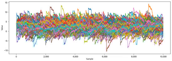
Figure 1.
Simulated path of O-U process with NIG jumps.
3.2.2. Method Comparison and Result Evaluation
Unlike other estimators, quantile estimation divides the data into several parts, each containing a certain proportion of data points, and focuses on describing the location and distribution of the data by estimating the quantiles. Therefore, we select as six quantile points to observe the data distribution. Based on the assumption of the weight structure, we choose an appropriate weight function to reduce the impact of abnormal observations on the estimation results, and it has no effect on the estimation of normal observations. Referring to Ling [46], consider the following weight function:
where , is the 0.95 quantile of . Combining settings of the path parameter and the estimator, perform self-weighted quantile estimation for each simulated path, and calculate the mean, standard deviation, and MSE of the estimated values for evaluation.
3.2.3. Comparison of Estimation Results for Drift Parameters
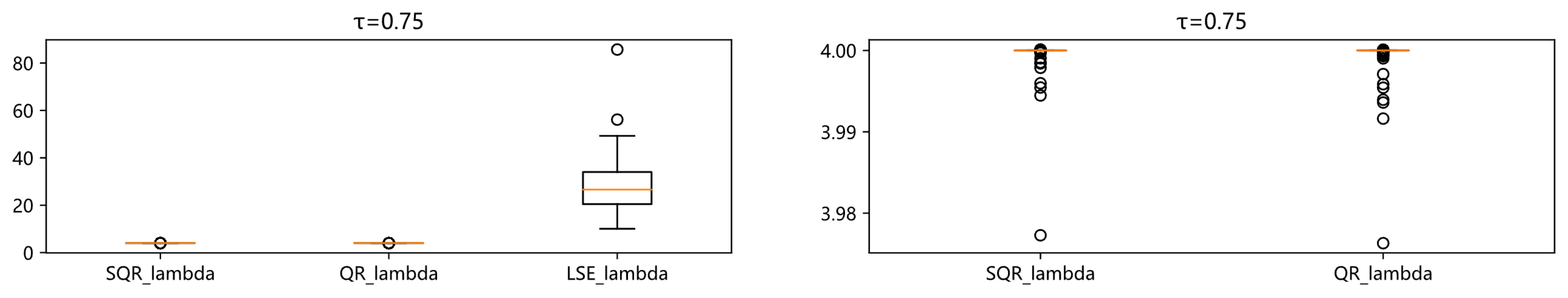
For the finite sample estimation effect of the drift parameters, consider the quantile estimation and least squares estimation as comparative estimation methods. Compared with the quantile and least squares estimators, the self-weighted quantile estimator can better estimate the drift parameters of the O-U process with specific jump structures. The Monte Carlo simulation results for the two drift parameters to be estimated are given in Table 1, Table 2, Table 3 and Table 4, and visualized by drawing box plots, as shown in Figure 2 and Figure 3.

Table 1.
Monte Carlo simulation results for drift parameter .
Table 2.
Monte Carlo simulation results for drift parameter .
Table 3.
Monte Carlo simulation results for drift parameter via SQR method across various quantiles of weight function (59).
Table 4.
Monte Carlo simulation results for drift parameter via SQR method across various quantiles of weight function (59).
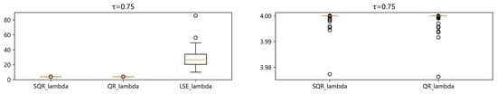
Figure 2.
Boxplot comparison of the estimated values of drift parameter .
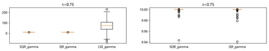
Figure 3.
Boxplot comparison of the estimated values of drift parameter .
From the overall estimation of the drift parameters in Table 1 and Table 2, it can be seen that regardless of the quantile, the self-weighted quantile estimator and the quantile estimator significantly outperform the least squares estimator in terms of mean, standard deviation, and mean squared error. Under the premise that the true parameter values are , it can be seen from the mean indicator that the estimated values of the self-weighted quantile estimator and the quantile estimator are very close to the true values, with the best performance at the 0.75 quantile and the self-weighted quantile estimation effect being better than the quantile estimation. The estimated values of the two parameters to be estimated for the sample path are shown below, and box plots are drawn for visualization, as shown in Figure 2 and Figure 3. It can be seen that the median of the LSE estimated values is significantly different from the estimated results of SQR and QR at the 0.75 quantile. The median of the SQR and QR estimated values is very close, but the right box plot shows that the QR estimated values have more outliers.
Monte Carlo simulation results for drift parameters and via SQR method across various quantiles of weight Function (59) are displayed in Table 3 and Table 4, which show how the different choices of can influence the properties of the estimator. It is found the 0.95 quantile of weight Function (59) possesses the smaller bias and MSE.
4. Statistical Arbitrage Strategy Based on Self-Weighted Quantile Estimation of Jump O-U Process
In cross-period arbitrage trading, considering that the futures market has night trading, and for the same trading rules, overnight strategies may lead to large fluctuations in the price spread of different futures contracts at the opening of the next day when facing major policy changes or large fluctuations in the external market at night, thereby increasing the risk. Therefore, in order to avoid the adverse impact of such fluctuations on the performance of cross-period arbitrage, it is more reasonable to choose intra-day trading for cross-period arbitrage strategies, and at the same time, in order to increase potential arbitrage opportunities, high-frequency data is chosen for modeling, pursuing higher returns under low risk.
4.1. Data Sources and Descriptive Statistics
This paper selects the CSI 300 stock index futures contract of the China Financial Futures Exchange as the research object for empirical analysis, and the main terms of the contract are listed in the following Table 5.
Table 5.
China Financial Futures Exchange CSI 300 stock index futures contract.
Select the 5 min closing prices of the current month and next month contracts of the CSI 300 stock index futures as the samples for this trading strategy, with contract codes IF00 and IF01, respectively. The time span is from 12 April 2021 to 5 December 2023, with a total of 30,905 data points. Among them, the data from 12 April 2021 to 31 December 2022 is used as the in-sample data for fitting the jump O-U process and parameter estimation, and the data from 1 January 2023 to 5 December 2023 is used as the out-of-sample backtesting data to evaluate the strategy performance. The data is sourced from the Wind Financial Data Platform, and data processing is carried out using Python version 3.8 and R version 4.1.
The descriptive statistics of the 5 min high-frequency closing prices of the two contracts are as follows Table 6.
Table 6.
Descriptive statistics of CSI 300 stock index futures current month and next month contracts.
Sliced data from April 2021 is extracted to show the local trend chart of the current month and next month contracts as follows.
As shown in Figure 4, the current month and next month contracts of the CSI 300 stock index futures have a trend of rising and falling together, and there is a close correlation between the contracts. Since the variety is the same, the price trend is highly correlated and affected by similar factors. However, the simultaneous rise and fall does not necessarily mean that there is a stable correlation. It is still necessary to calculate the correlation coefficient and conduct sufficient market analysis to choose this pair of contracts for arbitrage, ensuring the stability of the statistical arbitrage strategy and reducing the strategy risk.
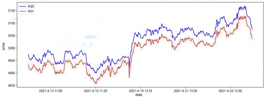
Figure 4.
The local trend of the CSI 300 stock index futures contracts for the current and next month.
4.2. Data Processing and Sample Testing
4.2.1. Correlation Test
The Pearson correlation coefficient between the two contract asset prices and the t-statistic of the Fisher correlation coefficient significance test can be calculated to determine whether they have correlation. The Pearson correlation coefficient is a statistical measure of the degree of linear correlation between two variables, with a range of −1 to 1. When the correlation coefficient is close to 1, it indicates that the two variables are positively correlated; when it is close to −1, it indicates that the two variables are negatively correlated; when it is close to 0, it indicates that there is no linear correlation between the two variables. The Fisher significance statistic is used to test whether the Pearson correlation coefficient is significantly different from 0, thereby determining whether there is a significant linear correlation between the two variables. Statistically, if the p-value of the Fisher significance statistic is less than the set significance level (usually 0.05), the original hypothesis can be rejected, that is, it is considered that there is a significant linear correlation between the two variables. The test results are as follows.
From the Table 7, it can be seen that at the 5% significance level, the original hypothesis is rejected, that is, it can be considered that there is a significant correlation between the current month and next month contracts of the CSI 300 stock index futures.
Table 7.
Correlation coefficient and significance test between IF00 and IF01.
4.2.2. Stationarity Test
Before conducting the cointegration test on the 5 min quotation time series of the current month and next month contracts of the CSI 300 stock index futures, it is first necessary to determine that these two time series have the same order of integration, so it is necessary to conduct the unit root test on the series first. In order to ensure that there is no spurious regression between the paired two contract price sequences, this paper uses Python software to conduct the ADF test on them, respectively, and judges whether the p-value is less than 0.01 at the 99% confidence level to reject the original hypothesis (that is, when the p-value is less than 0.01, the original hypothesis is rejected). If the original hypothesis is not rejected, the corresponding sequence is differenced and the above process is repeated until a stationary sequence is tested. The test results are shown in the following Table 8.
Table 8.
ADF unit root test results.
In Table 8, the test form c indicates that the test equation has an intercept term, t indicates the existence of a trend term, and k indicates the lag order. The ADF values of the price sequences and their first differences of CSI 300 IF00 futures contract and CSI 300 IF01 futures contract per hand are calculated, respectively. The test results show that at the 1%, 5%, and 10% significance levels, the absolute values of the ADF values of IF00 and IF01 are less than the absolute values of the critical values, so the original hypothesis is accepted, and it is considered that they are non-stationary sequences. Therefore, further test the stationarity of the difference sequences . The test results show that at the 1%, 5%, and 10% significance levels, the absolute values of the ADF values of the difference sequences are greater than the absolute values of the critical values, and the original hypothesis is rejected, and it is considered that the price difference sequences of CSI 300 IF00 futures contract and CSI 300 IF01 futures contract per hand are stationary sequences. Therefore, the price time sequences of CSI 300 IF00 futures contract and CSI 300 IF01 futures contract per hand are all first-order integrated, that is, they are processes.
4.3. Cointegration Test
Futures price sequences are generally non-stationary time series, but there may be a long-term equilibrium relationship between futures with high correlation. In order to effectively measure this relationship, Engle and Granger proposed the concept of cointegration. If the price sequences of two futures themselves are not stationary, but become stationary after differencing, then it is very necessary to determine the long-term equilibrium relationship between futures through cointegration test. Through the ADF unit root test, we concluded that the price sequences of the current month and next month contracts of the CSI 300 stock index futures are all first-order integrated, so the Engle–Granger two-step method can be used for testing. First, estimate the cointegration regression equation with the least squares method to obtain the following cointegration relationship:
where the coefficient 1.0140 is the weight for buying and selling contracts during backtesting, that is the , indicating that for every 1 hand of IF00 contract bought, the corresponding 1.0140 hands of IF01 contract are sold. The goodness of fit is 0.99939.
Secondly, test whether the residual term is stationary. Based on the ADF test, the ADF value is −3.85414, its absolute value is greater than the absolute values of each critical value; the p-value is 0.00239, less than 0.05, rejecting the original hypothesis, it can be considered that there is a long-term equilibrium relationship between IF00 and IF01, and the next step of verification and testing can be carried out.
4.3.1. Descriptive Statistics of Spread Sequence
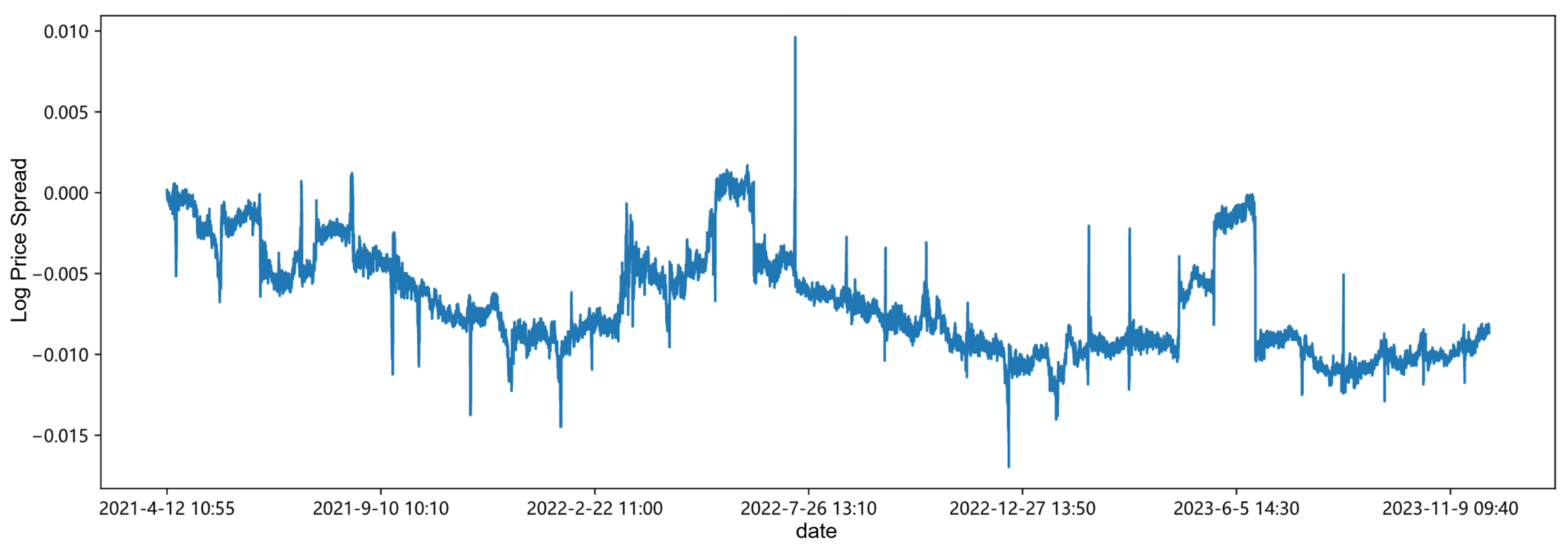
After the above tests, we define the spread of the paired futures contracts. Assuming that the price sequences of the current month contract A and the next month contract B of the CSI 300 stock index futures are and , respectively, then the spread sequence is expressed as
Its overall trend is shown in Figure 5.
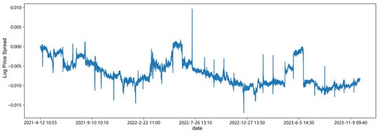
Figure 5.
Overall trend of spread sequence.
Descriptive statistics were performed on the spread sequence, and the results are as follows.
From Table 9, it can be seen that the standard deviation of the data is large, indicating a high degree of dispersion. The skewness and kurtosis indicate that the data distribution is roughly symmetrical, slightly skewed to the left, and slightly flatter relative to the normal distribution. The p-value is the p-value of the ADF stationarity test, less than 0.05, indicating that the spread sequence has stationarity.
Table 9.
Descriptive statistics of spread sequence.
4.3.2. Jump Test
Since this paper uses the jump O-U process to fit and estimate the spread sequence, compared with the ordinary O-U process, this process adds a jump term to describe the phenomenon of large fluctuations in prices in a short time, better capturing extreme fluctuations or non-mean properties in the market. Therefore, we use the LM test proposed by Lee and Mykland [49] to test the data for jumps point-by-point and calculate the amplitude of the jumps. The jump amplitude is visualized and plotted as shown in Figure 6.
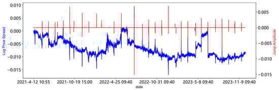
Figure 6.
Jump detection of spread sequence.
4.4. Design of Statistical Arbitrage Strategy Scheme
4.4.1. Trading Rule Settings
In a statistical arbitrage strategy, screening targets and strategy timing are both very important key factors, which have a decisive effect on whether the strategy has good performance. In the strategy scheme design of this paper, we do not screen targets through a target pool, but test the targets that have been seen well, and use the self-weighted quantile estimation results of this paper to conduct technical analysis for strategy timing, determine when to make buying and selling decisions, and reasonably set the trigger levels of trading signals.
In the traditional cointegration timing strategy, the standard deviation multiple method is usually used for timing, that is, for the spread sequence of paired targets, calculate its historical equilibrium level and standard deviation, and determine whether to open or close positions according to the multiple of the spread sequence exceeding or less than the historical equilibrium level. However, such a threshold set relying on a simple multiple for timing may miss many potential profitable trading opportunities. For example, a high threshold leads to too few trades, reducing the total statistical arbitrage profit, while a low threshold may lead to frequent trading, and the high transaction costs will erode a lot of profit and may even lead to losses, and cannot obtain the statistical arbitrage returns brought by deviations. Therefore, this paper uses the target of maximizing the expected return per unit time, calculates the probability distribution and density function of the average duration of a trading cycle, and uses the opening and closing trading points obtained for trading.
The opening and closing trading rules are shown in Table 10. When the spread sequence crosses down through the lower trigger point a, buy 1 contract of the current month and sell times the next month’s contract, where is the cointegration coefficient of the two contracts. If is not an integer, round it to the nearest whole number. When the spread sequence crosses up through the mean line, close the position. When the spread sequence crosses up through the upper trigger point m, open a position to sell 1 contract of the current month and buy times the next month’s contract. When the spread sequence crosses down through the mean line, reverse close the position. This trading rule aims to ensure the market neutrality of the investment portfolio, enabling the portfolio to achieve the expected return regardless of whether the future market trend is upward or downward.
Table 10.
Trading rules for opening and closing positions.
During the arbitrage process, the next opening position can only be triggered after the spread sequence is closed; otherwise, the original position is held until it is closed. Secondly, rolling over positions from one contract month to the next is a common operation in futures trading. As the contract expiration date approaches, investors close their futures positions and open new futures positions in the next expiration month to avoid the risks and costs associated with actual delivery, while extending the holding period of their positions. However, this paper does not perform rolling operations, i.e., it closes positions on the contract expiration date and does not open positions for the next month of the same contract after delivery. Finally, the cost settings for strategic simulated trading are as follows: the opening and closing fees are six ten-thousandths, without calculating the costs of price impact and slippage. The initial capital is set at one unit, and the returns for each time point are calculated using the rate of return. The weight ratio for buying and selling contracts is set through the cointegration coefficient.
4.4.2. Parameter Estimation and Trading Signal Determination
Within the backtesting framework, the dataset is initially segmented with 2023 as the pivot point. The dataset from 2021 to 2022 is primarily used for fitting and parameter estimation, while the 2023 dataset is used for out-of-sample simulation trading and backtesting to calculate strategy returns and other metrics. Subsequently, during the backtesting period, we dynamically estimate and adjust the calculations for parameter estimation and trading signals. By promptly incorporating the sample data from the previous time point into the historical spread sequence, we obtain the historical spread sequence closest to the point to be estimated. Parameter estimation is conducted based on this spread sequence, and the different parameter estimates at each time point are used to calculate the trading signal thresholds by substituting into Equations (11) and (13). As out-of-sample data is continuously updated and added, our strategy can better adapt to price changes.
To achieve the optimal result, we employed a grid search approach to determine the optimal quantile levels for calculating the lower and upper thresholds, a and m, using the self-weighted method. Specifically, we evaluated quantile levels in increments of 0.25 and computed the corresponding threshold values. An arbitrage strategy was then executed based on trading signals generated when the spread exceeded these thresholds.
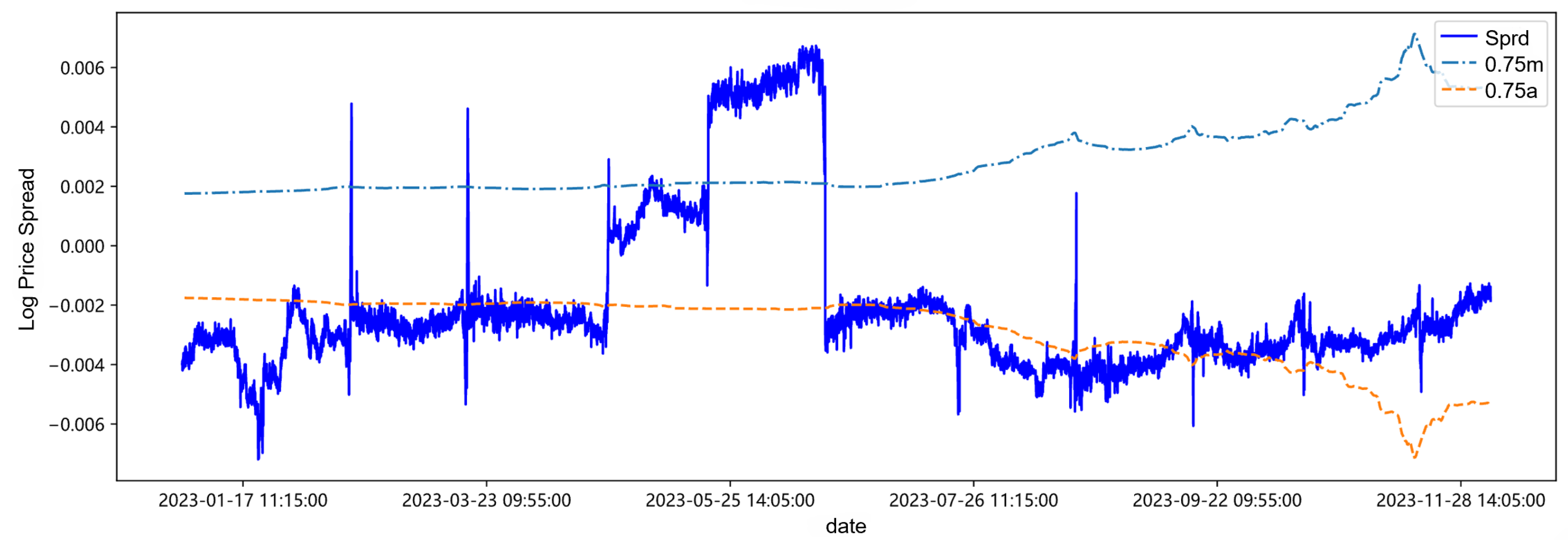
After establishing the trading rules, fitting estimation, and trading signal calculations, we select the self-weighted quantile estimation results at the 0.25, 0.75, and 0.9 quantiles to observe whether there are any patterns in the trading trigger threshold lines obtained based on different quantile estimates, whether they have a significant impact on strategy returns, and whether layered investment strategies based on different quantiles can be developed. The parameter estimation results and thresholds for the 0.75 quantile are shown in Table 11, and the trading thresholds for each quantile are visualized in Figure 7, Figure 8, Figure 9, Figure 10 and Figure 11.
Table 11.
Time series data example.
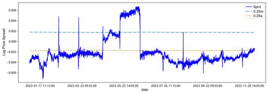
Figure 7.
Trading threshold at 0.25 quantile.
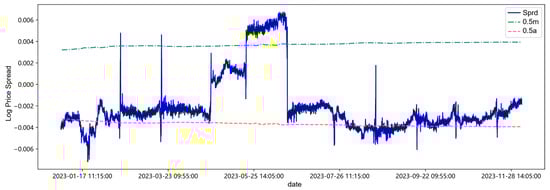
Figure 8.
Trading threshold at 0.5 quantile.

Figure 9.
Trading threshold at 0.75 quantile.
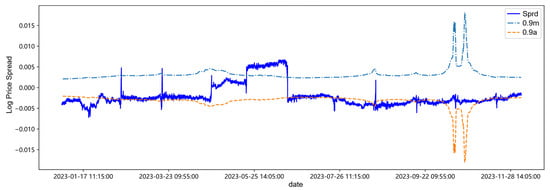
Figure 10.
Trading threshold at 0.9 quantile.
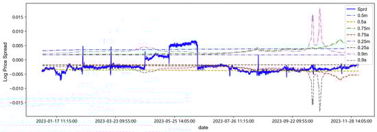
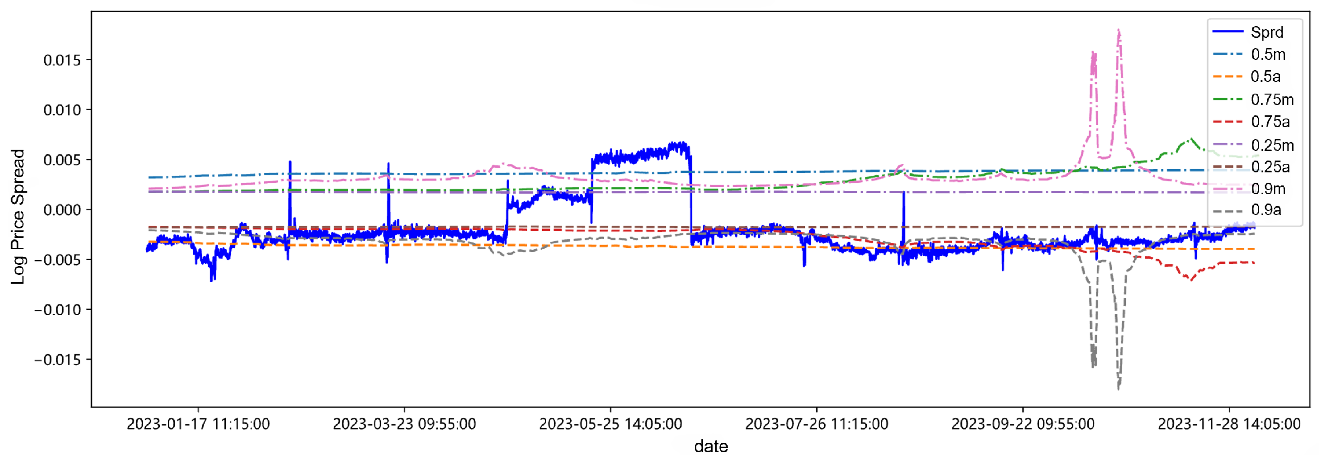
Figure 11.
Trading thresholds at various quantiles.
After centering the spread sequence, the mean is 0, the upper trigger threshold line is m, and the lower trigger threshold line is a. Observing and analyzing in combination with Table 11 and Figure 11, first of all, it can be found in Table 11 and Figure 11 that with the continuous addition of the latest out-of-sample data in the backtesting process, the parameter estimation values and trading thresholds change accordingly. Secondly, at low quantiles such as 0.25 quantile and 0.5 quantile, the changes in the threshold lines are small, while with the increase of the quantile, it may be affected by the sudden change of the spread from April to June in 2023. The sudden increase of the spread in this period leads to an increase in the amount of high quantile data, changing the data structure of the high quantile, causing the corresponding changes in the volatility and drift parameters, and thus the fluctuation of the threshold line increases. Finally, from the overall spread sequence, the threshold lines of each quantile have little impact on the triggering of trading time points, which may be attributed to the data structure distribution of the target.
4.4.3. Arbitrage Strategy Return Statistics and Indicator Assessment
Based on the trading rules outlined in Section 4.4.1, we perform a backtesting analysis of the pair trading strategy. To evaluate profitability, we use metrics total return rate and annualized return, while annualized volatility and the Sharpe ratio are employed to assess the associated risk. The results of the strategy implemented at each quantile are shown in the following Table 12.
Table 12.
Strategy return statistics at different quantiles.
As the simulation trading progresses, by the end of the strategy, there are a total of 5 trading cycles and 20 buy/sell transactions. During 2023, the strategy returns are positive at all quantiles, but the return rate and Sharpe ratio are not high. On one hand, this is due to the limited number of transactions, and on the other hand, we did not set a stop-loss line, which led to the consumption of previous gains during the long holding period. The strategy’s net value curve is shown in Figure 12. It can be observed that the strategy at the 0.5 quantile has the highest net value, and regardless of the quantile, the overall net value of the strategy shows a step-like upward trend, with some drawdowns at a few points and intervals. This is partly because the trading decisions triggered are not 100% correct, and partly due to the long-term holding without a stop-loss line, which consumes the gains.
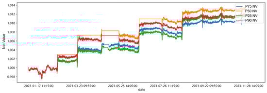
Figure 12.
Net value of statistical arbitrage strategy in backtesting period.
As shown in Table 12, the annualized volatility is relatively high, but the drawdowns in the net value curve of Figure 12 are not significant. It can be judged that the strategy has a relatively high risk compared to the return, but the drawdown risk is controllable. This indicates that by increasing the number of transactions or setting a stop-loss line, the strategy’s returns can be increased, thereby improving the overall Sharpe ratio of the strategy to a more desirable level.
Next, we compare the performance of pair trading strategies triggered by thresholds derived from self-weighted quantile estimation and the variance multiplier method. The variance multiplier approach serves as a benchmark due to its widespread use in practice. Given that the residuals from the regression between the prices of two paired equities follow a normal distribution, the variance multiplier is commonly used to determine trading thresholds. To adapt to changing market conditions, we implement a rolling window approach, re-estimating the variance at each window and dynamically adjusting the thresholds for the pair trading strategy. The rolling window length is set to match that of the self-weighted quantile estimation to ensure consistency in threshold updates. The performance of the variance multiplier-based strategy is reported in Table 13.
Table 13.
Strategy return statistics at different variance multipliers.
In terms of return performance, the self-weighted quantile estimation method significantly outperforms the variance multiplier-based strategy. The former achieves total return rates between 1.056% and 1.310%, whereas the latter yields a maximum of only 0.003%. Similarly, the annualized return rate for the self-weighted quantile approach remains consistently higher (0.025% to 0.031%) compared to the variance-based strategy, which produces returns on the order of %. These results indicate that self-weighted quantile estimation is far more effective in generating cumulative and annualized returns, making it a superior choice for return maximization.
On the risk side, the self-weighted quantile estimation strategy exhibits an annualized volatility range of 0.184% to 0.228%, significantly higher than the near-zero volatility observed in the variance multiplier-based approach. While the lower volatility in the latter suggests greater stability, it may also indicate overly conservative risk constraints, which limit return potential. The Sharpe ratio comparison further highlights this contrast: the self-weighted quantile estimation method achieves Sharpe ratios between 0.111 and 0.167, whereas the variance-based strategy reaches a maximum of just 0.052. Given that a higher Sharpe ratio signifies better risk-adjusted returns, the self-weighted quantile estimation method emerges as the more attractive option, offering a better balance between risk and return.
5. Conclusions
On the theoretical front, this paper introduces self-weighted quantile estimation into the estimation of the drift parameters of the jump Ornstein–Uhlenbeck process, and proves the asymptotic normality of the estimator under large sample properties in a statistical sense. At the same time, through Monte Carlo simulation experiments, it verifies that compared to other estimators under this stochastic process, the self-weighted quantile estimator has better stability and accuracy in estimation performance.
In the empirical part, this paper first verifies the existence of jumps in asset prices (spreads) in the financial market, detects the direction and magnitude of asset price jumps through the LM test, and then matches them with the jump Ornstein–Uhlenbeck process, proving that the stochastic process with a jump term can better fit the jumps and other phenomena existing in the actual financial market. Secondly, under the premise of being as close as possible to the real market rules, this paper studies the statistical arbitrage strategy under the high-frequency data of CSI 300 stock index futures, conducts multiple tests on the related asset price sequences, sets reasonable trading trigger thresholds based on the goal of maximizing the expected return per unit time of the trading cycle, and conducts strategy backtesting at multiple quantiles. The backtesting results prove that the jump Ornstein–Uhlenbeck process and self-weighted quantile method adopted in this paper perform well in empirical tests. In the out-of-sample backtesting period of 2023, the number of trading cycles for each strategy is 5, and all quantiles have achieved positive returns, with an average total return rate of 1.17%. Thirdly, the net value curves of the strategies at each quantile are similar, all showing a step-like upward trend, with no obvious drawdowns, and the highest net value at the 0.5 quantile. Finally, due to the limited number of trading times and the absence of a stop-loss line, the annualized return rate of the strategy is relatively low compared to the annualized volatility, resulting in a lower Sharpe ratio, but the drawdown risk is controllable. This indicates that by adjusting the number of trades and setting a stop-loss line, the returns can be increased to some extent, thereby improving the Sharpe ratio and achieving a more desirable level.
However, due to the focus and depth of our research, this paper has certain limitations and potential directions for future study. As this paper focuses on methodology rather than practical implementation, our empirical study does not take into account factors such as capital constraints and liquidity issues in high-frequency pair trading, even though they are crucial to trading performance. We plan to explore these aspects further in future research.
Author Contributions
Conceptualization, Y.S.; methodology, Y.S.; software, C.C.; validation, R.C.; formal analysis, C.C.; investigation, Y.Z.; resources, M.Z.; data curation, C.C.; writing—original draft preparation, R.C.; writing—review and editing, M.Z.; visualization, Y.Z.; supervision, M.Z.; project administration, Y.S.; funding acquisition, Y.S. All authors have read and agreed to the published version of the manuscript.
Funding
This research work is supported by National Natural Science Foundation of China (11901397).
Data Availability Statement
The dataset for the empirical analysis can be derived from the following resource available in the public domain: https://www.joinquant.com/data/ (accessed on 1 January 2024).
Conflicts of Interest
The authors declare no conflicts of interest.
References
- Griffin, J.E.; Steel, M.F. Inference with non-Gaussian Ornstein–Uhlenbeck processes for stochastic volatility. J. Econom. 2006, 134, 605–644. [Google Scholar] [CrossRef]
- Roberts, G.O.; Papaspiliopoulos, O.; Dellaportas, P. Bayesian inference for non-Gaussian Ornstein–Uhlenbeck stochastic volatility processes. J. R. Stat. Soc. Ser. B Stat. Methodol. 2004, 66, 369–393. [Google Scholar] [CrossRef]
- Jongbloed, G.; Van Der Meulen, F.H.; Van Der Vaart, A.W. Nonparametric inference for Lévy-driven Ornstein-Uhlenbeck processes. Bernoulli 2005, 11, 759–791. [Google Scholar] [CrossRef]
- Valdivieso, L. Parameter estimation for an IG-OU stochastic volatility model. Math. Day 2005, 95. [Google Scholar]
- Valdivieso, L.; Schoutens, W.; Tuerlinckx, F. Maximum likelihood estimation in processes of Ornstein-Uhlenbeck type. Stat. Inference Stoch. Process. 2009, 12, 1–19. [Google Scholar] [CrossRef]
- Barndorff-Nielsen, O.E.; Shephard, N. Non-Gaussian Ornstein–Uhlenbeck-based models and some of their uses in financial economics. J. R. Stat. Soc. Ser. B (Stat. Methodol.) 2001, 63, 167–241. [Google Scholar] [CrossRef]
- Jongbloed, G.; Van Der Meulen, F.H. Parametric estimation for subordinators and induced OU processes. Scand. J. Stat. 2006, 33, 825–847. [Google Scholar] [CrossRef]
- Zhang, S.; Zhang, X.; Sun, S. Parametric estimation of discretely sampled Gamma-OU processes. Sci. China Ser. A Math. 2006, 49, 1231–1257. [Google Scholar] [CrossRef]
- Brockwell, P.J.; Davis, R.A.; Yang, Y. Estimation for nonnegative Lévy-driven Ornstein-Uhlenbeck processes. J. Appl. Probab. 2007, 44, 977–989. [Google Scholar] [CrossRef]
- Leonenko, N.; Sakhno, L.; Šuvak, N. Parameter estimation for reciprocal gamma Ornstein–Uhlenbeck type processes. Theory Probab. Math. Stat. 2013, 86, 137–154. [Google Scholar] [CrossRef]
- Zhang, S.; Zhang, X. Moment estimation of parameters for discretely sampled OU-compound Poisson processes. Chin. J. Appl. Probab. Stat. 2010, 26, 384–398. [Google Scholar]
- Wu, Y.; Hu, J.; Zhang, X. Moment estimators for the parameters of Ornstein-Uhlenbeck processes driven by compound Poisson processes. Discret. Event Dyn. Syst. 2019, 29, 57–77. [Google Scholar] [CrossRef]
- Hu, Y.; Long, H. Least squares estimator for Ornstein–Uhlenbeck processes driven by α-stable motions. Stoch. Process. Their Appl. 2009, 119, 2465–2480. [Google Scholar] [CrossRef]
- Zhang, S.; Zhang, X. A least squares estimator for discretely observed Ornstein–Uhlenbeck processes driven by symmetric α-stable motions. Ann. Inst. Stat. Math. 2013, 65, 89–103. [Google Scholar] [CrossRef]
- Long, H. Least squares estimator for discretely observed Ornstein–Uhlenbeck processes with small Lévy noises. Stat. Probab. Lett. 2009, 79, 2076–2085. [Google Scholar] [CrossRef]
- Masuda, H. Approximate self-weighted LAD estimation of discretely observed ergodic Ornstein-Uhlenbeck processes. Electron. J. Stat. 2010, 4, 525–565. [Google Scholar] [CrossRef]
- Taufer, E.; Leonenko, N. Characteristic function estimation of non-Gaussian Ornstein–Uhlenbeck processes. J. Stat. Plan. Inference 2009, 139, 3050–3063. [Google Scholar] [CrossRef]
- Hu, Y.; Long, H. Parameter estimation for Ornstein-Uhlenbeck processes driven by α-stable Lévy motions. Commun. Stoch. Anal. 2007, 1, 1. [Google Scholar] [CrossRef]
- Mai, H. Efficient maximum likelihood estimation for Lévy-driven Ornstein–Uhlenbeck processes. Bernoulli 2014, 20, 919–957. [Google Scholar] [CrossRef]
- Spiliopoulos, K.V. Method of moments estimation of Ornstein-Uhlenbeck processes driven by general Lévy process. In Annales de l’ISUP; LSTA: Paris, France, 2009; Volume 53, pp. 3–18. [Google Scholar]
- Wu, Y.; Hu, J.; Yang, X. Moment estimators for parameters of Lévy-driven Ornstein–Uhlenbeck processes. J. Time Ser. Anal. 2022, 43, 610–639. [Google Scholar] [CrossRef]
- Shu, H.; Jiang, Z.; Zhang, X. Parameter estimation for integrated Ornstein–Uhlenbeck processes with small Lévy noises. Stat. Probab. Lett. 2023, 199, 109851. [Google Scholar] [CrossRef]
- Wang, J.; Wang, L.; Li, H. Parameter Estimation for the Harmonic Fractional Ornstein-Uhlenbeck Financial Model. J. Henan Norm. Univ. (Nat. Sci. Ed.) 2025, 53, 75–81. [Google Scholar] [CrossRef]
- Han, Y.; Hu, Y.; Zhang, D. Modified least squares estimators for Ornstein–Uhlenbeck processes from low-frequency observations. Appl. Math. Lett. 2024, 156, 109143. [Google Scholar] [CrossRef]
- Alazemi, F.; Alsenafi, A.; Chen, Y.; Zhou, H. Parameter estimation for the complex fractional Ornstein–Uhlenbeck processes with Hurst parameter H ∈ (0, 12). Chaos Solitons Fractals 2024, 188, 115556. [Google Scholar] [CrossRef]
- Zhang, D. Statistical inference for Ornstein–Uhlenbeck processes based on low-frequency observations. Stat. Probab. Lett. 2025, 216, 110286. [Google Scholar] [CrossRef]
- Sutcliffe, C.; Board, J. The Effects of Spot Transparency on Bid-Ask Spreads and Volume of Traded Share Options; University of Southampton: Southampton, UK, 1996. [Google Scholar]
- Bondarenko, O. Statistical arbitrage and securities prices. Rev. Financ. Stud. 2003, 16, 875–919. [Google Scholar] [CrossRef]
- Hogan, S.; Jarrow, R.; Teo, M.; Warachka, M. Testing market efficiency using statistical arbitrage with applications to momentum and value strategies. J. Financ. Econ. 2004, 73, 525–565. [Google Scholar] [CrossRef]
- Alexander, C.; Dimitriu, A. A comparison of cointegration and tracking error models for mutual funds and hedge funds. ISMA Cent. Discuss. Pap. Financ. 2004, 4, 1–26. [Google Scholar]
- Elliott, R.J.; Van Der Hoek, J.; Malcolm, W.P. Pairs trading. Quant. Financ. 2005, 5, 271–276. [Google Scholar] [CrossRef]
- Bertram, W.K. Analytic solutions for optimal statistical arbitrage trading. Phys. A Stat. Mech. Its Appl. 2010, 389, 2234–2243. [Google Scholar] [CrossRef]
- Rudy, J.; Dunis, C.; Giorgioni, G.; Laws, J. Statistical Arbitrage and High-Frequency Data with an Application to Eurostoxx 50 Equities. 2010. Available online: https://ssrn.com/abstract=2272605 (accessed on 1 January 2024).
- Fang, H. Empirical Research on the Theoretical Model and Application Analysis of Statistical Arbitrage Based on China’s Closed-end Fund Market. Stat. Decis. 2005, 3. [Google Scholar]
- Caldeira, J.F.; Moura, G.V. Selection of a portfolio of pairs based on cointegration: A statistical arbitrage strategy. Rev. Bras. Financ. 2013, 11, 49–80. [Google Scholar] [CrossRef]
- Zhu, L.r.; Su, X.; Zhou, Y. Research on Statistical Arbitrage Based on China’s Futures Market. J. Appl. Stat. Manag. 2015, 34, 11. [Google Scholar]
- Fan, B.T. Futures arbitrage of different varieties and based on the cointegration which is under the framework of bayesian-in the case of soy oil and palm oil. DEStech Trans. Econ. Bus. Manag. 2018. [Google Scholar] [CrossRef]
- Wang, J.; Cui, W.; Wang, C. Research on Statistical Arbitrage of Stock Index Futures Based on Time-Varying Coefficient Cointegration. Wuhan Financ. 2017, 29–33. [Google Scholar]
- Liu, Y.; Lu, Y. Empirical Study on Statistical Arbitrage of Options and Futures Based on the O-U Process. Mod. Bus. Trade Ind. 2016, 37, 2. [Google Scholar]
- Zhang, L. Application Research on the Cross-Breed Arbitrage of O-U Model in Agricultural Futures Market. Ph.D. Thesis, Anhui University, Hefei, China, 2018. [Google Scholar]
- Wu, L.; Zang, X.; Zhao, H. Analytic value function for a pairs trading strategy with a Lévy-driven Ornstein–Uhlenbeck process. Quant. Financ. 2020, 20, 1285–1306. [Google Scholar] [CrossRef]
- Sabino, P. Exact simulation of variance gamma-related ou processes: Application to the pricing of energy derivatives. Appl. Math. Financ. 2020, 27, 207–227. [Google Scholar] [CrossRef]
- Zhao, H.; Luo, P.; Wang, S. High-frequency pairs trading in Chinese stock market: Based on Lévy-OU processes. Syst. Eng.-Theory Pract. 2023, 43, 2251–2265. [Google Scholar]
- Ken-Iti, S. Lévy Processes and Infinitely Divisible Distributions; Cambridge University Press: Cambridge, UK, 1999; Volume 68. [Google Scholar]
- Masuda, H. Ergodicity and exponential β-mixing bounds for multidimensional diffusions with jumps. Stoch. Process. Their Appl. 2007, 117, 35–56. [Google Scholar] [CrossRef]
- Ling, S. Self-weighted least absolute deviation estimation for infinite variance autoregressive models. J. R. Stat. Soc. Ser. B Stat. Methodol. 2005, 67, 381–393. [Google Scholar] [CrossRef]
- Hjort, N.L.; Pollard, D. Asymptotics for minimisers of convex processes. arXiv 2011, arXiv:1107.3806. [Google Scholar]
- Knight, K. Limiting distributions for L1 regression estimators under general conditions. Ann. Stat. 1998, 26, 755–770. [Google Scholar] [CrossRef]
- Lee, S.S.; Mykland, P.A. Jumps in financial markets: A new nonparametric test and jump dynamics. Rev. Financ. Stud. 2008, 21, 2535–2563. [Google Scholar] [CrossRef]


Disclaimer/Publisher’s Note: The statements, opinions and data contained in all publications are solely those of the individual author(s) and contributor(s) and not of MDPI and/or the editor(s). MDPI and/or the editor(s) disclaim responsibility for any injury to people or property resulting from any ideas, methods, instructions or products referred to in the content. |
© 2025 by the authors. Licensee MDPI, Basel, Switzerland. This article is an open access article distributed under the terms and conditions of the Creative Commons Attribution (CC BY) license (https://creativecommons.org/licenses/by/4.0/).