More Theory About Infinite Numbers and Important Applications

Abstract

In the author’s previous studies, new infinite numbers, their properties, and calculations were introduced. These infinite numbers quantify infinity and offer new possibilities for solving complicated problems in mathematics and applied sciences in which infinity appears. The current study presents additional properties and topics regarding infinite numbers, as well as a comparison between infinite numbers. In this way, complex problems with inequalities involving series of numbers, in addition to limits of functions of x $\in$ ℝ and improper integrals, can be addressed and solved easily. Furthermore, this study introduces rotational infinite numbers. These are not single numbers but sets of infinite numbers produced as the vectors of ordinary infinite numbers are rotated in the complex plane. Some properties of rotational infinite numbers and their calculations are presented. The rotational infinity unit, its inverse, and its opposite number, as well as the angular velocity of rotational infinite numbers, are defined and illustrated. Based on the above, the Riemann zeta function is equivalently written as the sum of three rotational infinite numbers, and it is further investigated and analyzed from another point of view. Furthermore, this study reveals and proves interesting formulas relating to the Riemann zeta function that can elegantly and simply calculate complicated ratios of infinite series of numbers. Finally, the above theoretical results were verified by a computational numerical simulation, which confirms the correctness of the analytical results. In summary, rotational infinite numbers can be used to easily analyze and solve problems that are difficult or impossible to solve using other methods.

1. Introduction

As there is no record of earlier civilizations conceptualizing or discussing infinity, the history of infinity begins with the Ancient Greeks. Yet the concept of infinity was forced upon the Greeks by the physical world via three traditional observations: (i) time seems endless, (ii) space and time can be unendingly subdivided, and (iii) space is without bounds. Aristotle thought being infinite was a privation, not perfection; it was the absence of a limit. Archimedes derived the formula for the area of a circle by thinking of a circle as a polygon with infinitely many infinitesimal sides.

The Greek philosopher and mathematician Zeno of Elea (~450 BC) tried to show the “physical” impossibility of infinity, not by measuring it but by using it to divide things into smaller and smaller elements. The result is his famous “arrow paradox” in which, according to him, an arrow should never be able to hit its target. Indeed, one can always divide the arrow’s remaining path by two, and a portion of the path will always remain untravelled (1/2, 1/4, 1/8, 1/16, 1/32, …), ad infinitum. Since it takes an infinite number of steps to cross the distance between the bow and the target, Zeno concluded that it was impossible for the arrow to reach its destination in a finite time. However, this paradox was solved much later by one of the branches of mathematics that studies infinite sums of numbers: the series. Adding 1/2 + 1/4 + 1/8 + 1/16 + … is like adding 1/2 + 1/2² + 1/2³ + 1/2⁴ + … + 1/2ⁿ+… This type of series is called a geometric series. Its resolution is very simple: when n tends to infinity, the value of this sum tends to one [1].

As European mathematicians struggled with the foundation of calculus in the 17th century, it remained unclear whether infinity could be considered a number or magnitude and, if so, how this could be achieved [2]. The topic of infinitely small numbers prompted the discovery of calculus in the late 1600s by the German mathematician Gottfried Wilhelm Leibniz and the English mathematician Isaac Newton. Leibniz’s derivation of calculus extensively used “infinitesimal” numbers which were both nonzero but small enough to add to any real number without changing it noticeably.

Georg Cantor (1845 AD–1918 AD) [3] went further than anyone else by asking a simple question: Can we compare two sets of infinite numbers? Can one be “bigger” than the other? His method pairs an element of the first set with an element of the second. If each element finds its partner and none remain unpaired (a bijection), then we can say that the two sets are equal. Cantor distinguished between a particular set and the abstract concept of its size or cardinality when comparing sets. Cantor called the sizes of his infinite sets “transfinite cardinals”. Thus, the modern mathematical conception of quantitative infinity developed in the late 19th century from works by Cantor, Gottlob Frege, Richard Dedekind, and others using the idea of collections or sets [2,3,4,5,6,7].

However, in 1960, Abraham Robinson developed nonstandard analysis, in which the reals are rigorously extended to include infinitesimal numbers and infinite numbers; this new extended field is called the field of hyperreal numbers. The goal was to create a system of analysis that was more intuitively appealing than standard analysis but without losing the rigor of standard analysis. According to him, the theory of infinitesimals was eventually replaced by the classical theory of limits [8,9,10,11,12,13,14]. In nonstandard analysis, infinitesimals are invertible, and their inverses are infinite numbers. These infinities are part of a hyperreal field; there is no equivalence between them, as with Cantorian transfinites. For example, if H is an infinite number in this sense, then H + H = 2H and H + 1 are distinct infinite numbers. This method of nonstandard calculus was fully developed by Keisler (1986) [11].

Unlike previous attempts to quantify infinity, by applying the theory of limits of functions, new infinite numbers and functions were defined as limits of complex functions tending to infinity in the author’s previous papers [15,16,17]. The fundamental definitions, lemmas, theorems, and properties concerning these new infinite numbers and functions, as well as illustrative mathematical and engineering applications, were presented and proven. The new infinite numbers retain important properties of real/complex numbers (arithmetic operations, powers, roots, etc.). The set of infinite numbers is a superset of the complex numbers set. These new infinite numbers quantify infinity (in a way that is different than past efforts) and are a useful tool for solving problems where infinity appears. Using these numbers and functions, the extended (in infinite numbers) Laplace and bilateral Laplace transforms, also proposed in [15,17], make it possible to solve specific differential equations defined piecewise over the entire domain of real numbers (−∞, +∞). Moreover, by using the infinite number functions, long series of infinite terms can be nicely transformed into short, elegant infinite number functions whose computation is an easy task. Additionally, a simple, efficient criterion for series convergence was developed. Furthermore, by calculating and using the derivatives/integrals of these infinite number functions, complicated limits of series of numbers, as well as ratios of the form ∞/∞, can be easily calculated in cases where L’Hôpital’s rule cannot be applied.

In the present study, more properties of infinite numbers are presented and used. The arguments of infinite numbers, briefly mentioned in the author’s previous papers, are also presented and further discussed. These arguments (measure, angle, and velocity) will be useful in the complex plane vector representation of infinite numbers and rotational infinite numbers, as well as in comparing infinite numbers. A criterion for the comparison of the measures of infinite numbers is presented. Moreover, a similar criterion is described specifically for infinite numbers whose functions are real (not complex). In addition, a lemma on comparing infinite numbers using a comparison of their velocities is illustrated and proven. In this way, complex problems with inequalities involving series of numbers, limits of functions of x $\in$ ℝ, and improper integrals can be easily solved. Furthermore, rotational infinite numbers are introduced; these are generated as the vectors of ordinary infinite numbers are rotated in the complex plane. The rotational infinity unit and its velocity are defined, and their representation in the complex plane is illustrated. Moreover, the angular velocity (ω) of rotational infinite numbers is presented, which is much simpler than velocity (v), indicating a much more perceptible concept: the speed of rotation. In addition, the Riemann zeta function ζ(s) is described using infinite numbers. It is proved that ζ(s) can be written as the sum of three rotational infinite numbers, all rotating with a similar angular velocity, which have as their sum a finite number and not infinity. Furthermore, interesting formulas concerning the Riemann zeta function are proved, which help to solve complex mathematical problems with series of numbers. Finally, the study proceeds to numerical simulation for the computational examination and validation of the results, where it is indeed verified that the approximately calculated numerical results perfectly approximate the analytical ones. In conclusion, based on the above, the presented ordinary/rotational infinite numbers, with their properties, can easily solve problems that are quite difficult or impossible to solve using conventional methods. Such problems, for example, include those described below by relations (11), (76), (81), (82), (86), and (87).

The rest of this study is organized as follows: Section 2 presents and illustrates some introductory concepts and definitions, such as the velocity of infinite numbers and their comparison. Section 3 deals with introducing new rotational infinite numbers, and more specifically, the rotational infinity unit, its opposite and inverse numbers, the definition of rotational infinite functions and numbers, their vector representation, their angular velocity, and some topics with opposite rotational infinite numbers. In Section 4, the Riemann zeta function is written equivalently using rotational infinite numbers. It is also depicted in the complex plane via vector representation, and, in addition, interesting formulas are revealed and proven, which are useful in solving problems with ratios of complicated series of numbers. Section 5 presents some computational simulation results. In Section 6, the conclusions of this study are presented.

Table 1. Summary of notation.

Symbol	Description
ξ	The infinity unit
φ(ξ), f(ξ) or A(ξ)	An infinite number function
φ’(ξ) or {d/dξ [φ(ξ)]}	First derivative of infinite number function φ(ξ)
A	The set of all infinite numbers
|φ(ξ)|	Measure or absolute value of an infinite number φ(ξ)
θ	Angle of an infinite number
v	Velocity of an infinite number
Ru	The rotational infinity unit
A(ξ)eiφ(ξ)	A rotational infinite number
ω	Angular velocity of a rotational infinite number
ζ(s)	Riemann zeta function
s	A complex variable equal to α + ib, where α, b real numbers

provides a short summary of the notation used in this article.

2. Introductory Concepts

As shown in [15,17], by definition, the relation (1) gives the infinity unit, ξ. Moreover, every single-value, continuous, differentiable, and non-oscillating complex function, φ(.), of the infinity unit, ξ, namely, the function φ(ξ), is an “infinite number function”, which is also an “infinite number”. Considering relation (1) and the fact that φ(.) is a continuous function, the infinite number φ(ξ) is the limit of a complex function given by formula (2). Consequently, φ(ξ) can be infinity, a finite number, or zero.

The set of all these numbers is the set of infinite numbers and is denoted by the capital letter A (in bold). In contrast to infinity in its general consideration (∞), where no arithmetic operations apply (e.g., ∞−∞ = undefined, ∞/∞ = undefined, etc.), arithmetic operations are possible for infinite numbers (e.g., ξ−ξ = 0, ξ/ξ = 1, and 3ξ/ξ = 3, etc.), given that (ξ) no longer represents infinity in its general determination but its specific univocal form, which is the infinity unit (ξ) defined by Equation (1). Arithmetic operations on infinite numbers are performed just like arithmetic operations on limits of functions, since infinite numbers are limits of functions.

$$\xi \equiv \underset{x\to +\infty }{\lim }(x) \mathrm{where} x\in ℝ$$

(1)

$$\varphi (\xi )=\varphi (\underset{x\to +\infty }{\lim }x)=\underset{x\to +\infty }{\lim }\varphi (x)$$

(2)

Example 1. 

$${\displaystyle \frac{{\xi }^2-4{\xi }^2}{7\xi -\xi }}\cdot \ln ({\xi }^2)=\underset{x\to +\infty }{\lim }\left({\displaystyle \frac{x^2-4x^2}{7x-x}}\cdot \ln (x^2)\right)=\underset{x\to +\infty }{\lim }\left(-x\cdot \ln (x)\right)=-\underset{x\to +\infty }{\lim }x\cdot \ln (\underset{x\to +\infty }{\lim }x)=-\xi \ln \xi$$

2.1. Arguments of Infinite Numbers

In this section, the three arguments of infinite numbers are presented and further analyzed. These arguments include the “measure”, the “angle”, and the “velocity”, which will be useful in the complex plane vector representation of infinite numbers and rotational infinite numbers, as well as in the comparison of infinite numbers (as we will see below).

The “measure” or “absolute value”, |φ(ξ)|, of an infinite number φ(ξ), written in the form $\varphi (\xi )=f_1(\xi )+i{f}_2(\xi )$, where f₁(.) and f₂(.) are single-value, continuous, differentiable, and non-oscillating real functions, is defined by Formula (3). Furthermore, by combining Formulas (1) and (3), relationship (4) applies.

$$|\varphi (\xi )|=\sqrt{f_1{}^2(\xi )+f_2{}^2(\xi )}$$

(3)

$$|\varphi (\xi )|=\underset{x\to +\infty }{\lim }\sqrt{f_1{}^2(x)+f_2{}^2(x)} \mathrm{where}\mathrm{x}\in ℝ$$

(4)

Example 2. 

Based on Formula (3), it is calculated that

$$\begin{gathered} for {\varphi }_1(\xi )=\xi +i\sqrt{2\xi +1} \Rightarrow \left|{\varphi }_1(\xi )\right|=\sqrt{{\xi }^2+2\xi +1}=\sqrt{{(\xi +1)}^2}=\xi +1 \\ for {\varphi }_2(\xi )=-i{\displaystyle \frac{2}{3}}\xi \Rightarrow \left|{\varphi }_2(\xi )\right|={\displaystyle \frac{2}{3}}\xi \end{gathered}$$

The “angle”, (θ), of an infinite number φ(ξ) written in the form $\varphi (\xi )=f_1(\xi )+i{f}_2(\xi )$, where f₁(.) and f₂(.) are single-value, continuous, differentiable, and non-oscillating real functions, is defined with respect to the positive half-axis of the real numbers of the complex plane according to Formula (5).

$$\theta =\arctan \left({\displaystyle \frac{f_2(\xi )}{f_1(\xi )}}\right)$$

(5)

Example 3. 

Based on Formula (5), it is calculated that

$$for {\varphi }_1(\xi )=\xi +i\xi \Rightarrow {\theta }_1=\arctan \left({\displaystyle \frac{\xi }{\xi }}\right)=\arctan \left(1\right)={45}^0$$

Definition 1. 

The “velocity”, (v), of an infinite number φ(ξ) written in the form, $\varphi (\xi )=f_1(\xi )+i{f}_2(\xi )$, where f₁(.) and f₂(.) are single-value, continuous, differentiable, and non-oscillating real functions, is defined as its first derivative $d\varphi (\xi )/d\xi$, given by Formula (6).

$$v={\displaystyle \frac{d\varphi (\xi )}{d\xi }}=\varphi ’(\xi )={\displaystyle \frac{d}{d\xi }}\left(f_1(\xi )+i{f}_2(\xi )\right)={\displaystyle \frac{d{f}_1(\xi )}{d\xi }}+i{\displaystyle \frac{d{f}_2(\xi )}{d\xi }}$$

(6)

Using relation (1) and given that f₁(.) and f₂(.) are continuous functions, Equation (6) is equivalently transformed:

$$v=\underset{x\to +\infty }{\lim }{\displaystyle \frac{d{f}_1(x)}{dx}}+i\underset{x\to +\infty }{\lim }{\displaystyle \frac{d{f}_2(x)}{dx}} \mathrm{where}\mathrm{x}\in ℝ$$

Example 4. 

• The following examples concern infinite numbers φ(ξ) whose function φ(.) is a real function.

  $$\begin{array}{c}for {\varphi }_1(\xi )=\xi \Rightarrow v_1={\displaystyle \frac{d\xi }{d\xi }}=1, for {\varphi }_2(\xi )={\xi }^2 \Rightarrow v_2={\displaystyle \frac{d{\xi }^2}{d\xi }}=2\xi \hfill \\ for {\varphi }_3(\xi )=-0.5\xi \Rightarrow v_3= {\displaystyle \frac{d(-0.5\xi )}{d\xi }}=-0.5, for {\varphi }_4(\xi )=\ln (\xi ) \Rightarrow v_4={\displaystyle \frac{d(\ln \xi )}{d\xi }}={\displaystyle \frac{1}{\xi }}\hfill \end{array}$$

Therefore, various velocities are observed above whose absolute values range from a zero value (1/ξ) that has the infinite number φ₄(ξ) = lnξ, and it is the smallest possible velocity (in absolute values) up to infinite velocity values, e.g., with the function φ₂(ξ) = ξ². Among all these, the function φ₁(ξ) = ξ, that is, the infinity unit function, has a unitary velocity (v₁ = 1).

• On the other hand, the following example concerns an infinite number φ(ξ) whose function φ(.) is complex.
  For $\varphi (\xi )=3{\xi }^2+\xi \ln (3)+\ln (2{\xi }^2)+i \xi \sqrt{\xi }$, we have a velocity equal to$\left(6\xi +\ln (3)+{\displaystyle \frac{2}{\xi }}\right)+i {\displaystyle \frac{3\sqrt{\xi }}{2}}$and whose measure is equal to$\sqrt{{\left(6\xi +\ln (3)+{\displaystyle \frac{2}{\xi }}\right)}^2+ {\left({\displaystyle \frac{3\sqrt{\xi }}{2}}\right)}^2}=\sqrt{36{\xi }^2+\left(12\ln (3)+{\displaystyle \frac{9}{4}}\right)\xi +24+{(\ln 3)}^2+{\displaystyle \frac{4\ln (3)}{\xi }}+{\displaystyle \frac{4}{{\xi }^2}}}$.

Remark 1. 

The velocity of an infinite number φ(ξ) shows how fast the corresponding complex function $\varphi (x)=f_1(x)+i{f}_2(x)$ tends to infinity when x→∞. If this function φ(.) does not tend to infinity, e.g., the constant function φ(ξ) = c, where c $\in$ ℂ, then the velocity is, of course, zero.

2.2. Infinite Numbers Vector Representation in the Complex Plane

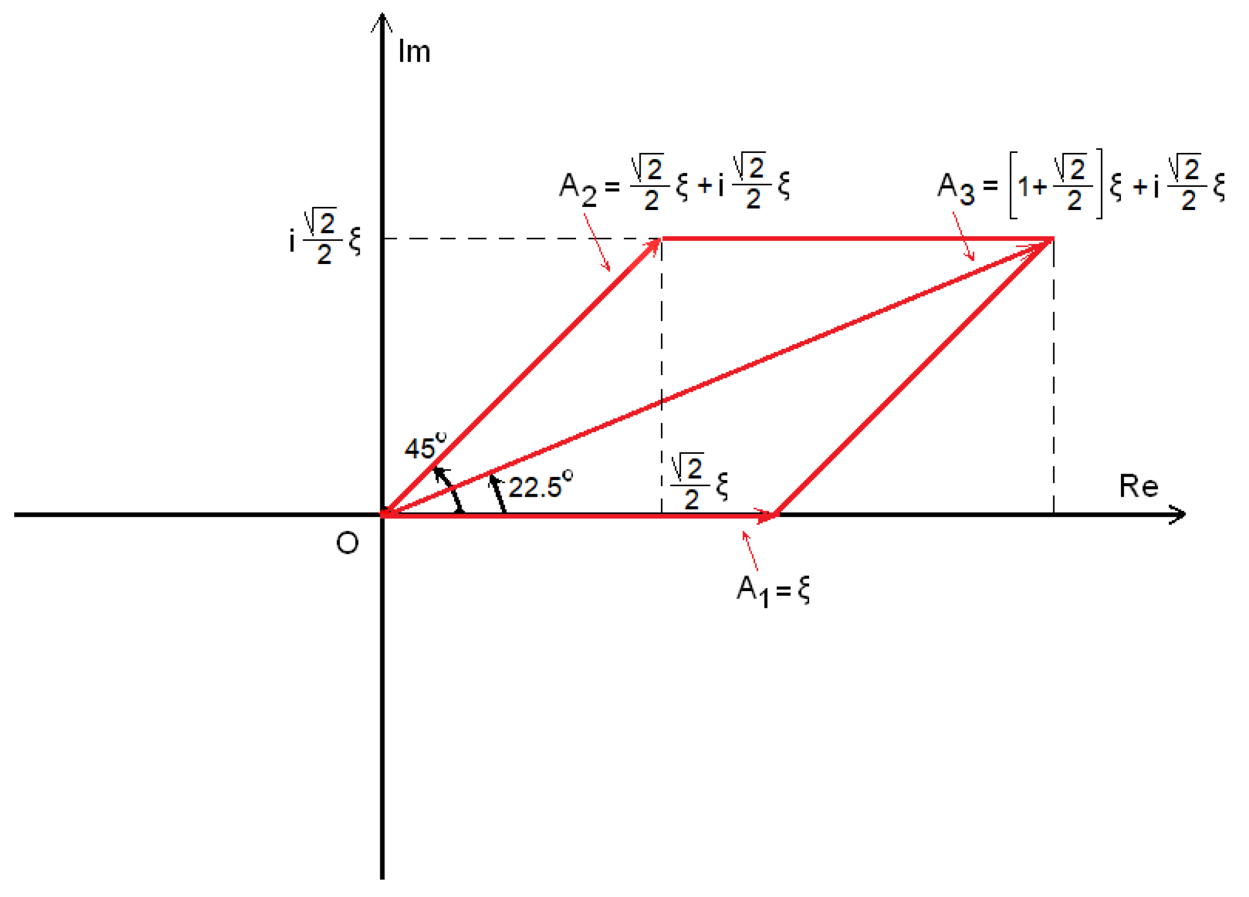
Following the above and [15,16,17], an infinite number, A = φ(ξ), can be represented in the complex plane by a vector whose length is equal to the measure (absolute value), |φ(ξ)|, and its angle with respect to the positive half-axis of the real numbers is equal to the angle, θ, of that infinite number. For example, the infinite number A₁ = ξ is represented in the complex plane of Figure 1 with an infinite length vector, whose measure is $\sqrt{{\xi }^2+0^2}=\xi$ and which has an angle with respect to the positive real half-axis equal to $\theta =\arctan {\displaystyle \frac{0}{\mathsf{\xi }}}=\arctan \left(0\right)=0^0$; namely, this vector lies on the positive half-axis of the real numbers. Similarly, the infinite number $A_2={\displaystyle \frac{\sqrt{2}}{2}}\xi +i{\displaystyle \frac{\sqrt{2}}{2}}\xi$ is depicted in the complex plane by a vector whose measure is $\sqrt{{\displaystyle \frac{2}{4}}{\xi }^2+{\displaystyle \frac{2}{4}}{\xi }^2}=\xi$ and whose angle is $\theta =\arctan {\displaystyle \frac{\frac{\sqrt{2}}{2}\xi }{\frac{\sqrt{2}}{2}\xi }}=\arctan (1)={45}^0$. Thus, as can be seen in Figure 1, infinite numbers A₁ and A₂ have the same measure, $\xi$; however, they have different angles (0° and 45°, respectively).

The sum of these two infinite numbers, A₃ = A₁ + A₂, which, of course, equals $A_3=\left[1+{\displaystyle \frac{\sqrt{2}}{2}}\right]\xi +i{\displaystyle \frac{\sqrt{2}}{2}}\xi$, is indeed the vector sum of A₁ plus A₂ in the complex plane, whose angle is equal to 22.5°.

2.3. Comparison of Infinite Numbers

Definition 2. 

The infinite number, φ₁(ξ), is greater than the infinite number, φ₂(ξ) (provided that both functions φ₁(.) and φ₂(.) are real functions), when the following relation (7) holds. Moreover, for φ₁(.) and φ₂(.) to be complex functions, the measure of the infinite number ${\varphi }_1(\xi )=f_{1,1}(\xi )+i{f}_{1,2}(\xi )$ is greater than the measure of the infinite number${\varphi }_2(\xi )=f_{2,1}(\xi )+i{f}_{2,2}(\xi )$, when relation (8) holds.

$$\underset{t\to +\infty }{\lim }\left({\varphi }_1(t)-{\varphi }_2(t)\right)>0 \mathrm{where} \mathrm{t}\in ℝ$$

(7)

$$\underset{t\to +\infty }{\lim }\left(\left|f_{1,1}(t)+i{f}_{1,2}(t)\right| -\left|f_{2,1}(t)+i{f}_{2,2}(t)\right| \right)>0 \mathrm{where} \mathrm{t}\in ℝ$$

(8)

Example 5.

It holds that ${\xi }^2>2\xi$ given that $\underset{t\to +\infty }{\lim }\left(t^2-2t\right)=\underset{t\to +\infty }{\lim }{t}^2\left(1-{\displaystyle \frac{2}{t}}\right)=\underset{t\to +\infty }{\lim }{t}^2>0$.

Additionally, $\left|3\xi +i4\xi \right|<\left|i6\xi \right|$ , given that$\xi \sqrt{3^2+4^2}<6\xi \iff 5<6$

Lemma 1. 

If the velocity $v_1={\varphi }_1^{\prime }(\xi )>0$ of an infinite number φ₁(ξ), which represents plus infinity, is greater than the velocity $v_2={\varphi }_2^{\prime }(\xi )>0$ of another infinite number φ₂(ξ), which also represents plus infinity, where φ₁(.) and φ₂(.) are single-value, continuous, differentiable and non-oscillating real functions, then the infinite number φ₁(ξ) is greater than the infinite number φ₂(ξ).

Proof. 

According to L’Hôpital’s rule for infinite numbers [17], the following relation holds, so long as the ratio G is finite, +∞, −∞.

$${\displaystyle \frac{{\varphi }_1(\xi )}{{\varphi }_2(\xi )}}={\displaystyle \frac{{\varphi }_1^{\prime }(\xi )}{{\varphi }_2^{\prime }(\xi )}}={\displaystyle \frac{v_1}{v_2}}=G \mathrm{where} \mathrm{G} \mathrm{is} \mathrm{finite}, +\infty , -\infty$$

Therefore, based on the above relation, and given that φ₁(ξ), φ₂(ξ), v₁, and v₂ are all positive numbers, it holds that

$$if v_1>v_2 \Rightarrow {\varphi }_1(\xi )>{\varphi }_2(\xi )$$

(9)

□

Example 6. 

We can find values α$\in {\mathbb{R}}^{+}$ for which expression (10) is positive, where n$\in \mathbb{N}$ and x, t $\in \mathbb{R}$.

$$\underset{n\to +\infty }{\lim }\left({\displaystyle \frac{1}{1\cdot a+e}}+{\displaystyle \frac{2}{2\cdot a+e}}+\dots + {\displaystyle \frac{n}{n\cdot a+e}}\right)-\underset{x\to +\infty }{\lim }{\displaystyle \frac{2x}{a}}+\underset{x\to +\infty }{\lim }{\displaystyle \frac{e}{a^2}}\ln (ax+e)-\underset{x\to +\infty }{\lim }\alpha x+\underset{t\to \infty }{\lim }{\displaystyle \underset{x=1}{\overset{t}{\int }}\left(4-\frac{1}{x}\right)}dx$$

(10)

Proof. 

Equivalently, inequality (11) should hold:

$$\underset{n\to +\infty }{\lim }\left({\displaystyle \frac{1}{1\cdot a+e}}+{\displaystyle \frac{2}{2\cdot a+e}}+\dots + {\displaystyle \frac{n}{n\cdot a+e}}\right)-\underset{x\to +\infty }{\lim }{\displaystyle \frac{2x}{a}}+\underset{x\to +\infty }{\lim }{\displaystyle \frac{e}{a^2}}\ln (ax+e)-\underset{x\to +\infty }{\lim }\alpha x+\underset{t\to \infty }{\lim }{\displaystyle \underset{x=1}{\overset{t}{\int }}\left(4-\frac{1}{x}\right)}dx>0$$

(11)

We notice that the above expression is an addition/subtraction of five parts (limits), each of which is infinity. Moreover, these five parts are of different forms (a series of numbers, limits of functions of x $\in$ ℝ, and an improper integral), so calculations are difficult or impossible without infinite numbers.

Using infinite numbers, inequality (11) is equivalently written as

$$\left({\displaystyle \frac{1}{1\cdot a+e}}+{\displaystyle \frac{2}{2\cdot a+e}}+\dots + {\displaystyle \frac{\xi }{\xi \cdot a+e}}\right)-{\displaystyle \frac{2\xi }{a}}+{\displaystyle \frac{e}{a^2}}\ln (\xi a+e)-a\xi +{\left.\left(4x-\ln x\right)\right|}_{x=1}^{\xi }>0\iff$$

$$\left({\displaystyle \frac{1}{1\cdot a+e}}+{\displaystyle \frac{2}{2\cdot a+e}}+\dots + {\displaystyle \frac{\xi }{\xi \cdot a+e}}\right)>\left({\displaystyle \frac{\xi }{a}}-{\displaystyle \frac{e}{a^2}}\ln (\xi a+e)\right)+{\displaystyle \frac{\xi }{\alpha }}+\alpha \xi -\left(4\xi -\ln \xi -4\right)$$

(12)

We can now name the left-hand member of inequality (12) as φ₁(ξ) and the right-hand member of inequality (12) as φ₂(ξ).

According to [15,17], the velocity (first derivative), v₁, of an infinite number function φ₁(ξ), which represents a series, is the last infinite term of this series, namely, $v_1=\left({\displaystyle \frac{\xi }{\xi \cdot a+e}}\right)={\displaystyle \frac{1}{a}}$, which is always positive as long as a $\in$ R⁺. Moreover, series φ₁(ξ) is also positive, as it is the sum of infinite positive numbers.

Given that ${\displaystyle \int \frac{xdx}{ax+b}}={\displaystyle \frac{x}{a}}-{\displaystyle \frac{b}{a^2}}\ln (ax+b)$, where α, b, x $\in$ ℝ, and considering [15,17], it is also true in infinite numbers that ${\displaystyle \int \left(\frac{\xi }{a\xi +b}\right)}d\xi ={\displaystyle \frac{\xi }{a}}-{\displaystyle \frac{b}{a^2}}\ln (a\xi +b)$, or, equivalently,

$${\displaystyle \frac{d}{d\xi }}\left({\displaystyle \frac{\xi }{a}}-{\displaystyle \frac{b}{a^2}}\ln (a\xi +b)\right)=\left({\displaystyle \frac{\xi }{a\xi +b}}\right)$$

(13)

Then, assuming b =e, the velocity, v₂, of the right-hand member, φ₂(ξ), of inequality (12) is calculated as follows:

$$v_2=\left({\displaystyle \frac{\xi }{\alpha \xi +e}}\right)+{\displaystyle \frac{1}{\alpha }}+\alpha -4+{\displaystyle \frac{1}{\xi }}={\displaystyle \frac{1}{\alpha }}+{\displaystyle \frac{1}{\alpha }}+a-4={\displaystyle \frac{2}{\alpha }}+a-4$$

(14)

The above calculated derivative, $v_2=\left({\displaystyle \frac{2}{\alpha }}+a-4\right)$, is positive for the following (α) values:

$$a< 2-\sqrt{2} or a> 2+\sqrt{2} \mathrm{where} \alpha >0$$

(15)

On the other hand, v₂ is negative for the (α) values:

$$2-\sqrt{2} <a< 2+\sqrt{2}$$

(16)

According to Lemma 1, for inequality (12) to hold, it is necessary to hold inequalities (15), as well as the following inequality of derivatives (shown in (17)).

$$v_1>v_{2 } \iff {\displaystyle \frac{1}{a}}>{\displaystyle \frac{2}{a}}+a-4 \iff {\displaystyle \frac{1}{\alpha }}+a-4<0$$

(17)

Hence, inequality (17) is true for (α) values:

$$2-\sqrt{3}<a< 2+\sqrt{3}$$

(18)

Consequently, combining (15) and (18), we obtain

$$2-\sqrt{3}<a <2-\sqrt{2} or 2+\sqrt{2}<a< 2+\sqrt{3}$$

(19)

Therefore, according to the above (by applying Lemma 1), inequality (11) holds for (α) values satisfying (19).

Moreover, for (α) values, satisfying inequality (16), the derivative, v₂, is negative (not zero); therefore, the continuous function, φ₂(x), tends to minus infinity when x tends to plus infinity. This means that the infinite number φ₂(ξ) is minus infinity when (α) takes values according to inequality (16). Therefore, inequality (11) holds in this case as well, since the left-hand member of (12) is positive while the right-hand member is negative.

Finally, combining (16) and (19), we obtain

$$2-\sqrt{3}<a< 2+\sqrt{3}$$

(20)

Therefore, in general, (α) should take values from the interval $(2-\sqrt{3}, 2+\sqrt{3})$ so that the initial inequality (11) holds. □

Of course, solving this problem without using infinite numbers is not an easy task.

3. Rotational Infinite Numbers and Functions

As seen previously, infinite numbers are defined as limits of single-value, continuous, differentiable, and non-oscillating complex functions. However, we can examine the number A₁ = φ(ξ) = sin(ξ), whose function sin(.) is an oscillating function.

This number is written equally as $A_1=\underset{t\to +\infty }{\lim }\sin (t)$, where t $\in$ ℝ. Assuming $t=\theta +2k\pi$ (where k $\in$ ℤ, θ $\in$ ℝ, and $0\le \theta \le 2\pi$), when k takes consecutive integer values, 1, 2, 3, …, then t will take values from 0 to 2π, plus the integer multiples of 2π. This means that A₁ will receive all values from −1 to +1 repeatedly. Therefore, this new number, A₁, does not converge to a certain value. Hence, A₁ represents not a certain number but a set of numbers with infinite members that are all real numbers of the interval [−1, 1]. Consequently, this number belongs to a new category of numbers, which, as we will see below, are called rotational infinite numbers and represent not single numbers but sets of numbers.

3.1. Rotational Infinity Unit

Definition 3. 

Equation (21) defines the rotational infinity unit, Ru.

$$Ru=e^{i\xi }$$

(21)

Using Formula (1), relation (21) transforms into

$$Ru=e^{i\underset{t\to \infty }{\lim }t}=\underset{t\to +\infty }{\lim }{e}^{it}\hspace{1em}\hspace{1em}\mathrm{where} \mathrm{t}\in \mathbb{ℝ}$$

(22)

Furthermore, using Euler’s formula, relation (22) transforms into

$$Ru=\underset{t\to \infty }{\lim }(\cos \mathrm{t}+\mathrm{i}\cdot \sin \mathrm{t})=\cos \mathsf{\xi }+\mathrm{i}\cdot \sin \mathsf{\xi }$$

(23)

Based on relation (23), the measure of rotational infinity unit (Ru) is calculated by Equation (24):

$$\left|Ru\right|=\left|\underset{t\to \infty }{\lim }(\cos t+i\sin t)\right|=\underset{t\to \infty }{\lim }1=1$$

(24)

According to the definition of Equation (5), and considering Equation (23), the angle θ of the rotational infinity unit is calculated by Equation (25), and its value is ξ, as seen in Equation (25).

$$\theta =\arctan \left({\displaystyle \frac{f_2(\xi )}{f_1(\xi )}}\right)=\arctan \left({\displaystyle \frac{\sin \xi }{\cos \xi }}\right)=\arctan \left(\tan \xi \right)=\xi$$

(25)

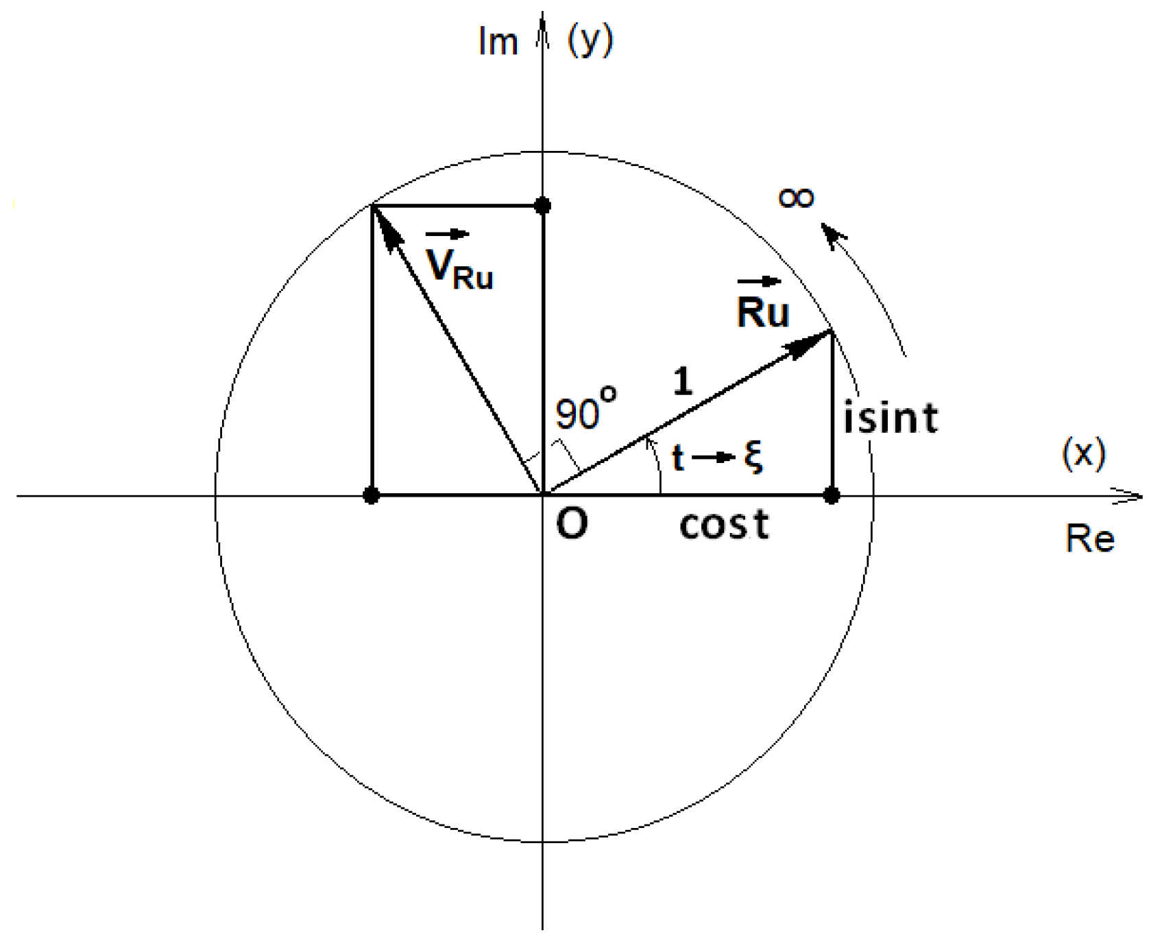
Remark 2.

Hence, the rotational infinity unit, Ru, can be depicted in the complex plane with a unit vector $\overrightarrow{Ru}$ that has an angle θ = ξ, meaning that it moves (rotates) infinitely, as shown schematically in Figure 2. Therefore, the rotational infinity unit does not receive a particular value but repeatedly receives all the complex numbers belonging to the unit circle of the complex plane. It represents a set of numbers.

3.2. Velocity of Rotational Infinity Unit

Moreover, the velocity, v_Ru, of the rotational infinity unit, Ru, is calculated by relation (26). Relationship (27) gives the measure of velocity, |v_Ru|, which equals the unit.

$$\begin{array}{cc}{v}_{Ru}={\displaystyle \frac{d(e^{i\xi })}{d\xi }}& =\underset{t\to \infty }{\lim }\left({\displaystyle \frac{d(e^{it})}{dt}}\right)=\underset{t\to \infty }{\lim }{\displaystyle \frac{d}{dt}}(\cos t+i\sin t) \mathrm{where} \mathrm{t}\in \mathbb{ℝ}\\ & =\underset{t\to \infty }{\lim }(-\sin t+i\cos t)=-\sin \xi +i\cos \xi \Rightarrow \\ & \hspace{1em}\hspace{1em}{v}_{Ru}=-\sin \xi +i\cos \xi \end{array}$$

(26)

$$\mathrm{Moreover}: \left|v_{Ru}\right|=|-\sin t+i\cos t|=1 \Rightarrow \left|v_{Ru}\right|=1$$

(27)

Finally, the angle, θ_v, of the velocity v_Ru is calculated from relation (28), and it is equal to ξ + π/2.

$${\theta }_v=\arctan \left({\displaystyle \frac{\cos \xi }{-\sin \xi }}\right)=\arctan \left({\displaystyle \frac{\sin (\xi +\pi /2)}{\cos (\xi +\pi /2)}}\right)=\arctan \left(\tan \left(\xi +{\displaystyle \frac{\pi }{2}}\right)\right)=\xi +{\displaystyle \frac{\pi }{2}}$$

(28)

Remark 3.

Therefore, the velocity v_Ru of the rotational infinity unit is also a rotational infinite number that has a unit measure and an angle advancement equal to π/2 with respect to the rotational infinity unit. Hence, the velocity v_Ru is also written as $v_{Ru}=e^{i(\xi +\pi /2)}$. Moreover, the velocity v_Ru can be depicted in the complex plane with a rotating unit vector, $\overrightarrow{v_{Ru}}$, which is perpendicular to the vector of rotational infinity unit, $\overrightarrow{Ru}$, as shown schematically in Figure 2.

Remark 4.

Consequently, in addition to the infinity unit (ξ), the number (Ru = e^iξ) is another unit, the rotational infinity unit, which denotes the rotation unit for t → ∞. Thus,

Table 2. Infinity unit vs rotational infinity unit.

	Infinity Unit (ξ)	Rotational Infinity Unit (Ru = eiξ)
Measure	ξ	1
Angle	0	ξ
Velocity measure	1	1
Velocity angle	0	ξ+π/2

applies, where the infinity unit, ξ, and the rotational infinity unit, Ru, are listed with their characteristics and compared.

3.3. Definition of Rotational Infinite Numbers and Functions

Definition 4.

“Rotational infinite functions” are defined as the functions of the infinity unit, ξ, of the form A(ξ)e^iφ(ξ), where A(ξ) and φ(ξ) are ordinary infinite numbers/functions. These “rotational infinite functions” are also “rotational infinite numbers”.

Remark 5.

Considering that the angles φ(ξ) in the above numbers are functions of ξ, these numbers are represented by vectors that rotate infinitely in the complex plane, just like the rotational infinity unit.

Remark 6.

Given Definition 4, it follows that |A(ξ)| is a measure of the rotational infinite number A(ξ)e^iφ(ξ), since Equation (29) applies. Furthermore, the angle of this rotational number is equal to φ(ξ) plus the angle of A(ξ), since Equation (30) applies.

$$\left|A(\xi )e^{i\varphi (\xi )}\right|=\left|A(\xi )\right|\cdot \left|\cos \left(\varphi (\xi )\right)+i\sin \left(\varphi (\xi )\right)\right|=\left|A(\xi )\right|$$

(29)

$$A(\xi )e^{i\varphi (\xi )}=\left|A(\xi )\right|e^{i\angle A(\xi )}{e}^{i\varphi (\xi )}=\left|A(\xi )\right|e^{i(\varphi (\xi )+\angle A(\xi ))}$$

(30)

Remark 7.

• In Definition 4, if we consider A(ξ) = 1 and φ(ξ) = ξ, we obtain the rotational infinity unit (Ru = e^iξ).
• In Definition 4, if we consider φ(ξ) = D, where D is a complex number and not a function of ξ, we obtain a non-rotating (ordinary)infinite number. For example, for A(ξ) = 3ξ + 1 and D = 2 + iπ/6, we obtain

$$(3\xi +1)e^{2+i\pi /6}=(3\xi +1)e^2{e}^{i\pi /6}=(3\xi +1)e^2(\cos {\displaystyle \frac{\pi }{6}}+i\sin {\displaystyle \frac{\pi }{6}})=(3\xi +1)e^2{\displaystyle \frac{1}{2}}+i(3\xi +1)e^2{\displaystyle \frac{\sqrt{3}}{2}}$$

As calculated by Equation (31), the above number has a constant angle, θ, equal to π/3, and is therefore not rotating.

$$\theta =\arctan \left({\displaystyle \frac{(3\xi +1)e^2\frac{\sqrt{3}}{2}}{(3\xi +1)e^2\frac{1}{2}}}\right)=\arctan \left(\sqrt{3}\right)={\displaystyle \frac{\pi }{3}}$$

(31)

Definition 5.

Two rotational infinite numbers, $A_1(\xi )e^{i{\varphi }_1(\xi )}$ and $A_2(\xi )e^{i{\varphi }_2(\xi )}$, are opposite if Equation (32) holds. Furthermore, two rotational infinite numbers, $A_1(\xi )e^{i{\varphi }_1(\xi )}$ and $A_2(\xi )e^{i{\varphi }_2(\xi )}$ are inverse if Equation (33) holds.

$$A_1(\xi )e^{i{\varphi }_1(\xi )}+A_2(\xi )e^{i{\varphi }_2(\xi )}=0$$

(32)

$$A_1(\xi )e^{i{\varphi }_1(\xi )}\cdot A_2(\xi )e^{i{\varphi }_2(\xi )}=1$$

(33)

Remark 8.

With respect to the rotational infinity unit, we have

• The opposite of the rotational infinity unit: $-e^{i\xi }=e^{i\pi }{e}^{i\xi }=e^{i(\xi +\pi )}$
• The inverse of the rotational infinity unit: ${\displaystyle \frac{1}{e^{i\xi }}}=e^{-i\xi }=e^{i(-\xi )}$

Thus, the opposite number of the rotational infinity unit, Ru, is a rotational infinite number of the same measure (equal to unit) and an angle equal to ξ + π, i.e., with an angle advancement equal to π with respect to Ru. Furthermore, the inverse of the rotational infinity unit, Ru, is a rotational infinite number of the same measure (unit) and angle, −ξ, meaning that it moves (rotates) in the inverse direction with respect to the rotational infinity unit, Ru.

Example 7.

Let us now look at some more examples of rotational infinite numbers:

• Infinite number: $e^{\xi +i\xi }$

The number $\left(e^{\xi +i\xi }\right)$ is written as $e^{\xi }\cdot e^{i\xi }$. Hence, this infinite number is of the form A(ξ)e^iφ(ξ), and therefore, it is a rotational infinite number with a measure equal to ($e^{\xi }$) and an angle equal to ξ.

The velocity of this number is

$$\begin{gathered} v={\displaystyle \frac{d}{d\xi }}(e^{\xi +i\xi })=(1+\mathrm{i})\cdot e^{\xi +i\xi }=\sqrt{2}{e}^{i\arctan {\displaystyle \frac{1}{1}}}\cdot e^{\xi +i\xi }=\sqrt{2}{e}^{\mathsf{\xi }}\cdot e^{i(\xi +\mathsf{\pi }/4)} \\ \mathrm{hence}: \left|v\right|=\sqrt{2} e^{\xi } \mathrm{and} {\theta }_v=\xi +{\displaystyle \frac{\pi }{4}} \end{gathered}$$

(34)

Thus, the number $\left(e^{\xi +i\xi }\right)$ is a rotational infinite one with the following characteristics:

(I)

Measure equal to $e^{\xi }$.

(II)

Angle θ = ξ.

(III)

Velocity measure $\left|v\right|=\sqrt{2} e^{\xi }$.

(IV)

Velocity angle θ_v = ξ + π/4, meaning an angle advancement, π/4, with respect to the initial number $\left(e^{\xi +i\xi }\right)$.

• Infinite number $(4+i3\xi )e^{i{\xi }^2}$.

The number $\left((4+i3\xi )e^{i{\xi }^2}\right)$ is written as $\sqrt{16+9{\xi }^2}\cdot e^{i\arctan {\displaystyle \frac{3\xi }{4}}}\cdot e^{i{\xi }^2}=\sqrt{16+9{\xi }^2}\cdot e^{i{\displaystyle \frac{\pi }{2}}}\cdot e^{i{\xi }^2}=\sqrt{16+9{\xi }^2}\cdot e^{i\left({\xi }^2+{\displaystyle \frac{\pi }{2}}\right)}$.

Hence, this infinite number is also a rotational one, with a measure equal to ($\sqrt{16+9{\xi }^2}\approx 3\xi$) and an angle equal to ξ² + π/2.

The velocity of this number is

$$\begin{gathered} v={\displaystyle \frac{d\left((4+i3\xi )e^{i{\xi }^2}\right)}{d\xi }}=i3e^{i{\xi }^2}+i2\xi (4+i3\xi )e^{i{\xi }^2}=\left(-6{\xi }^2+i(3+8\xi )\right)\cdot e^{i{\xi }^2} \\ =\sqrt{36{\xi }^4+{(3+8\xi )}^2}\cdot e^{i\arctan {\displaystyle \frac{3+8\xi }{-6{\xi }^2}}}\cdot e^{i{\xi }^2}=\sqrt{36{\xi }^4+{(3+8\xi )}^2}\cdot e^{i0}\cdot e^{i{\xi }^2}=\sqrt{36{\xi }^4+{(3+8\xi )}^2}\cdot e^{i{\xi }^2} \\ \mathrm{hence},\left|v\right|=\sqrt{36{\xi }^4+{(3+8\xi )}^2}\mathrm{and}{\theta }_v={\xi }^2 \end{gathered}$$

(35)

Thus, the number $\left((4+i3\xi )e^{i{\xi }^2}\right)$ is a rotational infinite one with the following characteristics:

(I)

Measure equal to $\sqrt{16+9{\xi }^2}\approx 3\xi$.

(II)

Angleθ = ξ² + π/2.

(III)

Velocity measure $\left|v\right|=\sqrt{36{\xi }^4+{(3+8\xi )}^2}$.

(IV)

Velocity angle θ_v = ξ², meaning an angle advancement, −π/2, (lag) with respect to initial number $\left((4+i3\xi )e^{i{\xi }^2}\right)$.

3.4. Angular Velocity of Rotational Infinite Numbers

Definition 6.

In any rotational infinite number of the form A(ξ)e^iφ(ξ), whose angle, $\theta =\varphi (\xi )+\angle A(\xi )$, is not a finite number but a function of ξ (that is, θ(ξ)), and which corresponds to an infinitely rotating vector at the complex plane, the angular velocity, ω, is defined by relation (36).

$$\omega =\underset{x\to +\infty }{\lim }{\displaystyle \frac{d\theta }{dx}}={\displaystyle \frac{d\theta (\xi )}{d\xi }} \mathrm{where} \mathrm{x}\in \mathbb{ℝ}$$

(36)

For example, the rotational infinite number $f(\xi )=e^{6\xi +8i\xi }$ = $e^{6\xi }\cdot e^{8i\xi }$ has a measure equal to $\left|f(\xi )\right|=e^{6\xi }$ and an angle equal to θ = 8ξ; therefore, its angular velocity (ω) is determined by Equation (37):

$$\omega ={\displaystyle \frac{d\theta }{d\xi }}={\displaystyle \frac{d\left(8\xi \right)}{d\xi }}=8$$

(37)

On the other hand, the velocity (v) of this number f(ξ) is

$$v={\displaystyle \frac{df(\xi )}{d\xi }}={\displaystyle \frac{d\left(e^{6\xi +8i\xi }\right)}{d\xi }}=(6+8i)e^{6\xi +8i\xi }$$

(38)

Remark 9.

Hence, we notice that, in rotational infinite numbers, the angular velocity (ω) is much simpler than velocity (v). Moreover, angular velocity (ω) indicates a much more perceptible concept, which is the speed of rotation. On the other hand, for all non-rotational infinite numbers, ω = 0, as expected. For example, for the infinite number (2ξ + iξ), its angular velocity, ω, is calculated by Equation (39):

$$\theta =\arctan {\displaystyle \frac{\xi }{2\xi }}=0.463647\dots$$

$$\mathit{and} \mathit{therefore}, \omega ={\displaystyle \frac{d\theta }{d\xi }}={\displaystyle \frac{d(0.463647\dots )}{d\xi }}=0$$

(39)

Let us see another example:

The number ${\xi }^{\alpha +\mathrm{ib} }={\xi }^{\alpha }\cdot {\xi }^{\mathrm{ib} }={\xi }^{\alpha }\cdot e^{i(b\ln \xi )}$ is a rotational infinite number whose measure is (${\xi }^{\alpha }$), and its angle is (θ = blnξ). The angular velocity (ω) of this infinite number is given by relation (40), where x $\in$ ℝ.

$$\omega =\underset{x\to +\infty }{\lim }{\displaystyle \frac{d\theta }{dx}}=\underset{x\to +\infty }{\lim }{\displaystyle \frac{d(b\ln x)}{dx}}=b\cdot \underset{x\to +\infty }{\lim }\left({\displaystyle \frac{1}{x}}\right)={\displaystyle \frac{b}{\xi }}=0$$

(40)

Therefore, $\left({\xi }^{\alpha +\mathrm{ib} }\right)$ is a rotational infinite number, with (I) an infinite measure (${\xi }^{\alpha }$), (II) an angle (θ = $b\ln \xi$), and (III) an angular velocity $(\omega ={\displaystyle \frac{b}{\xi }})$ that tends to zero. This rotational infinite number $\left({\xi }^{\alpha +\mathrm{ib}}\right)$ can be seen below in the analysis of the Riemann zeta function.

3.5. Opposite Rotational Infinite Numbers

Theorem 1.

For two opposite rotational infinite numbers, these numbers must have the same measure and the same angular velocity (ω), while their angles should differ from each other by (2k + 1)π, where k $\in$ ℤ.

Proof. 

Let us use the following two rotational infinite numbers, $A_1=A_{11}(\xi )e^{i{\varphi }_1(\xi )}$ and $A_2=A_{21}(\xi )e^{i{\varphi }_2(\xi )}$. These numbers can be further written as follows:

$$\begin{gathered} A_1=A_{11}(\xi )e^{i{\varphi }_1(\xi )}=\left|A_{11}(\xi )\right|e^{i\angle A_{11}(\xi )}{e}^{i{\varphi }_1(\xi )}=\left|A_{11}(\xi )\right|e^{i({\varphi }_1(\xi )+\angle A_{11}(\xi ))} \\ =\left|A_{11}(\xi )\right|\left(\cos ({\varphi }_1(\xi )+\angle A_{11}(\xi )\right)+i\sin \left({\varphi }_1(\xi )+\angle A_{11}(\xi )\right) \\ {A}_2=A_{21}(\xi )e^{i{\varphi }_1(\xi )}=\left|A_{21}(\xi )\right|e^{i\angle A_{21}(\xi )}{e}^{i{\varphi }_2(\xi )}=\left|A_{21}(\xi )\right|e^{i({\varphi }_2(\xi )+\angle A_{21}(\xi ))} \\ =\left|A_{21}(\xi )\right|\left(\cos ({\varphi }_2(\xi )+\angle A_{21}(\xi )\right)+i\sin \left({\varphi }_2(\xi )+\angle A_{21}(\xi )\right) \end{gathered}$$

Based on the above and Definition 5, in order to have $A_1+A_2=0$ meaning that $A_1=-A_2$, it is necessary that relations (41) and (42) apply:

$$\left|A_{11}(\xi )\right|\cdot \sin \left({\varphi }_1(\xi )+\angle A_{11}(\xi )\right)=-\left|A_{21}(\xi )\right|\cdot \sin \left({\varphi }_2(\xi )+\angle A_{21}(\xi )\right)$$

(41)

$$\left|A_{11}(\xi )\right|\cdot \cos \left({\varphi }_1(\xi )+\angle A_{11}(\xi )\right)=-\left|A_{21}(\xi )\right|\cdot \cos \left({\varphi }_2(\xi )+\angle A_{21}(\xi )\right)$$

(42)

Relations (41) and (42) dictate the following: (I) the amplitudes |A₁₁(ξ)| and |A₂₁(ξ)| of the above trigonometric numbers should be the same, and (II) their angles should differ from each other by an angle (2k + 1)π, where k $\in$ ℤ. Therefore, relations (43) and (44) apply:

$$\left|A_{11}(\xi )\right|=\left|A_{21}(\xi )\right|$$

(43)

$${\varphi }_1(\xi )+\angle A_{11}(\xi )={\varphi }_2(\xi )+\angle A_{21}(\xi )+(2k+1)\pi \mathrm{where}k\in \mathbb{\mathbb{Z}}$$

(44)

In Equation (44), by differentiating, we also obtain relation (45):

$$\begin{gathered} {\displaystyle \frac{d}{d\xi }}\left({\varphi }_1(\xi )+\angle A_{11}(\xi )\right)={\displaystyle \frac{d}{d\xi }}\left({\varphi }_2(\xi )+\angle A_{21}(\xi )+(2k+1)\pi \right) \\ ={\displaystyle \frac{d}{d\xi }}\left(\angle A_{21}(\xi )+{\varphi }_2(\xi )\right) \Rightarrow {\omega }_1={\omega }_2 \end{gathered}$$

(45)

□

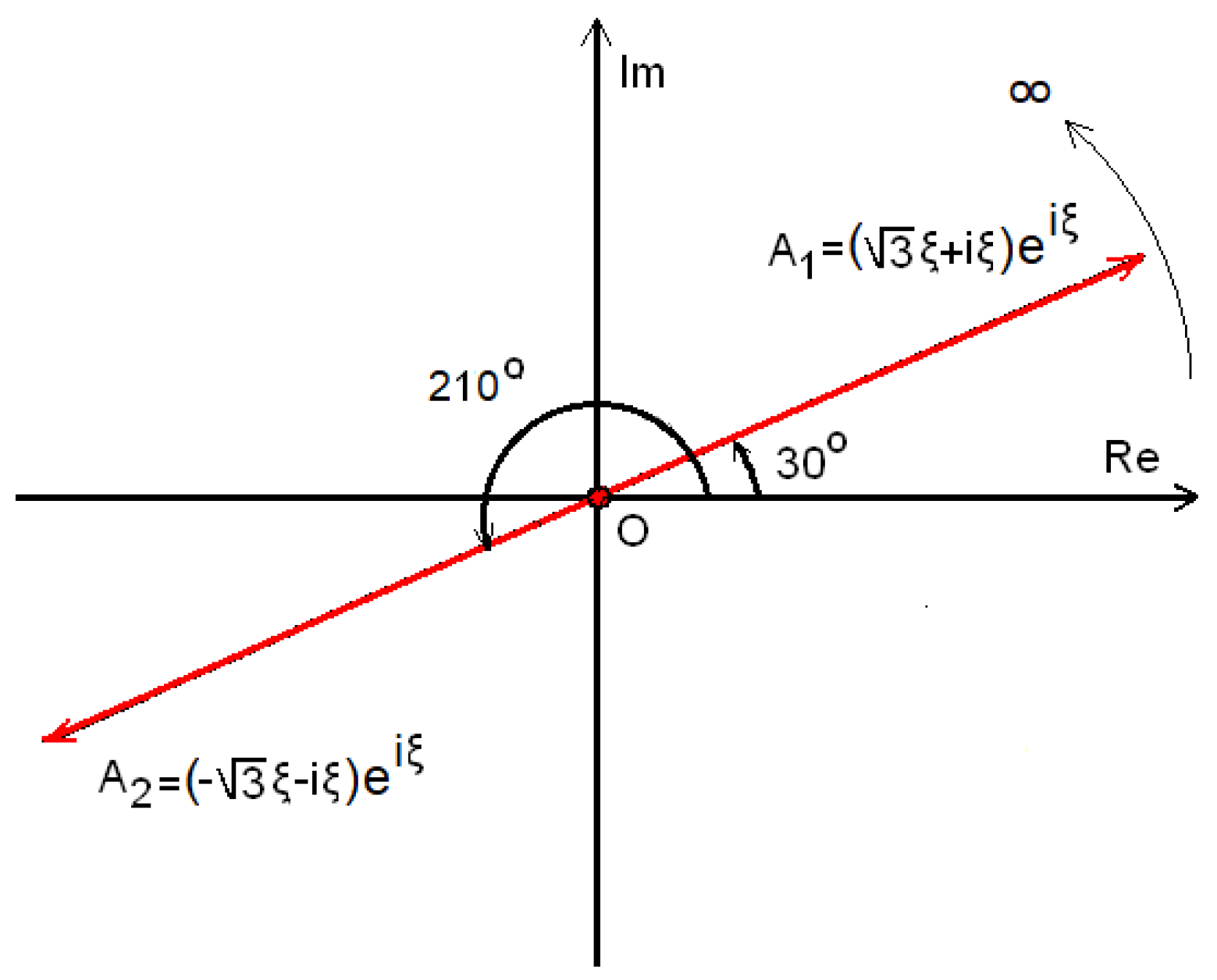
Example 8.

Figure 3 shows the two opposite rotational infinite numbers, A₁ and A₂, which are defined by relations (46) and (47).

$$A_1=(\sqrt{3}\xi +i\xi )\cdot e^{i\xi }=2\xi e^{i{\displaystyle \frac{\pi }{6}}}\cdot e^{i\xi }=2\xi e^{i(\xi +{\displaystyle \frac{\pi }{6}})}$$

(46)

$$A_2=-(\sqrt{3}\xi +i\xi )\cdot e^{i\xi }=e^{i\pi }\cdot 2\xi e^{i{\displaystyle \frac{\pi }{6}}}\cdot e^{i\xi }=2\xi e^{i(\xi +{\displaystyle \frac{7\pi }{6}})}$$

(47)

We notice that the angles of A₁ and A₂ are ($\xi +{\displaystyle \frac{\pi }{6}}$) and ($\xi +{\displaystyle \frac{7\pi }{6}}$), respectively. This means that the angular velocity of A₁ is ${\omega }_1={\displaystyle \frac{d(\xi +\pi /6)}{d\xi }}=1$ and the angular velocity of A₂ is ${\omega }_2={\displaystyle \frac{d(\xi +7\pi /6)}{d\xi }}=1$.

Consequently, the two infinite numbers, A₁ and A₂, have the same measure equal to $2\xi$ (as shown by Equations (46) and (47)). Further, they have the same angular velocity, equal to one, but they have angles that differ from each other by π (i.e., ($\xi +{\displaystyle \frac{\pi }{6}}$) and ($\xi +{\displaystyle \frac{7\pi }{6}}$), respectively).

Therefore, according to Theorem 1, the following applies:

$$A_1+A_2=0$$

On the other hand, if the infinite numberA₂ had an angle of ($2\xi +{\displaystyle \frac{7\pi }{6}}$), it would imply that its angular velocity would be equal to ${\omega }_2={\displaystyle \frac{d(2\xi +7\pi /6)}{d\xi }}=2$, which would be twice as much as the angular velocity of A₁. In this case, the sum (A₁ + A₂) would be calculated from relation (48) and, of course, would be different from zero.

$$\begin{gathered} A_1+A_2=2\xi \cdot e^{i(\xi +{\displaystyle \frac{\pi }{6}})}+2\cdot e^{i(2\xi +{\displaystyle \frac{7\pi }{6}})} \\ =2\xi \cdot e^{i{\displaystyle \frac{\pi }{6}}}\cdot e^{i\xi }+2\xi \cdot e^{i{\displaystyle \frac{7\pi }{6}}}\cdot e^{i2\xi } \\ =(\sqrt{3}\xi +i\xi )\cdot e^{i\xi }-(\sqrt{3}\xi +i\xi )\cdot e^{i2\xi } \\ =\sqrt{3}\xi \cdot e^{i\xi }+i\xi \cdot e^{i\xi }-\sqrt{3}\xi \cdot e^{i2\xi }-i\xi \cdot e^{i2\xi } \\ =\sqrt{3}\xi \cdot (\cos \xi +i\sin \xi )+i\xi \cdot (\cos \xi +i\sin \xi ) \\ -\sqrt{3}\xi \cdot (\cos 2\xi +i\sin 2\xi )-i\xi \cdot (\cos 2\xi +i\sin 2\xi ) \\ =(\sqrt{3}\cos \xi -\sin \xi -\sqrt{3}\cos 2\xi +\sin 2\xi )\cdot \xi +i(\sqrt{3}\sin \xi +\cos \xi -\sqrt{3}\sin 2\xi -\cos 2\xi )\xi \end{gathered}$$

(48)

In the same way, for any other angular velocity ω₂, so thatω₂ ≠ ω₁, we have a sum A₁ + A₂ ≠ 0.

Remark 10.

The above results also apply to three (or more) rotational infinite numbers. In particular, to have a sum equal to zero, they must have the same angular velocity, ω, which means they all rotate at the same speed. This is easily proven if we sum the first two numbers and compare them with the third.

3.6. Main Differences and Similarities Between Ordinary and Rotational Infinite Numbers

Table 3. Differences/similarities between ordinary and rotational infinite numbers.

	Ordinary Infinite Numbers	Rotational Infinite Numbers
Unit	ξ	Ru = eiξ
Mathematical notation	A(ξ)	A(ξ)eiφ(ξ)
Main difference	They are single numbers that can be real numbers or complex numbers or infinity	They are sets of ordinary infinite numbers
Arithmetic operations	Apply	Also apply
Representation in the complex plane	They are represented by constant vectors	They are represented by rotating vectors
Angular velocity (ω)	It is zero (they do not rotate)	It is a finite (not zero) real number or an infinite number
Velocity (v)	It can be zero when they are finite complex numbers	It cannot be zero since they are rotating

highlights the differences between ordinary infinite numbers and rotational infinite numbers. The rotational infinite numbers were created by the need to express and investigate the numbers resulting from the general function A(ξ)e^iφ(ξ), since this function, due to its complex power, includes sines and cosines and therefore leads to fluctuating values. Therefore, as presented in the previous analysis, these numbers constitute a different category of numbers that also possess the properties of arithmetic operations like ordinary infinite numbers.

4. Investigation of the Riemann Zeta Function Using Infinite Numbers

4.1. The Riemann Hypothesis

The Riemann hypothesis was formulated by Bernard Riemann in 1859 and has remained unresolved for over 160 years [18,19,20,21,22,23,24,25,26,27,28,29,30,31,32,33,34,35,36,37,38,39,40,41,42,43,44,45,46,47]. Today, it is considered perhaps the most important open problem in mathematics, mainly due to its close relationship with the theory of prime numbers and applications in physics, probability theory, and applied statistics. The Riemann hypothesis deals with the zeros (roots) of the Riemann zeta function and their distribution in the complex plane. In the present paper, using the rotational infinite numbers developed above, the Riemann zeta function is analyzed.

The Riemann zeta function ζ(s), given by relation (50), is an analytical continuation of the function ζ^*(s) shown in Equation (49) (where s = α + ib and α, b, x $\in$ ℝ) for values of the variable α = Re (s) > 0. Therefore, the function ζ(s) is analytical, so it is not infinity for values of α in the interval (0, 1), where, as is known, the function of Equation (49) becomes infinity. In addition, for values of the variable α in the interval (1, ∞), it also applies that ζ(s) = ζ^*(s), meaning that ζ(s) receives values identical to ζ^*(s).

$${\zeta }^{*}(s)={\displaystyle \sum _{\mathrm{n}=1}^{\infty }\frac{1}{{\mathrm{n}}^{\mathrm{s}}}}=1^{-s}+2^{-s}+3^{-s}+4^{-s}+\dots$$

(49)

Here, s = α +ib, (α, b $\in$ ℝ and α >1).

$$\zeta (\mathrm{s})={\displaystyle \frac{\mathrm{s}}{\mathrm{s}-1}}-s{\displaystyle \underset{x=1}{\overset{x=\infty }{\int }}\frac{x-⌊x⌋}{x^{s+1}}}dx$$

(50)

Here, $⌊x⌋$ is the integer part of x and α = Re(s) > 0.

The Riemann hypothesis states that all non-trivial zeros of the Riemann zeta function ζ(s) have a real part equal to one half (1/2), i.e., Re (s) = 0.5. In other words, all non-trivial zeros of the function ζ (s) lie on the critical line s = 0.5 + ib (where b $\in$ ℝ) in the complex plane. Of course, the trivial zeros of the Riemann zeta function are −2, −4, −6, …, which are easily calculated.

4.2. Description of the Riemann Zeta Function Using Rotational Infinite Numbers

Theorem 2.

The Riemann zeta function expressed by the relation $\zeta (\mathrm{s})={\displaystyle \frac{\mathrm{s}}{\mathrm{s}-1}}-s{\displaystyle \underset{x=1}{\overset{\infty }{\int }}\frac{x-⌊x⌋}{x^{s+1}}}dx$ (where s = α + ib and α, b, x $\in$ ℝ), for values 0 < α = Re(s) < 1, can be written as a sum of three rotational infinite numbers (all representing infinity), the sum of which is a finite number C.

Proof. 

The Riemann zeta function ζ(s) is further transformed, as shown below:

$$\zeta (\mathrm{s})={\displaystyle \frac{\mathrm{s}}{\mathrm{s}-1}}-s{\displaystyle \underset{x=1}{\overset{\infty }{\int }}\frac{x}{x^{s+1}}}dx+s{\displaystyle \underset{x=1}{\overset{\infty }{\int }}\frac{⌊x⌋}{x^{s+1}}}dx={\displaystyle \frac{\mathrm{s}}{\mathrm{s}-1}}-sL+sM$$

(51)

where

$$L={\displaystyle \underset{x=1}{\overset{\infty }{\int }}\frac{x}{x^{s+1}}}dx$$

(52)

and

$$M={\displaystyle \underset{x=1}{\overset{\infty }{\int }}\frac{⌊x⌋}{x^{s+1}}}dx={\displaystyle \underset{x=1}{\overset{x=2}{\int }}\frac{1}{x^{s+1}}}dx+{\displaystyle \underset{x=2}{\overset{x=3}{\int }}\frac{2}{x^{s+1}}}dx+{\displaystyle \underset{x=3}{\overset{x=4}{\int }}\frac{3}{x^{s+1}}}dx+\dots$$

(53)

Now, relation (52) is further transformed as follows:

$$L=\underset{t\to +\infty }{\lim }{\displaystyle \underset{x=1}{\overset{x=t}{\int }}\frac{x}{x^{s+1}}}dx={\displaystyle \underset{x=1}{\overset{\xi }{\int }}\frac{1}{x^s}}dx={{\displaystyle \left.\frac{1}{-s+1}{x}^{-s+1}\right|}}_{x=1}^{x=\xi }={\displaystyle \frac{1}{1-s}}\left({\xi }^{-\mathrm{s}+1}-1\right)$$

(54)

It is noted that in the above relation (54), the principal value of the multi-valued function, $1^{-\mathrm{s}+1}=1$, is obtained.

Hence, the following applies:

$$-sL={\displaystyle \frac{s}{s-1}}\cdot \left({\xi }^{-\mathrm{s}+1}-1\right)$$

(55)

Relation (53) is further transformed as follows:

$$\begin{gathered} M={\displaystyle \underset{x=1}{\overset{\infty }{\int }}\frac{⌊x⌋}{x^{s+1}}}dx={\displaystyle \underset{x=1}{\overset{x=2}{\int }}\frac{1}{x^{s+1}}}dx+{\displaystyle \underset{x=2}{\overset{x=3}{\int }}\frac{2}{x^{s+1}}}dx+\dots +{\displaystyle \underset{x=n}{\overset{x=n+1}{\int }}\frac{n}{x^{s+1}}}dx+\dots \\ ={\displaystyle \frac{1}{-s}}{\left.x^{-s}\right|}_{x=1}^{x=2}+{\displaystyle \frac{2}{-s}}{\left.x^{-s}\right|}_{x=2}^{x=3}+\dots +{\displaystyle \frac{n}{-s}}{\left.x^{-s}\right|}_{x=n}^{x=n+1}+\dots \\ ={\displaystyle \frac{1}{-s}}\left[{\left.x^{-s}\right|}_{x=1}^{x=2}+2{\left.x^{-s}\right|}_{x=2}^{x=3}+\dots +n{\left.x^{-s}\right|}_{x=n}^{x=n+1}+\dots \right] \\ ={\displaystyle \frac{1}{-s}}\left[{\left.x^{-s}\right|}_{x=1}^{x=2}+2{\left.x^{-s}\right|}_{x=2}^{x=3}+\dots +\xi {\left.x^{-s}\right|}_{x=\xi }^{x=\xi +1}\right] \\ ={\displaystyle \frac{1}{-s}}\left[2^{-s}-1^{-s}+2\cdot 3^{-s}-2\cdot 2^{-s}+\dots +\xi \cdot {(\xi +1)}^{-s}-\xi \cdot {\xi }^{-s}\right] \\ ={\displaystyle \frac{1}{-s}}\left[-1^{-s}-2^{-s}-3^{-s}-\dots -{\xi }^{-s}+\xi \cdot {(\xi +1)}^{-s}\right] \\ ={\displaystyle \frac{1}{s}}\left[1^{-s}+2^{-s}+3^{-s}+\dots +{\xi }^{-s}-\xi \cdot {(\xi +1)}^{-s}\right] \end{gathered}$$

Hence,

$$sM=\left[1^{-s}+2^{-s}+3^{-s}+\dots +{\xi }^{-s}-\xi \cdot {(\xi +1)}^{-s}\right]$$

(56)

Taking into account Equations (55) and (56), relation (51) becomes

$$\begin{gathered} \zeta (\mathrm{s})={\displaystyle \frac{\mathrm{s}}{\mathrm{s}-1}}+{\displaystyle \frac{s}{s-1}}\left({\xi }^{-\mathrm{s}+1}-1\right)+\left[1^{-s}+2^{-s}+3^{-s}+\dots +{\xi }^{-s}\right]-\xi \cdot {(\xi +1)}^{-s} \\ ={\displaystyle \frac{\mathrm{s}}{\mathrm{s}-1}}{\xi }^{-\mathrm{s}+1}+\left[1^{-s}+2^{-s}+3^{-s}+\dots +{\xi }^{-s}\right]-\xi \cdot {(\xi +1)}^{-s} \end{gathered}$$

$$\mathrm{or} \zeta (\mathrm{s})=A_1(\xi )+A_2(\xi )+A_3(\xi )$$

(57)

where

$$A_1(\xi )=A_1={\displaystyle \frac{s}{s-1}}{\xi }^{-\mathrm{s}+1}$$

(58)

$$A_2(\xi )=A_2=\left[1^{-s}+2^{-s}+3^{-s}+4^{-s}+\dots +{\xi }^{-s}\right]$$

(59)

$$A_3(\xi )=A_3=-\xi \cdot {(\xi +1)}^{-\mathrm{s}}$$

(60)

It is interesting to note that for 0 < α < 1, meaning that 0 < −α + 1 < 1, the infinite numbers A₁(ξ), A₂(ξ), and A₃(ξ) appearing in relation (57) are all infinity (Equations (58)–(60)). In particular:

• A₁(ξ): Indeed, for 0 < −α +1 < 1, the number ${\xi }^{-\mathsf{\alpha }+1}=\underset{x\to +\infty }{\lim }{x}^{-\mathsf{\alpha }+1}$ is infinity, while ${\displaystyle \frac{\sqrt{a^2+b^2}}{\sqrt{{\left(a-1\right)}^2+b^2}}}\ne 0$ (given that α > 0), and hence $\left|A_1(\xi )\right|=\left|{\displaystyle \frac{s}{s-1}}{\xi }^{-\mathrm{s}+1}\right|={\displaystyle \frac{\sqrt{a^2+b^2}}{\sqrt{{\left(a-1\right)}^2+b^2}}}{\xi }^{-\mathsf{\alpha }+1}$ is infinity, meaning that $A_1(\xi )={\displaystyle \frac{s}{s-1}}{\xi }^{-\mathrm{s}+1}$ is also infinity.
• A₂(ξ): As is known, for 0 < α < 1, the number $A_2(\xi )=\left[1^{-s}+2^{-s}+3^{-s}+\dots +{\xi }^{-s}\right]$ is infinity.
• A₃(ξ): Finally, $A_3(\xi )=-\xi \cdot {(\xi +1)}^{-\mathrm{s}}=-{\displaystyle \frac{\xi }{{(\xi +1)}^{\mathrm{s}}}}=-{\displaystyle \frac{{\xi }^s}{{(\xi +1)}^{\mathrm{s}}}}\cdot {\displaystyle \frac{\xi }{{\xi }^s}}=-{\left({\displaystyle \frac{\xi }{\xi +1}}\right)}^s\cdot {\xi }^{1-s}$

  $$=-{\left({\displaystyle \frac{1}{1+\raisebox{1ex}{$1$}\!\left/ \!\raisebox{-1ex}{$\xi $}\right.}}\right)}^s\cdot {\xi }^{1-s}=-{\xi }^{-s+1}$$

  (61)

Thus, from relation (61), it follows that A₃(ξ) is also infinite.

Considering Equations (58), (59) and (61), relation (57) becomes Equation (62). However, for 0 < α < 1, the function ζ(s) is an analytic function, which means that these three infinite numbers, (A₁(ξ), A₂(ξ), and A₃(ξ)), should have a sum that is not infinity but a finite number.

$$\zeta (s)={\displaystyle \frac{s}{s-1}}{\xi }^{-\mathrm{s}+1}+\left[1^{-s}+2^{-s}+3^{-s}+\dots +{\xi }^{-s}\right]-{\xi }^{-s+1}$$

(62)

Using the properties of infinite numbers, let us now examine whether the above sum is indeed a finite number. According to [15,17], the derivative of the infinite number function $A_2(\xi )=\left[1^{-s}+2^{-s}+3^{-s}+\dots +{\xi }^{-s}\right]$ is its last infinite term (ξ^-s), provided that the relevant criterion (Equation (63)) applies [17]:

$${\xi }^{-s}={\displaystyle \frac{{\xi }^{-s}+{(\xi -1)}^{-s}}{2}}=\dots$$

(63)

In fact, if we multiply and divide the right member of Equation (63) by (ξ^-s), we obtain the following equation, which proves that Equation (63) is true; thus, the relevant criterion holds.

$${\displaystyle \frac{{\xi }^{-s}+{(\xi -1)}^{-s}}{2}}={\xi }^{-s}\cdot {\displaystyle \frac{\frac{{\xi }^{-s}}{{\xi }^{-s}}+{\left(\frac{\xi -1}{\xi }\right)}^{-s}}{2}}={\xi }^{-s}\cdot {\displaystyle \frac{1+{\left(1-\frac{1}{\xi }\right)}^{-s}}{2}}={\xi }^{-s}\cdot {\displaystyle \frac{1+1}{2}}={\xi }^{-s}$$

Therefore, by integrating (ξ^-s), we calculate A₂(ξ) again as follows:

$$A_2(\xi )={\displaystyle \int {\xi }^{-s}d\xi }={\displaystyle \frac{{\xi }^{-s+1}}{-s+1}}+C$$

(64)

If C (in relation (64)) is not a finite number (or zero), namely, C = C(ξ), then its derivative is ${\displaystyle \frac{dC(\xi )}{d\xi }}\ne 0$; hence, from Equation (64), we obtain ${\displaystyle \frac{d{A}_2(\xi )}{d\xi }}={\xi }^{-s}+{\displaystyle \frac{dC(\xi )}{d\xi }}={\displaystyle \frac{dC(\xi )}{d\xi }}\ne 0$, which is not true (inconsistency). As mentioned above, the derivative of the series A₂(ξ) is its last infinite number, that is, ${\xi }^{-s}={\displaystyle \frac{1}{{\xi }^{\alpha +\iota b}}}=0$, given that (α) is a positive number (0 < α < 1). Therefore, C should be a finite number and not infinity.

Finally, from equations (57), (58), (61), and (64), it follows that

$$\begin{gathered} \zeta (\mathrm{s})=A_1(\xi )+A_2(\xi )+A_3(\xi )={\displaystyle \frac{s}{s-1}}{\xi }^{-\mathrm{s}+1}+{\displaystyle \frac{{\xi }^{-s+1}}{-s+1}}+C-{\xi }^{-s+1} \\ ={\displaystyle \frac{s}{s-1}}{\xi }^{-\mathrm{s}+1}+{\displaystyle \frac{{\xi }^{-s+1}}{-s+1}}+C-{\displaystyle \frac{s-1}{s-1}}{\xi }^{-s+1} \\ ={\displaystyle \frac{s}{s-1}}{\xi }^{-\mathrm{s}+1}+{\displaystyle \frac{{\xi }^{-s+1}}{-s+1}}+C-{\displaystyle \frac{s}{s-1}}{\xi }^{-s+1}+{\displaystyle \frac{1}{s-1}}{\xi }^{-s+1}=C \end{gathered}$$

(65)

proving that ζ(s) = A₁(ξ) + A₂(ξ) + A₃(ξ) is not infinity but a finite number C (depending on the values of α and b). Certainly, when C becomes zero, then we have a solution (zero) of the Riemann zeta function. This result is in agreement with the fact that ζ(s) is an analytic function. □

4.3. Remarks on the Infinite Numbers A₁(ξ), A₂(ξ), and A₃(ξ)

• Let us now further examine the infinite number A₁(ξ). The number $A_1(\xi )={\displaystyle \frac{s}{s-1}}{\xi }^{-\mathrm{s}+1}$ consists of two parts (multiplication factors).

One factor is

$${\xi }^{-\mathrm{s}+1}={\xi }^{-\alpha +1-ib}={\xi }^{-\alpha +1}{\xi }^{-ib}={\xi }^{-\alpha +1}{e}^{-ib\ln \xi }={\xi }^{-\alpha +1}{e}^{i(-b\ln \xi )}$$

(66)

As seen in Section 2, this number is a rotational infinite number, which has (I) a measure equal to (${\xi }^{-\alpha +1}$), (II) an angle equal to ($-b\ln \xi$), and (III) an angular velocity $\omega ={\displaystyle \frac{d(-b\ln \xi )}{d\xi }}=-{\displaystyle \frac{b}{\xi }}=0$ that tends to zero.

The other factor is

$${\displaystyle \frac{s}{s-1}}={\displaystyle \frac{a+ib}{a-1+ib}}={\displaystyle \frac{\sqrt{a^2+b^2}}{\sqrt{{(a-1)}^2+b^2}}}\angle \left(\arctan {\displaystyle \frac{b}{a}}-\arctan {\displaystyle \frac{b}{a-1}}\right)=r\angle \mathsf{\phi }$$

where

$$r=\left|{\displaystyle \frac{s}{s-1}}\right|={\displaystyle \frac{\sqrt{a^2+b^2}}{\sqrt{{(a-1)}^2+b^2}}}$$

(67)

$$\mathrm{and} \mathsf{\phi }=\arctan {\displaystyle \frac{b}{a}}-\arctan {\displaystyle \frac{b}{a-1}}$$

(68)

Therefore, the infinite number A₁(ξ), as a multiplication product of the above two complex factors, has a measure equal to the product of their measures, that is $(r{\xi }^{-\mathsf{\alpha }+1})$, and has an angle that is the sum of individual angles $(\mathsf{\phi }-b\ln \xi )$. Hence, its angular velocity is $\omega ={\displaystyle \frac{d(\mathsf{\phi }-b\ln \xi )}{d\xi }}=-{\displaystyle \frac{b}{\xi }}=0$. Consequently, A₁(ξ) is a rotational infinite number given by the following relation (69) and whose angular velocity tends to zero.

$$A_1(\xi )={\displaystyle \frac{s}{s-1}}{\xi }^{-\mathrm{s}+1}=r\cdot {\xi }^{1-\alpha }\cdot e^{\mathrm{i}\cdot \left(-b\ln \xi +\mathsf{\phi }\right)}$$

(69)

• Let us now examine the infinite number A₂(ξ). This number is written as

  $$\begin{gathered} A_2(\xi )=1^{-s}+2^{-s}+\dots +{(\xi -1)}^{-s}+{\xi }^{-s} \\ =1^{-a-ib}+2^{-a-ib}+\dots +{(\xi -1)}^{-a-ib}+{\xi }^{-a-ib} \\ ={\displaystyle \frac{1}{1^a}}\cdot e^{-ib\ln 1}+{\displaystyle \frac{1}{2^a}}\cdot e^{-ib\ln 2}+\dots +{\displaystyle \frac{1}{{(\xi -1)}^a}}\cdot e^{-ib\ln \xi }+{\displaystyle \frac{1}{{\xi }^a}}\cdot e^{-ib\ln \xi } \end{gathered}$$

  (70)

From equation (70), it is not obvious whether the number A₂(ξ) is a rotational infinite number. However, considering the relation (64), it is further transformed below into Equation (71), where C is a finite number:

$$\begin{gathered} A_2(\xi )={\displaystyle \frac{{\xi }^{-s+1}}{-s+1}}+C=-{\displaystyle \frac{1}{s-1}}{\xi }^{-\alpha +1}\cdot e^{-ib\ln \xi }+C \\ =-q{\xi }^{-\alpha +1}{e}^{i(-b\ln \xi +\theta )}+C=q{\xi }^{-\alpha +1}{e}^{i(-b\ln \xi +\theta +\pi )}+C \end{gathered}$$

(71)

where

$$q=\left|{\displaystyle \frac{1}{s-1}}\right|={\displaystyle \frac{1}{\sqrt{{(a-1)}^2+b^2}}}$$

(72)

$$\mathrm{and} \mathsf{\theta }=-\arctan {\displaystyle \frac{b}{a-1}}$$

(73)

From Equation (71), we calculate

$$\omega ={\displaystyle \frac{d(-b\ln \xi +\theta +\pi )}{d\xi }}=-{\displaystyle \frac{b}{\xi }}=0$$

(74)

Consequently, A₂(ξ) is also a rotational infinite number (plus the finite number C) given by relation (71), and whose angular velocity (Equation (74)) is exactly the same $(-b/\xi )$ as the angular velocity of infinite number A₁(ξ).

• Finally, let us examine the infinite number A₃(ξ). According to Equation (69) we have

  $$\begin{gathered} A_3(\xi )=-{\xi }^{1-s}=-{\xi }^{-a+1-ib}=-{\xi }^{-a+1}\cdot {\xi }^{-ib} \\ =-{\xi }^{-a+1}{e}^{-ib\ln \xi }=e^{i\pi }{\xi }^{-a+1}{e}^{-ib\ln \xi }={\xi }^{-a+1}{e}^{i(\pi -ib\ln \xi )} \end{gathered}$$

  (75)

Therefore, A₃(ξ) is also a rotational infinite number with a measure equal to ${\xi }^{-a+1}$ and an angle equal to $(\pi -ib\ln \xi )$. Hence, its angular velocity is $\omega ={\displaystyle \frac{d(\mathsf{\pi }-b\ln \xi )}{d\xi }}=-{\displaystyle \frac{b}{\xi }}=0$. Thus, the angular velocity of A₃(ξ) is exactly the same as the angular velocities of the infinite numbers A₁(ξ) and A₂(ξ) (all equal to $-b/\xi =0$).

Considering Equation (65), namely ζ(s) = A₁(ξ) + A₂(ξ) + A₃(ξ) = C, it further holds that ζ(s) − C = 0, and therefore, according to Theorem 1, all three rotating infinite numbers (excluding the finite number C), whose sum is zero, should have the same angular velocity, a fact that is proven above ($\omega =-b/\xi$).

4.4. Riemann Zeta Function Representation in the Complex Plane

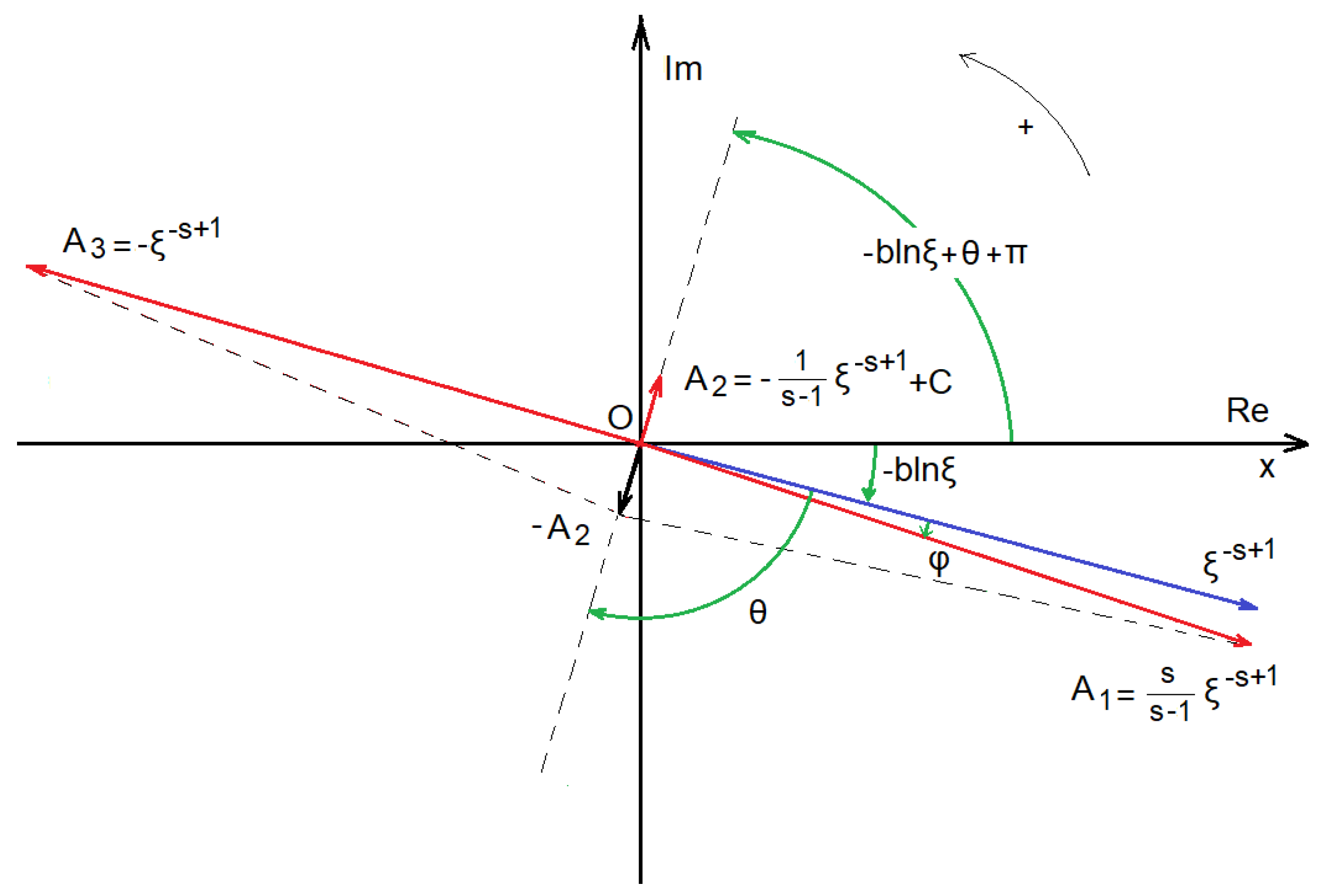
Based on the above (for values 0 <α = Re(s) < 1), we can now represent, in the complex plane, the three rotational infinite numbers A₁, A₂, and A₃, whose sum is the Riemann zeta function, ζ(s), according to Equation (57). Figure 4 schematically shows, in red, the vectors of the rotational infinite numbers A₁, A₂, and A₃ in the complex plane for random values of α and b. As seen in Figure 4, the rotational infinite number, A₁, has an angle (with respect to the Ox half axis) equal to $\angle A_1=-b\ln \xi +\mathsf{\phi }$. The rotational infinite number, A₂, has an angle $\angle A_2=-b\ln \xi +\theta +\pi$, and the rotational infinite number, A₃, has an angle $\angle A_3=\pi -b\ln \xi$. It is noted that in the scheme in Figure 4, the positive angles are all plotted anti-clockwise, and a positive, random value of the parameter b is assumed, meaning that $-b\ln \xi$, φ, and θ are all negative angles. On the other hand, the measure of A₁ is $\left|A_1\right|={\displaystyle \frac{\sqrt{a^2+b^2}}{\sqrt{{(a-1)}^2+b^2}}}\cdot {\xi }^{1-\alpha }$, the measure of A₂ is $\left|A_2\right|={\displaystyle \frac{1}{\sqrt{{(a-1)}^2+b^2}}}{\xi }^{1-\alpha }$, and the measure of A₃ is $\left|A_3\right|={\xi }^{1-\alpha }$. These three red vectors, representing the corresponding A₁, A₂, and A₃ numbers, are all rotating clockwise in the complex plane of Figure 4, with the same angular velocity $\omega =-{\displaystyle \frac{b}{\xi }}\to 0$. The sum of these three rotational infinite numbers is always a finite number C (not infinity). Of course, for the zeros (roots) of the Riemann zeta functions (i.e., suitable α and b values), we obtain C = 0, implying ζ(s) = 0, (Equation (65)). Moreover, we notice that for α =1/2, the measures of A₁ and A₃ become the same, regardless of the b values, namely,$\left|A_1\right|=\left|A_2\right|={\xi }^{1/2}=\sqrt{\xi }$, and the measure of A₂ becomes equal to $\left|A_2\right|={\displaystyle \frac{2}{\sqrt{1+4b^2}}}\sqrt{\xi }$. It is interesting to note that for higher b values, the vector of A₂ becomes increasingly smaller, while the vectors A₁ and A₃ gradually obtain an angle difference that tends to 180°, (φ→0), so that A₁ and A₃ tend to become opposite vectors.

4.5. Proof of Interesting Formulas Concerning the Riemann Zeta Function

Theorem 3.

For s₁ = a + ib₁ and s₂ = a + ib₂ and values of (a) ranging between zero and one (0 < a < 1), the following relation (76) applies.

$$\mathrm{\Lambda }={\displaystyle \frac{\left|\frac{1}{1^{s_1}}+\frac{1}{2^{s_1}}+\frac{1}{3^{s_1}}+\dots +\frac{1}{{\xi }^{s_1}}\right|}{\left|\frac{1}{1^{s_2}}+\frac{1}{2^{s_2}}+\frac{1}{3^{s_2}}+\dots +\frac{1}{{\xi }^{s_2}}\right|}}=\sqrt{{\displaystyle \frac{{(1-\alpha )}^2+b_2{}^2}{{(1-\alpha )}^2+b_1{}^2}}}$$

(76)

Proof. 

Based on Equations (59) and (64), the first member of the above relation is further transformed into Equation (77), where C1 and C2 are finite numbers.

$$\mathrm{\Lambda }={\displaystyle \frac{\left|\frac{1}{1^{s_1}}+\frac{1}{2^{s_1}}+\frac{1}{3^{s_1}}+\dots +\frac{1}{{\xi }^{s_1}}\right|}{\left|\frac{1}{1^{s_2}}+\frac{1}{2^{s_2}}+\frac{1}{3^{s_2}}+\dots +\frac{1}{{\xi }^{s_2}}\right|}}={\displaystyle \frac{\left|\frac{{\xi }^{-s_1+1}}{-s_1+1}+C1\right|}{\left|\frac{{\xi }^{-s_2+1}}{-s_2+1}+C2\right|}}$$

(77)

In addition, the following applies:

$${\xi }^{-s_1+1}={\xi }^{-\alpha +1}{e}^{-i{b}_1\ln \xi } \Rightarrow {\displaystyle \frac{{\xi }^{-s_1+1}}{{\xi }^{-\alpha +1}}}=e^{-i{b}_1\ln \xi }$$

(78)

$${\displaystyle \frac{{\xi }^{-s_2+1}}{{\xi }^{-\alpha +1}}}=e^{-i{b}_2\ln \xi }$$

(79)

Dividing the numerator and denominator of Equation (77) by ${\xi }^{-\alpha +1}$ and considering (78) and (79), we have

$$\begin{gathered} \mathrm{\Lambda }={\displaystyle \frac{\left|\frac{1}{-s_1+1}{e}^{-i{b}_1\ln \xi }+\frac{C1}{{\xi }^{-\alpha +1}}\right|}{\left|\frac{1}{-s_2+1}{e}^{-i{b}_2\ln \xi }+\frac{C2}{{\xi }^{-\alpha +1}}\right|}}={\displaystyle \frac{\left|\frac{1}{-s_1+1}{e}^{-i{b}_1\ln \xi }\right|}{\left|\frac{1}{-s_2+1}{e}^{-i{b}_2\ln \xi }\right|}}={\displaystyle \frac{\left|\frac{1}{-s_1+1}\right|}{\left|\frac{1}{-s_2+1}\right|}} \\ ={\displaystyle \frac{\left|-s_2+1\right|}{\left|-s_1+1\right|}}={\displaystyle \frac{\sqrt{{(1-\alpha )}^2+b_2{}^2}}{\sqrt{{(1-\alpha )}^2+b_1{}^2}}}=\sqrt{{\displaystyle \frac{{(1-\alpha )}^2+b_2{}^2}{{(1-\alpha )}^2+b_1{}^2}}} \end{gathered}$$

□

Remark 11. 

For α = ½ (the critical line of the Riemann zeta function), we observe that the above ratio, Λ, becomes Equation (80).

$$\mathrm{\Lambda }=\sqrt{{\displaystyle \frac{1/4+b_2{}^2}{1/4+b_1{}^2}}}=\sqrt{{\displaystyle \frac{1+4b_2{}^2}{1+4b_1{}^2}}}$$

(80)

Example 9. 

Find the values of b so that the following limit, Λ^* (Equation (81)), is true.

$${\mathrm{\Lambda }}^{*}=\underset{n\to +\infty }{\lim }{\displaystyle \frac{\left|\frac{1^{-i10}}{\sqrt{1}}+\frac{2^{-i10}}{\sqrt{2}}+\frac{3^{-i10}}{\sqrt{3}}+\dots +\frac{n^{-i10}}{\sqrt{n}}+\dots \right|}{\left|\frac{1^{-ib}}{\sqrt{1}}+\frac{2^{-ib}}{\sqrt{2}}+\frac{3^{-ib}}{\sqrt{3}}+\dots +\frac{n^{-ib}}{\sqrt{n}}+\dots \right|}}=2$$

(81)

Proof. 

The above expression (of Equation (81)) is the same as that of Equation (76) for α = 1/2, b₁ = 10, and b₂ = b. Therefore, according to relation (80), we have

$${\mathrm{\Lambda }}^{*}=\sqrt{{\displaystyle \frac{1+4\cdot b^2}{1+4\cdot {10}^2}}}=2 \Rightarrow {\displaystyle \frac{1+4b^2}{1+400}}=4$$

Therefore, $b=\pm {\displaystyle \frac{\sqrt{1603}}{2}}$.

Of course, solving this exercise without using infinite numbers is not an easy task. □

Theorem 4.

For s = a + ib and values of (a) ranging between zero and one (0 < a < 1), the following relation applies.

$$U={\displaystyle \frac{U_n}{U_d}}={\displaystyle \frac{\left|\frac{1}{1^s}+\frac{1}{2^s}+\frac{1}{3^s}+\dots +\frac{1}{{\xi }^s}\right|}{\frac{1}{1^a}+\frac{1}{2^a}+\frac{1}{3^a}+\dots +\frac{1}{{\xi }^a}}}={\displaystyle \frac{1-\alpha }{\sqrt{{(1-\alpha )}^2+b^2}}}$$

(82)

Proof. 

Based on Equations (59) and (64), we obtain relation (83), where C1 is a finite number:

$$U_n=\left|{\displaystyle \frac{1}{1^s}}+{\displaystyle \frac{1}{2^s}}+{\displaystyle \frac{1}{3^s}}+\dots +{\displaystyle \frac{1}{{\xi }^s}}\right|=\left|{\displaystyle \frac{{\xi }^{-s+1}}{-s+1}}+C1\right|$$

(83)

Furthermore, the expression U_d of the denominator of the relation (82) is an infinite function whose derivative is 1/ξ^α. Therefore, via integration, we obtain Equation (84), where C3 is a finite number:

$$U_d={\displaystyle \frac{{\xi }^{-\alpha +1}}{-\alpha +1}}+C3$$

(84)

Based on (83) and (84), we have

$$U={\displaystyle \frac{U_n}{U_d}}={\displaystyle \frac{\left|\frac{{\xi }^{-s+1}}{-s+1}+C1\right|}{\frac{{\xi }^{-\alpha +1}}{-\alpha +1}+C3}}$$

(85)

Dividing the numerator and denominator of Equation (85) by ${\xi }^{-\alpha +1}$, we obtain

$$\begin{gathered} U={\displaystyle \frac{U_n}{U_d}}={\displaystyle \frac{\left|\frac{1}{-s+1}{e}^{-ib\ln \xi }+\frac{C1}{{\xi }^{-\alpha +1}}\right|}{\frac{1}{-\alpha +1}+\frac{C3}{{\xi }^{-\alpha +1}}}}={\displaystyle \frac{\left|\frac{1}{-s+1}{e}^{-ib\ln \xi }\right|}{\frac{1}{-\alpha +1}}} \\ ={\displaystyle \frac{\left|\frac{1}{-s+1}\right|}{\frac{1}{-\alpha +1}}}={\displaystyle \frac{-\alpha +1}{\left|-s+1\right|}}={\displaystyle \frac{1-\alpha }{\sqrt{{(1-\alpha )}^2+b^2}}} \end{gathered}$$

Therefore, the measure of the complex series ${\displaystyle \sum _{n=1}^{\infty }\frac{1}{n^s}}$(where s = α +ib, and α, b$\in$ℝ and 0 < α < 1), divided by the measure of the corresponding real series (when b = 0), is equal to the coefficient ${\displaystyle \frac{1-\alpha }{\sqrt{{(1-\alpha )}^2+b^2}}}$. □

Remark 12.

Given the relation (82) for b = 0, we observe that the above ratio, U, becomes equal to the unit, as expected.

Example 10.

• Find the values of b so that the following limit of Equation (86) is true.

$$\underset{n\to +\infty }{\lim }{\displaystyle \frac{\left|\frac{1^{-ib}}{\sqrt{1}}+\frac{2^{-ib}}{\sqrt{2}}+\frac{3^{-ib}}{\sqrt{3}}+\dots +\frac{n^{-ib}}{\sqrt{n}}+\dots \right|}{\frac{1}{\sqrt{1}}+\frac{1}{\sqrt{2}}+\frac{1}{\sqrt{3}}+\dots +\frac{1}{\sqrt{n}}+\dots }}={\displaystyle \frac{1}{2}}$$

(86)

Proof. 

This sentence is equivalent to the following sentence: “find the values of b, for which the ratio, U, of relation (82), for α = 1/2, is equal to ½.” From relation (82), we obtain

$$\begin{gathered} U={\displaystyle \frac{1-1/2}{\sqrt{{(1-1/2)}^2+b^2}}}={\displaystyle \frac{1}{2}} \Rightarrow {\displaystyle \frac{1/2}{\sqrt{1/4+b^2}}}={\displaystyle \frac{1}{2}} \Rightarrow \\ {\displaystyle \frac{1}{\sqrt{1+4b^2}}}={\displaystyle \frac{1}{2}} \Rightarrow {\displaystyle \frac{1}{1+4b^2}}={\displaystyle \frac{1}{4}} \end{gathered}$$

Therefore, we finally have $b=\pm {\displaystyle \frac{\sqrt{3}}{2}}$. □

Example 11.

• Find the values of (q), where 0 < q < 1, for which the following relation is true:

$$\underset{n\to +\infty }{\lim }\left|{\displaystyle \frac{\frac{1^{-i\sqrt{\pi }}}{\sqrt[q]{1}}+\frac{2^{-i\sqrt{\pi }}}{\sqrt[q]{2}}+\frac{3^{-i\sqrt{\pi }}}{\sqrt[q]{3}}+\dots +\frac{n^{-i\sqrt{\pi }}}{\sqrt[q]{n}}+\dots }{\frac{1^{-i2}}{\sqrt{1}}+\frac{2^{-i2}}{\sqrt{2}}+\frac{3^{-i2}}{\sqrt{3}}+\dots +\frac{n^{-i2}}{\sqrt{n}}+\dots }}\right|=\underset{n\to +\infty }{\lim }{\displaystyle \frac{\frac{1}{\sqrt[q]{1}}+\frac{1}{\sqrt[q]{2}}+\frac{1}{\sqrt[q]{3}}+\dots +\frac{1}{\sqrt[q]{n}}+\dots }{\frac{1}{\sqrt{1}}+\frac{1}{\sqrt{2}}+\frac{1}{\sqrt{3}}+\dots +\frac{1}{\sqrt{n}}+\dots }}$$

(87)

Proof. 

Using infinite numbers, relation (87) is equivalently written as follows:

$$\begin{gathered} \left|{\displaystyle \frac{\frac{1^{-i\sqrt{\pi }}}{\sqrt[q]{1}}+\frac{2^{-i\sqrt{\pi }}}{\sqrt[q]{2}}+\frac{3^{-i\sqrt{\pi }}}{\sqrt[q]{3}}+\dots +\frac{{\xi }^{-i\sqrt{\pi }}}{\sqrt[q]{\xi }}}{\frac{1^{-i2}}{\sqrt{1}}+\frac{2^{-i2}}{\sqrt{2}}+\frac{3^{-i2}}{\sqrt{3}}+\dots +\frac{{\xi }^{-i2}}{\sqrt{\xi }}}}\right|={\displaystyle \frac{\frac{1}{\sqrt[q]{1}}+\frac{1}{\sqrt[q]{2}}+\frac{1}{\sqrt[q]{3}}+\dots +\frac{1}{\sqrt[q]{\xi }}}{\frac{1}{\sqrt{1}}+\frac{1}{\sqrt{2}}+\frac{1}{\sqrt{3}}+\dots +\frac{1}{\sqrt{\xi }}}} \Rightarrow \\ {\displaystyle \frac{\left|\frac{1^{-i\sqrt{\pi }}}{\sqrt[q]{1}}+\frac{2^{-i\sqrt{\pi }}}{\sqrt[q]{2}}+\frac{3^{-i\sqrt{\pi }}}{\sqrt[q]{3}}+\dots +\frac{{\xi }^{-i\sqrt{\pi }}}{\sqrt[q]{\xi }}\right|}{\frac{1}{\sqrt[q]{1}}+\frac{1}{\sqrt[q]{2}}+\frac{1}{\sqrt[q]{3}}+\dots +\frac{1}{\sqrt[q]{\xi }}}}={\displaystyle \frac{\left|\frac{1^{-i2}}{\sqrt{1}}+\frac{2^{-i2}}{\sqrt{2}}+\frac{3^{-i2}}{\sqrt{3}}+\dots +\frac{{\xi }^{-i2}}{\sqrt{\xi }}\right|}{\frac{1}{\sqrt{1}}+\frac{1}{\sqrt{2}}+\frac{1}{\sqrt{3}}+\dots +\frac{1}{\sqrt{\xi }}}} \end{gathered}$$

(88)

According to relation (82), Equation (88) is transformed into Equation (89):

$${\displaystyle \frac{1-\frac{1}{q}}{\sqrt{{\left(1-\frac{1}{q}\right)}^2+\pi }}}={\displaystyle \frac{1-\frac{1}{2}}{\sqrt{{\left(1-\frac{1}{2}\right)}^2+2^2}}}$$

(89)

Setting $(1-1/q)=x$, Equation (89) becomes

$$\begin{gathered} {\displaystyle \frac{x}{\sqrt{x^2+\pi }}}={\displaystyle \frac{1/2}{\sqrt{1/4+4}}}={\displaystyle \frac{1}{\sqrt{17}}} \Rightarrow {\displaystyle \frac{17}{x^2+\pi }}={\displaystyle \frac{1}{x^2}} \Rightarrow 16x^2=\pi \Rightarrow x=\pm {\displaystyle \frac{\sqrt{\pi }}{4}} \\ \mathrm{Hence}, 1-{\displaystyle \frac{1}{q}}=\pm {\displaystyle \frac{\sqrt{\pi }}{4}} \Rightarrow {\displaystyle \frac{1}{q}}={\displaystyle \frac{4\mp \sqrt{\pi }}{4}} \Rightarrow q={\displaystyle \frac{4}{4\mp \sqrt{\pi }}} \end{gathered}$$

Since 0 < q < 1, we finally have $q={\displaystyle \frac{4}{4+\sqrt{\pi }}}=0.692946\dots$□

Certainly, solving these exercises without infinite numbers is not an easy task.

5. Computational Simulation Results

Although numerical verification is not proof, it is interesting to examine whether the above results are also verified numerically.

Let us first consider the previously mentioned expression (10), which is written again as follows:

$$\underset{n\to +\infty }{\lim }\left({\displaystyle \frac{1}{1\cdot a+e}}+{\displaystyle \frac{2}{2\cdot a+e}}+\dots + {\displaystyle \frac{n}{n\cdot a+e}}\right)-\underset{x\to +\infty }{\lim }{\displaystyle \frac{2x}{a}}+\underset{x\to +\infty }{\lim }{\displaystyle \frac{e}{a^2}}\ln (ax+e)-\underset{x\to +\infty }{\lim }\alpha x+\underset{t\to \infty }{\lim }{\displaystyle \underset{x=1}{\overset{t}{\int }}\left(4-\frac{1}{x}\right)}dx.$$

We certainly cannot compute all the infinite terms this expression includes, but let us numerically simulate and calculate the result, taking into account the first 10,000 terms. Figure 5 graphically shows the calculated values of this expression for values of the variable α ranging from 0.2 to 5. We notice that approximately at values $\alpha =2-\sqrt{3}=0.267\dots$ and $a= 2+\sqrt{3}=3.732\dots$, the expression changes signs, exactly as was proven analytically. Furthermore,

Table 4. Values of expression (10) in relation to the values α.

Values α	Values of Expression (10)
0.001	−7,241,348.28
0.01	−932,881.75
0.1	−60,736.43
0.2	−11,942.79
0.26	−1032.65
0.27	288.86
0.3	3685.29
1	19,989.98
3	6653.90
3.73	6.13
3.74	−86.71
4	−2512.94
7	−31,441.68
100	−960,113.21
1000	−9,960,023.21
10,000	−99,960,014.21

, which results also from the computational simulation, indeed verifies that the above expression is positive in the interval of values between $\alpha =2-\sqrt{3}=0.267\dots$ and $a= 2+\sqrt{3}=3.732\dots$, while it is negative outside this interval.

Let us now numerically examine relation (81), which is also written below:

$${\mathrm{\Lambda }}^{*}=\underset{n\to +\infty }{\lim }{\displaystyle \frac{\left|\frac{1^{-i10}}{\sqrt{1}}+\frac{2^{-i10}}{\sqrt{2}}+\frac{3^{-i10}}{\sqrt{3}}+\dots +\frac{n^{-i10}}{\sqrt{n}}+\dots \right|}{\left|\frac{1^{-ib}}{\sqrt{1}}+\frac{2^{-ib}}{\sqrt{2}}+\frac{3^{-ib}}{\sqrt{3}}+\dots +\frac{n^{-ib}}{\sqrt{n}}+\dots \right|}}=2$$

Taking into account the first 5000 terms of the two series of complex numbers included, the numerator is calculated to be equal to $\left|-1.2047-i6.6207\right|=6.7294$, while the denominator is calculated to be equal to $3.1429+i1.1871=3.3597$. Therefore, their ratio Λ^* equals 2.003—that is, very close to the analytically calculated exact value, which is Λ^* = 2.

In the same way, relations (86) and (87) are also examined and numerically confirmed. All the numerical simulations were performed easily in an Excel file.

6. Conclusions

In this study, additional properties and topics concerning infinite numbers were first introduced and presented. More specifically, the measure, the angle, and the velocity of infinite numbers were defined and presented. As infinity is a concept not easily understood by the human brain, the speed (velocity) at which a function tends to infinity gives us a concept that is much more accessible and understandable. A graphical representation of infinite numbers in the complex plane using vectors of the appropriate size and angle was presented and illustrated. In correspondence with the real and complex numbers, a comparison criterion between the measures of two infinite numbers and a comparison criterion between infinite numbers whose function is real were defined. An interesting lemma for comparing two infinite numbers was proved using a comparison of their velocities. This lemma is useful for solving complex problems with inequalities involving series of numbers together with limits of functions of x$\in$ ℝ and improper integrals. Furthermore, rotational infinite numbers were introduced, which are generated as the vectors of ordinary infinite numbers are rotated in the complex plane. These rotational infinite numbers constitute sets of numbers and not single numbers. The rotational infinity unit, its inverse and its opposite numbers, and their properties and velocities were defined and presented. In addition, a vector representation of the rotational infinity unit and its velocity in the complex plane was demonstrated. An important property of rotational infinite numbers is their angular velocity, which indicates their rotation speed. Compared to simple velocity (v), angular velocity (ω) is a much more perceptible and useful concept when examining rotational infinite numbers. In addition, some topics and relations concerning opposite rotational infinite numbers were presented and proved. Based on the aforementioned concepts, the Riemann zeta function was equivalently transformed into a sum of three rotational infinite numbers that rotate with exactly the same angular velocity and have a finite number as their sum. In this way, the Riemann zeta function was further analyzed and investigated from a different perspective. Furthermore, using rotational infinite numbers, interesting formulas related to the Riemann zeta function were revealed and proven. Moreover, by using these formulas, it becomes possible to solve complex problems with series ratios. Finally, this study proceeded with a numerical simulation for the computational examination and validation of the results, where it was indeed verified that the approximately computed numerical results approach the analytical ones perfectly. In conclusion, the ordinary/rotational infinite numbers presented in this study and their properties can be used to easily analyze and solve problems that are quite difficult or impossible to solve using conventional methods (e.g., the problems described by relations (11), (76), (81), (82), (86), and (87)). An even deeper investigation of the Riemann zeta function will be presented in a future article based on the rotational infinite numbers shown above.