Identification and Empirical Likelihood Inference in Nonlinear Regression Model with Nonignorable Nonresponse

Abstract

The identification of model parameters is a central challenge in the analysis of nonignorable nonresponse data. In this paper, we propose a novel penalized semiparametric likelihood method to obtain sparse estimators for a parametric nonresponse mechanism model. Based on these sparse estimators, an instrumental variable is introduced, enabling the identification of the observed likelihood. Two classes of estimating equations for the nonlinear regression model are constructed, and the empirical likelihood approach is employed to make inferences about the model parameters. The oracle properties of the sparse estimators in the nonresponse mechanism model are systematically established. Furthermore, the asymptotic normality of the maximum empirical likelihood estimators is derived. It is also shown that the empirical log-likelihood ratio functions are asymptotically weighted chi-squared distributed. Simulation studies are conducted to validate the effectiveness of the proposed estimation procedure. Finally, the practical utility of our approach is demonstrated through the analysis of ACTG 175 data.

1. Introduction

Consider a dataset comprising n independent observations ${\left\{({\mathbf{x}}_i,Y_i)\right\}}_{i=1}^n$, where each observation includes a covariate vector ${\mathbf{x}}_i\in {\mathbb{R}}^{d_x}$ and a scalar response variable $Y_i\in \mathbb{R}$. We consider a family of nonlinear regression models given by

$$Y_i=f({\mathbf{x}}_i;\mathit{\theta })+\varpi \left({\mathbf{x}}_i\right){\epsilon }_i,i=1,\dots ,n,$$

(1)

where $f({\mathbf{x}}_i;\mathit{\theta }):{\mathbb{R}}^{d_x}\times {\mathbb{R}}^p\to \mathbb{R}$ is a known nonlinear function with an unknown vector of parameters $\mathit{\theta }\in {\mathbb{R}}^p$. The error term consists of two components: (1) $\varpi \left({\mathbf{x}}_i\right):{\mathbb{R}}^{d_x}\to {\mathbb{R}}^{+}$, a variance function that modulates the error scale as a function of the covariates, and (2) ${\epsilon }_i$, a sequence of i.i.d. random variables with $\mathrm{E}\left({\epsilon }_i\right|{\mathbf{x}}_i)=0$ and $\mathrm{Var}\left({\epsilon }_i\right|{\mathbf{x}}_i)={\sigma }^2$. Model (1) has been extensively studied in the statistical literature, including seminal contributions by Jennrich [1] and Wu [2]. A key example of such models is the Gompertz growth process, which is widely used in biology, epidemiology, and economics. The corresponding function is given by $f(x;{\theta }_1,{\theta }_2,{\theta }_3)={\theta }_{1}exp\left\{-{\theta }_{2}exp(-{\theta }_{3}x)\right\}$, where ${\theta }_1$ is the upper asymptote, ${\theta }_2$ controls displacement, and ${\theta }_3$ represents the growth rate (Fekedulegn et al. [3]). Similarly, the logistic growth function, frequently employed in population dynamics and epidemic modeling, is $f(x;{\theta }_1,{\theta }_2,{\theta }_3)={\theta }_1/[1+exp\left\{-{\theta }_2(x-{\theta }_3)\right\}]$, where ${\theta }_1$ is the carrying capacity, ${\theta }_2$ is the growth rate, and ${\theta }_3$ is the inflection point. For a fully observed dataset ${\left\{(Y_i,{\mathbf{x}}_i)\right\}}_{i=1}^n$, the parameter $\mathit{\theta }$ in model (1) is traditionally estimated using the weighted least squares (WLS) criterion. This estimator is obtained by minimizing the weighted residual sum of squares: ${\sum }_{i=1}^n{\varpi }^{-2}\left({\mathbf{x}}_i\right){\{Y_i-f({\mathbf{x}}_i;\mathit{\theta })\}}^2$. As a fundamental method in nonlinear regression, the WLS estimator achieves asymptotic efficiency under heteroscedasticity and serves as the theoretical foundation for various inferential procedures. For further details, see Ivanov [4].

Missing data frequently arise in practical applications due to factors such as reluctance to answer sensitive survey questions. In such cases, directly applying conventional least squares procedures to estimate the parameter vector $\mathit{\theta }$ may lead to biased estimates and invalid conclusions (see, for example, Little and Rubin [5]). The inverse probability weighting (IPW) method, introduced by Horvitz and Thompson [6], remains a fundamental approach for addressing missing data challenges. To improve efficiency, Robins et al. [7] developed the augmented inverse probability weighting (AIPW) method, which builds upon a corrected version of complete-case analysis. Subsequent extensions of this methodology across various domains include significant contributions by Han [8], Xue and Xie [9], Sharghi et al. [10], and Li et al. [11], among others. For missing at random (MAR) scenarios, Tang and Zhao [12] developed IPW and AIPW estimating equations for empirical likelihood (EL) inference on $\mathit{\theta }$, extending the foundational methodology of Owen [13]. In more challenging not missing at random (NMAR) settings, where nonresponse depends on the unobserved values, Yang and Tang [14] proposed an EL approach for inference in this modeling framework.

The identification challenge remains a fundamental issue in the analysis of nonignorable missing data. The observed likelihood is identifiable if two distinct populations do not produce identical observed likelihood functions. Crucially, identifiability can fail even when both the outcome model and the nonresponse mechanism model are parametrically defined as demonstrated by Wang et al. [15]. Significant methodological advancements have been made in recent decades to address this issue. For parametric logistic nonresponse mechanisms, Yang and Tang [14] established identifiability conditions within the EL framework. In broader parametric settings, Wang et al. [15] introduced an instrumental variable (IV) approach to resolve the identifiability issue. More recently, Wang et al. [16] investigated an optimal subset selection method for identifying the IV from a set of candidate models. In addition, Chen et al. [17] suggested an IV selection technique based on pseudo-likelihood principles. Further advancements include the work of Du et al. [18] and Beppu and Morikawa [19]. Current estimation strategies for nonresponse mechanisms typically involve a two-stage process, starting with the identification of an appropriate IV, and followed by the estimation of the parameters in the nonresponse mechanism model. However, these methods face significant computational challenges as the candidate model space expands.

A novel penalized semiparametric likelihood method for IV selection is proposed under the parametric assumption of the missingness mechanism. By leveraging the sparse structure of the observed likelihood, we develop a regularized approach to obtain the sparse estimators for the nonresponse mechanism model. To achieve this, we integrate the semiparametric likelihood framework with the SCAD penalty function (Fan and Li [20]). This shrinkage technique enables the simultaneous identification of IV and estimation of a sparse nonresponse mechanism model. Subsequently, the unbiased estimating equations based on IPW and AIPW methods are constructed, and the profile empirical log-likelihood ratio functions (ELLRFs) are rigorously formulated.

Our primary contributions are threefold. First, we propose a penalized semiparametric likelihood framework that effectively combines the SCAD penalty and the sparse likelihood structure. This approach facilitates simultaneous IV selection and parameter estimation for the nonresponse mechanism model. The resulting sparse estimators exhibit the oracle properties, ensuring both selection consistency and asymptotic efficiency. Second, the flexibility of the EL method enables the proposed estimation procedure to produce confidence regions with natural shapes and orientations. Third, under some regularity conditions, we show that the ELLRFs are asymptotically weighted chi-squared distributed, while the maximum empirical likelihood estimators (MELEs) are asymptotically normally distributed, providing a valid foundation for regression parameter inference.

The rest of this article is organized as follows. In Section 2, we present the penalized semiparametric likelihood methodology and construct two types of unbiased estimating equations. The MELEs and ELLRFs are also introduced. In Section 3, we investigate the oracle properties of the sparse estimators for the nonresponse mechanism model, as well as the asymptotic normality of the MELEs and the asymptotic properties of the proposed ELLRFs. Simulation studies and a real data analysis are conducted to evaluate the finite sample performance of the proposed estimates in Section 4 and Section 5, respectively. The concluding discussions are included in Section 6. Proofs of the asymptotic results are relegated to Appendix A.

2. Methods

2.1. Penalized Semiparametric Likelihood Estimation

Let $F(\mathbf{x},Y)$ be the unconditional joint distribution of $\mathbf{x}$ and Y. Suppose that $n_1$ out of the n individuals respond on both Y and $\mathit{x}$, which results in data $({\mathit{x}}_1,Y_1),\dots ,({\mathit{x}}_{n_1},Y_{n_1})$. For the rest of the $n-n_1$ individuals, their Y values are not observed, but their $\mathit{x}$ values are always observed. Let $\delta$ represent a missingness indicator of Y, i.e., it takes 1 if Y is observed, and takes 0 otherwise. Suppose that the covariate $\mathbf{x}$ has two components, $\mathbf{x}={({\mathit{u}}^{\top },{\mathbf{z}}^{\top })}^{\top }$ such that the nonresponse mechanism can be modeled as

$$\pi (\mathbf{x},Y;\mathit{\alpha })=\mathrm{P}(\delta =1|\mathbf{x},Y)=\Psi ({\alpha }_0+{\mathit{\alpha }}_{\mathit{u}}^{\top }\mathit{u}+{\mathbf{\alpha }}_{\mathbf{z}}^{\top }\mathbf{z}+{\alpha }_{y}Y),$$

(2)

where $\mathit{\alpha }={({\alpha }_0,{\mathit{\alpha }}_{\mathit{u}}^{\top },{\mathit{\alpha }}_{\mathbf{z}}^{\top },{\alpha }_y)}^{\top }\in {\mathbb{R}}^d$ is an unknown parameter to be estimated, and $\Psi$ is a known, strictly monotonic, twice-differentiable function from $\mathbb{R}$ to $(0,1]$. Since model (2) depends explicitly on the potentially unobserved Y when ${\alpha }_y\ne 0$, it describes a nonignorable missingness mechanism, often referred to as NMAR. In this context, the missingness indicator $\delta$ is typically assumed to follow a conditional Bernoulli distribution with probability $\pi (\mathbf{x},Y;\mathit{\alpha })$. Notably, when ${\alpha }_y=0$, the missingness mechanism simplifies to MAR, as the dependence on the unobserved Y is eliminated.

Following Qin et al. [21], the likelihood of $(\mathit{\alpha },F)$ based on the complete observations $\{({\mathit{x}}_j,Y_j):j=1,\dots ,n_1\}$ is

$$\prod _{j=1}^{n_1}\pi ({\mathbf{x}}_j,Y_j;\mathit{\alpha })\mathrm{d}F({\mathbf{x}}_j,Y_j)\prod _{j=n_1+1}^n\int \int \{1-\pi (\mathbf{x},Y;\mathit{\alpha })\}\mathrm{d}F(\mathbf{x},Y),$$

which can be rewritten as

$$L_C(\mathit{\alpha },W)=\left\{\prod _{j=1}^{n_1}{\displaystyle \frac{\pi ({\mathbf{x}}_j,Y_j;\mathit{\alpha })dF({\mathbf{x}}_j,Y_j)}{W}}\right\}{W}^{n_1}{(1-W)}^{n-n_1},$$

(3)

where $W=\mathrm{P}(\delta =1)=\int \int \pi (\mathbf{x},Y;\mathit{\alpha })\mathrm{d}F(\mathbf{x},Y)$ is the unconditional respondent rate. The first term in Equation (3) is the likelihood conditioning on $\delta =1$, and the term $W^{n_1}{(1-W)}^{n-n_1}$ is the binomial likelihood of $\delta$. The direct maximization of $L_C(\mathit{\alpha },W)$ in Equation (3) may lose some information contained in $\{{\mathit{x}}_i:i=n_1+1,\dots ,n\}$. To address this limitation, we assume that the auxiliary information on $\mathit{x}$ can be characterized as $\mathrm{E}\{\Delta (\mathbf{x}\left)\right\}=0$, where $\Delta \left(\mathbf{x}\right)={({\Delta }_1\left(\mathbf{x}\right),\dots ,{\Delta }_r\left(\mathbf{x}\right))}^{\top }$ is a known r-vector (or scalar) function. To illustrate the rationale underlying the construction of the auxiliary function $\Delta \left(\mathbf{x}\right)$, consider the case where the population mean of $\mathbf{x}$, denoted by ${\mathit{\mu }}_{\mathit{x}}$, is known. In this setting, one may define $\Delta \left(\mathbf{x}\right)=\mathbf{x}-{\mathit{\mu }}_{\mathit{x}}$ to serve as auxiliary information. When the population mean ${\mathit{\mu }}_{\mathit{x}}$ is unavailable, it can be replaced by the estimated mean $\overline{\mathbf{x}}=n^{-1}{\sum }_{i=1}^n{\mathbf{x}}_i$. Thus, part of the information contained in $\{{\mathit{x}}_i:i=n_1+1,\dots ,n\}$ is recovered through ${\mathit{\mu }}_{\mathit{x}}$ or $\overline{\mathbf{x}}$, thereby enhancing the efficiency of estimation under incomplete data.

By the auxiliary information on $\mathbf{x}$ and without assuming any specific form of $F(\mathbf{x},Y)$, we can maximize the semiparametric likelihood (3) subject to the constraints

$$\begin{array}{cc}\hfill & {\varphi }_j\ge 0,\sum _{j=1}^{n_1}{\varphi }_j=1,\hfill \\ \hfill & \sum _{j=1}^{n_1}{\varphi }_j\{\pi ({\mathbf{x}}_j,Y_j;\mathit{\alpha })-W\}=0,\hfill \\ \hfill & \sum _{j=1}^{n_1}{\varphi }_j\Delta \left({\mathbf{x}}_j\right)=\mathbf{0},\hfill \end{array}$$

where ${\varphi }_j$ is the jump of $F(\mathbf{x},Y)$ at $\{({\mathit{x}}_j,Y_j):j=1,\dots ,n_1\}$.

By introducing Lagrange multipliers and profiling for all of the values of ${\varphi }_j$, we obtain

$${\varphi }_j={\displaystyle \frac{1}{n_1\left[1+{\mathit{\lambda }}_1^{\top }\Delta \left({\mathbf{x}}_j\right)+{\lambda }_2\{\pi ({\mathbf{x}}_j,Y_j;\mathit{\alpha })-W\}\right]}},$$

where ${\mathit{\lambda }}_1$ and ${\lambda }_2$ are Lagrange multipliers as described in Qin and Lawless [22].

Substituting all of the values of ${\varphi }_j$ into Equation (3), the log-likelihood with respect to $\mathit{\alpha }$ and W becomes

$$\begin{array}{cc}\hfill \ell (\mathit{\alpha },W)& =\sum _{j=1}^{n_1}log\pi ({\mathbf{x}}_j,Y_j;\mathit{\alpha })+(n-n_1)log(1-W)\hfill \\ \hfill & -\sum _{j=1}^{n_1}log\left[1+{\mathit{\lambda }}_1^{\top }\Delta \left({\mathbf{x}}_j\right)+{\lambda }_2\{\pi ({\mathbf{x}}_j,Y_j;\mathit{\alpha })-W\}\right].\hfill \end{array}$$

The identifiability of the observed likelihood as established by Wang et al. [16] relies on the existence of an IV $\mathbf{z}$ that satisfies two conditions: (i) $\mathbf{z}$ can be excluded from the nonresponse mechanism model, i.e., $\mathbf{z}\perp \delta \mid (\mathbf{u},Y)$, and (ii) $\mathbf{z}$ must be related to the study variable Y. Specifically, if the true parameter subvector ${\mathit{\alpha }}_{\mathbf{z}}^0$ corresponding to $\mathbf{z}$ satisfies ${\mathit{\alpha }}_{\mathbf{z}}^0=\mathbf{0}$, then $\mathbf{z}$ qualifies as a valid IV by design. This critical insight motivates the development of a penalized semiparametric likelihood framework to achieve the sparse estimation of $\mathit{\alpha }$ in the nonresponse mechanism model. The penalized likelihood estimator ${\widehat{\mathit{\alpha }}}_p$ of $\mathit{\alpha }$ can be obtained by maximizing the following objective function:

$${\ell }_p(\mathit{\alpha },W)=\ell (\mathit{\alpha },W)-n_1\sum _{j=1}^d{g}_{\gamma }\left(\right|{\alpha }_j\left|\right),$$

(4)

where $g_{\gamma }(·)$ represents the SCAD penalty function. The first derivative of the penalty term is specified as

$$\begin{array}{c}\hfill g_{\gamma }^{\prime }\left(\beta \right)=\gamma \left\{I(\beta \le \gamma )+{\displaystyle \frac{{(a\gamma -\beta )}_{+}}{(a-1)\gamma }}I(\beta >\gamma )\right\}\end{array}$$

for $\beta >0$, where $a>2$ is a fixed constant, $\gamma$ is a tuning parameter, and ${\left(z\right)}_{+}=max(z,0)$. Following Fan and Li [20], we set $a=3.7$ throughout this study. As demonstrated in Theorem 1, the sparse estimator ${\widehat{\mathit{\alpha }}}_p$ achieves the oracle properties, ensuring that $\mathrm{P}({\widehat{\mathit{\alpha }}}_{\mathbf{z}}=\mathbf{0})\to 1$ as $n\to \infty$. This guarantees the consistent identification of $\mathbf{z}$ as the IV.

Implementing the optimal procedure for (4) presents a notable challenge due to the involvement of the non-concave penalized function $g_{\gamma }\left(\right|{\alpha }_j\left|\right)$. To enhance numerical stability, we adopt the local quadratic approximation method introduced by Fan and Li [20]. Given the m-th iteration estimate ${\alpha }_j^{\left(m\right)}$, the penalty function can be approximated quadratically as follows:

$$g_{\gamma }\left(\right|{\alpha }_j\left|\right)\approx g_{\gamma }\left(\right|{\alpha }_j^{\left(m\right)}\left|\right)+{\displaystyle \frac{1}{2}}\{g_{\gamma }^{\prime }\left(\right|{\alpha }_j^{\left(m\right)}\left|\right)/|{\alpha }_j^{\left(m\right)}\left|\right\}\{{\alpha }_j^2-{\left({\alpha }_j^{\left(m\right)}\right)}^2\}.$$

This approximation simplifies the non-concave penalty function, thereby improving both the computational tractability and convergence properties of the optimization procedure. In addition to the approximation strategy, selecting an appropriate penalty parameter $\gamma$ is crucial for optimizing model performance. To achieve this, we employ the following Bayesian information criterion:

$$\mathrm{BIC}\left(\gamma \right)=2{\ell }_p({\widehat{\mathit{\alpha }}}_p,\widehat{W})-log\left(n_1\right){\mathrm{df}}_{\gamma },$$

where ${\mathrm{df}}_{\gamma }$ is the number of nonzero elements in ${\widehat{\mathit{\alpha }}}_p$. By minimizing $\mathrm{BIC}\left(\lambda \right)$ over $\lambda$, the resulting optimal tuning parameter can be obtained.

2.2. Construction of Estimating Equations

For complete data $\{(Y_i,{\mathbf{x}}_i):i=1,\dots ,n\}$, the WLS estimator can be obtained by solving the following equations:

$${\displaystyle \frac{1}{n}}\sum _{i=1}^n{\nabla }_i\left(\mathit{\theta }\right){\varpi }^{-2}\left({\mathbf{x}}_i\right)\{Y_i-f({\mathbf{x}}_i;\mathit{\theta })\}=\mathbf{0},$$

where ${\nabla }_i\left(\mathit{\theta }\right)=\partial f({\mathbf{x}}_i;\mathit{\theta })/\partial \mathit{\theta }$.

When Y is subject to NMAR, we introduce the following estimating function based on the IPW approach for the ith individual:

$${\widehat{\phi }}_1({\mathbf{x}}_i,Y_i;\mathit{\theta },{\widehat{\mathit{\alpha }}}_p)={\displaystyle \frac{{\delta }_i}{\widehat{\pi }({\mathbf{x}}_i,Y_i;{\widehat{\mathit{\alpha }}}_p)}}\phi ({\mathbf{x}}_i,Y_i;\mathit{\theta }),$$

where $\phi ({\mathbf{x}}_i,Y_i;\mathit{\theta })={\nabla }_i\left(\mathit{\theta }\right){\varpi }^{-2}\left({\mathbf{x}}_i\right)\{Y_i-f({\mathbf{x}}_i;\mathit{\theta })\}$ and $\widehat{\pi }({\mathit{x}}_i,Y_i;{\widehat{\mathit{\alpha }}}_p)$ is the consistent estimate of $\pi ({\mathit{x}}_i,Y_i;\mathit{\alpha })$.

To improve efficiency, we develop the AIPW-type estimating function with imputation

$${\phi }_2({\mathbf{x}}_i,Y_i;\mathit{\theta },\mathit{\alpha })={\displaystyle \frac{{\delta }_i}{\pi ({\mathbf{x}}_i,Y_i;\mathit{\alpha })}}\phi ({\mathbf{x}}_i,Y_i;\mathit{\theta })+\left\{1-{\displaystyle \frac{{\delta }_i}{\pi ({\mathbf{x}}_i,Y_i;\mathit{\alpha })}}\right\}{m}_{\phi }^0({\mathbf{x}}_i;\mathit{\theta },\mathit{\alpha }),$$

where $m_{\phi }^0({\mathbf{x}}_i;\mathit{\theta },\mathit{\alpha })=\mathrm{E}\left\{\phi ({\mathbf{x}}_i,Y_i;\mathit{\theta })\right|{\mathbf{x}}_i,{\delta }_i=0\}$. Following Tang et al. [23], the conditional density $f_0\left(Y_i\right|{\mathbf{x}}_i)=f\left(Y_i\right|{\mathbf{x}}_i,{\delta }_i=0)$ satisfies

$$f_0\left(Y_i\right|{\mathbf{x}}_i)=f_1\left(Y_i\right|{\mathbf{x}}_i)\times {\displaystyle \frac{O({\mathbf{x}}_i,Y_i;\mathit{\alpha })}{\mathrm{E}\left\{O({\mathbf{x}}_i,Y_i;\mathit{\alpha })\right|{\mathbf{x}}_i,{\delta }_i=1\}}},$$

where $f_1\left(Y_i\right|{\mathit{x}}_i)=f\left(Y_i\right|{\mathit{x}}_i,{\delta }_i=1)$ is the conditional density of $Y_i$ given ${\mathit{x}}_i$ and ${\delta }_i=1$, and $O({\mathbf{x}}_i,Y_i;\mathit{\alpha })={\pi }^{-1}({\mathbf{x}}_i,Y_i;\mathit{\alpha })-1$ is the conditional odds of nonresponse. Simple algebraic manipulations show that

$$m_{\phi }^0({\mathbf{x}}_i;\mathit{\theta },\mathit{\alpha })={\displaystyle \frac{\mathrm{E}\left\{{\delta }_i\phi ({\mathbf{x}}_i,Y_i;\mathit{\theta })O({\mathbf{x}}_i,Y_i;\mathit{\alpha })\right|{\mathbf{x}}_i\}}{\mathrm{E}\left\{{\delta }_{i}O({\mathbf{x}}_i,Y_i;\mathit{\alpha })\right|{\mathbf{x}}_i\}}}.$$

A nonparametric kernel estimator of $m_{\phi }^0({\mathbf{x}}_i;\mathit{\theta },\mathit{\alpha })$ can be obtained by

$${\widehat{m}}_{\phi }^0(\mathbf{x};\mathit{\theta },\mathit{\alpha })=\sum _{i=1}^n{\omega }_{i0}^{*}(\mathbf{x};\mathit{\alpha })\phi ({\mathbf{x}}_i,Y_i;\mathit{\theta }),$$

where the weight ${\omega }_{i0}^{*}(\mathbf{x};\mathit{\alpha })={\delta }_{i}O({\mathbf{x}}_i,Y_i;\mathit{\alpha })K_h(\mathbf{x}-{\mathbf{x}}_i)/{\sum }_{k=1}^n{\delta }_{k}O({\mathbf{x}}_k,Y_k;\mathit{\alpha })K_h(\mathbf{x}-{\mathbf{x}}_k)$, and $K_h(·)=h^{-\kappa }K(·/h)$ with $K(·)$ being a $\kappa$-dimensional kernel function and h representing a bandwidth sequence. Given ${\widehat{\mathit{\alpha }}}_p$, a kernel-assisted estimating function for the ith observation is given by

$${\widehat{\phi }}_2({\mathbf{x}}_i,Y_i;\mathit{\theta },{\widehat{\mathit{\alpha }}}_p)={\displaystyle \frac{{\delta }_i}{\widehat{\pi }({\mathbf{x}}_i,Y_i;{\widehat{\mathit{\alpha }}}_p)}}\phi ({\mathbf{x}}_i,Y_i;\mathit{\theta })+\left\{1-{\displaystyle \frac{{\delta }_i}{\widehat{\pi }({\mathbf{x}}_i,Y_i;{\widehat{\mathit{\alpha }}}_p)}}\right\}{\widehat{m}}_{\phi }^0({\mathbf{x}}_i;\mathit{\theta },{\widehat{\mathit{\alpha }}}_p).$$

2.3. MELEs of Model Parameters

To fix the notation, we temporarily assume that $\mathit{\alpha }$ is known. Let $p_i^{*}$ be non-negative weight allocated to ${\phi }_1({\mathbf{x}}_i,Y_i;\mathit{\theta },\mathit{\alpha })={\delta }_i/\pi ({\mathbf{x}}_i,Y_i;\mathit{\alpha })\phi ({\mathbf{x}}_i,Y_i;\mathit{\theta })$ with a total mass of 1. Under moment condition $\mathrm{E}\left\{{\phi }_1({\mathbf{x}}_i,Y_i;\mathit{\theta },\mathit{\alpha })\right\}=\mathbf{0}$, the profile EL ratio for $\mathit{\theta }$ is defined as

$$\begin{array}{c}{L}_1\left(\mathit{\theta }\right)=sup\left\{\prod _{i=1}^{n}n{p}_i^{*}|p_i^{*}\ge 0,\sum _{i=1}^n{p}_i^{*}=1,\sum _{i=1}^n{p}_i^{*}{\phi }_1({\mathbf{x}}_i,Y_i;\mathit{\theta },\mathit{\alpha })=\mathbf{0}\right\}.\end{array}$$

By introducing Lagrange multiplier ${\mathit{t}}_n\in {\mathbb{R}}^p$, we have

$$p_i^{*}={\displaystyle \frac{1}{n\left\{1+{\mathit{t}}_n^{\top }{\phi }_1({\mathbf{x}}_i,Y_i;\mathit{\theta },\mathit{\alpha })\right\}}},$$

where ${\mathit{t}}_n$ satisfies

$$Q_{n1}(\mathit{\theta },{\mathit{t}}_n)={\displaystyle \frac{1}{n}}\sum _{i=1}^n{\displaystyle \frac{{\phi }_1({\mathbf{x}}_i,Y_i;\mathit{\theta },\mathit{\alpha })}{1+{\mathit{t}}_n^{\top }{\phi }_1({\mathbf{x}}_i,Y_i;\mathit{\theta },\mathit{\alpha })}}=\mathbf{0}.$$

Therefore, the ELLRF for $\mathit{\theta }$ can be shown to be

$${\ell }_1(\mathit{\theta },\mathit{\alpha })=2\sum _{i=1}^{n}log\left\{1+{\mathit{t}}_n^{\top }{\phi }_1({\mathbf{x}}_i,Y_i;\mathit{\theta },\mathit{\alpha })\right\}.$$

(5)

Maximizing $-{\ell }_1(\mathit{\theta },\mathit{\alpha })$ leads to the MELE of $\mathit{\theta }$, denoted by ${\widehat{\mathit{\theta }}}_1^{*}$. Under some smoothness conditions, ${\widehat{\mathit{\theta }}}_1^{*}$ can be obtained by simultaneously solving

$$\begin{array}{c}\hfill Q_{n1}(\mathit{\theta },{\mathit{t}}_n)=\mathbf{0},Q_{n2}(\mathit{\theta },{\mathit{t}}_n)={\displaystyle \frac{1}{n}}\sum _{i=1}^n{\displaystyle \frac{{\mathit{t}}_n^{\top }{\partial }_{\mathit{\theta }}{\phi }_1({\mathbf{x}}_i,Y_i;\mathit{\theta },\mathit{\alpha })}{1+{\mathit{t}}_n^{\top }{\phi }_1({\mathbf{x}}_i,Y_i;\mathit{\theta },\mathit{\alpha })}}=\mathbf{0},\end{array}$$

where ${\partial }_{\mathit{\theta }}$ denotes the partial derivative with respect to $\mathit{\theta }$.

In practical applications, since the parameter $\mathit{\alpha }$ is typically unknown, the ELLRF in Equation (5) cannot be used directly for inference about $\mathit{\theta }$. To address this, given ${\widehat{\mathit{\alpha }}}_p$, the estimated ELLRF based on the IPW method is

$${\widehat{\ell }}_1(\mathit{\theta },{\widehat{\mathit{\alpha }}}_p)=2\sum _{i=1}^{n}log\{1+{\mathit{\nu }}_n^{\top }{\widehat{\phi }}_1({\mathbf{x}}_i,Y_i;\mathit{\theta },{\widehat{\mathit{\alpha }}}_p)\},$$

where ${\mathit{\nu }}_n$ is the Lagrange multiplier and satisfies

$${\displaystyle \frac{1}{n}}\sum _{i=1}^n{\displaystyle \frac{{\widehat{\phi }}_1({\mathbf{x}}_i,Y_i;\mathit{\theta },{\widehat{\mathit{\alpha }}}_p)}{1+{\mathit{\nu }}_n^{\top }{\widehat{\phi }}_1({\mathbf{x}}_i,Y_i;\mathit{\theta },{\widehat{\mathit{\alpha }}}_p)}}=\mathbf{0}.$$

Thus, the IPW-based MELE of $\mathit{\theta }$, denoted by ${\widehat{\mathit{\theta }}}_1$, can be obtained by maximizing $-{\widehat{\ell }}_1(\mathit{\theta },{\widehat{\mathit{\alpha }}}_p)$. Similarly, the AIPW-based MELE of $\mathit{\theta }$, denoted by ${\widehat{\mathit{\theta }}}_2$, can be obtained by maximizing $-{\widehat{\ell }}_2(\mathit{\theta },{\widehat{\mathit{\alpha }}}_p)$, where ${\widehat{\ell }}_2(\mathit{\theta },{\widehat{\mathit{\alpha }}}_p)=2{\sum }_{i=1}^{n}log\{1+{\mathit{\nu }}_n^{*\top }{\widehat{\phi }}_2({\mathbf{x}}_i,Y_i;\mathit{\theta },{\widehat{\mathit{\alpha }}}_p)\}$ with ${\mathit{\nu }}_n^{*}$ solving the corresponding Lagrange multiplier equations.

Remark 1. 

The proposed method is developed under the assumption that the response variable is subject to NMAR. This assumption is commonly adopted in practical applications, particularly in contexts such as longitudinal studies or clinical trials with outcome-dependent dropout. Notably, as demonstrated by the sensitivity analyses by Ding and Tang [24] and Yang and Tang [14], estimation methods based on the NMAR assumption can still perform well when the true missingness mechanism is MAR, suggesting their robustness to MAR data. However, when the data exhibit a mixture of MAR and NMAR mechanisms, such as when different individuals follow distinct missingness patterns, the validity of NMAR-based methods may be compromised unless a hierarchical structure missingness framework is explicitly incorporated as discussed by Morikawa and Kano [25]. Consequently, in real-world data applications, it is crucial to assess the plausibility of the NMAR assumption on a case-by-case basis, as model performance and identifiability may be sensitive to deviations from the assumed missingness mechanism.

3. Main Results

3.1. Asymptotic Properties

The asymptotic properties of the MELEs and ELLRFs require the following assumptions:

(A1)

The nonresponse mechanism $\pi (\mathbf{x},Y;\mathit{\alpha })\ge c>0$ almost surely and $\pi \left(\mathbf{x}\right)=\mathrm{E}\{\pi (\mathbf{x},Y;{\mathit{\alpha }}_0)\mid \mathbf{x}\}\ne 1$ almost surely; in a neighborhood of ${\mathit{\alpha }}_0$, $E|\pi ({\mathbf{x}}_i,Y_i;\mathit{\alpha }){|}^3<\infty$, and ${\partial }^2\pi (\mathbf{x},Y;\mathit{\alpha })/\partial \mathit{\alpha }\partial {\mathit{\alpha }}^{\top }$ exists and is bounded by an integrable function.

(A2)

The probability density function $\mathcal{G}\left(\mathbf{x}\right)$ is bounded away from ∞ in the support of $\mathit{x}$; the first and second derivatives of $\mathcal{G}\left(\mathbf{x}\right)$ are continuous, smooth and bounded; and ${sup}_{\mathbf{x}}\mathrm{E}\left({\epsilon }^2\right|\mathbf{x})$ and $\mathrm{E}(\parallel \mathbf{x}{\parallel }^2)$ are finite.

(A3)

$m_{\phi }^0(\mathbf{x};\mathit{\theta },\mathit{\alpha })$ is twice continuously differentiable in the neighborhood of $\mathbf{x}$.

(A4)

The function $f(\mathbf{x};\mathit{\theta })$ is continuous with respect to $\mathit{\theta }$, where $\mathit{\theta }$ lies in a compact set; $\nabla \left(\mathit{\theta }\right)=\partial f(\mathbf{x};\mathit{\theta })/\partial \mathit{\theta }$ and $\ddot{f}\left(\mathit{\theta }\right)={\partial }^{2}f(\mathbf{x};\mathit{\theta })/\partial \mathit{\theta }\partial {\mathit{\theta }}^{\top }$ exist; $\ddot{f}(\mathbf{x};\mathit{\theta })$ has full column rank.

(A5)

$\mathrm{E}\left\{{\varpi }^{-2}\left(\mathbf{x}\right)\nabla \left(\mathit{\theta }\right)\nabla {\left(\mathit{\theta }\right)}^{\top }\right\}$ has full column rank.

(A6)

The kernel function $K(·)$ is a probability density function such that (a) it is bounded and has a compact support; (b) it is symmetric with $\int u^{2}K\left(u\right)\mathrm{d}u<\infty$; (c) $K\left(u\right)\ge d_0$ for some $d_0>0$ in some closed interval centered at zero; and (d) the bandwidth h satisfies $nh\to \infty$ and $n{h}^4\to 0$ as $n\to \infty$.

(A7)

As $n\to \infty$, ${liminf}_{\beta \to 0^{+}}{g}_{\gamma }^{\prime }\left(\beta \right)/\gamma >0$, and the tuning parameter $\gamma$ satisfies $\sqrt{n}\gamma \to \infty$ as $n\to \infty$ and $\gamma \to 0$.

(A8)

The penalty function $g_{\gamma }(·)$ satisfies ${\max }_{j\in \mathcal{B}}{g}_{\gamma }^{\prime }\left(\right|{\mathit{\alpha }}_{0j}\left|\right)=o_p\left(n^{-1/2}\right)$ and ${\max }_{j\in \mathcal{B}}{g}_{\gamma }^{″}\left(\right|{\mathit{\alpha }}_{0j}\left|\right)$$=o_p\left(1\right)$, where $\mathcal{B}=\{j:{\mathit{\alpha }}_{0j}\ne 0\}$.

(A9)

The moment conditions

$$\mathrm{E}{\left\{\underset{\mathit{\xi }\in \aleph }{sup}\left|{\displaystyle \frac{{\partial }^2{h}_k({\mathbf{x}}_i,Y_i;\mathit{\xi })}{\partial {\mathit{\alpha }}_j\partial {\mathit{\alpha }}_l}}\right|\right\}}^2<\infty$$

and

$$\mathrm{E}{\left\{\underset{\mathit{\xi }\in \aleph }{sup}\left|{\displaystyle \frac{\partial h_k({\mathbf{x}}_i,Y_i;\mathit{\xi })}{\partial {\mathit{\alpha }}_j}}\right|\right\}}^2<\infty$$

hold for $k=1,\dots ,r+1$, $j=1,\dots ,d$, and $l=1,\dots ,d$, where $\mathit{\xi }={({\mathit{\alpha }}^{\top },W)}^{\top }$ with ℵ being the compact set, and $h({\mathbf{x}}_i,Y_i;\mathit{\xi })$ is defined in (A1). The notation $h_k({\mathbf{x}}_i,Y_i;\mathit{\xi })$ denotes the k-th component of $h({\mathbf{x}}_i,Y_i;\mathit{\xi })$.

Condition A(1) is similar to that used by Qin et al. [21] and is necessary to establish the asymptotic normality of ${\widehat{\mathit{\alpha }}}_p$. Condition A(2) is a standard condition in probability theory. Assumptions A(3)–A(5) are typical in empirical likelihood-based inference with estimating equations. Condition A(6) is a common assumption in the nonparametric literature. Assumptions A(7)–A(9) are required to establish the oracle properties of penalized semiparametric likelihood estimators.

Let ${\mathit{\alpha }}_0={({\mathit{\alpha }}_{10}^{\top },{\mathit{\alpha }}_{20}^{\top })}^{\top }$ denote the true value of $\mathit{\alpha }={({\mathit{\alpha }}_1^{\top },{\mathit{\alpha }}_{\mathbf{z}}^{\top })}^{\top }$, where ${\mathit{\alpha }}_1={({\alpha }_0,{\mathit{\alpha }}_{\mathbf{u}}^{\top },{\alpha }_y)}^{\top }$. As discussed in Fan and Li [20], the SCAD penalty function possesses the oracle properties. These properties ensure that the SCAD penalty not only promotes a sparse model structure but also yields an estimator that is nearly unbiased for large parameter values. We establish the oracle properties and the consistency of ${\widehat{\mathit{\alpha }}}_p$ in Theorem 1.

Theorem 1. 

Under Assumptions A(1) and A(7)–A(9), as $n\to \infty$, we have

$\left(\mathrm{i}\right)$$\left|\right|{\widehat{\mathit{\alpha }}}_p-{\mathit{\alpha }}_0\left|\right|=O_p\left(n^{-1/2}\right)$;

$\left(\mathrm{ii}\right)$$\mathrm{P}\{{\widehat{\mathit{\alpha }}}_{\mathbf{z}}=\mathbf{0}\}\to 1$;

$\left(\mathrm{iii}\right)$$\sqrt{n}{\mathcal{M}}^{-1/2}({\widehat{\mathit{\alpha }}}_1-{\mathit{\alpha }}_{10})$$\stackrel{\mathcal{L}}{\to }$$N(\mathbf{0},I)$, where I represents the identity matrix, and $\mathcal{M}$ is defined in the Appendix A.

From Theorem 1, we establish the stochastic expansion

$$\sqrt{n}({\widehat{\mathit{\alpha }}}_p-{\mathit{\alpha }}_0)={\displaystyle \frac{1}{\sqrt{n}}}\sum _{i=1}^n{\mathcal{H}}_i\left({\mathit{\alpha }}_0\right)+o_p\left(1\right),$$

where the influence function ${\mathcal{H}}_i\left({\mathit{\alpha }}_0\right)$ is defined in (A2) of the Appendix. The first part of Theorem 1 demonstrates that by appropriately selecting the tuning parameter $\gamma$, a root-n consistent penalized likelihood estimator can be obtained. Furthermore, Theorem 1 (ii) establishes the sparsity property, ensuring that ${\widehat{\mathit{\alpha }}}_{\mathbf{z}}=\mathbf{0}$ with probability approaching one. This result confirms that the penalized estimator effectively identifies and selects the IV $\mathbf{z}$ with high probability. Finally, Theorem 1 (iii) establishes the asymptotic normality of ${\widehat{\mathit{\alpha }}}_1$, suggesting that the penalized likelihood method can yield efficient estimates of the nonzero components by effectively reducing the dimensionality of $\mathit{\alpha }$.

Within the framework of the penalized semiparametric likelihood, the asymptotic properties of ${\widehat{\mathit{\theta }}}_1$ and ${\widehat{\mathit{\theta }}}_2$ are established below. For any vector $\mathit{B}$, let ${\mathit{B}}^{\otimes 2}=\mathit{B}{\mathit{B}}^{\top }$, and convergence in distribution is denoted by the symbol $\stackrel{\mathcal{L}}{\to }$. We first define the key quantities:

$$\begin{array}{cc}\hfill V_1& =\mathrm{E}\left\{{\pi }^{-1}(\mathbf{x},Y;{\mathit{\alpha }}_0){\varpi }^{-4}\left(\mathbf{x}\right)\nabla {\left({\mathit{\theta }}_0\right)}^{\otimes 2}{\epsilon }^2\right\},\hfill \\ \hfill \Gamma & =-\mathrm{E}\left\{{\varpi }^{-2}\left(\mathbf{x}\right)\nabla {\left({\mathit{\theta }}_0\right)}^{\otimes 2}\right\},\hfill \\ \hfill V_2& =\mathrm{E}\left[{\pi }^{-1}(\mathbf{x},Y;{\mathit{\alpha }}_0){\left\{\phi (\mathbf{x},Y;{\mathit{\theta }}_0)-m_{\phi }^0(\mathbf{x};{\mathit{\theta }}_0,{\mathit{\alpha }}_0)\right\}}^{\otimes 2}\right]\hfill \\ \hfill & +\mathrm{E}\left\{m_{\phi }^0{(\mathbf{x};{\mathit{\theta }}_0,{\mathit{\alpha }}_0)}^{\otimes 2}\right\},\hfill \\ \hfill \mathcal{D}(\mathbf{x},Y;{\mathit{\alpha }}_0)& =\left\{\delta -\pi (\mathbf{x},Y;{\mathit{\alpha }}_0)\right\}{\displaystyle \frac{\partial \mathrm{logit}\left\{\pi (\mathbf{x},Y;{\mathit{\alpha }}_0)\right\}}{\partial \mathit{\alpha }}},\hfill \\ \hfill B_k& =\mathrm{Cov}\left\{{\phi }_k(\mathbf{x},Y;{\mathit{\theta }}_0,{\mathit{\alpha }}_0),\mathcal{D}(\mathbf{x},Y;{\mathit{\alpha }}_0)\right\},k=1,2,\hfill \\ \hfill {\Omega }_k& =\mathrm{Var}\left\{{\phi }_k({\mathbf{x}}_i,Y_i;{\mathit{\theta }}_0,{\mathit{\alpha }}_0)-B_k{\mathcal{H}}_i\left({\mathit{\alpha }}_0\right)\right\},k=1,2.\hfill \end{array}$$

Theorem 2. 

Suppose that Conditions (A1)–(A9) hold, ${\Omega }_1$ and ${\Omega }_2$ are positive definite matrices, ${\mathit{\theta }}_0$ is the unique true parameter value of θ, and α is estimated by ${\widehat{\mathit{\alpha }}}_p$. Define

$$\begin{array}{cc}\hfill {\Sigma }_1& ={({\Gamma }^{\top }{V}_1^{-1}\Gamma )}^{-1}{\Gamma }^{\top }{V}_1^{-1}{\Omega }_1{V}_1^{-1}\Gamma {({\Gamma }^{\top }{V}_1^{-1}\Gamma )}^{-1},\hfill \\ \hfill {\Sigma }_2& ={({\Gamma }^{\top }{V}_2^{-1}\Gamma )}^{-1}{\Gamma }^{\top }{V}_2^{-1}{\Omega }_2{V}_2^{-1}\Gamma {({\Gamma }^{\top }{V}_2^{-1}\Gamma )}^{-1}.\hfill \end{array}$$

Then, as $n\to \infty$, we have

(1)

Asymptotic normality:

$$\begin{array}{cc}\hfill \sqrt{n}({\widehat{\mathit{\theta }}}_1-{\mathit{\theta }}_0)& \stackrel{\mathcal{L}}{\to }N(\mathbf{0},{\Sigma }_1),\hfill \\ \hfill \sqrt{n}({\widehat{\mathit{\theta }}}_2-{\mathit{\theta }}_0)& \stackrel{\mathcal{L}}{\to }N(\mathbf{0},{\Sigma }_2);\hfill \end{array}$$

(2)

Likelihood ratio convergence:

$$\begin{array}{cc}\hfill {\widehat{\ell }}_1({\mathit{\theta }}_0,{\widehat{\mathit{\alpha }}}_p)& \stackrel{\mathcal{L}}{\to }\sum _{k^{*}=1}^p{\rho }_{1,k^{*}}{\chi }_{1,k^{*}}^2,\hfill \\ \hfill {\widehat{\ell }}_2({\mathit{\theta }}_0,{\widehat{\mathit{\alpha }}}_p)& \stackrel{\mathcal{L}}{\to }\sum _{k^{*}=1}^p{\rho }_{2,k^{*}}{\chi }_{1,k^{*}}^2,\hfill \end{array}$$

where ${\left\{{\chi }_{1,k^{*}}^2\right\}}_{k^{*}=1}^p$ are independent chi-squared variates with 1 degree of freedom, and ${\left\{{\rho }_{m,k^{*}}\right\}}_{k^{*}=1}^p$ ($m=1,2$) are eigenvalues of $V_m^{-1}{\Omega }_m$.

Theorem 2 (1) establishes the asymptotic normality of ${\widehat{\mathit{\theta }}}_1$ and ${\widehat{\mathit{\theta }}}_2$, enabling normal approximation (NA)-based inference. Specifically, the $(1-\vartheta )$-level NA confidence region for $\mathit{\theta }$ is

$$\left\{\mathit{\theta }:{({\widehat{\mathit{\theta }}}_j-\mathit{\theta })}^{\top }n{\widehat{\Sigma }}_j^{-1}({\widehat{\mathit{\theta }}}_j-\mathit{\theta })\le {\chi }_{p,1-\vartheta }^2\right\},j=1,2,$$

where ${\widehat{\Sigma }}_j^{-1}$ is a consistent plug-in estimator of ${\Sigma }_j^{-1}$, and ${\chi }_{p,1-\vartheta }^2$ denotes the $1-\vartheta$ quantile of the chi-squared distribution ${\chi }_p^2$ with p degrees of freedom. Theorem 2 (2) characterizes the ELLRFs, yielding the EL confidence region

$${\mathcal{CI}}_{\vartheta }\left(\mathit{\theta }\right)=\left\{\mathit{\theta }:{\widehat{\ell }}_j(\mathit{\theta },{\widehat{\mathit{\alpha }}}_p)\le c_{\vartheta }^{\left(j\right)}\right\},j=1,2,$$

where $c_{\vartheta }^{\left(j\right)}$ is the $1-\vartheta$ quantile of the distribution ${\sum }_{k^{*}=1}^p{\rho }_{j,k^{*}}{\chi }_{1,k^{*}}^2$, and ${\left\{{\rho }_{j,k^{*}}\right\}}_{k^{*}=1}^p$ are the eigenvalues of $V_j^{-1}{\Omega }_j$.

3.2. Double Robustness

From Theorem 2, we know that if the model $\pi (\mathbf{x},Y;\mathit{\alpha })$ is correctly specified, the proposed estimators ${\widehat{\mathit{\theta }}}_1$ are unbiased and consistent under certain regularity conditions. However, verifying these specifications is a challenging task, and the misspecification of $\pi (\mathbf{x},Y;\mathit{\alpha })$ may result in biased estimates and reduced efficiency unless additional data assumptions are imposed. To address these limitations, a double robust estimation procedure has been developed in the NMAR settings. Specifically, following Miao and Tchetgen [26] and Liu and Yuan [27], the conditional density function of $(\mathit{z},Y,\delta )$ can be factorized as

$$f(\mathit{z},Y,\delta |\mathit{u})=c(\mathit{u})exp(1-\delta )\mathrm{OR}\left(Y\right|\mathit{u})\mathrm{P}(\delta |Y=0,\mathit{u})f(\mathbf{z},Y|\delta =1,\mathit{u}),$$

where $c\left(\mathit{u}\right)=\mathrm{P}(\delta =1|\mathit{u})/\mathrm{P}(\delta =1|Y=0,\mathit{u})$, $\mathrm{P}(\delta =1|Y=0,\mathit{u})$ is the baseline propensity score, $f(\mathit{z},Y|\delta =1,\mathit{u})$ is the baseline outcome density, and

$$\mathrm{OR}\left(Y\right|\mathit{u})=log\left\{{\displaystyle \frac{\mathrm{P}(\delta =0|Y,\mathit{u}\left)\mathrm{P}\right(\delta =1|Y=0,\mathit{u})}{\mathrm{P}(\delta =0|Y=0,\mathit{u}\left)\mathrm{P}\right(\delta =1|Y,\mathit{u})}}\right\}$$

is the log of the conditional odds ratio function relating Y and $\delta$ given $\mathit{u}$.

When focusing on the estimation of the response mean, $\theta =\mathrm{E}\left(Y\right)$, we have $\phi ({\mathbf{x}}_i,Y_i;\theta )=Y-\theta$. As demonstrated by Liu and Yuan [27], if $\mathrm{OR}\left(Y\right|\mathit{u})$ is correctly specified, the estimator ${\widehat{\theta }}_1$ is unbiased and consistent if either $f(\mathit{z},Y|\delta =1)$ or $\mathrm{P}(\delta =1|Y=0,\mathit{u})$ is correctly specified. Therefore, by selecting an appropriate model of the log odds ratio from a set of candidate models, the proposed estimation procedure is recommended within the EL framework for nonlinear regression. This approach helps mitigate potential biases arising from the misspecification of the missingness mechanism.

Moreover, if both $\pi (\mathbf{x},Y;\mathit{\alpha })$ and the moment functions $m_{\phi }^0({\mathbf{x}}_i;\mathit{\theta },\mathit{\alpha })$ are correctly specified, the proposed estimator ${\widehat{\mathit{\theta }}}_2$ remains unbiased and consistent under certain regularity conditions. Following Zhao et al. [28], we show that the moment functions ${\phi }_2({\mathbf{x}}_i,Y_i;\mathit{\theta },\mathit{\alpha })$ possess the double robustness property when the missingness mechanism, as specified in model (2), is modeled parametrically. The double robustness property is summarized in the following Proposition 1.

Proposition 1. 

(1) Regardless of the choice of $m_{\phi }^0({\mathbf{x}}_i;\mathit{\theta },\mathit{\alpha })$, ${\phi }_2({\mathbf{x}}_i,Y_i;\mathit{\theta },\mathit{\alpha })$ has mean zero, provided that the model for $\pi (\mathbf{x},Y;\mathit{\alpha })$ is correctly specified. (2) If the true missingness mechanism is a parametric logistic model $\mathrm{logit}\left\{\pi (\mathbf{x},Y;{\mathit{\alpha }}^{*})\right\}=\mathcal{F}({\mathbf{x}}_i;{\mathit{\alpha }}^{*})+q\left(Y_i\right)$, where $\mathcal{F}(·)$ is a smooth function with an unknown parameter vector ${\mathit{\alpha }}^{*}$, and $q(·)$ is an arbitrary user-specified function that measures the deviation from the ignorable missing-data mechanism assumption, then the AIPW moment functions ${\phi }_2({\mathbf{x}}_i,Y_i;\mathit{\theta },\mathit{\alpha })$ still have mean zero, even if the model for $\mathcal{F}({\mathbf{x}}_i;{\mathit{\alpha }}_0)$ is misspecified.

3.3. Dimension Reduction

In many practical applications, the covariate dimension can be large, making it challenging to obtain an appropriate estimator for $m_{\phi }^0({\mathbf{x}}_i;\mathit{\theta },\mathit{\alpha })$ using kernel-smoothing imputation methods. To address this issue, let S be a continuous function from ${\mathbb{R}}^{d_x}$ to $\mathbb{R}$ such that $\mathrm{E}\left\{\phi ({\mathbf{x}}_i,Y_i;\mathit{\theta })\right|S_i,{\delta }_i=0\}=\mathrm{E}\left\{\phi ({\mathbf{x}}_i,Y_i;\mathit{\theta })\right|{\mathbf{x}}_i,{\delta }_i=0\}$ with $S_i=S\left({\mathbf{x}}_i\right)$. Under this assumption, we have

$$\mathrm{E}\left[{\displaystyle \frac{{\delta }_i}{\pi ({\mathbf{x}}_i,Y_i;\mathit{\alpha })}}\phi ({\mathbf{x}}_i,Y_i;\mathit{\theta })+\left\{1-{\displaystyle \frac{{\delta }_i}{\pi ({\mathbf{x}}_i,Y_i;\mathit{\alpha })}}\right\}{m}_{\phi }^0(S_i;\mathit{\theta },\mathit{\alpha })\right]=\mathbf{0},$$

where $m_{\phi }^0(S_i;\mathit{\theta },\mathit{\alpha })=\mathrm{E}\left\{{\delta }_i\phi ({\mathbf{x}}_i,Y_i;\mathit{\theta })O({\mathbf{x}}_i,Y_i;\mathit{\alpha })\right|S_i\}/\mathrm{E}\left\{{\delta }_{i}O({\mathbf{x}}_i,Y_i;\mathit{\alpha })\right|S_i\}$. Consequently, the kernel-assisted estimating equations can be constructed as

$${\widehat{\phi }}^{*}({\mathbf{x}}_i,Y_i;\mathit{\theta },\mathit{\alpha })={\displaystyle \frac{{\delta }_i}{\pi ({\mathbf{x}}_i,Y_i;\mathit{\alpha })}}\phi ({\mathbf{x}}_i,Y_i;\mathit{\theta })+\left\{1-{\displaystyle \frac{{\delta }_i}{\pi ({\mathbf{x}}_i,Y_i;\mathit{\alpha })}}\right\}{m}_{\phi }^0(S_i;\mathit{\theta },\mathit{\alpha }),$$

where $m_{\phi }^0(S_i;\mathit{\theta },\mathit{\alpha })$ is structurally identical to $m_{\phi }^0({\mathbf{x}}_i;\mathit{\theta },\mathit{\alpha })$ except that $\mathit{x}$ is replaced by S. Given ${\widehat{\mathit{\alpha }}}_p$, one can obtain a semiparametric dimension reduction EL estimator ${\widehat{\mathit{\theta }}}^{*}$ based on ${\widehat{\phi }}^{*}({\mathit{x}}_i,Y_i;\mathit{\theta },\mathit{\alpha })$. It is common to assume that the working index $S=S(\mathit{x},{\gamma }^{*})$ involves an unknown parameter vector ${\gamma }^{*}$. If an estimator ${\widehat{\gamma }}^{*}$ is available, following the arguments of Hu et al. [29], we can show that the resulting EL estimator based on ${\widehat{\phi }}^{*}({\mathit{x}}_i,Y_i;\mathit{\theta },\mathit{\alpha })$ is asymptotically equivalent to ${\widehat{\mathit{\theta }}}_2$ when ${\widehat{\gamma }}^{*}-{\gamma }^{*}=O_p\left(n^{-1/2}\right)$.

3.4. Asymptotic Variance Estimation

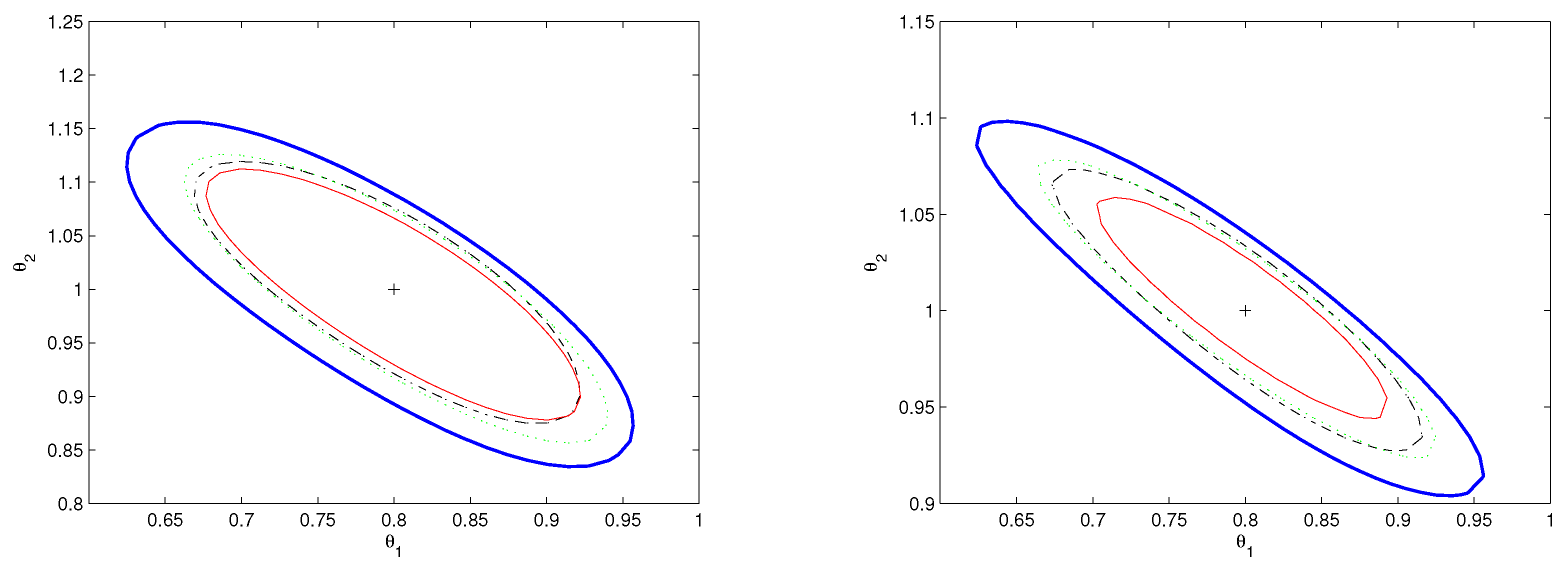
In order to construct confidence regions for the proposed estimators, it is essential to estimate their asymptotic variances ${\Sigma }_1$ and ${\Sigma }_2$ consistently from the sample $\{({\mathit{x}}_i,Y_i,{\delta }_i):i=1,\cdots ,n\}$. To achieve this, we employ the plug-in method in the simulation studies. For instance, the sample-based estimate ${\widehat{V}}_1$ of $V_1$ is

$${\widehat{V}}_1={\displaystyle \frac{1}{n}}\sum _{i=1}^n{\displaystyle \frac{{\delta }_i}{{\pi }^2({\mathit{x}}_i,Y_i;{\widehat{\mathit{\alpha }}}_p)}}{\varpi }^{-4}\left({\mathit{x}}_i\right)\nabla {\left({\widehat{\mathit{\theta }}}_1\right)}^{\otimes 2}{\widehat{\epsilon }}_i^2.$$

Other estimates for $\Gamma$, $V_2$, $B_1$, $B_2$, ${\Omega }_1$ and ${\Omega }_2$ can be obtained in a similar manner. We omit the details here for brevity.

While the plug-in method is effective in NMAR settings, it can be computationally intensive due to the complexity of the asymptotic variances involved. As an alternative, particularly when dealing with large datasets, the bootstrap procedure provides an effective approach for approximating these asymptotic variances. This method, which has been explored in studies such as those of Zhao et al. [30] and Jiang et al. [31] for NMAR data, can help alleviate computational challenges and provide more practical estimations in large-scale applications.

4. Simulation Study

Finite-sample performance of the proposed methods is evaluated through Monte Carlo experiments. For bandwidth selection, we implement the data-driven approaches of Zhou et al. [32] and Tang et al. [23], adopting the rule-of-thumb bandwidth: $h_n={\widehat{\sigma }}_X{n}^{-1/3}$, where ${\widehat{\sigma }}_X$ denotes the sample standard deviation of the observed covariate X. This practical bandwidth selector balances asymptotic optimality and computational simplicity.

4.1. Simulation 1

Let $f({\mathbf{x}}_i;\mathit{\theta })=exp\left(X_{i1}{\theta }_1+X_{i2}{\theta }_2\right)$, and $\varpi \left({\mathbf{x}}_i\right)=\sqrt{exp\left(X_{i1}{X}_{i2}\right)}$. The true parameter is set as ${\mathit{\theta }}_0={(0.8,1)}^{\top }$, and the error term ${\epsilon }_i\sim N(0,0.5^2)$. The covariates are generated under two scenarios: In Model A, $X_{i1}$ and $X_{i2}$ are independently sampled from $U(0,1)$; in Model B, $X_{i1}\sim U(0,1)$ while $X_{i1}=X_{i2}+{\epsilon }_i^{*}$ (${\epsilon }_i^{*}\sim U(-1,1)$), allowing us to examine the impact of covariate dependence. We implement a sample size of $n=150$, with response variables generated following the specification in model (1).

The missing indicator follows the nonignorable mechanism

$${\delta }_i\sim \mathrm{Bernoulli}\left(\pi ({\mathbf{x}}_i,Y_i;\mathit{\alpha })\right),\pi ({\mathbf{x}}_i,Y_i;\mathit{\alpha })={\displaystyle \frac{exp({\alpha }_0+{\alpha }_y{Y}_i)}{1+exp({\alpha }_0+{\alpha }_y{Y}_i)}},$$

where $\mathit{\alpha }={(0.05,0.05)}^{\top }$. The covariates $X_{i1}$ and $X_{i2}$ serve as instrumental variables. The parameter $\mathit{\alpha }$ is estimated using the penalized semiparametric likelihood method, incorporating the following auxiliary information matrix:

$$\begin{array}{c}\hfill \Delta ({\mathbf{x}}_i,Y_i;\mathit{\alpha })=\left(\begin{array}{c}{\delta }_i{\pi }^{-1}({\mathbf{x}}_i,Y_i;\mathit{\alpha })(X_{i1}-\overline{X_1})\\ {\delta }_i{\pi }^{-1}({\mathbf{x}}_i,Y_i;\mathit{\alpha })(X_{i2}-\overline{X_2})\end{array}\right),\end{array}$$

where $\overline{X_1}=n^{-1}{\sum }_{i=1}^n{X}_{i1}$ and $\overline{X_2}=n^{-1}{\sum }_{i=1}^n{X}_{i2}$. We adopt the product Gaussian kernel $K(u_1,u_2)=e^{-(u_1^2+u_2^2)/2}/2\pi$ and set the bandwidth as $h={\widehat{\sigma }}_{X_1}{n}^{-1/3}$ following Tang et al. [23].

Based on 500 independent replications, the proposed penalized method achieves an average IV selection rate of 92.8% for $X_1$ and $X_2$, demonstrating its effectiveness. For Model A and Model B, the 95% confidence regions for parameter $\mathit{\theta }$ and their coverage probabilities are calculated based on the EL methods $\mathrm{EL}\left({\widehat{\mathit{\theta }}}_1\right)$ and $\mathrm{EL}\left({\widehat{\mathit{\theta }}}_2\right)$, as well as the normal approximation approaches $\mathrm{NA}\left({\widehat{\mathit{\theta }}}_1\right)$ and $\mathrm{NA}\left({\widehat{\mathit{\theta }}}_2\right)$. The simulation results for the confidence regions are displayed in Figure 1.

The left panel of Figure 1 presents the simulated confidence regions for Model A based on the four aforementioned approaches, whereas the right panel displays the corresponding results for Model B. Several notable findings emerge from Figure 1. First, the confidence regions constructed using EL approaches are smaller than those based on NA methods, indicating the superior efficiency of EL-based inference. Second, the EL-based confidence region for ${\widehat{\mathit{\theta }}}_2$ is smaller than that for ${\widehat{\mathit{\theta }}}_1$, highlighting the enhanced efficiency of the AIPW estimator relative to the IPW estimator. Third, even in the presence of correlation between covariates in Model B, the EL and NA approaches yield confidence regions similar to those in Model A, implying the stability of these methods. The coverage probabilities for all four approaches are comparable in models A and B, closely aligning with the nominal 95% level. Overall, the EL-based approaches demonstrate superior efficiency relative to the NA-based methods, and the AIPW-based estimation is shown to be more efficient than the IPW-based estimation.

4.2. Simulation 2

We consider the regression model with nonlinear components

$$Y_i={\theta }_0+\sum _{k=1}^4{\theta }_k{X}_{ik}+exp\left({\theta }_5{X}_{i5}\right)+0.5{\epsilon }_i,i=1,\dots ,n,$$

where the true parameter vector is ${\mathit{\theta }}_0={(2.5,0.5,-1.5,0.5,-1,0.5)}^{\top }$. The covariates ${\mathbf{x}}_i={(X_{i1},\dots ,X_{i5})}^{\top }$ follow the multivariate normal distribution ${\mathcal{N}}_5(\mathbf{0},\Sigma )$ with covariance matrix $\Sigma ={(0.5^{|i-j|})}_{5\times 5}$. The error terms ${\epsilon }_i$ are independently distributed as $N(0,1)$.

The nonresponse mechanism follows the nonignorable logistic model

$$\pi ({\mathbf{x}}_i,Y_i;\mathit{\alpha })={\left\{1+exp\left(-{\alpha }_0-\sum _{k=1}^5{\alpha }_k{X}_{ik}-{\alpha }_y{Y}_i\right)\right\}}^{-1},$$

where $\mathit{\alpha }={(0.5,0,0,0.8,0,0,0.5)}^{\top }$. The IV $\mathbf{z}=(X_1,X_2,X_4,X_5)$ is identified through the proposed penalized estimation process. To address high-dimensional challenges, we employ MAR-based propensity score estimation

$$\tilde{s}(\mathbf{x},{\widehat{\gamma }}^{*})={\left\{1+exp(-{\widehat{\gamma }}_0^{*}-{\widehat{\gamma }}_1^{*\top }\mathbf{x})\right\}}^{-1},$$

where ${\widehat{\gamma }}^{*}$ denotes the maximum likelihood estimates. This enables the construction of a semiparametric estimator

$${\widehat{m}}_{\phi }^0(\tilde{s},\mathit{\alpha },\mathit{\theta })={\displaystyle \frac{{\sum }_{i=1}^n{\delta }_{i}O({\mathbf{x}}_i,Y_i;\mathit{\alpha }){\mathcal{F}}_h(\tilde{s}-{\tilde{s}}_i)\phi ({\mathbf{x}}_i,Y_i;\mathit{\theta })}{{\sum }_{i=1}^n{\delta }_{i}O({\mathbf{x}}_i,Y_i;\mathit{\alpha }){\mathcal{F}}_h(\tilde{s}-{\tilde{s}}_i)}},$$

where ${\mathcal{F}}_h(·)$ represents a univariate kernel density function. For each data generating mechanism, we generate 500 Monte Carlo random samples of sizes 150 and 250.

Table 1. Simulation results on the estimation performance of $\mathit{\alpha }$ in Simulation 2.

	$\mathit{n}=150$					$\mathit{n}=250$
Est.	Bias	SD	RMS	T	F	Bias	SD	RMS	T	F
${\widehat{\alpha }}_0$	0.0549	0.1021	0.1158	3.69	0	0.0447	0.0703	0.0833	3.79	0
${\widehat{\alpha }}_3$	0.0211	0.2313	0.2321	–	–	0.0038	0.1612	0.1612	–	–
${\widehat{\alpha }}_y$	0.0031	0.1397	0.1397	–	–	0.0118	0.0984	0.0990	–	–

summarizes the finite-sample performance of the proposed method, presenting three key metrics for nonzero components in $\mathit{\alpha }$: empirical bias (Bias), root mean square (RMS) error, and standard deviation (SD). The variable selection outcomes are quantified through two measures: “T” (mean count of correctly excluded irrelevant variables) and “F” (mean count of erroneously excluded significant variables).

Table 2. Simulation results on the estimation performance of $\mathit{\theta }$ in Simulation 2.

		IPW			AIPW
$\mathit{n}$	Est.	Bias	SD	RMS	Bias	SD	RMS
150	${\widehat{\theta }}_0$	0.0014	0.0442	0.0443	0.0007	0.0439	0.0439
	${\widehat{\theta }}_1$	0.0015	0.0519	0.0520	0.0012	0.0520	0.0522
	${\widehat{\theta }}_2$	0.0015	0.0569	0.0570	0.0008	0.0576	0.0576
	${\widehat{\theta }}_3$	0.0006	0.0596	0.0596	0.0001	0.0601	0.0601
	${\widehat{\theta }}_4$	0.0023	0.0573	0.0574	0.0020	0.0574	0.0574
	${\widehat{\theta }}_5$	0.0011	0.0305	0.0305	0.0009	0.0305	0.0305
250	${\widehat{\theta }}_0$	0.0006	0.0382	0.0382	0.0008	0.0379	0.0379
	${\widehat{\theta }}_1$	0.0012	0.0399	0.0399	0.0012	0.0401	0.0402
	${\widehat{\theta }}_2$	0.0015	0.0466	0.0466	0.0013	0.0466	0.0466
	${\widehat{\theta }}_3$	0.0010	0.0450	0.0450	0.0013	0.0449	0.0449
	${\widehat{\theta }}_4$	0.0016	0.0409	0.0409	0.0021	0.0409	0.0409
	${\widehat{\theta }}_5$	0.0005	0.0227	0.0227	0.0007	0.0225	0.0225

compares the estimation accuracy of regression coefficients between IPW and AIPW approaches, reporting their respective bias, RMS, and SD values.

The principal findings emerge as follows:

(1) Variable Selection Efficacy: The penalized semiparametric likelihood method demonstrates robust variable selection capability in the nonresponse mechanism model, effectively distinguishing between relevant and irrelevant covariates.

(2) Estimation Precision: For active components in $\mathit{\alpha }$, the observed minimal bias with closely matched SD and RMS values confirms the estimator’s statistical efficiency.

(3) MELE Performance Consistency: For both ${\widehat{\mathit{\theta }}}_1$ and ${\widehat{\mathit{\theta }}}_2$, the SD and RMS are nearly identical, suggesting that the proposed method for MELEs effectively estimates parameters through the penalized parametric likelihood approach.

(4) Sample Size Effects: Enhanced estimation efficiency emerges with larger samples for both the missingness data model and regression model.

5. Application to the ACTG 175 Data

We demonstrate the proposed methodology using data from the AIDS Clinical Trials Group Protocol 175 (ACTG 175) involving 2139 HIV-infected participants (Hammer et al. [33]). Following the established analytical approaches of Davidian et al. [34], Tsiatis et al. [35], and Han [8], we classify treatments into two groups: zidovudine (ZDV) monotherapy (532 subjects) versus combined therapies (1607 subjects). The analysis focuses on CD4 counts at $96\pm 5$ weeks post-baseline ($Y=\mathrm{CD}{4}_{96}$) as the primary endpoint, with the following covariates:

• Treatment assignment ($X_1$: 0 = ZDV monotherapy)
• Baseline CD4 count ($X_2$: $\mathrm{CD}{4}_0$)
• Demographic covariates: age ($X_3$), weight ($X_4$), race ($X_5$: 0 = White), gender ($X_6$: 0 = Female)
• Clinical covariates: antiretroviral history ($X_7$: 0 = naive), early treatment termination ($X_8$: 0 = completed)

The binary indicator variable r encodes the missingness status of the response Y, where $r_i=1$ indicates an observed outcome, and $r_i=0$ denotes a missing value. Previous studies of Davidian et al. [34], Tsiatis et al. [35], and Han [8] assumed that the missingness mechanism depends solely on covariates through a MAR framework. Our penalized semiparametric likelihood approach enhances robustness by incorporating shrinkage estimation within the nonresponse mechanism model. Specifically, shrinkage of the response variable coefficient toward zero provides formal evidence supporting the MAR assumption, while a nonzero estimate suggests NMAR.

To facilitate direct comparison with Han [8], we specialize the general model (1) to a linear regression framework

$$Y={\theta }_1+\sum _{l=2}^9{\theta }_l{X}_{l-1}+\epsilon ,\mathrm{E}\left(\epsilon \right|\mathbf{X})=0,$$

(6)

where $X_1$–$X_8$ represent the baseline covariates defined previously. The nonresponse mechanism is parameterized via logistic regression

$$\mathrm{P}(r=1|\mathbf{X},Y)={\displaystyle \frac{exp\left({\alpha }_0+{\sum }_{k=1}^8{\alpha }_k{X}_k+{\alpha }_{9}Y\right)}{1+exp\left({\alpha }_0+{\sum }_{k=1}^8{\alpha }_k{X}_k+{\alpha }_{9}Y\right)}},$$

with parameter vector $\mathit{\alpha }={({\alpha }_0,\dots ,{\alpha }_9)}^{\top }$. To address dimensionality challenges, we implement the regularization strategy detailed in Section 4.2, constructing consistent estimators for $m_{\phi }^0(\mathbf{x};\mathit{\theta },\mathit{\alpha })$ through MAR-based nonresponse mechanism weighting.

The penalized semiparametric likelihood estimates are presented in

Table 3. Estimation of response model parameters $\mathit{\alpha }$.

Est.	Estimate	p-Value	Est.	Estimate	p-Value
${\widehat{\alpha }}_0$	0.64	<0.001	${\widehat{\alpha }}_5$	0.0068	<0.001
${\widehat{\alpha }}_1$	−0.0007	<0.001	${\widehat{\alpha }}_6$	0.0002	0.002
${\widehat{\alpha }}_2$	0.0011	0.003	${\widehat{\alpha }}_7$	0.0010	<0.001
${\widehat{\alpha }}_3$	0	0.574	${\widehat{\alpha }}_8$	−0.6299	<0.001
${\widehat{\alpha }}_4$	0	0.191	${\widehat{\alpha }}_9$	−0.0010	<0.001

, with p-values calculated using 200 bootstrap replications (Efron and Tibshirani [36]). The weight (${\alpha }_3$) and age (${\alpha }_4$) show nonsignificant contributions to the nonresponse mechanism, as their coefficients are shrunk to zero with p-values exceeding 0.1. The significant coefficient for CD4 counts at $96\pm 5$ weeks (${\mathit{\alpha }}_9$) indicates an NMAR in this dataset.

Table 4. Results of the analysis on the ACTG 175 data.

	Complete-Case Analysis			Han’s Method
	Estimate	s.e.	p-Value	Estimate	s.e.	p-Value
Intercept	21.50	27.44	0.433	65.53	34.06	0.054
Trt	63.68	9.09	<0.001	52.72	10.34	<0.001
$\mathrm{CD}{4}_0$	0.76	0.04	<0.001	0.73	0.05	<0.001
Age	0.10	0.45	0.816	0.14	0.55	0.796
Weight	0.54	0.28	0.054	0.27	0.33	0.417
Race	−20.60	8.51	0.015	−18.30	9.66	0.058
Gender	−10.73	10.79	0.320	−16.54	11.34	0.145
History	−42.02	7.62	<0.001	−41.45	8.65	<0.001
Offtrt	−80.72	9.62	<0.001	−86.87	10.31	<0.001
	IPW			AIPW
	Estimate	s.e.	p-Value	Estimate	s.e.	p-Value
Intercept	33.15	30.66	0.2796	34.28	30.77	0.2651
Trt	62.14	9.52	<0.001	61.77	9.60	<0.001
$\mathrm{CD}{4}_0$	0.76	0.05	<0.001	0.76	0.05	<0.001
Age	0.18	0.53	0.7278	0.18	0.54	0.7326
Weight	0.42	0.32	0.1797	0.42	0.32	0.1884
Race	−22.07	10.10	0.0288	−22.01	10.13	0.0297
Gender	−9.38	12.07	0.4369	−9.33	12.10	0.4402
History	−41.34	8.67	<0.001	−41.24	8.70	<0.001
Offtrt	−74.74	11.62	<0.001	−74.44	11.64	<0.001

presents the analysis results for model (6), with standard errors estimated through 200 bootstrap replications. The comparative results from the complete-case analysis and Han’s multiply robust method, as described by Han [8], are also included. The nonsignificant predictors include age, weight, and gender. The analysis reveals five critical clinical insights:

(1) Treatment Superiority: Combination antiretroviral therapies (Trt = 1) demonstrate significantly higher CD4 counts at $96\pm 5$ weeks compared to ZDV monotherapy, establishing the enhanced therapeutic effectiveness of newer regimens.

(2) Baseline Predictive Power: Baseline CD4 counts (CD4₀) show significant positive association with follow-up counts, confirming their prognostic value in HIV management.

(3) Racial Disparity: White patients maintain clinically significant CD4 count advantage over nonwhite counterparts, suggesting differential disease progression trajectories.

(4) Treatment History Impact: Antiretroviral-experienced patients exhibit substantially reduced CD4 counts compared to naive patients, indicating potential cumulative treatment effects.

(5) Adherence Consequences: Early treatment discontinuation associates with marked CD4 count reduction, underscoring the critical importance of sustained therapeutic engagement.

6. Conclusions and Future Work

We developed a penalized semiparametric likelihood approach that resolves the identification challenges in nonignorable missing data analysis. The proposed estimator achieves the oracle properties under appropriate tuning parameter selection as established in our theoretical framework. The construction of profile EL ratio functions incorporated IPW and AIPW estimating equations. Our analysis demonstrated that when using consistently estimated nonresponse mechanism parameters, the ELLRFs follow an asymptotic weighted ${\chi }^2$ distribution. Furthermore, we systematically established the asymptotic normality of regression parameter estimators. Simulation studies and real-data applications confirmed the method’s practical effectiveness in both parameter estimation and variable selection. Comparative analyses revealed superior performance over existing approaches in handling nonignorable nonresponse data.

In practical applications, nonlinear regression models often involve high-dimensional covariates, which can lead to sparsity within the model. The direct application of the proposed estimation procedure in such contexts may lead to biased estimates. One potential approach to address this challenge is the application of the penalized EL method, as studied by Ren and Zhang [37], for model selection. It could effectively balance the model complexity and goodness of fit, thereby reducing the bias induced by high-dimensional covariates. This extension requires a systematic and separate investigation within the NMAR framework. A detailed exploration of this important issue will be undertaken in future research.

References

1. Jennrich, R.I. Asymptotic properties of non-linear least squares estimators. Ann. Math. Stat. 1969, 40, 633–643. [Google Scholar] [CrossRef]
2. Wu, C.F. Asymptotic theory of nonlinear least squares estimation. Ann. Stat. 1981, 9, 501–513. [Google Scholar] [CrossRef]
3. Fekedulegn, D.; Mac Siurtain, M.P.; Colbert, J.J. Parameter estimation of nonlinear growth models in forestry. Silva Fenn 1999, 33, 327–336. [Google Scholar] [CrossRef]
4. Ivanov, A.V. Asymptotic Theory of Nonlinear Regression; Kluwer Academic Publishers: Dordrecht, The Netherlands, 1997. [Google Scholar]
5. Little, R.J.; Rubin, D.B. Statistical Analysis with Missing Data; John Wiley & Sons: New York, NY, USA, 2019. [Google Scholar]
6. Horvitz, D.G.; Thompson, D.J. A generalization of sampling without replacement from a finite universe. J. Am. Stat. Assoc. 1952, 47, 663–685. [Google Scholar] [CrossRef]
7. Robins, J.M.; Rotnitzky, A.; Zhao, L. Estimation of regression coefficients when some regressors are not always observed. J. Am. Stat. Assoc. 1994, 89, 846–866. [Google Scholar] [CrossRef]
8. Han, P. Multiply robust estimation in regression analysis with missing data. J. Am. Stat. Assoc. 2014, 109, 1159–1173. [Google Scholar] [CrossRef]
9. Xue, L.; Xie, J. Efficient robust estimation for single-index mixed effects models with missing observations. Stat. Pap. 2024, 65, 827–864. [Google Scholar] [CrossRef]
10. Sharghi, S.; Stoll, K.; Ning, W. Statistical inferences for missing response problems based on modified empirical likelihood. Stat. Pap. 2024, 65, 4079–4120. [Google Scholar] [CrossRef]
11. Li, W.; Luo, S.; Xu, W. Calibrated regression estimation using empirical likelihood under data fusion. Comput. Stat. Data Anal. 2024, 190, 107871. [Google Scholar] [CrossRef]
12. Tang, N.; Zhao, P. Empirical likelihood-based inference in nonlinear regression models with missing responses at random. Statistics 2013, 47, 1141–1159. [Google Scholar] [CrossRef]
13. Owen, A.B. Empirical likelihood ratio confidence regions. Ann. Stat. 1990, 18, 90–120. [Google Scholar] [CrossRef]
14. Yang, Z.; Tang, N. Empirical likelihood for nonlinear regression models with nonignorable missing responses. Can. J. Stat. 2020, 48, 386–416. [Google Scholar] [CrossRef]
15. Wang, S.; Shao, J.; Kim, J.K. An instrumental variable approach for identification and estimation with nonignorable nonresponse. Stat. Sin. 2014, 24, 1097–1116. [Google Scholar] [CrossRef]
16. Wang, L.; Shao, J.; Fang, F. Propensity model selection with nonignorable nonresponse and instrument variable. Stat. Sin. 2021, 31, 647–672. [Google Scholar] [CrossRef]
17. Chen, J.; Shao, J.; Fang, F. Instrument search in pseudo-likelihood approach for nonignorable nonresponse. Ann. Inst. Stat. Math. 2021, 73, 519–533. [Google Scholar] [CrossRef]
18. Du, J.; Li, Y.; Cui, X. Identification and estimation of generalized additive partial linear models with nonignorable missing response. Commun. Math. Stat. 2024, 12, 113–156. [Google Scholar] [CrossRef]
19. Beppu, K.; Morikawa, K. Verifiable identification condition for nonignorable nonresponse data with categorical instrumental variables. Stat. Theory Relat. Fields. 2024, 8, 40–50. [Google Scholar] [CrossRef]
20. Fan, J.; Li, R. Variable selection via nonconcave penalized likelihood and its oracle properties. J. Am. Stat. Assoc. 2001, 96, 1348–1360. [Google Scholar] [CrossRef]
21. Qin, J.; Leung, D.; Shao, J. Estimation with survey data under nonignorable nonresponse or informative sampling. J. Am. Stat. Assoc. 2002, 97, 193–200. [Google Scholar] [CrossRef]
22. Qin, J.; Lawless, J.F. Empirical likelihood and general estimating equations. Ann. Stat. 1994, 22, 300–325. [Google Scholar] [CrossRef]
23. Tang, N.; Zhao, P.; Zhu, H. Empirical likelihood for estimating equations with nonignorably missing data. Stat. Sin. 2014, 24, 723–747. [Google Scholar] [CrossRef] [PubMed]
24. Ding, X.; Tang, N. Adjusted empirical likelihood estimation of distribution function and quantile with nonignorable missing data. J. Syst. Sci. Complex. 2018, 31, 820–840. [Google Scholar] [CrossRef]
25. Morikawa, K.; Kano, Y. Statistical inference with different missing-data mechanisms. arXiv 2014, arXiv:1407.4971. [Google Scholar]
26. Miao, W.; Tchetgen, E.J. On varieties of doubly robust estimators under missingness not at random with a shadow variable. Biometrika 2016, 103, 475–482. [Google Scholar] [CrossRef]
27. Liu, T.; Yuan, X. Doubly robust augmented-estimating-equations estimation with nonignorable nonresponse data. Stat. Pap. 2020, 61, 2241–2270. [Google Scholar] [CrossRef]
28. Zhao, P.; Tang, N.; Zhu, H. Generalized empirical likelihood inferences for nonsmooth moment functions with nonignorable missing values. Stat. Sin. 2020, 30, 217–249. [Google Scholar]
29. Hu, Z.; Follmann, D.A.; Qin, J. Semiparametric dimension reduction estimation for mean response with missing data. Biometrika 2010, 97, 305–319. [Google Scholar] [CrossRef]
30. Zhao, P.; Tang, N.; Qu, A.; Jiang, D. Semiparametric estimating equations inference with nonignorable missing data. Stat. Sin. 2017, 27, 89–113. [Google Scholar]
31. Jiang, D.; Zhao, P.; Tang, N. A propensity score adjustment method for regression models with nonignorable missing covariates. Comput. Stat. Data Anal. 2016, 94, 98–119. [Google Scholar] [CrossRef]
32. Zhou, Y.; Wan, A.T.K.; Wang, X. Estimating equations inference with missing data. J. Am. Stat. Assoc. 2008, 103, 1187–1199. [Google Scholar] [CrossRef]
33. Hammer, S.M.; Katzenstein, D.A.; Hughes, M.D.; Gundacker, H.; Schooley, R.T.; Haubrich, R.H.; Henry, W.K.; Lederman, M.M.; Phair, J.P.; Niu, M.; et al. A trial comparing nucleoside monotherapy with combination therapy in HIV-infected adults with CD4 cell counts from 200 to 500 per cubic millimeter. N. Engl. J. Med. 1996, 335, 1081–1090. [Google Scholar] [CrossRef] [PubMed]
34. Davidian, M.; Tsiatis, A.A.; Leon, S. Semiparametric estimation of treatment effect in a pretest–posttest study with missing data. Statist. Sci. 2005, 20, 261–301. [Google Scholar] [CrossRef] [PubMed]
35. Tsiatis, A.A.; Davidian, M.; Zhang, M.; Lu, X. Covariate adjustment for two-sample treatment comparisons in randomized clinical trials: A principled yet flexible approach. Stat. Med. 2008, 27, 4658–4677. [Google Scholar] [CrossRef]
36. Efron, B.; Tibshirani, R.J. An Introduction to the Bootstrap; Chapman & Hall: New York, NY, USA, 1993. [Google Scholar]
37. Ren, Y.; Zhang, X. Variable selection using penalized empirical likelihood. Sci. China Math. 2011, 54, 1829–1845. [Google Scholar] [CrossRef]
Figure 1. Simulation 1 results comparing EL and NA methods. Line specifications: EL ( θ ^ 2 ) (red solid), EL ( θ ^ 1 ) (green dotted), NA ( θ ^ 2 ) (black dash-dot), NA ( θ ^ 1 ) (blue thick solid).
Mathematics 13 01388 g001