Article

Ninth-Order Two-Step Methods with Varying Step Lengths

by
Rubayyi T. Alqahtani
1,
Theodore E. Simos
2,* and
Charalampos Tsitouras
3
1
Department of Mathematics and Statistics, College of Science, Imam Mohammad Ibn Saud Islamic University (IMSIU), Riyadh 11623, Saudi Arabia
2
Center for Applied Mathematics and Bioinformatics, Gulf University for Science and Technology, West Mishref 32093, Kuwait
3
General Department, National & Kapodistrian University of Athens, GR34-400 Euripus Campus, Greece
*
Author to whom correspondence should be addressed.
Mathematics 2025, 13(8), 1257; https://doi.org/10.3390/math13081257
Submission received: 5 March 2025 / Revised: 30 March 2025 / Accepted: 6 April 2025 / Published: 11 April 2025
(This article belongs to the Special Issue Numerical Methods Applied to Mathematical Problems)

Abstract

:
This study investigates a widely recognized ninth-order numerical technique within the explicit two-step family of methods (a.k.a. hybrid Numerov-type methods). To boost its performance, we incorporate an economical step-size control algorithm that, after each iteration, either preserves the current step length, reduces it by half, or doubles it. Any additional off-grid points needed by this strategy are computed using a local interpolation routine. Indicative numerical experiments confirm the substantial efficiency gains realized by this method. It is particularly adept at resolving differential equations with oscillatory dynamics, delivering high precision with fewer function evaluations. Furthermore, a detailed Mathematica implementation is supplied, enhancing usability and fostering further research in the field. By simultaneously improving computational efficiency and accuracy, this work offers a significant contribution to the numerical analysis community.

1. Introduction

Our research delves into a specific type of second-order initial value problem (IVP), characterized by the following equation:
ψ = f ( x , ψ ) , ψ ( x 0 ) = ψ 0 , ψ ( x 0 ) = ψ 0 ,
where
f : R × R ν R ν and ψ 0 , ψ 0 R ν .
Notably, ψ does not appear explicitly in (1).
The Numerov method is a well-established numerical technique for advancing the solution from x κ to x κ + 1 = x κ + h . Its formula is given by the following:
ψ κ + 1 = 2 ψ κ ψ κ 1 + h 2 12 f κ + 1 + 10 f κ + f κ 1 ,
where
ψ κ ψ ( x κ ) and f κ ψ ( x κ ) = f ( x κ , ψ κ ) ,
with f κ , ψ κ R ν .
Pioneers such as Hairer [1], Cash [2], and Chawla [3] introduced hybrid implicit Numerov-type methods approximately 40–45 years ago. These methods utilized off-grid points and addressed the challenge of P-stability, which is crucial for stiff oscillatory problems. Later, Chawla [4] proposed a modified explicit Numerov scheme:
v 1 = ψ κ 1 , v 2 = ψ κ , v 3 = 2 ψ κ ψ κ 1 + h 2 f ( x κ , v 2 ) , ψ κ + 1 2 ψ κ + ψ κ 1 = 1 12 h 2 f ( x κ + 1 , v 3 ) + 10 f ( x κ , v 2 ) + f ( x κ 1 , v 1 ) ,
where h is the constant step size:
h = x κ x κ 1 = x κ + 1 x κ = = x 1 x 0 .
The vectors ψ κ + 1 , ψ κ , ψ κ 1 approximate ψ ( x κ + h ) , ψ ( x κ ) , ψ ( x κ h ) , respectively, while the stages v 1 , v 2 , v 3 R ν represent the function evaluations used by the method. We leverage the information at the grid:
v 1 = ψ κ 1 , v 2 = ψ κ .
Given that f ( x κ 1 , v 1 ) is calculated in the previous step, only f ( x κ + 1 , v 3 ) and f ( x κ , v 2 ) need to be evaluated at each step, resulting in just two function evaluations per step.
Following this, Tsitouras developed a technique drawing inspiration from Runge–Kutta–Nyström (RKN) methods [5], which significantly reduced computational overhead. As a result, only four steps are required to construct a sixth-order method, whereas earlier approaches necessitated six function evaluations (see [6]). Building upon this progress, our research group has extensively explored this topic. Tsitouras developed eighth-order methods that require nine steps per iteration in [7], and concurrently, a team of Spanish researchers conducted notable studies on similar problems [8,9,10].
A distinction must be made between the term “second-order initial value problem”, which signifies the presence of ψ , and the algebraic order of a numerical scheme, which defines its degree of precision.
Despite these advancements, current numerical methods often struggle with efficiency when applied to differential equations with oscillatory behavior. Our work addresses this limitation by optimizing the step-length adjustment in a ninth-order Numerov-type method, thereby considerably enhancing computational performance.
Here, we present a ninth-order Numerov-type approach that uniquely integrates a variable step-length algorithm, substantially improving computational efficiency for solving second-order IVPs with oscillatory behavior. This study aims to introduce a novel method specifically designed to better handle problems with periodic solutions. Traditionally, various characteristics of a basic test equation are utilized for this purpose; our innovation involves fine-tuning the free parameters across a broad range of relevant problems. Differential evolution is employed for this optimization, and we anticipate that this strategy will yield a method exceptionally well-suited for oscillatory challenges.
The main contributions of this work are as follows:
  • The construction of a ninth-order two-step method with variable step lengths, tailored for second-order oscillatory problems;
  • The development of an embedded error estimation mechanism enabling efficient step-size control through symbolic interpolation;
  • A detailed Mathematica implementation that facilitates symbolic order verification and adaptive logic; and (iv) numerical evidence demonstrating the method’s practical advantages in terms of accuracy and computational efficiency on classical orbital problems such as the Kepler and Arenstorf systems.

2. Derivation of Hybrid Numerov Methods

To address the given problem via advanced algebraic methodologies, we first express the independent parameter t as a component of ψ . Consequently, without any loss of generality, we concentrate on the autonomous formulation:
ψ = f ( ψ ) .
A blended Numerov algorithm utilizing s stages (as delineated in [7]) is formulated as follows:
ψ κ + 1 = 2 ψ κ ψ κ 1 + h 2 · b I s · f v v = 1 + c ψ κ c ψ κ 1 + h 2 · A I s · f v
where I s R s   ×   s denotes the identity matrix, and A R s   ×   s , b T R s , and c R s signify the coefficient matrices of the approach, with the following:
1 = [ 1 1 1 ] T R s .
To delineate these coefficients, we employ the Butcher tableau [11,12]:
c A b .
Since the function assessments are conducted in a sequential manner, these techniques are explicit, implying that A is a strictly lower triangular matrix. For the scenario where s = 9 , the matrices assume the following configuration:
f κ 1 = f x κ 1 , ψ κ 1 = ψ κ 1 , f κ = f x κ , ψ κ = ψ κ , ψ α = c 3 ψ κ 1 + 1 c 3 ψ κ + h 2 a 31 f κ 1 + a d 2 f κ , f α = f x κ + c 3 h , ψ α , ψ β = c 4 ψ κ 1 + 1 c 4 ψ κ + h 2 a 41 f κ 1 + a 42 f κ + a 43 f α , f β = f x κ + c 4 h , ψ β , ψ γ = c 5 ψ κ 1 + 1 c 5 ψ κ + h 2 a 51 f κ 1 + a 52 f κ + a 53 f α + a 54 f β , f γ = f x κ + c 5 h , ψ γ , ψ δ = c 6 ψ κ 1 + 1 c 6 ψ κ + h 2 a 61 f κ 1 + a 62 f κ + a 63 f α + a 64 f β + a 65 f γ , f δ = f x κ + c 6 h , ψ δ , ψ ϵ = c 7 ψ κ 1 + 1 c 7 ψ κ + h 2 a 71 f κ 1 + a 72 f κ + a 73 f α + a 74 f β + a 75 f γ + a 76 f δ , f ϵ = f x κ + c 7 h , ψ ϵ , ψ ζ = c 8 ψ κ 1 + 1 c 8 ψ κ + h 2 a 81 f κ 1 + a 82 f κ + a 83 f α + a 84 f β + a 85 f γ + a 86 f δ + a 87 f ϵ , f ζ = f x κ + c 8 h , ψ ζ , ψ η = c 9 ψ κ 1 + 1 c 9 ψ κ + h 2 a 91 f κ 1 + a 92 f κ + a 93 f α + a 94 f β + a 95 f γ + a 96 f δ + a 97 f ϵ + a 98 f ζ , f η = f x κ + c 9 h , ψ η , ψ κ + 1 = 2 ψ κ ψ κ 1 + h 2 b 1 f κ 1 + b 2 f κ + b 3 f α + b 4 f β + b 4 f γ + b 6 f δ + b 6 f ϵ + b 1 f ζ + b 1 f η .
Since we assumed the following above:
b 3 = 0 , b 5 = b 4 , b 7 = b 6 , b 8 = b 1 , c 5 = c 4 , c 7 = c 6 , c 8 = 0 , c 9 = 1 ,
the associated matrices take the following form:
A = 0 0 0 0 0 0 0 0 0 0 0 0 0 0 0 0 0 0 a 31 a 32 0 0 0 0 0 0 0 a 41 a 42 a 43 0 0 0 0 0 0 a 51 a 52 a 53 a 54 0 0 0 0 0 a 61 a 62 a 63 a 64 a 65 0 0 0 0 a 71 a 72 a 73 a 74 a 75 a 76 0 0 0 a 81 a 82 a 83 a 84 a 85 a 86 a 87 0 0 a 91 a 92 a 93 a 94 a 95 a 96 a 97 a 98 0 ,
b = b 1 b 2 0 b 4 b 4 b 6 b 6 b 1 b 1
and
c = 1 0 c 3 c 4 c 4 c 6 c 6 0 1 T .
Since f κ 1 is derived from the preceding iteration, only seven function evaluations are required per step. To attain an algebraic order of eight, it is crucial to eliminate the corresponding truncation error components (refer to [13]).
The proposed technique comprises a total of 34 parameters. As previously highlighted, there exist 27 coefficients associated with the matrix A, explicitly:
a 31 , a 32 , a 41 , a 42 , a 43 , , a 87 .
Furthermore, 4 coefficients correspond to the vector b, while 3 components belong to the vector c. The total number of order conditions at different accuracy levels aligns with those of Runge–Kutta–Nyström techniques, as illustrated in Table 1. To obtain ninth-order precision, a total of
1 + 1 + 2 + 3 + 6 + 10 + 20 + 36 + 72 = 151
equations must be fulfilled. Conditions extending to the ninth order can be found in several tables within [13].
Since the number of available parameters is insufficient to match the number of governing equations—a difficulty similar to that encountered in the formulation of Runge–Kutta (RK) schemes—specific simplifying assumptions must be imposed. These reductions decrease the number of constraints, thereby minimizing the number of coefficients. Frequently employed simplifications include the following:
( A · 1 ) ( 3 8 ) = 1 2 c 2 + c ( 3 9 ) , ( A · c ) ( 3 8 ) = 1 6 c 3 c ( 3 9 ) , ( A · c 2 ) ( 4 8 ) = 1 12 c 4 + c ( 4 9 ) ,
where
c i = ( 1 ) i 0 c 3 i c 4 i ( c 4 ) i ( c 5 ) i c 5 i 1 T ,
and
c 0 = 1 1 1 1 1 1 1 1 T = 1 .
For indices satisfying μ 1 < μ 2 , the notation
( v ) ( μ 1 μ 2 ) = [ v μ 1 v μ 1 + 1 v μ 2 ] T
is employed.
The additional order constraints are compiled in Table 2. Within this table, the notation “*” represents element-wise multiplication:
[ v 1 v 2 v n ] T [ u 1 u 2 u n ] T = [ v 1 u 1 v 2 u 2 v n u n ] T .
This operation has lower precedence, meaning that parentheses, exponentiation, and dot products are always evaluated before applying “*”.
Thus, we arrive at a nonlinear system consisting of 23 equations involving 23 unknown coefficients. For an in-depth discussion on deriving truncation error coefficients, the extensive review in [13] provides valuable insights. Coleman [14] highlighted the significance of the B2 series framework in analyzing the local truncation error, establishing links with T2 rooted tree structures.
To tackle this challenge, we adopt the differential evolution algorithm [15,16]. Differential evolution operates as an iterative optimization strategy where, at each iteration—termed generation λ —a “population” of candidate solutions is maintained, denoted as a 3 ( λ ) , a 4 ( λ ) , a 6 ( λ ) , w 1 ( λ ) , w 2 ( λ ) , , d 98 ( λ ) i , for i = 1 , 2 , , N , with N representing the population size. Initially, a starting population a 3 ( 0 ) , a 4 ( 0 ) , a 6 ( 0 ) , w 1 ( 0 ) , w 2 ( 0 ) , , d 98 ( 0 ) i , for i = 1 , 2 , , N , is randomly generated. The fitness function used for evaluation is defined as follows:
s = T 1 ( 1 ) 2 + T 2 ( 3 ) 2 + T 6 ( 5 ) 2 + + T 7 ( 9 ) 2
which quantifies the residuals for the 23 governing equations listed in Table 2. Each candidate in the initial population is assessed based on this function, with the objective of minimizing its value.
Every iteration g involves a structured three-step process to refine each candidate solution. These phases include the following:
  • Mutation (Differentiation): Generating a new potential candidate based on variations within the existing population.
  • Crossover: Recombining individuals to introduce diversity.
  • Selection: Retaining the fittest individuals for the subsequent generation.
For implementation, we employed the DeMat software [17] within the MATLAB environment [18], which incorporates this evolutionary strategy. Since a single execution does not guarantee optimal results, we conducted several hundred runs of the optimization process to ensure convergence to a viable solution. The obtained result was then further refined to greater accuracy using multi-precision arithmetic, employing the NMinimize function in Mathematica [19].
The specific parameters that yield an optimal ninth-order scheme Num9s8 are documented in [20] and can be found implemented in http://users.uoa.gr/~tsitourasc/NumerovSol9.m (accessed on 5 March 2025).

3. Variable Step Implementation

To establish a variable step-size algorithm, it is necessary to devise an error estimator. A similar strategy was used for 8th-order methods [21]. Here, we introduce an auxiliary vector
b ˜ = [ b ˜ 1 b ˜ 2 b ˜ 3 b ˜ 4 b ˜ 5 b ˜ 6 b ˜ 7 b ˜ 8 b ˜ 9 ] ,
with the aim of determining its coefficients so that the solution is approximated locally with sixth-order accuracy, i.e., with an error of O ( h 8 ) . Consequently, the following order conditions must be satisfied:
b ˜ e = 1 , b ˜ c = 0 , b ˜ c 3 = 0 , b ˜ c 2 = 1 6 , b ˜ c 4 = 1 15 , b ˜ c 5 = 0 , 1 120 b ˜ c + 1 120 b ˜ A c + b ˜ A 2 c = 0 .
We have obtained a solution for these coefficients, which is provided in the method’s implementation in Appendix A. Notably, no additional order conditions are required since the row-simplifying assumption (4) allows the other conditions to be eliminated.
The resulting, cost-free sixth-order approximation is given by the following:
ψ ˜ κ + 1 2 ψ κ + ψ κ 1 = h κ 2 · b ˜ 1 f κ 1 + b ˜ 2 f κ + b ˜ 3 f α + b ˜ 4 f β + b ˜ 5 f γ + b ˜ 6 f δ + b ˜ 7 f ϵ + b ˜ 8 f ζ + b ˜ 9 f η .
Thus, we obtain two approximations—one of order nine and one of order six—without any extra cost. By subtracting these approximations, we derive an O ( h 8 ) estimate of the local error:
E = ψ κ + 1 ψ ˜ κ + 1 = h κ 2 · ( b 1 b ˜ 1 ) f κ 1 + ( b 2 b ˜ 2 ) f κ + ( b 3 b ˜ 3 ) f α + ( b 4 b ˜ 4 ) f β + ( b 5 b ˜ 5 ) f γ + ( b 6 b ˜ 6 ) f δ + ( b 7 b ˜ 7 ) f ϵ + ( b 8 b ˜ 8 ) f ζ + ( b 9 b ˜ 9 ) f η .
We set a tolerance τ and keep the step unchanged if 32 τ > E > τ / 32 . If E < τ / 32 , we double the step for the next interval. In this way, using the available data ψ κ 1 , ψ κ 1 and ψ κ + 1 , ψ κ + 1 , we can compute the subsequent approximation as follows:
ψ κ + 2 = ψ x κ + 1 + 2 h κ + O ( h 8 ) = ψ x κ + 1 + h κ + 1 + O ( h 8 ) ( locally ) .
Proper adjustments in the indices are applied; see Figure 1 for a graphical illustration.
If instead E > 32 τ , we reject the trial step h ˜ κ = h κ 1 and instead compute the solution at x κ + 1 2 h ˜ κ = x κ + h κ , where h κ is the halved step used for advancing the solution. We then use ψ κ , ψ κ and suitable approximations for ψ κ 1 2 , ψ κ 1 2 to apply methods of the form (3), after adjusting indices appropriately (see Figure 2 for details).
A local O ( h 11 ) approximation for ψ κ 1 2 and h 2 ψ κ 1 2 is necessary to prevent order reduction due to error propagation. Such approximations can be obtained by applying the interpolation theory as introduced in [22]. Specifically, we add four additional stages f 1 , f 2 , f 3 and f 4 :
ψ 1 = c 10 ψ κ 1 + 1 c 10 ψ κ + h κ 2 ( a 10 , 1 f κ 1 + a 10 , 2 f κ + a 10 , 3 f α + a 10 , 4 f β + a 10 , 5 f γ + a 10 , 6 f δ + a 10 , 7 f ϵ + a 10 , 8 f ζ + a 10 , 9 f η ) , f 1 = f x κ + c 10 h κ , ψ 1 ,
ψ 2 = c 11 ψ κ 1 + 1 c 11 ψ κ + h κ 2 ( a 11 , 1 f κ 1 + a 11 , 2 f κ + a 11 , 3 f α + a 11 , 4 f β + a 11 , 5 f γ + a 11 , 6 f δ + a 11 , 7 f ϵ + a 11 , 8 f ζ + a 11 , 9 f η + a 11 , 10 f 1 ) , f 2 = f x κ + c 11 h κ , ψ 2 ,
ψ 3 = c 12 ψ κ 1 + 1 c 12 ψ κ + h κ 2 ( a 12 , 1 f κ 1 + a 12 , 2 f κ + a 12 , 3 f α + a 12 , 4 f β + a 12 , 5 f γ + a 12 , 6 f δ + a 12 , 7 f ϵ + a 12 , 8 f ζ + a 12 , 9 f η + a 12 , 10 f 1 + a 12 , 11 f 2 ) , f 3 = f x κ + c 12 h κ , ψ 3 ,
and
ψ 4 = c 13 ψ κ 1 + 1 c 13 ψ κ + h κ 2 ( a 13 , 1 f κ 1 + a 13 , 2 f κ + a 13 , 3 f α + a 13 , 4 f β + a 13 , 5 f γ + a 13 , 6 f δ + a 13 , 7 f ϵ + a 13 , 8 f ζ + a 13 , 9 f η + a 13 , 10 f 1 + a 13 , 11 f 2 + a 13 , 12 f 3 ) , f 4 = f x κ + c 12 h κ , ψ 4 .
This yields the following:
ψ κ 1 2 = 1 2 ψ κ + 1 2 ψ κ 1 + h κ 2 b ^ 1 f κ 1 + b ^ 2 f κ + b ^ 3 f α + b ^ 4 f β + b ^ 5 f γ + b ^ 6 f δ + b ^ 7 f ϵ + b ^ 8 f ζ + b ^ 9 f η + b ^ 10 f 1 + b ^ 11 f 2 + b ^ 12 f 3 + b ^ 13 f 4 = ψ x κ 1 2 h κ + O ( h 11 ) ,
where the approximations (i.e., big O notation) are considered locally.
Accordingly,
ψ x κ 1 2 h κ f x κ 1 2 h κ , ψ κ 1 2 = ψ κ 1 2 .
It is evident that rejecting a step incurs a cost of 12 function evaluations compared to the 8 evaluations used in a conventional step—namely, the usual seven stages f α , f β , f γ , f δ , f ϵ , f ζ , f η plus the extra stages f 1 , f 2 f 3 f 4 and the evaluation of f x κ 1 2 h κ , ψ κ 1 2 . Stage f k remains unchanged and is reused.
The set of new coefficients, i.e., b ^ , and the enhanced matrix, A ^ , containing original matrix A and c ^ = [ 1 , 0 , c 3 , c 4 , c 4 , c 6 , c 6 , 0 , 1 , c 10 , c 11 , c 12 , c 13 ] T , have to fulfill a modified set of 151 order conditions. This set has the form shown in Table 3 (see [22]). Here, we set ρ = 1 2 to properly approximate ψ κ 1 2 .
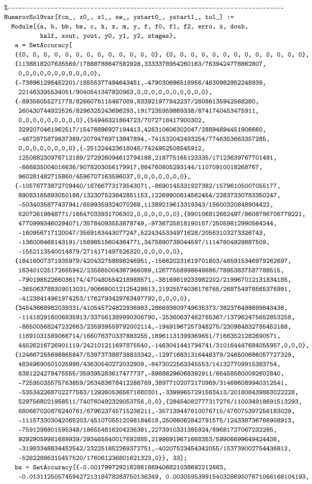
All coefficients are provided in the Mathematica listing in the appendix. It can also be retrieved from http://users.uoa.gr/~tsitourasc/NumerovSol9var.m (accessed on 5 March 2025), where we have implemented the method in Mathematica format. In that file, we also include, in a separate section, the verification of the given coefficients over the 151 equations of the condition for the interpolatory approximation of ψ κ 1 2 described above.

4. Numerical Tests

The innovative variable step method is designated as NumerovSol9var, reflecting its connection to Numerov, its 9th-order accuracy, and its variable step capability. It is compared with a method labeled as Num8s9 in [20] which is the underlying method here when the step is kept constant. This comparison is justified because Num8s9 has demonstrated superior performance over other methods of similar or lower orders, as evidenced in [20].
Initially, we implement the new method with various tolerance settings, documenting the number of stages used alongside the precision achieved for approximations of ψ at the endpoint. Subsequently, at a comparable computational cost (i.e., the total number of stages utilized in the variable step implementation), we execute the constant step method Num9s8 and also record the precision at the endpoint. The results are presented in efficiency curves. All tests were conducted using Mathematica.
The problems on which the methods were evaluated are as follows.

4.1. The Two-Body Problem

At the outset, we select the well-known two-body problem (a.k.a., Kepler problem), characterized by eccentricity e:
ψ 1 = y 1 ( ψ 1 2 + ψ 2 2 ) 3 / 2 , ψ 2 = ψ 2 ( ψ 1 2 + ψ 2 2 ) 3 / 2 , ψ 1 ( 0 ) = 1 e , ψ 1 = 0 , ψ 2 ( 0 ) = 0 , ψ 2 = 1 + e 1 e .
The Kepler problem, a fundamental issue in celestial mechanics, entails determining the trajectory of a planet or another celestial object influenced by a central gravitational force. Within the framework of this paper, the Kepler problem acts as a crucial test case for assessing the efficacy of the variable step-size implementation of the ninth-order hybrid Numerov-type method. Its significance in this research stems from its oscillatory characteristics and well-established periodic solutions, which offer a stringent evaluation of the new numerical technique’s effectiveness. By applying this method to such a classical problem, we can showcase its robustness and potential for wider applications in both theoretical and practical contexts involving differential equations with oscillatory dynamics.
Refer to [23] for the theoretical solution. It is important to note that in this problem’s definition, the indices correspond to the coordinates of ψ . We solved the aforementioned equation over the interval 0 , 6 π .
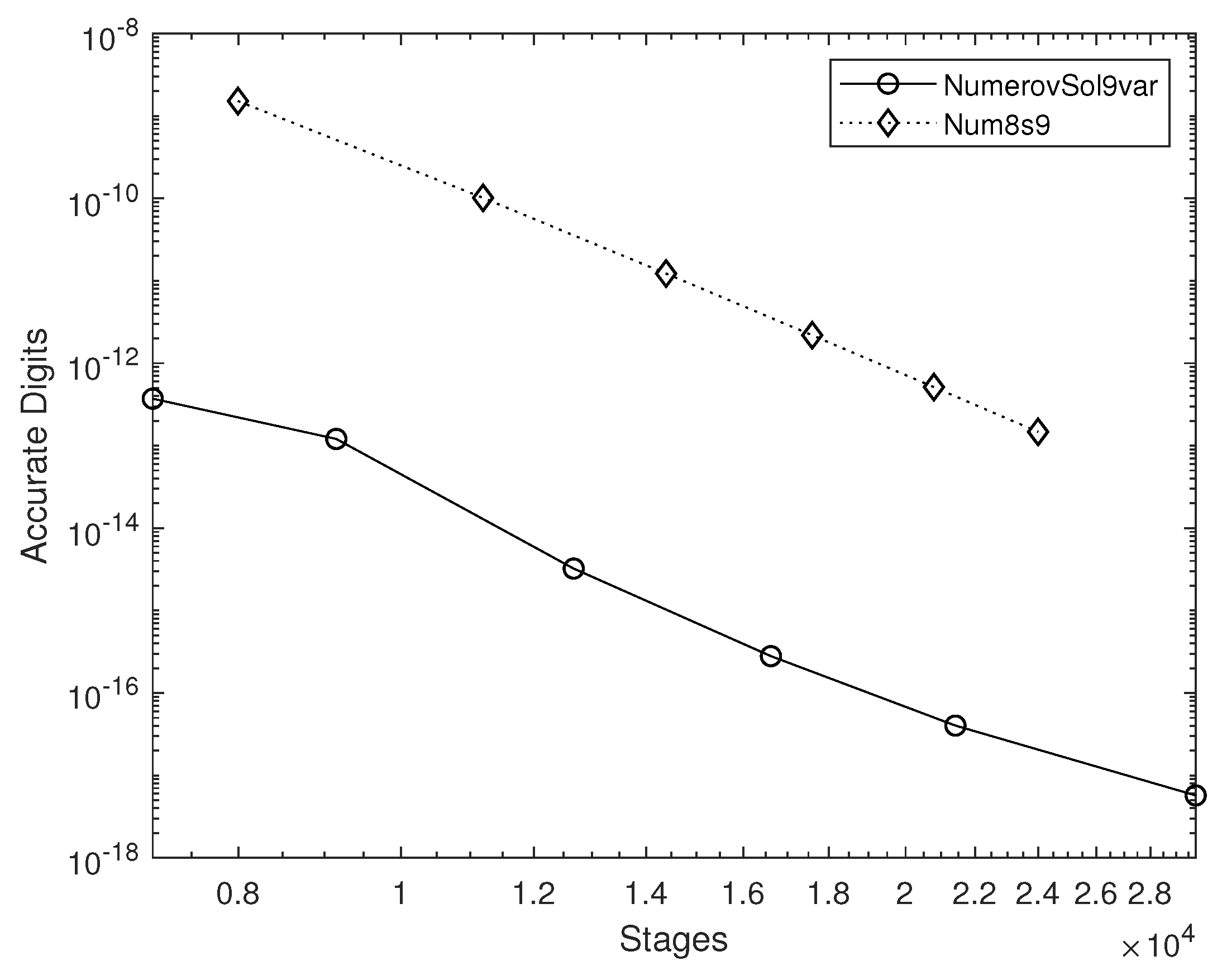
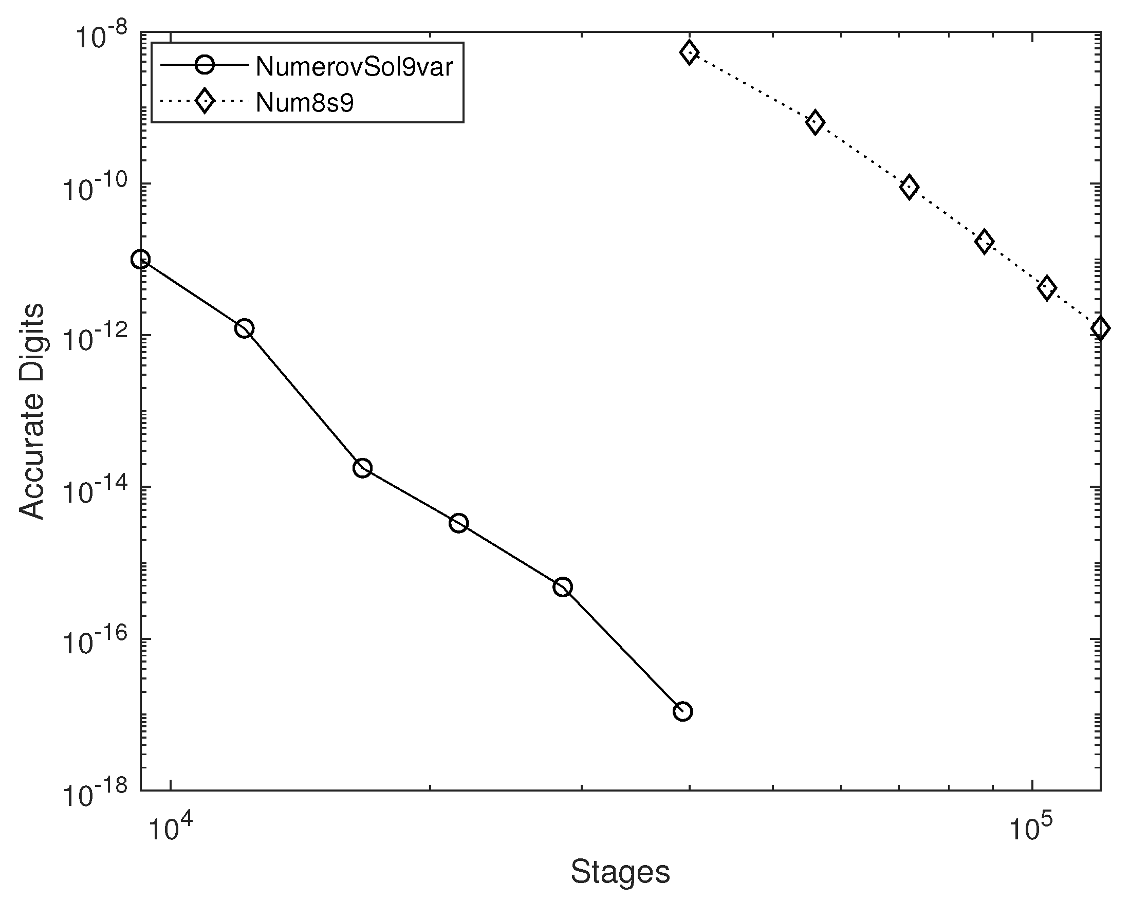
We examined three scenarios for eccentricities e = 0.5 (problem D3 of DETEST as outlined in [23]), e = 0.7 (problem D4 of DETEST), and e = 0.9 (problem D5 of DETEST), with results documented in Figure 3, Figure 4, and Figure 5, respectively. These findings demonstrate that utilizing the variable step algorithm provides a distinct advantage.
In the context of an elliptical solution (i.e., when e > > 0 ), the significant gain in precision is evident for NumerovSol9var across all scenarios. However, when applying an eccentricity of e = 0.9 , the difference becomes pronounced. Although the proposed ninth-order Numerov-type method with variable step lengths offers considerable efficiency enhancements, its benefits may be less pronounced for problems that do not necessitate frequent step adjustments, such as the Kepler problem with zero eccentricity. Conversely, when rapidly changing dynamics are present (e.g., Kepler with high eccentricity), the ability to adjust the step size is of paramount importance.

4.2. The Arenstorf Problem

The Arenstorf orbit is a stable orbit between Earth and Moon [24]. In form (1), it reads [25], (p. 296).
ψ 1 = 1 μ μ cos x ψ 1 ψ 1 + μ cos x 2 + ψ 2 + μ sin x 2 + μ 1 μ cos x ψ 1 ψ 1 1 μ cos x 2 + ψ 2 1 μ sin x 2 ,
ψ 2 = 1 μ μ sin x ψ 2 ψ 1 + μ cos x 2 + ψ 2 + μ sin x 2 + μ 1 μ sin x ψ 2 ψ 1 1 μ cos x 2 + ψ 2 1 μ sin x 2 ,
with initial values:
ψ 1 ( 0 ) = 0.994 , ψ 1 ( 0 ) = 0 , ψ 2 ( 0 ) = 0 , ψ 2 ( 0 ) = 1.00758510637908252 ,
μ = 0.012277471 and end point x end = 17.0652165601579625589 .
The solution at end–point is as follows:
ψ 1 ( x end ) = 0.994 cos ( x end ) , ψ 2 ( x end ) = 0.994 sin ( x end ) ,
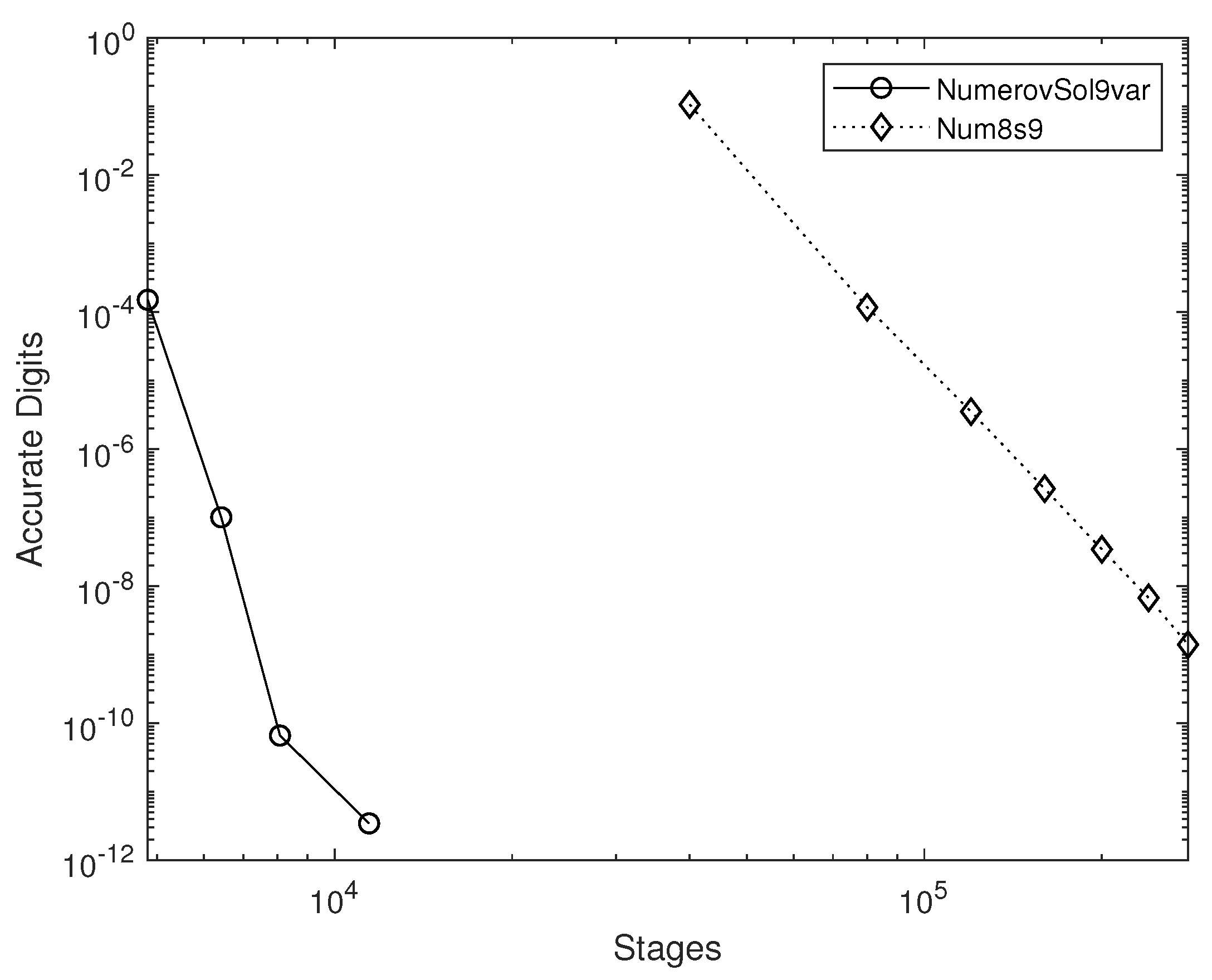
and the corresponding efficiency curves are shown in Figure 6.
Here, the results are really astonishing in favor of NumerovSol9var since the behavior of the solution requires many rapid and significant changes in the step size.

5. Conclusions

In this work, we introduced a novel ninth-order explicit two-step method equipped with a variable step-size mechanism specifically tailored for second-order initial value problems with oscillatory characteristics. The main contribution lies in the combination of high-order accuracy with a computationally efficient step-size control strategy, which employs error estimation through embedded methods and local interpolation to manage step doubling and halving.
We demonstrated the method’s performance across several challenging test problems, including the Kepler and Arenstorf orbits, where the proposed approach showed significant improvements in both accuracy and efficiency compared to fixed-step counterparts. The robustness of the method in handling stiff and rapidly varying dynamics underscores its potential for a wide range of scientific and engineering applications.
Moreover, the implementation in Mathematica, including symbolic verification of order conditions and adaptive control logic, enhances reproducibility and encourages further exploration by the research community.
Future work could investigate more flexible step-size control policies beyond binary step changes (doubling or halving), potentially guided by continuous error estimators. Additionally, extending the method to systems with variable coefficients, discontinuities, or multiphysics coupling would broaden its scope. The optimization of method parameters for specific subclasses of differential equations remains a promising direction for ongoing research.
Author Contributions

Conceptualization, R.T.A., T.E.S. and C.T.; Methodology, T.E.S. and C.T.; Software, R.T.A., T.E.S. and C.T.; Validation, R.T.A., T.E.S. and C.T.; Formal analysis, R.T.A., T.E.S. and C.T.; Investigation, R.T.A., T.E.S. and C.T.; Resources, T.E.S. and C.T.; Data curation, R.T.A., T.E.S. and C.T.; Writing—original draft, C.T.; Writing—review & editing, T.E.S.; Visualization, R.T.A., T.E.S. and C.T.; Supervision, T.E.S.; Project administration, T.E.S.; Funding acquisition, R.T.A. All authors have read and agreed to the published version of the manuscript.

Funding

This work was supported and funded by the Deanship of Scientific Research at Imam Mohammad Ibn Saud Islamic University (IMSIU) (grant number IMSIU-DDRSP-RP25).

Data Availability Statement

The MATLAB implementation containing the coefficients of the method presented can be retrieved from http://users.uoa.gr/~tsitourasc/NumerovSol9var.m (accessed on 5 March 2025).

Conflicts of Interest

The authors declare no conflicts of interest.

Appendix A. Mathematica Listing

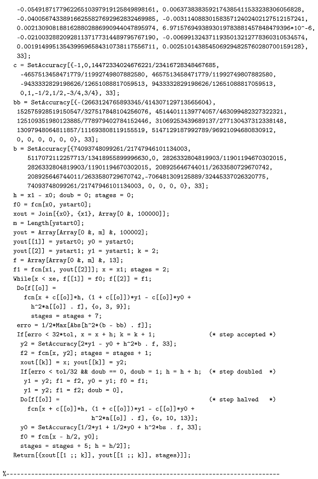
We provide a simple description of the program outlining the new implementation. In the input, we specify fcn as the function defining the problem, x0 as the initial point x 0 , x1 as the second point x 1 = x 0 + h , xe as the endpoint, ystart0 as the initial value y ( x 0 ) , ystart1 as the initial value y ( x 1 ) , tol as the tolerance τ . ystart1 approximates y ( x 0 + h ) and can be computed using a high-order Runge–Kutta method [26]. In the output, we obtain the grid in xout and the matrix containing the approximations of y at these points in yout.
It can be retrieved from http://users.uoa.gr/~tsitourasc/NumerovSol9var.m (accessed on 5 March 2025)
Mathematics 13 01257 i001Mathematics 13 01257 i002
Thus, we may verify the rightmost lower entry (i.e., for NumerovSol9var) in Figure 5 by writing the following (see [23]):
Mathematics 13 01257 i003
i.e., using less than 40,000 stages, we achieved an accuracy of almost 17 digits. The step size varied from as low as π 14000 to as large as 4 π 875 , i.e., 64 times larger. We remark here that for Arenstorf, the respective variance reaches as high as 256. This variability assisted the new variable-step method in vastly outperforming its counterpart that uses a constant step size.

References

  1. Hairer, E. Unconditionally stable methods for second order differential equations. Numer. Math. 1979, 32, 373–379. [Google Scholar] [CrossRef]
  2. Cash, J.R. High-order P-stable formulae for the numerical integration of periodic initial value problems. Numer. Math. 1981, 37, 355–370. [Google Scholar] [CrossRef]
  3. Chawla, M.M. Two-step fourth order P-stable methods for second order differential equations. BIT 1981, 21, 190–193. [Google Scholar] [CrossRef]
  4. Chawla, M.M. Numerov Made Explicit has Better Stability. BIT 1984, 24, 117–118. [Google Scholar] [CrossRef]
  5. Tsitouras, C. Explicit Numerov type methods with reduced number of stages. Comput. Maths Appl. 2003, 45, 37–42. [Google Scholar] [CrossRef]
  6. Chawla, M.M.; Rao, P.S. An explicit sixth—Order method with phase—Lag of order eight for y″ = f(t, y). J. Comput. Appl. Math. 1987, 17, 365–368. [Google Scholar] [CrossRef]
  7. Tsitouras, C. Explicit eighth order two–step methods with nine stages for integrating oscillatory problems. Int. J. Modern Phys. C 2006, 17, 861–876. [Google Scholar] [CrossRef]
  8. Franco, J.M. A class of explicit two-step hybrid methods for second-order IVPs. J. Comput. Appl. Math. 2006, 187, 41–57. [Google Scholar] [CrossRef]
  9. Franco, J.M.; Randez, R. Explicit exponentially fitted two-step hybrid methods of high order for second-order oscillatory IVPs. Appl. Maths. Comput. 2016, 273, 493–505. [Google Scholar] [CrossRef]
  10. Franco, J.M.; Randez, R. Eighth-order explicit two-step hybrid methods with symmetric nodes and weights for solving orbital and oscillatory IVPs. Int. J. Modern. Phys. C 2018, 29, 1850002. [Google Scholar] [CrossRef]
  11. Butcher, J.C. Implicit Runge Kutta processes. Math. Comput. 1964, 18, 50–64. [Google Scholar] [CrossRef]
  12. Butcher, J.C. On Runge–Kutta processes of high order. J. Austral. Math. Soc. 1964, 4, 179–194. [Google Scholar] [CrossRef]
  13. Simos, T.E.; Tsitouras, C.; Famelis, I.T. Explicit Numerov Type Methods with Constant Coefficients: A Review. Appl. Comput. Math. 2017, 16, 89–113. [Google Scholar]
  14. Coleman, J.P. Order conditions for a class of two-step methods for y″ = f(x, y). IMA J. Numer. Anal. 2003, 23, 197–220. [Google Scholar] [CrossRef]
  15. Storn, R.; Price, K. Differential evolution—A simple and efficient heuristic for global optimization over continuous spaces. J. Glob. Optim. 1997, 11, 341–359. [Google Scholar] [CrossRef]
  16. Price, K.V.; Storn, R.M.; Lampinen, J.A. Differential Evolution, A Practical Approach to Global Optimization; Springer-Verlag: Berlin/Heidelberg, Germany, 2005. [Google Scholar]
  17. Storn, R.M.; Price, K.V.; Neumaier, A.; Zandt, J.V. DeMat. Available online: https://github.com/mikeagn/DeMatDEnrand (accessed on 8 August 2024).
  18. Matlab. MATLAB Version 2018a; The MathWorks Inc.: Natick, MA, USA, 2018. [Google Scholar]
  19. Wolfram Research, Inc. Mathematica, Version 11.1; Wolfram Research, Inc.: Champaign, IL, USA, 2017. [Google Scholar]
  20. Jerbi, H.; Aoun, S.B.; Alshammari, O.; Simos, T.E.; Tsitouras, C.; Kchaou, M. On explicit ninth-order, two-step methods addressing y″ = f(x, y). Math. Meth. Appl. Sci. 2025, 48, 2517–2528. [Google Scholar] [CrossRef]
  21. Alshammari, O.; Aoun, S.B.; Kchaou, M.; Simos, T.E.; Tsitouras, C.; Jerbi, H. Eighth-Order Numerov-Type Methods Using Varying Step Length. Mathematics 2024, 12, 2294. [Google Scholar] [CrossRef]
  22. Alolyan, I.; Simos, T.E.; Tsitouras, C. Interpolants for sixth order Numerov-type methods. Math. Methods Appl. Sci. 2019, 42, 7349–7358. [Google Scholar] [CrossRef]
  23. Enright, W.; Pryce, J.D. Two FORTRAN packages for assessing initial value methods. ACM Trans. Math. Softw. 1987, 13, 1–27. [Google Scholar] [CrossRef]
  24. Arenstorf, R.F. Periodic Solutions of the Restricted Three Body Problem Representing Analytic Continuations of Keplerian Elliptic Motions. Amer. J. Maths 1963, 85, 27–35. [Google Scholar] [CrossRef]
  25. Hairer, E.; Nørsett, S.P.; Wanner, G. Solving Ordinary Differential Equations I, Nonstiff Problems, 2nd ed.; Springer-Verlag: Berlin/Heidelberg, Germany, 1993. [Google Scholar]
  26. “ExplicitRungeKutta” for NDSolve. Available online: https://reference.wolfram.com/language/tutorial/NDSolveExplicitRungeKutta.html (accessed on 8 August 2024).
Figure 1. The next step is doubled.
Mathematics 13 01257 g001
Figure 2. Abortion and halving a step.
Mathematics 13 01257 g002
Figure 3. Efficiency curves for DETEST problem D3.
Mathematics 13 01257 g003
Figure 4. Efficiency curves for DETEST problem D4.
Mathematics 13 01257 g004
Figure 5. Efficiency curves for DETEST problem D5.
Mathematics 13 01257 g005
Figure 6. Efficiency curves for Arenstorf.
Mathematics 13 01257 g006
Table 1. Number of order constraints.
Order p1234567891011
No of conditions1123610203672137275
Table 2. Equations of conditions up to the ninth order, under assumption (4).
T 1 ( 1 ) = b · 1 = 1 , T 2 ( 3 ) = b · c 2 = 1 6 , T 6 ( 5 ) = b · c 4 = 1 15 ,
b · c 6 = 1 28 , b · A 2 · c = 0 ,
b · A 3 · 1 = 1 20160 , b · A · c A c = 11 15120 ,
b · c 8 = 1 45 , b · A · c A 2 · 1 = 1 7560 ,
b · c A 2 c = 17 10080 , b · c A · c A · c = 1 720 ,
b · c A 3 · 1 = 23 60480 , b · A · 1 A 2 · c = 17 20160 ,
b · A · A · 1 A 2 1 = 1 17280 , b · c A · ( c A 2 · 1 ) = 47 181440 ,
b · A · 1 A 3 · 1 = 373 1814400 , 799 907200 = b · ( A · 1 A · ( c A · c ) ) ,
1 16200 = 1 36 b · ( c 3 A · c 3 ) , 31 181440 = b · ( c A 3 · c )
1 1814400 = b · A 4 · 1 , 1 1814400 = 1 2 b · A 3 · c 2 ,
b · A 2 · ( c A · c ) = 13 907200 , T 7 ( 9 ) = 71 907200 + b · A · ( c A 2 · c ) = 0 .
Table 3. Error conditions for the sixth-order interpolant.
1 2 · ( ρ ρ 2 ) + b ^ e ,
1 6 ρ + 1 6 ρ 3 b ^ c ^ ,
1 24 ρ 1 24 ρ 4 1 2 b ^ c ^ + b ^ A e ,
1 24 ρ 1 24 ρ 4 + 1 2 b ^ c 2 ,
1 120 ρ 1 120 ρ 5 + 1 6 b ^ c ^ + b ^ A c ^ ,
1 40 ρ 1 40 ρ 5 1 2 b ^ c 2 + b ^ ( c ^ A e ) ,
1 120 ρ + 1 120 ρ 5 1 6 b ^ c ^ 3 ,
1 720 ρ 1 720 ρ 6 1 24 b ^ c 1 2 b ^ A c ^ + b ^ A 2 e ,
1 720 ρ 1 720 ρ 6 1 24 b ^ c ^ + 1 2 b ^ A c ^ 2 ,
1 180 ρ 1 180 ρ 6 + 1 6 b ^ c ^ 2 + b ^ ( c ^ A c ^ ) ,
1 240 ρ 1 240 ρ 6 + 1 8 b ^ c 2 1 2 b ^ ( c ^ A e ) + 1 2 b ^ ( A e ) 2 ,
1 120 ρ 1 120 ρ 6 1 4 b ^ c ^ 3 + 1 2 b ^ ( c ^ 2 A e ) ,
1 720 ρ 1 720 ρ 6 + 1 24 b ^ c ^ 4 .
Disclaimer/Publisher’s Note: The statements, opinions and data contained in all publications are solely those of the individual author(s) and contributor(s) and not of MDPI and/or the editor(s). MDPI and/or the editor(s) disclaim responsibility for any injury to people or property resulting from any ideas, methods, instructions or products referred to in the content.