Transformer-Based Downside Risk Forecasting: A Data-Driven Approach with Realized Downward Semi-Variance

Abstract

Realized downward semi-variance (RDS) has been realized as a key indicator to measure the downside risk of asset prices, and the accurate prediction of RDS can effectively guide traders’ investment behavior and avoid the impact of market fluctuations caused by price declines. In this paper, the RDS rolling prediction performance of the traditional econometric model, machine learning model, and deep learning model is discussed in combination with various relevant influencing factors, and the sensitivity analysis is further carried out with the rolling window length, prediction length, and a variety of evaluation methods. In addition, due to the characteristics of RDS, such as aggregation and jumping, this paper further discusses the robustness of the model under the impact of external events, the influence of emotional factors on the prediction accuracy of the model, and the results and analysis of the hybrid model. The empirical results show that (1) when the rolling window is set to 20, the overall prediction effect of the model in this paper is the best. Taking the Transformer model under SSE as an example, compared with the prediction results under the rolling window length of 5, 10, and 30, the RMSE improvement ratio reaches 24.69%, 15.90%, and 43.60%, respectively. (2) The multivariable Transformer model shows a better forecasting effect. Compared with traditional econometric, machine learning, and deep learning models, the average increase percentage of RMSE, MAE, MAPE, SMAPE, MBE, and SD indicators is 52.23%, 20.03%, 62.33%, 60.33%, 37.57%, and 18.70%, respectively. (3) In multi-step prediction scenarios, the DM test statistic of the Transformer model is significantly positive, and the prediction accuracy of the Transformer model remains stable as the number of prediction steps increases. (4) Under the impact of external events of COVID-19, the Transformer model has stability, and the addition of emotional factors can effectively improve the prediction accuracy. In addition, the model’s prediction performance and generalization ability can be further improved by stacked prediction models. An in-depth study of RDS forecasting is of great value to capture the characteristics of downside risks, enrich the financial risk measurement system, and better evaluate potential losses.

1. Introduction

Research on financial market risk plays an important role in understanding the operating mechanism of the financial market, improving the financial theoretical system, evaluating and managing investment risks, etc. Volatility is an indicator that measures the range and frequency of market price changes over a period of time, reflecting the uncertainty of financial asset prices and the risk of asset investment [1]. Although volatility is a common risk measure, it measures both the upward and downward movements of asset prices. However, investors generally pay more attention to the potential losses caused by falling asset prices, known as downside risk. Therefore, the research on downside risk, especially the prediction accuracy of the downside risk measurement index, also known as realized downward semi-variance (RDS), is of great significance to help investors reduce extreme losses and assist financial institutions in effectively evaluating risk management strategies.

According to whether various factors of the market are included, volatility prediction models are divided into autoregressive models and multiple regression models. The autoregressive model realizes reasonable prediction by capturing the features of volatility itself. Early scholars estimated and predicted volatility under low-frequency data through traditional econometric models, such as the autoregressive conditional heteroskedasticity (ARCH) model [2], the generalized autoregressive conditional heteroskedasticity (GARCH) model [3], and stochastic volatility (SV) model [4]. These models can extract the linear and deterministic information and save the uncertain information in the residual sequence. However, it usually needs to satisfy the assumptions of a linear relationship, stationarity, a normal distribution, etc., so it has obvious shortcomings when dealing with complex nonlinear high-dimensional data. With the continuous improvement of the accessibility of high-frequency data, its rich intraday feature information is gradually mined and utilized, and many scholars consider increasing the modeling frequency down to the day and minute. Andersen and Bollerslev [5] proposed realized volatility (RV) and provided a method to estimate volatility directly from intraday high-frequency data by calculating the cumulative square daily return under high-frequency data. Thus, the potential unobservability of volatility and the estimation of conditional variance can be effectively solved. Classical RV models include the autoregressive fractionally integrated moving average-RV (ARFIMA-RV) model proposed by Andersen et al. [6] and the heterogeneous autoregressive-RV (HAR-RV) model proposed by Corsi [7], which characterized the autocorrelation and long memory characteristics of RV to achieve effective prediction. Izzeldin et al. [8], Liang et al. [9], and Korkusuz et al. [10] forecast multi-market and multi-stock RV based on the HAR model, the HAR-RV-Average model, and the HAR-RV-X framework, respectively.

Although the traditional econometric model can describe the volatility aggregation characteristics and has the advantages of clear statistical principle, strong explanation, clear structure, and stable parameters, the model has strict requirements on assumptions such as data distribution, which makes it difficult to fully capture the nonlinear relationship in the time series, and has high processing cost and limited prediction accuracy. Therefore, machine learning models, which are good at capturing complex nonlinear relationships and extracting high-dimensional data features, are widely used to predict RV in financial markets with non-stationary, nonlinear, aggregated, and jumping characteristics. For example, Fałdziński et al. [11] applied support vector regression (SVR) to predict the volatility of energy commodity futures contracts such as crude oil and natural gas. Compared with the single machine learning model with outlier sensitivity and weak generalization ability, the ensemble machine learning model achieves a more robust prediction model by combining multiple weak learners. For example, Luong and Dokuchaev [12] and Demirer et al. [13] used RF models to forecast the RV of the stock index and crude oil, respectively. However, the ensemble learning model still needs a lot of feature engineering work, and the ability to process high-dimensional complex structure data needs to be improved. Compared to the ensemble learning model, the deep learning model approximates complex nonlinear features infinitely using multi-layer nonlinear transformation and has strong automatic feature learning and generalization ability. Traditional deep learning models, such as long short-term memory (LSTM) and the gated recurrent unit (GRU), have been widely used to predict financial stock market volatility [14,15,16].

The trend and fluctuation of the financial stock market are easily affected by company fundamentals, macroeconomic factors, market sentiment, and other aspects. Multiple regression methods can consider multiple influencing factors at the same time, conduct a comprehensive analysis of the financial market, extract relevant features, and accurately understand market dynamics. Some scholars use multivariate regression models to forecast RV in the stock market. For example, Todorova and Souček [17] incorporated overnight information flow into the RV prediction of ASX 200 and seven highly liquid Australian stocks. Audrino et al. [18] made use of a large amount of emotion and search information on the website, combined with emotion classification technology, an attention mechanism, and the high-dimensional predictive regression model, to predict volatility. Kim and Baek [19] proposed the FAHAR-LSTM model, which incorporated multiple relevant transnational stock market volatility information into the RV prediction of the Asian stock market. Kambouroudis et al. [20] extended implied volatility (IV), the leverage effect, and overnight returns into the HAR and predicted the RV of 10 international stock indexes. Lei et al. [21] used the LSTM model to forecast stock RV by taking trading information, on-floor trading sentiment, and unstructured forum text information as input variables. Jiao et al. [22] took trading information and news text information in the crude oil market as input variables and used the LSTM to forecast the RV of crude oil. Ma et al. [23] proposed a parallel neural network model of CNN-LSTM and LSTM based on mixing big data, which considered a variety of micro and macro variables and processed mixed frequency data through the RR-MIDAS model. Zhang et al. [24] introduced transaction information and sentiment indicators into the LSTM model, combined with the jump decomposition method, to predict RV.

There are two shortcomings in the existing literature. First, most of the target variables for prediction focus on RV, which is used as an indicator to measure risk. RV is calculated by the sum of the squares of the intraday high-frequency logarithmic returns, so falls and rises in stock prices have the same effect on RV, but it should be noted that there is significant leverage in the market, and the distribution of returns is asymmetric. Granger [25] points out that the risk of an investment is mainly related to low or even negative returns. In reality, investors tend to be more sensitive to investment losses, and the left tail of the return distribution constitutes a downside risk, which can better reflect investors’ concern about trading losses. However, RV ignores the effect of leverage on stock market transactions in the calculation process, making it difficult to reflect investors’ concerns about downside risks. Barndorff-Nielsen et al. [26] proposed the RDS based on the high-frequency negative return rate. Therefore, this paper takes high-frequency RDS, which is more concerned with the market, as the forecast object and fully studies the amplitude and frequency of downward fluctuations of asset prices.

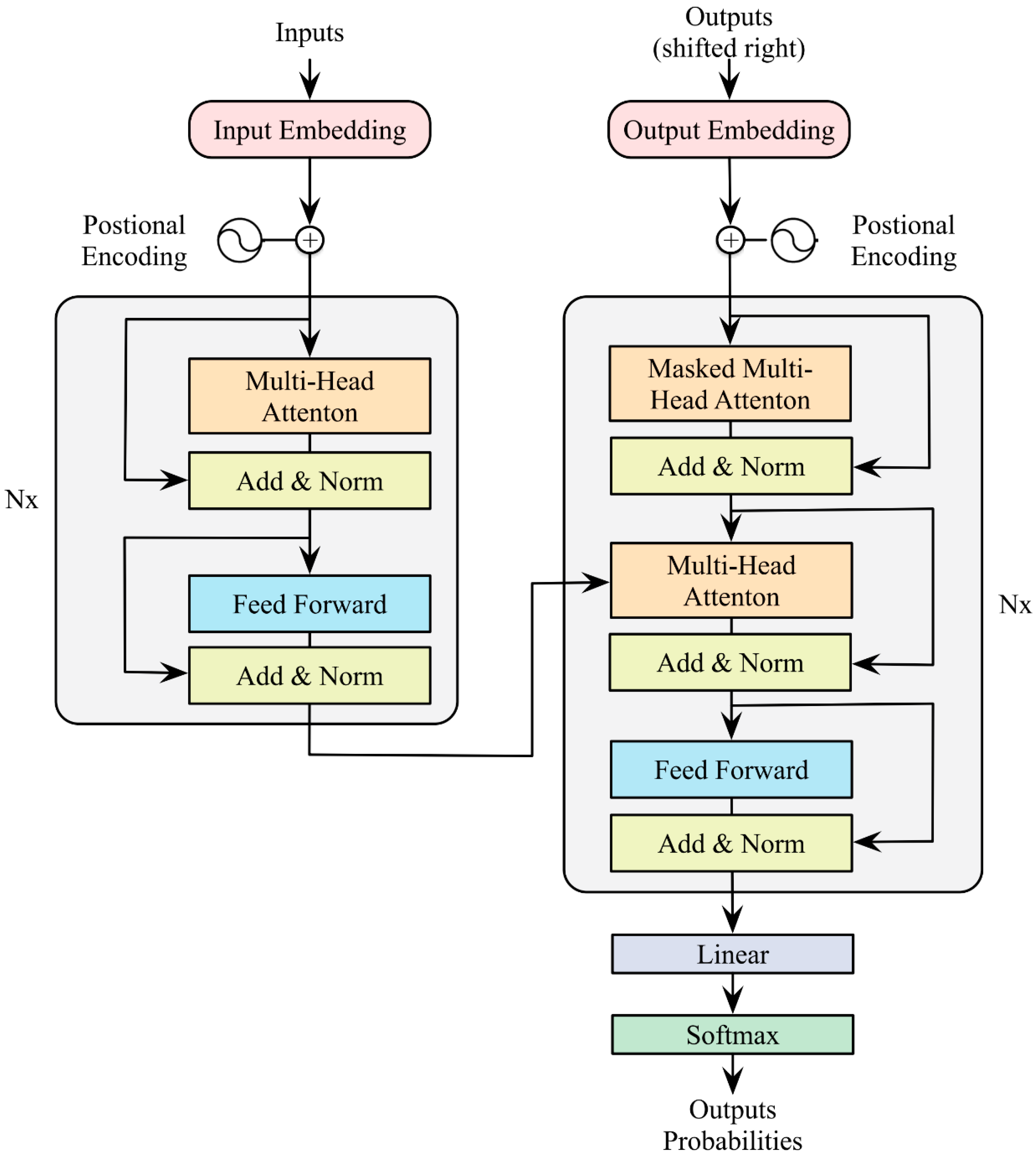
In addition, from the perspective of volatility prediction models, most studies use traditional deep learning models (RNN, LSTM, and GRU) to predict volatility. According to the descriptive statistical analysis below, it can be found that RDS has a strong long-term autocorrelation, but the traditional deep learning model cannot capture global information and deal with long-distance dependencies in long sequences. Therefore, this paper adopts a new deep learning model called Transformer, which abandons the cyclic structure of recurrent neural networks (RNNs) and uses self-attention mechanisms and parallel computation to process sequential data. The model is not only good at capturing global information and long-term dependencies but is also able to capture ultra-short-term feature changes, which is suitable for RDS data with long-term autocorrelations and short-term aggregation jumps.

To sum up, compared with the existing literature, this study is more in line with the downside risk indicator RDS of investors’ risk preference. Multiple factor variables related to RDS, including market trading information, floor trading sentiment, the volatility of trading indicators, etc., are selected to study the correlation between various influencing factors and RDS. Secondly, the downside risk measure RDS is predicted and analyzed using a multivariable Transformer prediction model that is good at capturing global information and short-term characteristics. Finally, various evaluation criteria and the DM test are used to analyze the sensitivity of scroll window size, prediction step size, and prediction model performance. The robustness of the model under structural fracture, the influence of the emotion index on model prediction, and the RDS prediction results under the stacked-ML-DL framework are discussed.

The marginal contribution of this paper mainly includes the following three points:

(1)

Predict objects: Compared with the existing literature, the research objective of this paper focuses on downside risk measurement, also known as RDS prediction based on high-frequency data. The downside risk is consistent with investors’ risk preference, which describes the potential loss of the portfolio. The study of downside risk measurement RDS is conducive to further distinguishing the impact of different price changes on market risk and traders’ behavior and more accurately capturing the negative volatility characteristics of assets, thus helping traders avoid possible major losses when the market falls and optimize the investment portfolio to achieve more robust investment returns.

(2)

Prediction model: In this paper, combined with multiple market influencing factors such as trading volume, trading volume volatility, overnight information, turnover rate, and moving average, Transformer is used to forecast RDS. Compared to traditional deep learning LSTM and GRU models, the Transformer model uses a self-attention mechanism to simultaneously process global data, which is better able to capture long-distance dependencies when processing the long series data. In addition, the model abandons serialization processing and makes full use of the advantages of parallel computing to effectively improve the model’s training and operation efficiency. By inputting a variety of relevant variables into the Transformer model, its high computation and strong long-range capture capability can be used to improve the prediction accuracy and efficiency of RDS. In addition, the predictive effects of the ML and DL stack models are discussed and compared with the single Transformer model.

(3)

Sensitivity analysis: In this paper, a variety of evaluation criteria and improvement ratios are used to explore the impact of the size of each model’s rolling window on the prediction accuracy under one-step prediction. In addition, by studying the evaluation criteria results of each model under different prediction lengths, the robustness of each model is analyzed and tested. Combined with evaluation criteria and the DM test, the results of one-step prediction and multi-step prediction among different models are compared, and the accuracy and robustness of the Transformer model in RDS prediction are comprehensively tested through event shock and emotion factor analysis.

The research content of this paper is to construct a Transformer multivariable model to predict the RDS and analyze the empirical results. The remainder of this article is structured as follows: Section 2 defines RDS and introduces the Transformer model and prediction evaluation methods. In Section 3, multivariate rolling prediction is carried out by combining nine forecasting variables, demonstrating the empirical results of various multivariate forecasting models, and using a variety of evaluation criteria, the DM test, and other methods to analyze the sensitivity of the rolling window length, prediction length, and prediction model to give the optimal model. Section 4 discusses the robustness of the model under event shock and the influence and effect of adding an emotion index on the RDS prediction models. Section 5 explores the forecasting performance of the stacked-ML-DL hybrid forecasting framework and provides empirical analysis. Section 6 summarizes the content of the paper and provides its limitations and future extension.

2. Theoretical Basis

2.1. Realized Downward Semi-Variance (RDS)

Barndorff-Nielsen et al. [26] proposed RDS based on the high-frequency negative rate of return, which has become an indicator in the financial field to measure the downside risk of financial assets or investment portfolios. Unlike the traditional RV, RDS only focuses on the volatility of the asset price with a negative yield, and the semi-variance measure achieved using high-frequency intraday data provides a deeper understanding of the risk characteristics of the asset, especially during periods of market stress. Therefore, RDS is considered to be a more accurate risk measurement for stocks and other assets in the case of market declines, especially for those investors who are only concerned about the risk of asset values falling.

Under the risk-free arbitrage hypothesis, the logarithmic asset price process follows the semi-martingale process. Suppose that logarithmic asset price processes ${\left(X_t\right)}_{t⩾0}$ defined on the filtered probability space $\left(\mathrm{\Omega },\mathcal{F},{\left({\mathcal{F}}_t\right)}_t⩾0,P\right)$ are Itô semi-martingale processes, which have the following form:

$$\begin{array}{ll}{X}_t=& X_0+{\int }_0^t{a}_s\mathrm{d}s+{\int }_0^t{\sigma }_s\mathrm{d}{W}_s+{\int }_0^t{\int }_{\left|x\right|<1}\kappa \circ \delta \left(s,x\right)\left(\mu -\nu \right)\left(\mathrm{d}s,\mathrm{d}x\right)\\ & +{\int }_0^t{\int }_{\left|x\right|⩾1}{\kappa }^{\prime }\cdot \delta \left(s,x\right)\mu \left(\mathrm{d}s,\mathrm{d}x\right),\end{array}$$

(1)

where $W$ is a standard Brownian motion, ${\left(a_s\right)}_{s⩾0}$ is a locally bounded predictable drift process, and ${\left({\sigma }_s\right)}_{s⩾0}$ is a volatility process. $\delta (\omega ,t,x)$ is a predictable càglàd function satisfying that ${\mathrm{s}\mathrm{u}\mathrm{p}}_{x\in E}{\displaystyle \frac{\left|\delta \right(\omega ,t,x\left)\right|}{\gamma \left(x\right)}}$ is locally bounded, where $\gamma$ is a nonnegative function ($E$ is a subset of $\mathbb{R}$). $\mu$ is a Poisson random measure on $\mathbb{R}+\times E$ with the intensity measure $\nu (\mathrm{d}s,\mathrm{d}x)=\mathrm{d}s\otimes \lambda \left(\mathrm{d}x\right)$. In addition, $\kappa$ is a continuous truncation function and is bounded on the compact support set.

In practice, only discrete data such as transaction prices can be observed in financial markets. Therefore, based on the high-frequency discrete observation point data of intraday asset price $X_t$ at a given time $T$, RDS can be defined as

$$\mathrm{R}\mathrm{D}\mathrm{S}\left(t\right)=\sum _{i=1}^{{\displaystyle \frac{1}{\Delta }}}{r}_{t,i}^2{I}_{\left\{r_{t,i}\le 0\right\}},t=0,\dots ,T,$$

(2)

where $\Delta$ is the sample interval, $1/\Delta$ is the number of samples, $r_{t,i}=ln\left(X_{t-1+\Delta i}\right)-ln\left(X_{t-1+\Delta \left(i-1\right)}\right.)$, and $I_x$ is the indicative function, whereby the value is 1 when {∙} is true and 0 when {∙} is false.

2.2. Transformer Model

Transformer is a self-attentional deep learning model originally proposed by Vaswani et al. [27] to solve sequence modeling tasks in natural language processing (NLP). However, due to its excellent performance in processing time series data, Transformer has also been widely used in financial time series analysis in recent years, such as predicting realized volatility. The Transformer model is mainly composed of two parts: the encoder and the decoder, and in time series prediction tasks, we usually only need the encoder part. Encoders capture complex dependencies between data through multiple stacked hierarchies.

The overall structure of the Transformer model depicted in Figure 1 can be summarized as the alternating stacking of self-attention modules and feedforward neural network modules. Each layer contains two key components: the multi-head self-attention mechanism and the feedforward neural network.

In Figure 1, the input is entered into the encoder after the positional encoding and embedding layer. The encoder consists of several stacked layers, each consisting of a self-attention module and a feedforward neural network module.

(1)

Self-Attention Mechanism

The core of the self-attention mechanism is to assign different weights to each element in the sequence to capture global context information. For the input sequence $X\in R^{n\times d}$ (where $n$ is the number of time steps and $d$ is the feature dimension), the steps for calculating self-attention are as follows:

Step 1. Calculate the query vector, key vector, and value vector:

$$Q=X{W}^Q,K=X{W}^K,V=X{W}^V,$$

(3)

where $W^Q$, $W^K$, and $W^V$ are weight matrices of the query, key, and value, respectively.

Step 2. Calculate the attention score:

$$A=\mathrm{softmax}\left({\displaystyle \frac{Q{K}^T}{\sqrt{d_k}}}\right),$$

(4)

where $d_k$ is the dimension of the key vector used for scaling so that the dot product remains in the appropriate range of values.

Step 3. Generate the output:

$$Z=AV.$$

(5)

Multi-head self-attention mechanisms are extensions of self-attention mechanisms that enhance the learning ability by executing multiple attention mechanisms in parallel and then stitching together the respective outputs. The formula for the self-attention of bulls is

$$\mathrm{MultiHead}\left(Q,K,V\right)=\mathrm{Concat}\left({\mathrm{head}}_1,\dots ,{\mathrm{head}}_{\mathrm{h}}\right)W^O,$$

(6)

where $\mathrm{h}$ indicates the use of h parallel attention heads. The output of each attentional head is

$${\mathrm{head}}_{\mathrm{i}}=\mathrm{Attention}\left(X{W}_i^Q,X{W}_i^K,X{W}_i^V\right).$$

(7)

Since the Transformer model lacks timing awareness, timing information needs to be injected through location coding. This paper adopts sinusoidal coding:

$$P{E}_{\left(pos,2i\right)}=\sin \left({\displaystyle \frac{ \mathrm{pos} }{{10000}^{\frac{2i}{d}}}}\right),$$

(8)

$$P{E}_{\left(pos,2i+1\right)}=\cos \left({\displaystyle \frac{ \mathrm{pos} }{{10000}^{\frac{2i}{d}}}}\right),$$

(9)

where $pos$ is the time step position and $i$ is the dimension index. The encoding results are added to the input features and fed into the model.

(2)

Feedforward Neural Network

The part of the feedforward neural network consists of two fully connected layers and usually uses the activation function $\mathrm{R}\mathrm{e}\mathrm{L}\mathrm{U}$ in the middle. Feedforward networks can be represented as

$$\mathrm{FFN}\left(x\right)=\mathrm{ReLU}\left(x{W}_1+b_1\right)W_2+b_2.$$

(10)

(3)

Residual Connection and Layer Normalization

To mitigate the gradient loss problem, each sublayer in the Transformer model (i.e., the self-attention layer and the feedforward layer) introduces residual connectivity and layer normalization:

$$\mathrm{LayerNorm}\left(x+\mathrm{Sublayer}\left(x\right)\right).$$

(11)

This structure contributes to the effective transmission of information and improves the training efficiency of the model.

In the downward volatility prediction task achieved in this paper, the input sequence $X\in R^{n\times d}$ contains $d$-dimensional features of $n$ historical time steps, $d$-dimensional embedding is obtained via linear projection, and multi-scale timing features are extracted by stacking $N$ encoder layers. Finally, the predicted values of $T$ future time steps are output through the fully connected layer:

$$\widehat{Y}=W_h{H}^{\left(N\right)}+b_h,$$

(12)

where $H^{\left(N\right)}$ is the top-level encoder output and $W_h\in {\mathbb{R}}^{T\times d}$ is the prediction weight matrix.

2.3. Evaluation Index

2.3.1. Loss Evaluation Criteria

In this paper, the mean absolute percentage error (MAPE), root mean square error (RMSE), mean absolute error (MAE), symmetric mean absolute percentage error (SMAPE), mean bias error (MBE), and standard deviation (SD) are used to evaluate and compare the error sequences of each model [28,29]. The calculation method is as follows:

$$\mathrm{M}\mathrm{A}\mathrm{P}\mathrm{E}={\displaystyle \frac{1}{N}}\sum _{n=1}^N{\displaystyle \frac{\left|{\widehat{y}}_n-y_n\right|}{y_n}},$$

(13)

$$\mathrm{R}\mathrm{M}\mathrm{S}\mathrm{E}=\sqrt{{\displaystyle \frac{1}{N}}\sum _{n=1}^N{\left({\widehat{y}}_n-y_n\right)}^2},$$

(14)

$$\mathrm{MAE}={\displaystyle \frac{1}{N}}\sum _{n=1}^N\left|{\widehat{y}}_n-y_n\right|,$$

(15)

$$\mathrm{S}\mathrm{M}\mathrm{A}\mathrm{P}\mathrm{E}={\displaystyle \frac{1}{N}}\sum _{n=1}^N{\displaystyle \frac{\left|{\widehat{y}}_n-y_n\right|}{(\left|{\widehat{y}}_n\right|+\left|y_n\right|)/2}},$$

(16)

$$\mathrm{M}\mathrm{BE}={\displaystyle \frac{1}{N}}\sum _{n=1}^N({\widehat{y}}_n-y_n),$$

(17)

$$\mathrm{SD}=\sqrt{{\displaystyle \frac{\sum _{n=1}^N{\left({\widehat{y}}_n-Arithmetic mean\right)}^2}{total number}}},$$

(18)

where $y_n$ indicates the true value and ${\widehat{y}}_n$ indicates the predicted value.

2.3.2. DM Test

The Diebold–Mariano test (DM test) [30] is a method used to compare the two time series prediction models to check whether there are significant differences in the prediction errors of different models to determine which model has better prediction results. The DM test is a statistical significance test based on the average difference in prediction errors. Assuming two models make predictions throughout $T$, the error sequence of model $\alpha$ and model $\beta$ can be expressed as

$$E_{\alpha }=\left\{f\left(y_1^{\alpha },\widehat{y_1^{\alpha }}\right),f\left(y_2^{\alpha },\widehat{y_2^{\alpha }}\right),\dots ,f\left(y_T^{\alpha },\widehat{y_T^{\alpha }}\right)\right\},$$

(19)

$$E_{\beta }=\left\{f\left(y_1^{\beta },\widehat{y_1^{\beta }}\right),f\left(y_2^{\beta },\widehat{y_2^{\beta }}\right),\dots ,f\left(y_T^{\beta },\widehat{y_T^{\beta }}\right)\right\},$$

(20)

where $f\left(·\right)$ represents the error function (MAPE is adopted in this paper); $y$ and $\widehat{y}$ represent the real value and predicted value, respectively; the superscript represents the model; and the subscript represents the sequence length.

DM statistics can be calculated as follows:

$$DM={\displaystyle \frac{\overline{D}}{\sqrt{\frac{\sum _{i=1}^T{\left(d_i-\overline{D}\right)}^2}{T-1}}}}\to N\left(\mathrm{0,1}\right),$$

(21)

where $D=E_{\alpha }-E_{\beta }=\left\{d_1,d_2,\dots ,d_T\right\}$, $\overline{D}={\displaystyle \frac{\sum _{i=1}^{\mathrm{T}}{\mathrm{d}}_{\mathrm{i}}}{T}}$, and DM test statistics follows the standard normal distribution $N\left(\mathrm{0,1}\right)$. The null hypothesis and alternative hypothesis related to DM in this paper are as follows:

$H_0$: when $\left|DM\right|=0$, it indicates that the predictive performance of the two models is the same;

$H_1$: when $\left|DM\right|\ne 0$, it indicates that there is a difference in the performance of these two models.

If $DM$< 0, it indicates that model A has a better forecasting ability than model B; otherwise, it indicates that model B has a better forecasting ability than model A. The more significant the difference between the models, the greater the value of $\left|DM\right|$.

3. Empirical Results

3.1. Data Sources and Variables

This paper selects the Shanghai Stock Exchange (SSE) stock index from 17 February 2011 to 31 October 2022 (2846 days in total) as the analysis object and obtains 48 high-frequency trading data every day with 5 min as the sampling frequency. The daily RDS is calculated using the negative return rate portion of the adjacent 5 min. To discuss the RDS volatility levels of the SSE, Figure 2 shows the RDS chart, which is calculated using the SSE over the study year, and shows the external event shocks corresponding to the time when the RDS produces sharp fluctuations. Overall, the sharp fluctuations of RDS can usually correspond to some external event shocks, including macroeconomic situations, international trade relations, government policy adjustments, geopolitical conflicts, world epidemic impacts, trading market sentiment, etc. Observing the SSE, it is found that the downside risk of the stock index has increased sharply around 2015 and 2020, and the RDS has fluctuated significantly. The specific reasons for the fluctuations are as follows: in 2015, the global market fluctuated sharply due to events and factors such as the expected interest rate hike of the Federal Reserve, the liquidation of leveraged funds, geopolitical tensions, and market panic; the year 2020 was hit hard by the COVID-19 pandemic.

Therefore, studying the changes in the level of RDS plays an important role in studying the downside risk of the market. The accurate prediction of RDS can help investors quickly adjust their trading strategies in the face of global shocks, thereby reducing investment risks. In the fourth chapter, this paper selects COVID-19 to deeply study the robustness of the forecast model. At the time of the outbreak, market panic spread, and investors were pessimistic about future economic growth expectations, leading to rapid declines in global stock markets. By analyzing the influence of market panic and other emotional factors, the impact of the change in investor sentiment on the stock market and downside risk indicators is further discussed. The study of external shocks and emotional factors helps to evaluate the performance of the model under extreme market conditions and also provides a theoretical basis for investors to adjust their strategies in similar crises.

In addition, by using the access and computing of nine associated variables like trading information and investors’ emotions as the predictor variables of RDS prediction, all variable data are taken from the JoinQuant database (URL: https://www.joinquant.com (accessed on 31 December 2024)). The meanings of specific variables are shown in

Table 1. Specific explanations of predictor variables.

Variables	Explanation
Volume	The number of transactions between the buyers and sellers of stocks in a given period. It is usually measured by the number of shares traded and the amount of transactions, which can reflect the market activity.
Bias	A measure of the gap between stock prices and moving averages. It is used to assess whether a stock price is too high or too low and may be similar to the moving average trend.
DMA	An indicator that assesses the power of buyers and sellers and future price movements, and it is derived from the difference between the moving averages of two different cycles.
CDP	Contrarian operating system. It is mainly used for short-term transactions, reflecting the relationship between the highest price, the lowest price, and the closing price in the market.
AR	Indicators of market sentiment. AR measures the strength of buying and selling in the market; a high AR value indicates strong buying, while a low AR value indicates strong selling.
BR	A buyer’s ratio. As an indicator of the market’s desire to buy and sell, an increase in BR indicates the buyer’s strength, while a decrease in BR indicates the seller’s strength.
OI	Overnight information, that is, market information accumulated during non-trading hours. It can often affect the market opening and trading behavior of the next trading day.
RV-V	Volatility of trading volume. It reflects the degree of change in market trading volume.
CR	Change rate. It is a measure of how much a price has changed over a given period.

. For variable selection and calculation formulas, refer to Lei et al. [21].

Figure 3 shows the Spearman correlation coefficient results among various related influencing factors under SSE. As can be seen from Figure 3, the correlation coefficient between volume and RDS is the highest, reaching a positive value of 0.41, which means that volume and RDS have a significant positive correlation, indicating that the transmission of new information will affect the market price fluctuation and trading volume at the same time, and traders often choose to trade when the market is active. On the contrary, bias, CR, and DMA are negatively correlated with RDS. The correlation between the covariance tests of each influence index is generally low, indicating that introducing these variables into the model at the same time will not cause serious multicollinearity problems.

In the case of SSE,

Table 2. Descriptive statistics of RDS and predictor variables of SSE.

SSE	RDS	Volume	Bias	DMA	CDP	AR	BR	OI	RV-V	CR
Mean	0.544	2.137 × 1010	1.410 × 104	1.422 × 10−1	2.919 × 103	6.788	8.843	−2.963	3.334	8.100 × 105
Standard deviation	1.254	1.329 × 1010	1.956 × 102	4.010 × 10−1	5.454 × 102	6.686 × 101	8.832 × 101	1.918 × 101	3.477 × 101	1.298 × 102
Min	1.808 × 10−2	3.963 × 109	−1.729 × 101	−3.472 × 102	1.933 × 103	−1.000	0.000	−2.598 × 102	6.684 × 10−1	−8.490 × 102
Max	1.868 × 10−1	8.571 × 1010	9.520 × 102	2.019 × 102	5.154 × 103	2.164 × 103	3.722	2.883 × 102	1.362 × 103	5.760 × 102
Skewness	7.927	1.253	−9.379 × 10−1	−1.514	2.299 × 10−1	2.477 × 101	3.092 × 101	−2.236	3.772 × 101	7.932 × 10−1
Kurtosis	8.166 × 101	1.669	6.704	1.197 × 10−1	3.189 × 10−1	7.024 × 102	1.170 × 103	5.538 × 101	1.426 × 103	6.212
Jarque–Bera	8.177 × 105 **	1.072 × 103 **	5.724 × 103 **	1.800 × 104 **	3.690 × 101 **	5.859 × 107 **	1.623 × 108 **	3.647 × 105 **	2.408 × 108 **	4.854 × 103 **
ADF	−5.098 ***	−3.707 ***	−9.665 ***	−8.393 ***	−2.242	−5.330 × 101 ***	−5.355 × 101	−7.046 × 101 ***	−9.130 ***	−9.612 ***
Q (5)	3.973 × 103 **	1.307 × 104 **	2.459 × 103 **	6.379 × 103 **	1.402 × 104 **	2.350 × 10−1 **	9.082 × 10−1 **	4.109 × 101 **	7.114 × 102 **	8.463 **
Q (10)	5.839 × 103 **	2.273 × 104 **	2.469 × 103 **	6.489 × 103 **	2.760 × 104 **	4.334 × 10−1 **	9.731 × 10−1 **	7.970 × 101 **	7.114 × 102 **	3.091 × 101 **
Q (20)	9.534 × 103 **	4.135 × 104 **	2.508 × 103 **	6.515 × 103 **	5.342 × 104 **	8.882 × 10−1 **	1.374 **	1.483 × 102 **	7.117 × 102 **	6.240 × 101 **

Note: The symbols ** and *** signify the rejection of the null hypothesis at significance levels of 5% and 1%, respectively. The Jarque–Bera test assesses whether the dataset conforms to a normal distribution. The stationarity of the time series is evaluated using the augmented Dickey–Fuller (ADF) test. Q (n) denotes the Ljung–Box Q statistic, with n indicating the lag order, which tests if the sequence data behave as white noise.

shows descriptive statistics for RDS and various predictors. From the perspective of the skewness value, most variables are high, indicating that the data distribution is not completely symmetric, with obvious left or right skewness. For example, the skewness of OI is −2.236, which is much less than 1, meaning that the distribution may be skewed to the left. The skewness values of AR, BR, and RV-V are all greater than 10, indicating that the distribution may be significantly skewed to the right. From the perspective of the kurtosis value, while the volume and CDP are less than three, the other variables are much higher than the critical value of three; that is, the distribution of data is sharper than the normal distribution, and there are more extreme values. The Jarque–Bera test results show that at the significance level of 5%, the null hypothesis that each variable sequence is normally distributed is rejected. The results of the ADF stationarity test show that when the significance level is 1%, except for the CDP index, the t statistics of all other sequences are smaller than the critical ADF test value, failing the unit root test, and the data have non-stationarity characteristics. At the same time, for Q statistics with a lag of 5, 10, and 20, the null hypothesis that the corresponding order has no autocorrelation is rejected at the significance level of 5%, which reflects the characteristics of the long memory of the sequence.

3.2. Data Preprocessing and Rolling Prediction

Due to the different scales between variables, the direct use of raw data can lead to certain large-scale features dominating the model, affecting the stability and convergence rate of machine learning and deep learning models. Therefore, this paper uses the min–max normalization algorithm to preprocess data and scale the data to the interval $\left[\mathrm{0,1}\right]$ through linear transformation. The calculation formula is as follows:

$$x_i^{\prime }={\displaystyle \frac{x_i-\mathrm{m}\mathrm{i}\mathrm{n}\left(x\right)}{\mathrm{m}\mathrm{a}\mathrm{x}\left(x\right)-\mathrm{m}\mathrm{i}\mathrm{n}\left(x\right)}},i=\mathrm{1,2},\cdots ,n,$$

(22)

where $x_i$ is the original data point; $\mathrm{m}\mathrm{i}\mathrm{n}\left(x\right)$ and $\mathrm{m}\mathrm{a}\mathrm{x}\left(x\right)$ are the minimum and maximum values in dataset $x$, respectively; and $x_i^{\prime }$ is the normalized data point.

To capture new trends and patterns in the data in time, this paper selects the rolling prediction method to predict the RDS value of the next day by rolling the historical data of the past L days, as shown in Figure 4. The rolling forecasting approach is more closely aligned with the latest market trends and conditions, allowing the model to use the latest data at each forecast step to maintain accuracy and relevance. In this paper, L is selected as 5, 10, 20, and 30, respectively. By comparing the prediction states and capabilities under different rolling windows, the optimal rolling window can be determined and applied to all prediction models.

3.3. One-Step Prediction Result

In this study, all models and tests are run on Python3.10 on a computer with a 1.60 GHz CPU and 16 GB of memory. In this paper, seven different predictive models are used, including the traditional econometric model (Ridge regression), the single machine learning model (SVR), the ensemble machine learning model (RF, XGBoost 3.0.0), the traditional deep learning model (LSTM, GRU), and the novel deep learning model (Transformer). To investigate the influence of historical data length on the roll prediction model and compare the performance of various models on the SSE dataset, this section will use four different rolling window sizes (5, 10, 20, and 30) to make a one-step prediction of RDS. Under different rolling windows, the results of the one-step prediction evaluation criteria of RDS of SSE are shown in

Table 3. Six evaluation criteria for the one-step prediction of different prediction models under different rolling windows of SSE.

Model	History_Length = 5						History_Length = 10
	RMSE	MAE	MAPE	SMAPE	MBE	SD	RMSE	MAE	MAPE	SMAPE	MBE	SD
Ridge	0.8514	0.7990	5.0727	1.1949	0.7750	0.3582	0.8653	0.8092	5.1277	1.1978	0.7944	0.3442
SVR	1.1907	0.7373	4.1167	1.0852	0.4832	1.0928	0.7576	0.4812	2.5972	1.1263	0.0495	0.7481
RF	0.9473	0.7456	4.7750	1.0309	0.7063	0.6361	0.9392	0.7534	4.6780	1.0629	0.7232	0.6010
XGBoost	0.7077	0.4577	2.5946	0.8785	0.3161	0.6359	0.8979	0.5529	2.7555	1.0121	0.3433	0.8280
LSTM	0.5471	0.3577	1.5460	0.6643	0.1786	0.5171	0.5995	0.4578	2.7116	0.9153	0.3624	0.4775
GRU	0.6302	0.5901	3.9589	1.0769	0.5261	0.3469	0.7010	0.6584	4.5120	1.1221	0.5959	0.3693
Transformer	0.4131	0.3424	2.2978	0.8372	−0.3080	0.3551	0.3699	0.2003	0.6233	0.6033	−0.3218	0.3394
Model	History_Length = 20						History_Length = 30
	RMSE	MAE	MAPE	SMAPE	MBE	SD	RMSE	MAE	MAPE	SMAPE	MBE	SD
Ridge	0.8411	0.7845	4.9655	1.1831	0.7697	0.3343	0.8154	0.7575	4.8068	1.1676	0.7352	0.3789
SVR	0.6845	0.4816	2.7548	1.0474	0.2336	0.5983	0.6895	0.5376	3.3503	1.1015	0.3264	0.5982
RF	0.7450	0.6201	4.1044	1.0161	0.5684	0.4702	0.7874	0.6284	4.1953	0.9876	0.5864	0.5481
XGBoost	0.6809	0.5647	3.6178	1.0267	0.4961	0.3314	0.7040	0.4187	2.1538	0.8259	0.2600	0.6638
LSTM	0.4392	0.3472	2.1610	0.8157	0.2714	0.3453	0.6239	0.5359	3.3823	1.0071	0.4605	0.4393
GRU	0.6018	0.4623	1.7210	1.8165	0.4057	0.2909	0.5758	0.4965	2.1267	2.0000	−0.5230	0.3618
Transformer	0.3111	0.1930	0.9888	0.6056	−0.1719	0.3212	0.5516	0.5169	3.6497	1.0424	−0.2931	0.3616

Note: The number underlined in bold indicates the optimal value under the column criteria.

. To more intuitively present the specific impact of various lengths of historical information on the prediction accuracy of each model, as well as the changing trend of evaluation criteria with the increase in the length of historical information, Figure 5 shows the changing trend of the RDS one-step prediction error of each prediction model of SSE with historical information under different evaluation criteria.

According to the empirical results in Table 3 and Figure 5, from the perspective of the prediction model, first of all, the six evaluation criteria of the traditional econometric model perform poorly under different rolling windows. This is because the Ridge regression model, as a basic regularized linear model, is mainly used to deal with multicollinearity problems and overfitting problems in linear relations. Faced with nonlinear RDS sequences, the Ridge regression model makes it difficult to handle nonlinear relations between input features and output variables, resulting in large prediction errors and low sensitivity to historical data. Secondly, the machine learning model is superior to the traditional measurement model overall, as the numerical results of MAE, MAPE, SMAPE, and SD indexes are all lower than those of the corresponding Ridge model under SSE. Compared with the Ridge model, the machine learning model can capture nonlinear features in the RDS sequence. In general, the prediction performance of the deep learning model is more advantageous than that of the machine learning model. Among them, the traditional deep learning model GRU is particularly sensitive to the setting of the rolling window size, and the prediction accuracy is mostly similar to that of the machine learning model. This may be due to the simple structure and few parameters of the GRU model, which makes it more sensitive to changes in model input features such as window size during the training process. Inappropriate window size settings will directly affect the gradient calculation and backpropagation process of the model, thus affecting the training effect of the model. The prediction effect of the LSTM model is slightly better than that of the GRU model, showing that the prediction results fluctuate with the amount of historical information used, and the error criteria are usually lower than that of the traditional machine learning model. This shows that LSTM, despite having more parameters, also provides a higher model capacity for the model, enabling it to capture more complex patterns and trends, thereby slightly reducing the instability caused by improper window size settings. Overall, the Transformer model ranks first in the comprehensive results of evaluation criteria in one-step prediction. It can be seen from Table 3 that the Transformer model has the lowest error evaluation criteria when the rolling window size is 10 and 20.

Quantitative analysis is carried out according to the advantages of the Transformer model compared with enhancement. The formula is as follows:

$$\mathrm{I}\mathrm{m}\mathrm{p}\mathrm{r}\mathrm{o}\mathrm{v}\mathrm{e}\mathrm{m}\mathrm{e}\mathrm{n}\mathrm{t} \mathrm{r}\mathrm{a}\mathrm{t}\mathrm{i}\mathrm{o}={\displaystyle \frac{x_2-x_1}{x_2}},$$

(23)

where $x_2$ is the value of the evaluation criteria before promotion (large) and $x_1$ is the value after promotion (small). For SSE, taking a rolling window size of 20 as an example, the average RMSE, MAE, MAPE, SMAPE, MBE, and SD improvement ratio of the Transformer model and other models are 52.23%, 20.03%, 62.33%, 60.33%, 37.57%, and 18.70%, respectively. In addition, compared with the LSTM model, the improvement ratios of the six evaluation criteria for SSE are 38.30%, 56.25%, 77.01%, 34.09%, 36.66%, and 6.98%, respectively, indicating that the Transformer model has significantly improved the prediction accuracy compared to LSTM and other models.

From the perspective of the rolling window size, the results in Figure 4 show that the evaluation criteria of all models are basically at the lowest point when the historical data length is set to 20 days, that is, the model with the best prediction effect when the rolling window is 20. For further analysis of the data in Table 3, taking the RMSE of the Transformer model as an example, compared with the historical data of 5, 10, and 30 lengths, the model performance for SSE can be improved by 24.69%, 15.90%, and 43.60%, respectively. There are two main reasons for choosing the optimal rolling window size (20 days): the learning length of the historical information of the models and the economic implications. If the length of the historical data learned by the model is too short (such as 5 days and 10 days), the model may not be able to capture enough long-term memory information and may ignore the cyclical fluctuations of the market, resulting in bias in prediction judgment. Conversely, if the historical data are too long (such as 30 days), sensitivity to immediate market reactions may be lost due to the over-fitting of noise and the disturbance of information in the historical data, and the ability to generalize may be reduced. Setting the historical data length to 20 days, including fluctuations in several market cycles, ensures that the model has enough information to capture trends and patterns in the data, remain sensitive and adaptable to new data, and effectively avoid the risk of overfitting. The 20 trading days cover about a month, which is consistent with some of the cyclical characteristics of financial markets. Specifically, monthly cycles often correspond to monthly reports, corporate earnings reports, and macroeconomic data release cycles, which can have an impact on price volatility and market sentiment. By analyzing 20 days of historical data, the model is able to identify cyclical changes and better predict short-term fluctuations in the market.

Therefore, this paper sets the roll window size to 20 and further verifies the predictive advantages of the Transformer model through the DM test. The DM test results of one-step prediction under SSE are shown in

Table 4. DM test of one-step prediction error of different models under SSE.

Model	Forecasting Horizon = 1 Days
	SVR	RF	XGBoost	LSTM	GRU	Transformer
Ridge	13.834 ***	10.694 ***	21.120 ***	21.752 ***	17.025 ***	19.795 ***
SVR		−7.567 ***	−6.016 ***	4.635 ***	6.469 ***	11.102 ***
RF			5.622 ***	13.211 ***	11.717 ***	14.627 ***
XGBoost				15.556 ***	12.662 ***	16.868 ***
LSTM					−5.080 ***	12.423 ***
GRU						16.658 ***

Note: *** means p < 0.001.

, from which it can be found that DM statistics are significant at the 0.1% confidence level. By focusing on the Transformer column, it can be found that the DM statistics between the Transformer and other comparison models are all positive, indicating that the Transformer model has the best prediction performance. According to the principle that the greater the difference in predictive performance between models, the greater the absolute value of DM statistics, all DM statistical values are greater than 10, highlighting the significant advantages of the Transformer model. In summary, the Transformer model has the best prediction effect in one-step prediction, and the input of 20-length history information is more secure. The Transformer model offers the best predictive performance for two reasons. First of all, since volatility is often affected by a variety of factors, including macroeconomic indicators, market sentiment, etc., it is not only necessary to mine local characteristics and patterns but also to grasp the overall market dynamic information. Taking SSE as an example, according to Q statistics with lags of 5, 10, and 15, the autocorrelation of the RDS series is enhanced with the increase in the number of lag terms, reaching 10³ or higher, and the SSE time series has ultra-long-term autocorrelations. To this end, the Transformer model combines location coding and self-attention mechanisms to effectively capture global information about the input data and capture long distance dependencies in the sequence. While the traditional RNN, LSTM, and GRU models can capture long-term dependencies in the sequence, there may be gradient disappearance or explosion when processing large-scale long sequence data. Therefore, the Transformer model is better equipped to analyze long-term data trends, cyclical changes, and other features in a longer time window. In addition, the analysis of SSE high-frequency data in Figure 2 shows that market volatility often changes dramatically in a short period, such as the impact of major events or the promulgation of government policies, which requires a rapid response and processing mechanism. Due to the cyclic structure of LSTM and GRU, the computation of each time step depends on the output of the previous time step, and this limitation is particularly evident when dealing with ultra-short-term features that require fast responses and processing. The parallelization capability of the Transformer model can significantly improve model training speed and effectively capture ultra-short-term features.

3.4. Multi-Step Prediction Result

To explore the long-term forecasting ability and robustness of the model, this paper selects 20-day historical data for multi-step forecasting based on one-step forecasting results, including 5-step (one week), 10-step (two weeks), 15-step (three weeks), and 20-step (one month) forecasting.

Table 5. Six evaluation criteria of different prediction models under different prediction steps of SSE.

Model	Forecasting Horizon = 5 Days						Forecasting Horizon = 10 Days
	RMSE	MAE	MAPE	SMAPE	MBE	SD	RMSE	MAE	MAPE	SMAPE	MBE	SD
Ridge	0.8924	0.8327	0.8924	0.8327	0.8126	0.3660	0.9259	0.8620	5.5543	1.2204	0.8386	0.3821
SVR	0.7886	0.5957	0.7886	0.5957	0.3186	0.6875	0.8600	0.6573	3.6291	1.2880	0.0446	0.8358
RF	0.6551	0.5421	0.6551	0.5421	0.4858	0.4147	0.8904	0.7553	5.1684	1.1061	0.7208	0.5126
XGBoost	0.6797	0.5862	0.6797	0.5862	0.5232	0.3767	0.7404	0.6272	4.1663	1.0637	0.5601	0.4093
LSTM	0.4480	0.3246	0.4480	0.3246	−0.1619	0.4376	0.7419	0.6199	4.2125	1.0443	0.2959	0.5737
GRU	0.3354	0.2064	0.3354	0.2064	0.0963	0.2938	0.3406	0.2633	1.7469	0.7547	0.2291	0.3201
Transformer	0.4059	0.3600	0.4059	0.3600	−0.1363	0.2926	0.3256	0.2609	1.7974	0.7512	0.1164	0.2945
Model	Forecasting Horizon = 15 Days						Forecasting Horizon = 20 Days
	RMSE	MAE	MAPE	SMAPE	MBE	SD	RMSE	MAE	MAPE	SMAPE	MBE	SD
Ridge	0.9546	0.8869	0.9546	0.8869	0.8627	0.3919	1.0056	0.9382	6.2019	1.2523	0.9238	0.3944
SVR	1.1437	0.8561	1.1437	0.8561	0.7364	0.8530	1.4996	1.1403	7.4049	1.2262	1.0919	1.0472
RF	0.9512	0.7782	0.9512	0.7782	0.7392	0.5918	1.0097	0.8145	5.8759	1.1067	0.7788	0.6397
XGBoost	0.7469	0.6374	0.7469	0.6374	0.5684	0.3990	0.9133	0.8029	5.6036	1.1570	0.7934	0.4662
LSTM	0.4458	0.3473	0.4458	0.3473	0.2133	0.3914	0.8065	0.7434	5.1019	1.1805	0.7352	0.3435
GRU	0.4363	0.3217	0.4363	0.3217	0.7262	0.3076	0.5447	0.5049	3.5438	1.0342	0.4527	0.3030
Transformer	0.5424	0.4894	0.5424	0.4894	0.5054	0.530	0.5035	0.4672	3.3343	1.0051	0.4106	0.2937

Note: The number underlined in bold indicates the optimal value under the column criteria.

describes the evaluation criteria results of different prediction models under different prediction steps of SSE, and Figure 6 shows the change trend chart of the evaluation criteria of different prediction models under different prediction steps of SSE. Figure 6 displays that with the increase in the number of prediction steps, the prediction effect of each model generally presents a downward trend, especially when the long-term prediction is made on the 20th day, where the data of each error evaluation criteria have a significant increase. This indicates that with the extension of forecasting time, the difficulty of the model to capture future trends increases, and the cumulative effect of future market uncertainty and forecasting errors leads to a decline in long-term forecasting accuracy.

On this basis, this paper explores the advantages and disadvantages of various models in multi-step prediction. Consistent with the effect of one-step prediction, the prediction accuracy of the deep learning model is generally better than that of the machine learning model. According to the multi-step prediction results, it can be found that the GRU model shows a certain advantage in predicting the RDS value of the next week, with RMSE, MAE, MAPE, SMAPE, MBE, and SD decreasing to 0.3354, 0.2064, 0.6869, 0.7957, 0.0963, and 0.2938, respectively. In the case of two and three weeks ahead, the GRU model and the Transformer model’s comprehensive evaluation criteria are comparable. However, when considering the RDS data of the forecast for the next month, it can be seen from the results of Figure 6 that the black dotted line representing the Transformer model can maintain a stable situation and rises slightly with the increase in the number of prediction steps. Moreover, it can be found from the bolded data in Table 5 that the Transformer model has the lowest error evaluation criteria. It is even better than the performance of traditional econometric models and machine learning models in one-step prediction. Next, the prediction effect of the Transformer and GRU models decreases with the increase in steps. Taking MAE and MAPE indicators as examples, the average decline ratio of different prediction steps in the Transformer model is 0.3026 and 0.3340, respectively, which is lower than the GRU model’s average decline ratios of 0.3792 and 0.6212. The result shows that the Transformer model can resist the problems caused by the accumulation and superposition of errors in long-term forecasting and has flexibility and stability in capturing the long-term dependence of overall data and market trends, which reflects some advantages and stability in long-term forecasting. This result also confirms the self-attention framework and parallelization of the Transformer model, which enables the model to grasp the short-term and global characteristics of the input sequence.

To explore the prediction ability of each model in the multi-step prediction scenario, the DM test is used for quantitative analysis. The confidence level is set at 5%, and the DM test results predicted by multiple steps of each model under SSE are shown in

Table 6. DM test of multi-step prediction error of different models under SSE.

Model	Forecasting Horizon = 5 Days						Forecasting Horizon = 10 Days
	SVR	RF	XGBoost	LSTM	GRU	Transformer	SVR	RF	XGBoost	LSTM	GRU	Transformer
Ridge	10.500 ***	17.128 ***	19.987 ***	19.290 ***	20.980 ***	21.771 ***	9.374 ***	3.677 ***	18.705 ***	15.830 ***	22.466 ***	22.042 ***
SVR		−0.482	−2.399 *	10.546 ***	14.675 ***	15.280 ***		−6.391 ***	−2.582 *	4.789 ***	11.942 ***	6.796 ***
RF			−3.025 **	11.632 ***	16.316 ***	16.892 ***			9.237 ***	11.873 ***	16.801 ***	14.633 ***
XGBoost				13.442 ***	16.721 ***	17.506 ***				9.633 ***	16.385 ***	13.222 ***
LSTM					11.020 ***	11.793 ***					6.427 ***	0.534
GRU						4.265 ***						−17.575 ***
Model	Forecasting Horizon = 15 Days						Forecasting Horizon = 20 Days
	SVR	RF	XGBoost	LSTM	GRU	Transformer	SVR	RF	XGBoost	LSTM	GRU	Transformer
Ridge	2.207 *	1.805	19.174 ***	24.740 ***	11.674 ***	14.263 ***	−3.337 ***	1.762	4.416 ***	17.258 ***	19.208 ***	19.372 ***
SVR		−1.050	4.321 ***	11.670 ***	1.148	5.932 ***		3.854 ***	4.218 ***	5.914 ***	8.690 ***	8.865 ***
RF			8.652 ***	14.211 ***	2.931 **	9.234 ***			1.835	4.223 ***	9.674 ***	10.480 ***
XGBoost				16.356 ***	−9.619 ***	1.615				4.582 ***	12.233 ***	13.527 ***
LSTM					−23.398 ***	−11.819 ***					17.565 ***	18.276 ***
GRU						6.471 ***						7.238 ***

Note: *** means p < 0.001, ** means p < 0.01, and * means p < 0.05.

. Table 6 shows that most DM statistical results are significant at the 5% significance level, and the statistics of the Transformer model are basically positive at 5-, 10-, 15-, and 20-step prediction lengths. Taking the RDS data forecast for the next month as an example, the Transformer model and the other six models are, respectively, tested using DM, and the numerical results are 19.372, 8.865, 10.480, 13.527, 18.276, and 7.238, which verifies the high accuracy and stability of Transformer model prediction in long-term forecasting scenarios. In summary, the Transformer model is selected as the best model for multi-step RDS prediction.

4. Future Study

4.1. External Event Shock

Based on the analysis of RDS fluctuations in Figure 2, it can be found that the sharp fluctuations in the stock market are most likely caused by the impact of external events. To study the robustness of the model under the impact of external events, the moment that fluctuates sharply in Figure 2 is analyzed, and the COVID-19 epidemic is selected as an external impact event to verify whether the optimal Transformer model can maintain its inherent advantages in the case of structural market fractures and its ability to capture and adapt to major market downside risks. This paper compares the Transformer model with six other models to test the relative cumulative error of the Transformer model over the 2020 COVID-19 cycle. Figure 7 describes the cumulative relative prediction error of the SSE index RDS prediction of the Transformer model under different historical lengths, with the dashed blue line highlighting the COVID-19 outbreak. Considering that the occurrence of external shock events will often trigger a significant price fluctuation, the results in Figure 7 are consistent with expectations. For a while after the outbreak of COVID-19, the relative cumulative errors of the Transformer model and other models have significantly increased under different historical information lengths. Empirical results show that the RDS downside risk index fluctuates sharply when market shocks occur. Traditional machine learning and deep learning models are unable to capture features quickly and respond promptly, resulting in reduced prediction accuracy, while the Transformer model can maintain stable prediction accuracy and effectively respond to market changes, as it has a certain robustness.

4.2. Sentiment Factor

As major participants in the financial market, individual investors are highly emotional in their behavior, and external events may have an impact on investors’ emotions. Since traders may focus more on downside risk, market panic can lead to irrational movements in the stock market, resulting in a sharp increase in downside risk. Section 4.1 discusses the robustness of the model under the impact of external events. In this section, the sentiment index is constructed and incorporated into the RDS prediction impact index system. Taking SSE data as an example, the title and body text content of posts published on the Eastmoney stock forum between 1 March 2013 and 31 March 2022 (9 years) are captured, and the title, publication time, and post text are finally taken as a group. In this article, we first clean up the data by de-weighting and removing spaces. Then, considering that the extracted surface content of the title and text is somewhat misleading and incomplete and the combination of the two can express a complete and clear definition without losing any information, we take the title and text of each post (separated by commas) as a class and put the class and the release time of the text as a group. Finally, a total of 1700,535 sets of final text data are obtained.

Since negative words and positive words in financial markets may be different from the general corpora, the original BERT model based on Chinese corpora published by Google [31] is not chosen, but the FinBERT model published by Value Simplex in 2021 is used. This model is a Chinese BERT model pre-trained on a large-scale corpus in the financial field. The BERT model is fine-tuned for the classification of financial sentiment. The FinBERT model is used to classify the comments captured by online stock forums, and the number of daily positive and negative comments is counted. Furthermore, Antweiler and Frank’s [32] sentiment index construction model is further referred to construct and quantify the investor sentiment index $Sen{t}_t$. The calculation formula is as follows:

$$Sen{t}_t=\left({\displaystyle \frac{M_t^{pos}-M_t^{neg}}{M_t^{pos}+M_t^{neg}}}\right)ln\left(1+M_t\right),$$

(24)

where $M_t={M_t^{pos}+M}_t^{neg},M_t^{pos},\mathrm{a}\mathrm{n}\mathrm{d} M_t^{neg}$ are the weighted sum of the number of positive and negative posts, i.e., weighted by the number of reads, in day t, respectively.

In this paper, descriptive statistical analysis is made on the sentiment index (from 8 January 2013 to 19 May 2022), and it is observed that the mean is −1.7285, which is less than 0, indicating that stockholders are more pessimistic about the stock market during the whole sample period. From the skewness and kurtosis value, the skewness of the sent sequence is −0.212, and the kurtosis is 2.555, indicating that the data distribution is slightly skewed to the right and relatively smooth compared with the normal distribution. The Jarque–Bera test also shows that the sent sequence has a non-normal distribution when the significance level is 1%. In addition, the results of the ADF statistical test show that the series has a certain smoothness at the significance level of 1%. Figure 8 shows the trend of RDS and sentiment indicators over the full sample period. It can be seen that during the bull and bear markets of 2015, stock prices fluctuated wildly, and with the increase in RDS, the number of forum comments increased compared to the previous period. Especially in the second half of 2015, when the stock market was in a bear market, the negative sentiment indicator in forum comments exceeded −6, reaching an extreme value.

4.3. Empirical Results of the Transformer Model Under the Sentiment Factor

The paper discusses the one-step prediction results of the Transformer model. Figure 9 and

Table 7. Six evaluation criteria for one-step prediction of the Transformer model with or without the sentiment factor under different history lengths.

Indicator	History_Length = 5						History_Length = 10
	RMSE	MAE	MAPE	SMAPE	MBE	SD	RMSE	MAE	MAPE	SMAPE	MBE	SD
Excluding Sent	0.4131	0.3424	2.2978	0.8372	−0.3080	0.3551	0.3699	0.2003	0.6233	0.6033	−0.3218	0.3394
Include Sent	0.3638	0.2177	0.8701	0.6824	−0.1940	0.3505	0.3567	0.2059	0.9438	0.5981	−0.1187	0.3361
Model	History_Length = 20						History_Length = 30
	RMSE	MAE	MAPE	SMAPE	MBE	SD	RMSE	MAE	MAPE	SMAPE	MBE	SD
Excluding Sent	0.3111	0.1930	0.9888	0.6056	−0.1719	0.3212	0.5516	0.5169	3.6497	1.0424	−0.2931	0.3616
Include Sent	0.3716	0.1921	0.7477	0.5822	−0.1621	0.3022	0.3167	0.1860	0.9304	0.5928	−0.1578	0.3004

Note: The bold numbers represent the optimal values under the column criteria.

show in detail the evaluation criteria of the Transformer model for the one-step prediction of RDS under different history lengths with and without the sentiment factor. First, by comparing the two situations, it can be found that the information reflecting investor sentiment in stock forum posts has a significant positive impact on RDS forecasts. Figure 8 shows this phenomenon more directly. It is found that after adding the sentiment factor, the six error evaluation criteria all decrease significantly, which effectively reduces the sensitivity of the Transformer model to history length in the prediction process. Especially under the rolling window length of 5 and 30, that is, under short and long historical information, the addition of the sentiment factor can greatly reduce the RDS prediction error and improve the overall robustness of the model. Taking the rolling window length of 30 as an example, the improvement ratio of RMSE, MAE, MAPE, SMAPE, MBE, and SD reaches 0.4259, 0.6402, 0.7451, 0.4313, 0.4616, and 0.1692, respectively. Second, the RDS prediction error decreases with the increase in the history length, and the prediction effect is better when the rolling window size of 20 or 30 is selected. Considering the calculation amount and prediction effect comprehensively, it is suggested to choose 20 as the length of the rolling window, which is consistent with the previous content. To sum up, under the forecasting framework of the Transformer model, adding the sentiment indicator of the stock forum can significantly improve the prediction accuracy of RDS, especially in the case of a long rolling window.

In addition, to verify whether there is an improvement in the multi-step prediction of forum sentiment participation, this study uses historical 20-day data to make 5-day, 10-day, 20-day, and 30-day multi-step predictions. The experimental results are shown in Figure 10 and

Table 8. Six evaluation criteria for the Transformer model with or without the emotion factor under different prediction steps of SSE.

Indicator	Forecasting Horizon = 5 Days						Forecasting Horizon = 10 Days
	RMSE	MAE	MAPE	SMAPE	MBE	SD	RMSE	MAE	MAPE	SMAPE	MBE	SD
Excluding Sent	0.4059	0.3600	2.5553	0.8845	−0.1363	0.2926	0.3256	0.2609	1.7974	0.7512	0.1164	0.2945
Include Sent	0.3125	0.1858	0.9878	0.5955	−0.1607	0.3122	0.3022	0.1762	0.9018	0.5855	−0.1157	0.2312
Model	Forecasting Horizon = 15 Days						Forecasting Horizon = 20 Days
	RMSE	MAE	MAPE	SMAPE	MBE	SD	RMSE	MAE	MAPE	SMAPE	MBE	SD
Excluding Sent	0.5424	0.4894	3.5412	1.0051	0.5054	0.5306	0.5035	0.4672	3.3343	1.0051	0.4106	0.2937
Include Sent	0.3011	0.1687	0.8120	0.5677	−0.1757	0.2957	0.4557	0.2447	1.4945	0.6510	−0.1524	0.3539

Note: The bold numbers represent the optimal values under the column criteria.

, and it can be seen that the addition of stock forum sentiment significantly improves the accuracy of multi-step prediction. Specifically, Figure 10 shows that in the range of 1 to 15 prediction steps, the improvement effect of the sentiment factor on prediction accuracy boosts with the rise in prediction steps. This may be because in the short-term forecast cycle of 2–3 weeks, due to the lag of the transmission of forum information and the cumulative effect of sentiment, the impact of forum sentiment on the volatility of the financial market is relatively large and has a certain persistence. In the longer forecast cycle, other factors such as market fundamentals gradually become the dominant factor, and the impact of forum sentiment is relatively small. The results in Table 8 also show that under each forecasting step size, the six error evaluation criteria of the Transformer model with the sentiment factor added have improved, and the fluctuation of prediction accuracy has weakened. To sum up, the addition of relevant investor sentiment factors is conducive to improving the RDS prediction accuracy and stability of the Transformer model in the short term.

4.4. Empirical Results of the S&P500

To ensure the universality of the model prediction results and to avoid the individual bias caused by sample limitations, we add the Standard and Poor’s 500 (S&P500) up to 15 August 2024 (4539 days in total) as the analysis object for the prediction test. The results of the one-step prediction evaluation criteria of the S&P500 are shown in

Table 9. Six evaluation criteria for the one-step prediction of different prediction models under different rolling windows of the S&P500.

Model	History_Length = 5						History_Length = 10
	RMSE	MAE	MAPE	SMAPE	MBE	SD	RMSE	MAE	MAPE	SMAPE	MBE	SD
Ridge	1.9308	0.7377	12.3676	1.6058	−0.6890	1.8037	2.5771	1.5909	87.8944	1.2798	1.0772	2.3411
SVR	1.6669	0.8615	42.4990	1.1400	0.3923	1.6201	1.9669	0.5733	17.3614	0.9351	−0.3010	1.9437
RF	1.8979	0.5457	14.8020	0.8753	−0.2318	1.8837	1.8693	0.5334	14.3986	0.8627	−0.1872	1.8599
XGBoost	1.9671	0.5743	17.2708	0.9352	−0.3040	1.9434	1.9669	0.5723	17.3614	0.9251	−0.3198	1.9437
LSTM	1.7785	0.5561	10.4912	1.1663	−0.3474	1.7442	1.9036	0.5281	13.8528	0.8624	−0.3175	1.8770
GRU	1.8262	0.5813	18.6485	0.9426	−0.2094	1.8142	1.7865	0.5489	8.3070	1.1972	−0.3930	1.7427
Transformer	1.5714	0.5244	20.4076	0.8489	−0.0630	1.5701	1.7372	0.4820	8.1530	0.8397	−0.2727	1.7156
Model	History_Length = 20						History_Length = 30
	RMSE	MAE	MAPE	SMAPE	MBE	SD	RMSE	MAE	MAPE	SMAPE	MBE	SD
Ridge	2.1424	1.2627	67.2447	1.2751	0.5342	2.0748	1.9714	0.5743	17.3573	0.9353	−0.3033	1.9479
SVR	1.9691	0.5740	17.3765	0.9354	−0.3020	1.9458	1.7700	0.8252	39.6098	1.1121	0.2491	1.7524
RF	1.9846	0.5616	13.0651	0.9261	−0.3906	1.9458	1.9326	0.5277	12.0103	0.8531	−0.2888	1.9109
XGBoost	1.9691	0.5740	17.3765	0.9354	−0.3020	1.9458	1.9714	0.5743	17.3573	0.9353	−0.3033	1.9479
LSTM	1.8427	0.5290	5.4101	0.9236	−0.3571	1.8078	1.8547	0.5381	18.1748	0.8850	−0.2129	1.8424
GRU	1.9682	0.5549	8.5347	0.9707	−0.4531	1.9153	1.7704	0.6139	12.8414	1.4208	−0.3863	1.7277
Transformer	1.5165	0.5404	24.0807	0.8626	0.0913	1.5138	1.6240	0.5087	10.4713	0.8628	−0.1264	1.6191

Note: The number underlined in bold indicates the optimal value under the column criteria.

below. As can be seen from Table 9, similar to SSE, the Transformer model ranks first overall under different historical information lengths. For the S&P500, when the rolling window size is 20, the improvement ratio of the six evaluation criteria is 3.89%, 3.34%, −1.20%, 2.21%, 9.48%, and 3.66%, respectively. Except for the slight increase in the MAPE index, the other indexes have improved. For further analysis of the data in Table 4, taking the RMSE of the Transformer model as an example, compared with the historical data with lengths of 5, 10, and 30, the model performance for the S&P500 can be improved by 3.49%, 12.70%, and 6.62%, respectively.

5. Discussion

Based on the above analysis of the forecasting effect of the single model, this section discusses the forecasting effect of an advanced stacked hybrid model and its advantages [29]. The main idea of the stacked model is as follows: The first layer of the model will train multiple base models (including machine learning, deep learning, etc.) to initially predict the target variables. The second layer of the model uses the prediction results of the base model as input features to train simple models (such as linear regression). This layer in the model learns the assigned weight of each base model, integrates the prediction results of each base model, and uses the model output as the final prediction result to complete the hybrid model’s prediction. According to the previous analysis of prediction results, the Transformer model with the best overall prediction effect of a single model is compared with two stacked hybrid models (stacked-ML and stacked-ML-DL). Stacked-ML includes submodels for SVR, RF, XGBoost, and Ridge, while stacked-ML-DL includes submodels for SVR, RF, XGBoost, Ridge, LSTM, GRU, and Transformer. Using linear regression as a meta model, the predicted value of each model is taken as the feature; the real value is taken as the target, and the linear regression model is trained to learn the weight. Taking SSE as an example, the one-step prediction evaluation results of RDS under different rolling windows are shown in

Table 10. Six evaluation criteria for the one-step prediction of different types of prediction models under different rolling windows of SSE.

Model	History_Length = 5						History_Length = 10
	RMSE	MAE	MAPE	SMAPE	MBE	SD	RMSE	MAE	MAPE	SMAPE	MBE	SD
Transformer	0.4131	0.3424	2.2978	0.8372	−0.3080	0.3551	0.3699	0.2003	0.6233	0.6033	−0.3218	0.3394
Stacked-ML	0.3262	0.2039	1.0257	0.6119	0.0023	0.3262	0.3012	0.1950	0.9871	0.6081	0.0015	0.3012
Stacked-ML-DL	0.3084	0.1942	0.9802	0.5738	0.0141	0.3081	0.2996	0.1954	0.9895	0.6069	0.0029	0.2996
Model	History_Length = 20						History_Length = 30
	RMSE	MAE	MAPE	SMAPE	MBE	SD	RMSE	MAE	MAPE	SMAPE	MBE	SD
Transformer	0.3111	0.1930	0.9888	0.6056	−0.1719	0.3212	0.5516	0.5169	3.6497	1.0424	−0.2931	0.3616
Stacked-ML	0.2826	0.1830	0.9467	0.5766	−0.0022	0.2826	0.3327	0.1998	1.0307	0.5782	−0.0005	0.3327
Stacked-ML-DL	0.2810	0.1795	0.8997	0.5657	−0.0087	0.2808	0.3280	0.2018	1.0276	0.5930	0.0063	0.3280

Note: The bold numbers represent the optimal values under the column criteria.

.

As shown in Table 10, stacked-ML-DL has the best prediction effect on the whole. From the point of view of the setting of the rolling window, it is consistent with the conclusion of the single prediction model. When the window size is 20, the overall prediction error of each index is the lowest. From the perspective of the prediction model, the stacked model can effectively adapt to changes in historical data distribution, control model complexity, reduce overfitting, and improve model prediction accuracy through the complementarity between multiple base models and the adjustment of base model weights by the second-layer model according to data changes. Taking SSE as an example, when selecting the rolling window as 20, the error evaluation criteria RMSE, MAE, MAPE, SMAPE, MBE, and SD of the stacked-ML-DL model are 0.2810, 0.1795, 0.8997, 0.5657, −0.0087, and 0.2808, respectively. The advantage of the stacked model is that by combining the prediction results of multiple models, using the sensitivity of different models to different aspects of the data, reducing the possible bias and variance of the single model, and capturing the complex pattern of the data to improve the overall prediction accuracy. Stacked models can be adapted to various types and lengths of data without strong dependence on a particular model or algorithm. Moreover, through regularization of the second layer model, the stacked model can effectively reduce the overfitting risk when the base model is relatively complex, and the second layer model can provide the contribution degree or weight of each base model, improving the explainability of the model.

6. Conclusions and Extension

The downside risk refers to the risk that the asset value is lower than the expected target, which describes the extent of losses that investors may face. Its importance lies in that it is consistent with investors’ sensitivity to losses, which helps investors better evaluate potential losses and achieve more stable investment returns. In this paper, RDS is used to measure the downside risk, and multiple predictive indicators, as well as traditional econometric models, machine learning models, traditional deep learning models, and Transformer, are combined to predict RDS. Furthermore, the sensitivity analysis of the rolling window length, prediction length, and prediction model is carried out using various evaluation criteria, the DM test, etc.

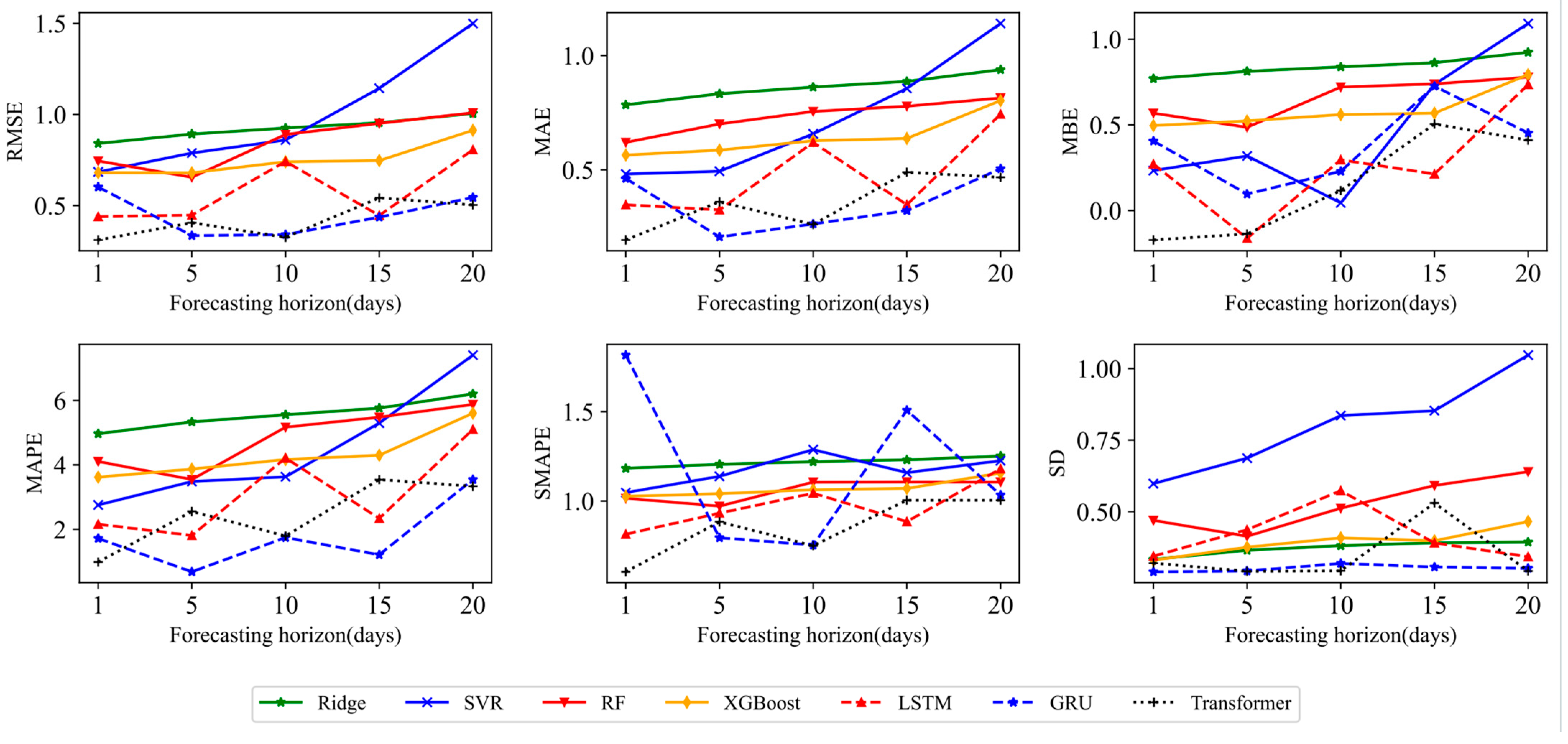
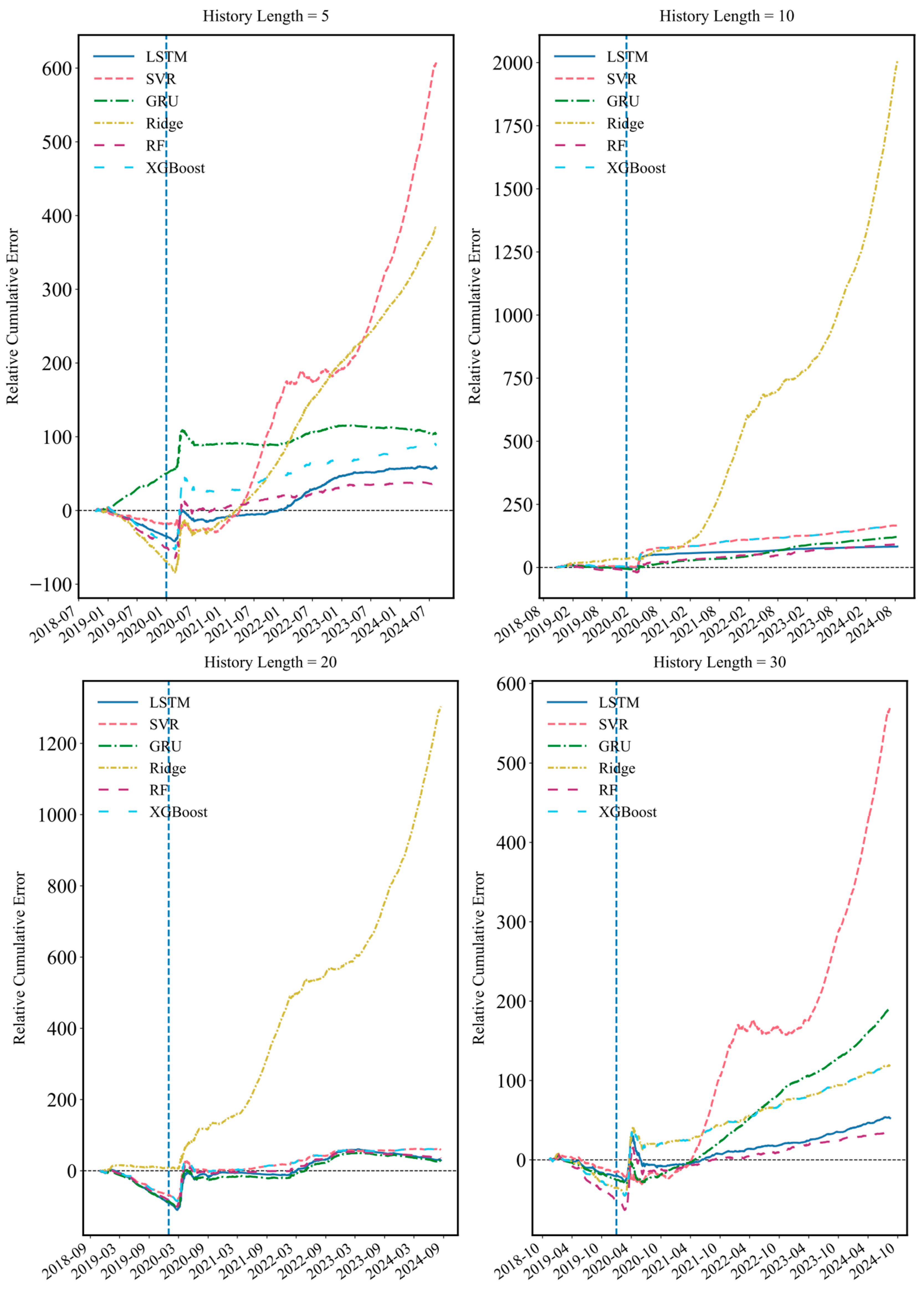
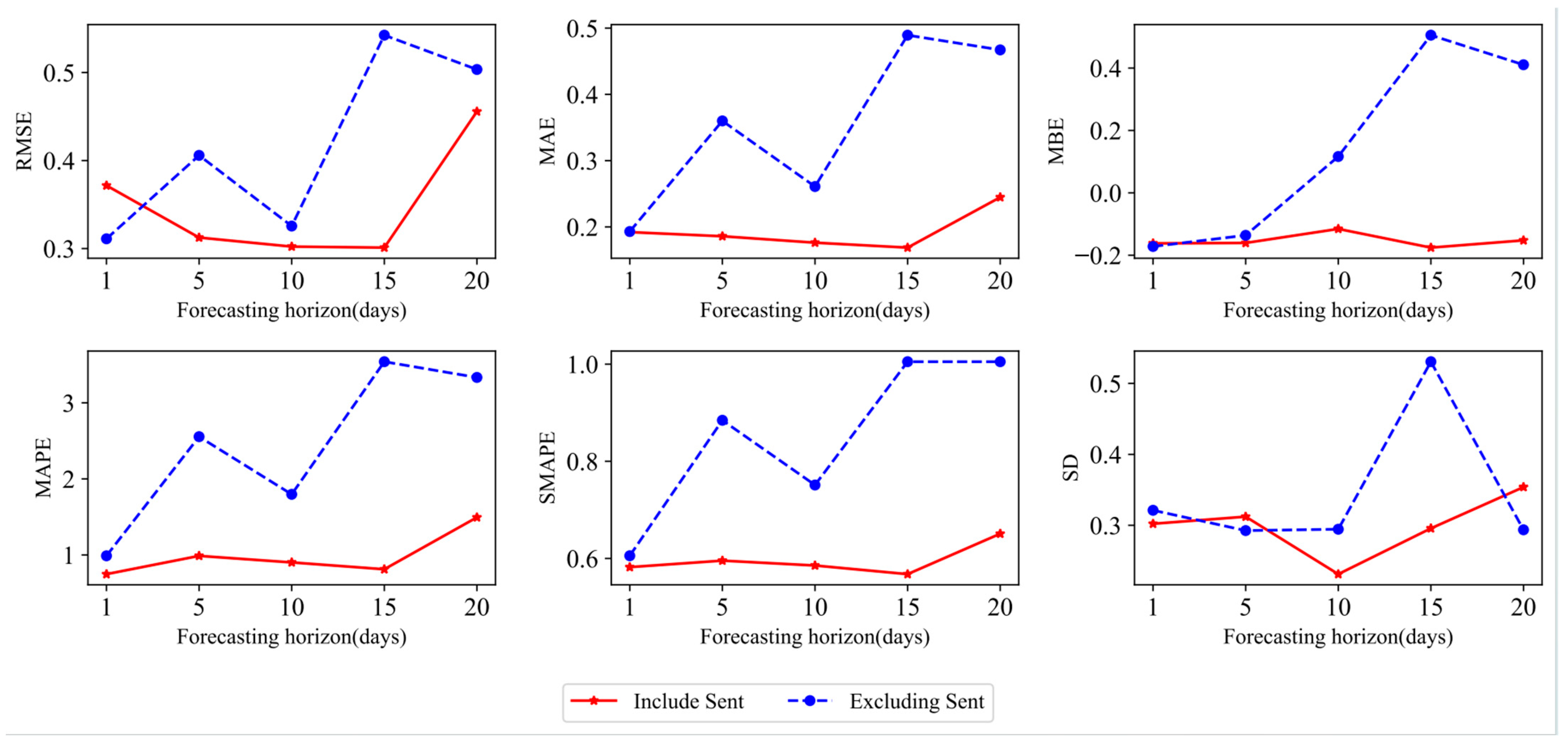
This paper mainly draws the following three conclusions. First, the degree of use of historical information will affect the prediction effect of various models. In this paper, the rolling window sizes of 5, 10, 20, and 30 are used for empirical analysis to verify the prediction advantage when the window size is set to 20, which provides strong data support for selecting the optimal historical data length. Second, the Transformer model has the best prediction accuracy in one-step prediction. RMSE, MAE, MAPE, SMAPE, MBE, and SD are used to evaluate the prediction effect of the seven models. Compared with each model, the average improvement ratios of the Transformer model under SSE are 0.5223, 0.2003, 0.6233, and 0.6033, 37.57%, and 18.70%, respectively. In particular, the Transformer model is compared with the traditional deep learning model, and the improvement ratio of each evaluation criterion is more than 30%. The Transformer model can maintain a certain degree of accuracy in prediction due to its self-attention mechanism, location coding positioning, and parallel processing capabilities, which make the model efficient in capturing long-distance dependencies in time series prediction. Third, according to the prediction results of various models in the multi-step prediction scenario, it can be found that the Transformer model not only has advantages in prediction accuracy but also shows significant stability in long-term RDS prediction. The DM test is used to compare the advantages and disadvantages of the model, and it is found that all DM test statistics of the Transformer model are positive, which further confirms the superiority and stability of the Transformer model in long-term prediction, and the potential of grasping the long-term dependence relationship of nonlinear and non-stationary complex data. The robustness of the Transformer model and the advantages of the stacked hybrid model are further confirmed in the discussion of robustness under structural fracture, the influence of the emotion index on model prediction, and RDS prediction results under the stacked ML-DL framework.

The research in this paper provides empirical support for the deep learning prediction of RDS. In future volatility research, the architecture and parameters of the Transformer model can be further improved and optimized, such as introducing new attention mechanisms and adjusting the number of attention heads, learning rate, and batch size, to find a better model structure and configuration. In addition, this paper focuses on the model construction and prediction result analysis of the downside risk indicator RDS. In terms of investment decision-making and risk management, future studies may explore the economic impact of prediction models, such as using model prediction results to assist investors in formulating specific trading strategies and helping risk managers optimize investment strategies, to further enhance the application value of prediction models.

References

1. Yu, Y.; Lin, Y.; Hou, X.; Zhang, X. Novel optimization approach for realized volatility forecast of stock price index based on deep reinforcement learning model. Expert. Syst. Appl. 2023, 233, 120880. [Google Scholar] [CrossRef]
2. Engle, R.F. Autoregressive Conditional Heteroscedasticity with Estimates of the Variance of United Kingdom Inflation. Econometrica 1982, 50, 987–1007. [Google Scholar] [CrossRef]
3. Bollerslev, T. Generalized autoregressive conditional heteroskedasticity. J. Econom. 1986, 31, 307–327. [Google Scholar] [CrossRef]
4. Taylor, S.J. Modeling Stochastic Volatility: A Review and Comparative Study. Math. Financ. 1994, 4, 183–204. [Google Scholar] [CrossRef]
5. Andersen, T.G.; Bollerslev, T. Answering the skeptics: Yes, standard volatility models do provide accurate forecasts. Int. Econ. Rev. 1998, 39, 885–905. [Google Scholar] [CrossRef]
6. Andersen, T.G.; Bollerslev, T.; Diebold, F.X.; Labys, P. Modeling and forecasting realized volatility. Econometrica 2003, 71, 579–625. [Google Scholar] [CrossRef]
7. Corsi, F. A simple approximate long-memory model of realized volatility. J. Financ. Econom. 2009, 7, 174–196. [Google Scholar] [CrossRef]
8. Izzeldin, M.; Hassan, M.K.; Pappas, V.; Tsionas, M. Forecasting realised volatility using ARFIMA and HAR models. Quant. Financ. 2019, 19, 1627–1638. [Google Scholar] [CrossRef]
9. Liang, C.; Wei, Y.; Lei, L.; Ma, F. Global equity market volatility forecasting: New evidence. Int. J. Financ. Econ. 2022, 27, 594–609. [Google Scholar] [CrossRef]
10. Korkusuz, B.; Kambouroudis, D.; McMillan, D.G. Do extreme range estimators improve realized volatility forecasts? Evidence from G7 Stock Markets. Financ. Res. Lett. 2023, 55, 103992. [Google Scholar] [CrossRef]
11. Fałdziński, M.; Fiszeder, P.; Orzeszko, W. Forecasting volatility of energy commodities: Comparison of garch models with support vector regression. Energies 2021, 14, 6. [Google Scholar] [CrossRef]
12. Luong, C.; Dokuchaev, N. Forecasting of Realised Volatility with the Random Forests Algorithm. J. Risk Financ. Manag. 2018, 11, 61. [Google Scholar] [CrossRef]
13. Demirer, R.; Gkillas, K.; Gupta, R.; Pierdzioch, C. Risk aversion and the predictability of crude oil market volatility: A forecasting experiment with random forests. J. Oper. Res. Soc. 2022, 73, 1755–1767. [Google Scholar] [CrossRef]
14. Jia, F.; Yang, B. Forecasting volatility of stock index: Deep learning model with likelihood-based loss function. Complexity 2021, 2021, 1–13. [Google Scholar] [CrossRef]
15. Zhang, C.-X.; Li, J.; Huang, X.-F.; Zhang, J.-S.; Huang, H.-C. Forecasting stock volatility and value-at-risk based on temporal convolutional networks. Expert. Syst. Appl. 2022, 207, 117951. [Google Scholar] [CrossRef]
16. Koo, E.; Kim, G. A new neural network approach for predicting the volatility of stock market. Comput. Econ. 2023, 61, 1665–1679. [Google Scholar] [CrossRef]
17. Todorova, N.; Souček, M. Overnight information flow and realized volatility forecasting. Financ. Res. Lett. 2014, 11, 420–428. [Google Scholar] [CrossRef]
18. Audrino, F.; Sigrist, F.; Ballinari, D. The impact of sentiment and attention measures on stock market volatility. Int. J. Forecast. 2020, 36, 334–357. [Google Scholar] [CrossRef]
19. Kim, D.; Baek, C. Factor-augmented HAR model improves realized volatility forecasting. Appl. Econ. Lett. 2020, 27, 1002–1009. [Google Scholar] [CrossRef]
20. Kambouroudis, D.S.; McMillan, D.G.; Tsakou, K. Forecasting realized volatility: The role of implied volatility, leverage effect, overnight returns, and volatility of realized volatility. J. Futures Mark. 2021, 41, 1618–1639. [Google Scholar] [CrossRef]
21. Lei, B.; Liu, Z.; Song, Y. On stock volatility forecasting based on text mining and deep learning under high-frequency data. J. Forecast. 2021, 40, 1596–1610. [Google Scholar] [CrossRef]
22. Jiao, X.R.; Song, Y.P.; Kong, Y.; Tang, X.L. Volatility forecasting for crude oil based on text information and deep learning PSO-LSTM model. J. Forecast. 2022, 41, 933–944. [Google Scholar]
23. Ma, W.; Hong, Y.; Song, Y. On stock volatility forecasting under mixed-frequency data based on hybrid RR-MIDAS and CNN-LSTM models. Mathematics 2024, 12, 1538. [Google Scholar] [CrossRef]
24. Zhang, Y.; Song, Y.; Peng, Y.; Wang, H. Volatility forecasting incorporating intraday positive and negative jumps based on deep learning model. J. Forecast. 2024, 43, 2749–2765. [Google Scholar]
25. Granger, C.W.J. In Praise of Pragmatic Econometrics. In The Methodology and Practice of Econometrics: A Festschrift in Honour of David F. Hendry, 1st ed.; Castle, J.L., Shephard, N., Eds.; Oxford University Press: Oxford, UK, 2008; pp. 105–116. [Google Scholar]
26. Barndorff-Nielsen, O.; Kinnebrock, S.; Shephard, N. Measuring downside risk-realised semivariance. In Volatility and Time Series Econometrics: Essays in Honor of Robert Engle, 1st ed.; Bollerslev, T., Jeffrey, R., Mark, W., Eds.; Oxford Academic: Oxford, UK, 2010; Volume 7, pp. 117–136. [Google Scholar]
27. Vaswani, A.; Shazeer, N.; Parmar, N.; Uszkoreit, J.; Jones, L.; Gomez, A.N.; Kaiser, Ł.; Polosukhin, I. Attention Is All You Need. arXiv 2017, arXiv:1706.03762. [Google Scholar]
28. Asgarkhani, N.; Kazemi, F.; Jakubczyk-Gałczyńska, A.; Mohebi, B.; Jankowski, R. Seismic response and performance prediction of steel buckling-restrained braced frames using machine-learning methods. Eng. App. Artif. Intell. 2024, 128, 107388. [Google Scholar] [CrossRef]
29. Kazemi, F.; Asgarkhani, N.; Jankowski, R. Optimization-based stacked machine-learning method for seismic probability and risk assessment of reinforced concrete shear walls. Expert. Syst. Appl. 2024, 255, 124897. [Google Scholar]
30. Diebold, F.X.; Mariano, R.S. Comparing predictive accuracy. J. Bus. Econ. Stat. 2022, 20, 134–144. [Google Scholar]
31. Devlin, J.; Chang, M.W.; Lee, K.; Toutanova, K. Bert: Pre-training of deep bidirectional transformers for language understanding. arXiv 2018, arXiv:1810.04805. [Google Scholar]
32. Antweiler, W.; Frank, M.Z. Is all that talk just noise? The information content of internet stock message boards. J. Financ. 2004, 59, 1259–1294. [Google Scholar] [CrossRef]
Figure 1. Transformer structure.
Mathematics 13 01260 g001
Figure 2. RDS chart of the SSE stock index.
Mathematics 13 01260 g002
Figure 3. Spearman correlation coefficient heatmap of predictor and predicted variables of SSE.
Mathematics 13 01260 g003
Figure 4. Schematic diagram of rolling prediction.
Mathematics 13 01260 g004
Figure 5. Under SSE, the change trend chart of each evaluation criteria is predicted using different models under different forecasting history lengths.
Mathematics 13 01260 g005
Figure 6. Under SSE, the change trend chart of each evaluation criteria based on different prediction models and various forecasting horizons is shown.
Mathematics 13 01260 g006
Figure 7. Cumulative relative errors of the Transformer model versus other models at various historical lengths under SSE.
Mathematics 13 01260 g007
Figure 8. Dual coordinate main view of RDS and the sentiment indicator under SSE.
Mathematics 13 01260 g008
Figure 9. Evaluation criteria change trend chart of the Transformer model with or without the sentiment factor under different history lengths of SSE.
Mathematics 13 01260 g009
Figure 10. Change trend chart of each evaluation criteria of the Transformer model with or without the emotion factor under different forecasting horizons of SSE.
Mathematics 13 01260 g010