Article

Control of Vehicle Lateral Handling Stability Considering Time-Varying Full-State Constraints

School of Mechanical Engineering, Yanshan University, Qinhuangdao 066004, China
*
Author to whom correspondence should be addressed.
Mathematics 2025, 13(8), 1217; https://doi.org/10.3390/math13081217
Submission received: 13 February 2025 / Revised: 21 March 2025 / Accepted: 1 April 2025 / Published: 8 April 2025

Abstract

:
Lateral handling stability control is crucial for ensuring vehicle driving safety. To address this issue, this paper proposes a lateral handling stability control method that considers time-varying full-state constraints. By constructing a time-varying symmetric Barrier Lyapunov Function (TS-BLF), this method imposes time-varying nonlinear constraints on both the sideslip angle and yaw rate, thereby ensuring full-state constrained stability control of vehicles under complex operating conditions. Additionally, a second-order command filtering technique with an error compensation mechanism is introduced to reduce the computational complexity of control laws while mitigating filter-induced errors that may degrade system performance. To validate the effectiveness and robustness of the proposed method, the vehicle’s dynamic response is analyzed under different speeds on both dry asphalt pavement and dry gravel surfaces. The simulation results demonstrate that the proposed method effectively suppresses understeer and oversteer, enhances the dynamic stability margin under extreme operating conditions, and improves vehicle adaptability in complex environments.

1. Introduction

With the rapid development of intelligent vehicle technology, lateral handling stability control has become a key factor in enhancing the active safety of the entire vehicle. Its control performance is directly related to the driving safety margin under complex operating conditions. In dynamic and intricate traffic scenarios, vehicles are prone to trajectory tracking deviations during steering maneuvers. Such deviations not only induce lateral instability phenomena such as understeer or oversteer but also cause the nonlinear distortion of vehicle lateral dynamics characteristics. These unstable conditions significantly degrade path-following accuracy, exacerbate tire force saturation phenomena, and trigger chain reactions of yaw moment imbalance, ultimately leading to the drastic deterioration of control system robustness. Particularly under critical conditions, such dynamic instabilities may induce severe accidents like vehicle sideslips or rollovers.
Therefore, enhancing vehicle lateral handling stability based on active safety control technology [1] has become one of the core issues in the field of intelligent vehicle safety research. Direct yaw-moment control (DYC) [2], as a core technology in the field of vehicle lateral active safety control, operates based on the principle of actively adjusting the longitudinal force distribution among the wheels to generate a compensatory yaw moment, thereby achieving precise tracking of the vehicle’s intended trajectory. Based on a multi-actuator-coordinated control framework, this technology establishes an asymmetric longitudinal force distribution mechanism by applying differentiated driving or braking torques to different wheels, thereby generating controllable yaw moments around the vehicle’s center of mass. During near-critical stability conditions, particularly in extreme scenarios such as emergency steering or low-adhesion road surfaces, DYC effectively compensates for any understeer/oversteer caused by tire nonlinear characteristics while suppressing lateral velocity divergence through moment compensation mechanisms, thereby significantly improving vehicle lateral stability.
Direct yaw control (DYC) has emerged as a key research focus in vehicle active safety control, leading to the development of various control strategies, including robust control [3,4,5], sliding mode variable structure control [6,7,8], fuzzy control [9,10,11], and model predictive control (MPC) [12,13,14], among others. Although these control strategies have demonstrated certain effectiveness in practical applications, most methods have yet to systematically address the constraints on key state variables, such as vehicle sideslip angle and yaw rate, from a theoretical perspective. MPC, as an optimization-based control approach, is particularly well suited for handling state constraints and can dynamically adjust control inputs in real time through a receding horizon optimization strategy. However, this method requires the resolution of an optimization problem online at each control cycle to determine the optimal control input. As system complexity increases, the size of the optimization problem and the associated computational burden grow accordingly, potentially leading to excessive computation time, which may hinder the real-time performance required for vehicle dynamic stability control.
In contrast, control methodologies based on the Barrier Lyapunov Function (BLF) [15] explicitly incorporate both time-varying and time-invariant state constraints during controller design. This approach not only ensures system stability but also enhances the flexibility and robustness of control strategies. Such BLF-based methods have exhibited strong adaptability and engineering applicability across multiple industrial control domains. For example, in the field of quadrotor UAV control, Reference [16] proposed a novel adaptive finite-time controller for a state-constrained quadrotor UAV subject to stochastic perturbations and unknown parameters. This method integrated full-state quantization and Barrier Lyapunov Functions to ensure constraint satisfaction and adaptive performance, with stability formally proven via Lyapunov theory and effectiveness validated through experimental simulations. Reference [17] presented a fault-tolerant trajectory tracking controller for state-constrained quadrotors, incorporating an adaptive Nussbaum-type function-based control scheme combined with a nonlinear mapping technique. This approach mitigated numerical instability and addressed input saturation, ensuring robust performance under time-varying actuator faults. Stability was rigorously established through Lyapunov analysis, and the numerical simulations confirmed the method’s effectiveness. Reference [18] introduced an event-triggered finite-time adaptive fuzzy control strategy for quadrotor UAVs with asymmetric time-varying state constraints and unknown disturbances. This strategy integrated a fuzzy logic system for nonlinear approximation, a disturbance observer for compensation, and a command filter to reduce computational complexity and communication burden. The proposed method guarantees finite-time stability while ensuring all state constraints are satisfied, with effectiveness validated through simulations. In the field of robotic manipulator control, Reference [19] presented an adaptive neural network-based fault-tolerant control scheme for a flexible manipulator system with uncertain dynamics and state constraints. This approach employed tangent Barrier Lyapunov Functions to enforce constraint satisfaction, neural networks to approximate system uncertainties, and a backstepping framework to design controllers that ensure bounded closed-loop signals. System stability was rigorously verified through Lyapunov analysis, and the effectiveness of the method proposed was demonstrated via simulations. Reference [20] focused on adaptive neural tracking control for a flexible manipulator system with time-varying full-state constraints. This method leveraged neural networks to approximate unknown nonlinearities, utilized backstepping to design an adaptive boundary controller that mitigates input saturation, and incorporated an asymmetric time-varying Barrier Lyapunov Function to guarantee state constraint enforcement and bounded closed-loop signals. The effectiveness of the approach was validated through simulations. In the field of motor control, Reference [21] presented a state-saturated second-order sliding mode (SOSM) controller for permanent magnet synchronous motor (PMSM) systems, designed to enhance robustness, enforce state constraints, and mitigate excessive transient currents. The stability of the proposed controller was rigorously proven via Lyapunov theory, and its effectiveness was validated through both simulations and experiments. The results demonstrated superior performance over traditional control strategies in terms of robustness and transient current management. Reference [22] proposed an adaptive fuzzy finite-time command filtered control (FTCFC) strategy for stochastic PMSM systems. This approach integrated Barrier Lyapunov Functions, fuzzy logic systems, and command-filtered backstepping to ensure state constraint satisfaction, finite-time tracking performance, and signal boundedness. Simulation results confirmed the effectiveness of the proposed strategy. Reference [23] introduced a composite Barrier Function-based Sliding Mode Control (BFSMC) approach for PMSM systems to address speed fluctuation constraints (SFC) under multiple disturbances. The method incorporated a disturbance observer to handle lumped disturbances and employed a flexible switching gain to reduce chattering. Stability was formally analyzed, and the effectiveness of the approach was validated through both simulations and experiments. Reference [24] proposed a safety-critical generalized predictive control (SCGPC) approach for PMSM systems. This method integrated Control Barrier Functions (CBF) to explicitly consider current and voltage constraints and introduced a disturbance observer-based, dynamic, robust CBF to ensure current safety. Simulations and experimental results demonstrate its effectiveness and superiority over existing methods.
Although state-constrained control techniques based on BLF have demonstrated significant advantages in both time-varying and non-time-varying systems, the controller design process involves the recursive differentiation of virtual control laws across multiple layers. This leads to an exponential increase in differentiation complexity, causing the so-called “computational burden” problem, which severely limits the practical feasibility of this approach in real-time engineering applications. To overcome this bottleneck, Command-Filtered Control (CFC) [25] introduces a dynamic error compensation mechanism, which actively suppresses the accumulation of filtering errors and effectively mitigates the error propagation and amplification issues commonly observed in conventional backstepping methods. Additionally, CFC employs a multi-order command filtering strategy to perform a frequency-domain shaping of the control signals, thereby preserving the system’s original dynamic characteristics while significantly reducing the coupling interference between actuator high-frequency chattering and sensor noise. This approach not only alleviates computational burden but also enhances the overall closed-loop system performance in terms of both frequency response and robust stability. For example, Reference [26] presented an adaptive neural tracking control strategy for nonlinear MIMO state-constrained systems with input delay and saturation. This approach leveraged neural networks for nonlinear approximation, Barrier Lyapunov Functions to enforce state constraints, and command-filtered backstepping to handle input saturation and reduce computational complexity. Simulation results confirm the effectiveness of the proposed method. Reference [27] developed a command filter-based finite-time tracking control strategy for fractional-order nonlinear constrained systems with saturated inputs. The method introduced a novel Lyapunov stability lemma, an enhanced error compensation system, and auxiliary signals to ensure finite-time convergence, effectively handle state constraints, and eliminate the need for feasibility conditions. The simulations demonstrated the system’s effectiveness in achieving robust tracking performance. Reference [28] proposed a robust command-filtered control method with prescribed performance for flexible-joint robots, addressing both matched and mismatched disturbances through generalized proportional–integral observers. The approach incorporated a global prescribed performance function, employed a second-order command filter, and integrated an error compensation system to prevent computational complexity explosion. The theoretical analysis and experimental results validate the method’s efficacy.
Based on the above analysis, our previous research investigated a vehicle yaw stability control method considering time-invariant full-state constraints [29]. The effectiveness of this method was validated through stability proof and simulation analysis. However, this approach had certain limitations, as it is only valid under ideal conditions, which restricted its feasibility for engineering applications. To address this issue, building upon our previous work, this paper proposes a vehicle lateral handling stability control method based on time-varying full-state constraints for vehicles equipped with conventional hydraulic braking systems. This method expands the applicable range by incorporating time-varying dynamic constraints and the tracking of the vehicle’s sideslip angle while ensuring that the yaw rate always satisfies predefined constraint conditions. Theoretically, it provides a feasible solution for vehicle lateral handling stability control. Simulation experiments further validate the effectiveness of the proposed control algorithm, with its main advantages including the following:
1.
Adaptability to dynamically changing state constraints for enhanced vehicle safety.
Conventional state constraint control methods based on non-time-varying Barrier Lyapunov Functions typically employ fixed constraints. In contrast, the proposed method introduces time-varying full-state constraints, enabling a dynamic adjustment of the constraint limits for the vehicle’s sideslip angle and yaw rate based on real-time driving conditions, such as speed and tire–road adhesion coefficient. This adaptive approach enhances the flexibility and robustness of the control strategy, ensuring that the vehicle operates within a safe and stable region as much as possible, thereby reducing the risk of loss of control.
2.
Simultaneous consideration of constraint satisfaction and control performance for enhanced adaptability under complex driving conditions.
The integration of time-varying full-state constraints with command filtering enables the control strategy to dynamically adjust control inputs under challenging driving scenarios, such as high-speed lane changes, emergency obstacle avoidance, and low-adhesion road surfaces. This ensures that state constraints are satisfied without overly conservative restrictions on vehicle dynamics, thereby achieving an optimal balance between stability and maneuverability.

2. Vehicle Lateral Handling Stability Control Process

Figure 1 illustrates the hierarchical control process for vehicle lateral handling stability. First, the upper-layer lateral handling stability command filtering controller, based on time-varying full-state constraints, compensates in real time for the deviation between the desired and actual vehicle sideslip angles to generate an additional yaw moment. Subsequently, this corrected yaw moment is precisely applied to specific wheels through the lower-layer unilateral wheel braking torque distribution strategy to achieve accurate yaw motion control. It is worth noting that the coupled dynamic model [30], the vertical load dynamic distribution algorithm, the Dugoff tire model [31], and the additional yaw moment distribution based on unilateral wheel braking [32,33], as discussed in this paper, have been thoroughly analyzed in our previous research [29] and will not be elaborated here. Instead, this study focuses on the design of the novel control strategy, stability analysis, and the validation of control effectiveness.

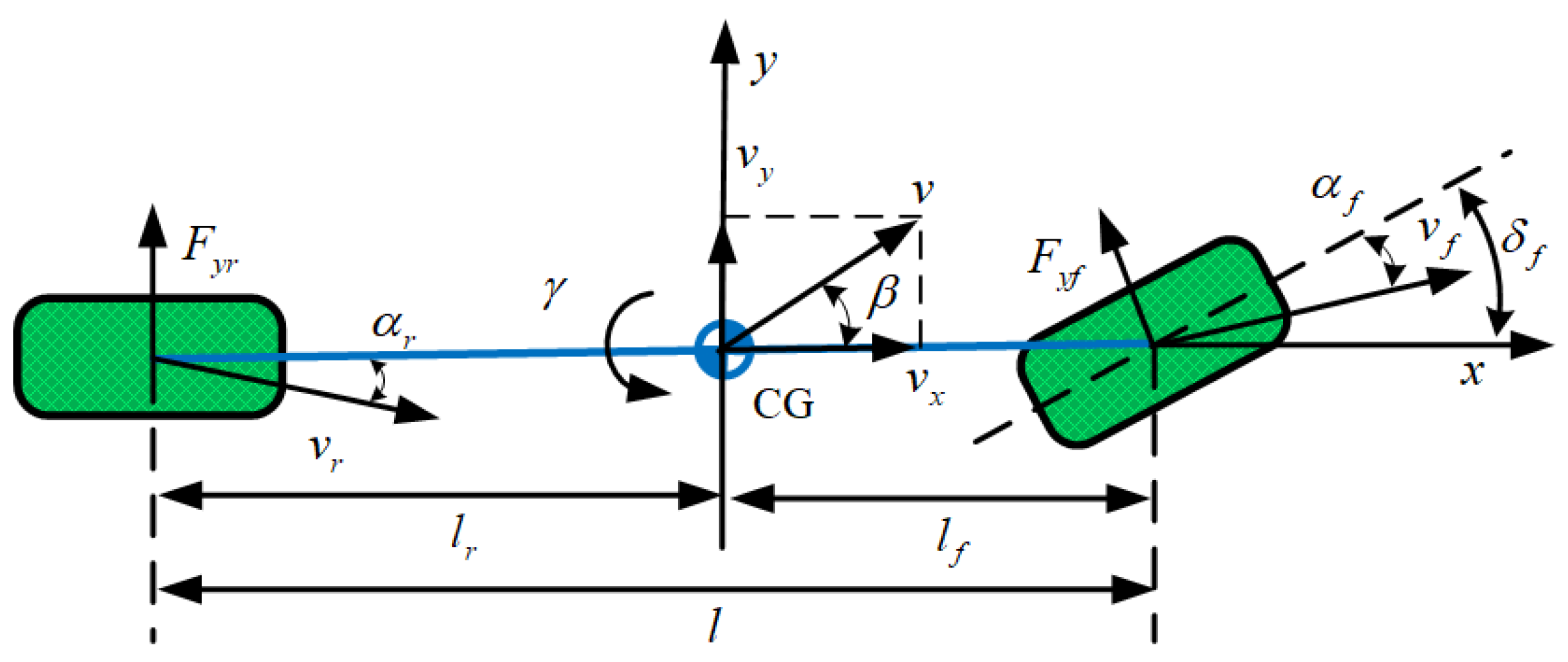
3. Simplification and Problem Formulation of the Coupled Vehicle Dynamics Model

Simplification of the Coupled Vehicle Dynamics Model

The linear two-degree-of-freedom (2-DOF) vehicle model features a relatively simple mathematical representation while incorporating the key state variables required for direct yaw moment control, namely yaw rate and vehicle sideslip angle. Considering the simplicity of controller design, this study appropriately simplifies the vehicle dynamics model and adopts the linear 2-DOF model [34] as the foundation for controller development, as illustrated in Figure 2. An additional yaw moment is introduced into this model to enable effective yaw stability control.
m v ˙ y + γ v x = F y f cos δ f + F y r I z γ ˙ = l f F y f cos δ f l r F y r + Δ M
α f = δ f + β + l f γ v x α r = β l r γ v x
where F y f = k f α f , F y r = k r α r , with k f and k r represent the cornering stiffness of the front and rear axles, respectively.
Assuming a small front-wheel steering angle, we have cos δ f 1 and β v y / v x . Thus, the linearized two-degree-of-freedom model is given by the following:
β ˙ = k f + k r m v x β k f m v x δ f + l f k f l r k r m v x 2 1 γ γ ˙ = l f k f l r k r I z β + l f k f 2 l r k r 2 I z v x γ l f k f I z δ f + 1 I z Δ M
Defining the state variables as the vehicle’s centroid sideslip angle x 1 = β and yaw rate x 2 = γ , the state Equations can be expressed as follows:
x ˙ 1 = f 1 x 1 + g 1 x 2 x ˙ 2 = f 2 x 1 ,   x 2 + d u y = x 1
where
f 1 x 1 = k f + k r m v x x 1 k f m v x δ f ,   g 1 = l f k f l r k r m v x 2 1 , f 2 x 1 ,   x 2 = l f k f l r k r I z x 1 + l f k f 2 l r k r 2 I z v x x 2 l f k f I z δ f ,   d = 1 I z ,   u = Δ M .
The control objective of this study is to design a control law u = Δ M to ensure that the vehicle’s centroid sideslip angle x 1 tracks the desired value y d , while keeping the error variables v i i = 1 , 2 and state variables x i i = 1 , 2 constrained within the compact sets Ω v = v i < k b i t , i = 1 , 2 and Ω x = x i < k c i t , i = 1 , 2 , respectively.
Assumption 1.
Let y d t be the desired tracking signal, where both y d t and its first derivative y ˙ d t are known, smooth, and bounded. There exist positive constants Y 0 and Y 1 such that y d t Y 0 < k c 1 , y ˙ d t Y 1 , t 0 .
Lemma 1.
From Equation (5), it can be observed that the second-order command filtering structure is shown in Figure 3. The corresponding state Equations are as follows:
z ˙ i , 1 z ˙ i , 2 = 0 1 ω n i 2 2 ζ i ω n i z i , 1 z i , 2 + 0 ω n i 2 φ i
where κ i = z i , 1  and κ ˙ i = ω n z i , 2  represent the two outputs of the command filter; φ i  is the input to the command filter; the initial states of the command filter are φ i 0 = z i , 1 0  and z i , 2 0 = 0 ; ζ i  is the damping of the filter, with ζ i 0 , 1 ; and ω n i  is the bandwidth of the filter. According to Reference [25], when  φ i  is bound and φ ˙ i  and φ ¨ i  are both bound and continuous, for any given η > 0 , there exist ζ i  and ω n i  such that the filtering error κ i φ i η  and κ ˙ i φ ˙ i η . Theoretically, by appropriately tuning the damping ζ i  and bandwidth ω n i , the tracking accuracy can be significantly improved.
Lemma 2
([35]). For any vectors σ i n and v i n , if v i < σ i , then the following inequality holds:
log σ i 2 σ i 2 v i 2 σ i 2 σ i 2 v i 2
Lemma 3
([15]). For any positive integers k b i , i = 1 ,   ,   n , let Γ : = R l × R n R l + n and B 1 : = υ R : v i t < k b i , i = 1 , , n , t 0 R n be open sets. Consider the system ξ ˙ = f ξ , u , where ξ : = ϕ , v i T Γ and ϕ are free state variables, v i is a constrained state variable, and f : = R + × Γ R l + n is piecewise continuous. When ξ satisfies the local Lipschitz condition, assume that there exist functions U : R l R + and V 1 : B 1 R + that are continuously differentiable and positive definite in their respective domains. Then, the following conditions hold:
 
When v i k b i , V i v i .
 
γ 1 ϕ U ϕ γ 2 ϕ .
Here, γ 1 and γ 2 are of class k functions. Let V ξ : = V i v i + U ϕ . If the following inequality in Equation (7) holds:
V ˙ = V ξ f a 0 V v + b 0
and a 0 > 0 , b 0 > 0 , then for any t 0 , , v i t B 1 .
Remark 1.
For the problem studied in this paper, a logarithmic Barrier Lyapunov Function V x = log a 2 a 2 x 2 is chosen, as shown in Figure 4. For this system, the logarithmic Barrier Lyapunov Function V x is a scalar function that is continuous and positive definite on . The boundaries of V x along the x-axis are −a and a, where a is a positive constant. As x approaches −a or a, V x [36].

4. Design and Stability Analysis of Vehicle Lateral Handling Stability Controller with Time-Varying Full-State Constraints

4.1. Controller Design

Define the error variable as follows:
e 1 = x 1 y d ,   e 2 = x 2 κ 1
where κ 1 represents the output signal of the command filter.
The compensated tracking error subsystem is selected as follows:
v 1 = e 1 δ 1 ,   v 2 = e 2 δ 2
Taking the derivative of Equation (9) gives the following:
v ˙ 1 = x ˙ 1 y ˙ d δ ˙ 1
Step 1. For the first error subsystem v 1 , select TS-BLF.
V 1 v 1 = 1 2 log k b 1 2 k b 1 2 v 1 2
Taking the derivative of Equation (11) gives the following:
V ˙ 1 v 1 = v 1 k b 1 2 v 1 2 v ˙ 1 k ˙ b 1 k b 1 v 1 = v 1 k b 1 2 v 1 2 v ˙ 1 δ ˙ 1 k ˙ b 1 k b 1 v 1 = v 1 k b 1 2 v 1 2 x ˙ 1 y ˙ d + k 1 δ 1 g 1 κ 1 α 1 g 1 δ 2 k ˙ b 1 k b 1 v 1
Select the virtual control law as follows:
α 1 = 1 g 1 k 1 e 1 f 1 x 1 + y ˙ 1 d K ¯ 1 v 1
Among them, the time-varying constraint gain K ¯ 1 = k ˙ b 1 / k b 1 2 + ϑ .
Select the error compensation signal as follows:
δ ˙ 1 = k 1 δ 1 + g 1 κ 1 α 1 + g 1 δ 2
Note 1. It is worth noting that ϑ is a normal number and ensures that when k ˙ b 1 = 0 , K ¯ 1 = k ˙ b 1 / k b 1 2 + ϑ > 0 and thus K ¯ 1 + k ˙ b 1 / k b 1 > 0 .
Substituting Equations (13) and (14) into Equation (12) yields the following:
V ˙ 1 v 1 = k 1 v 1 k b 1 2 v 1 2 v 1 + g 1 v 1 k b 1 2 v 1 2 v 2 v 1 2 k b 1 2 v 1 2 K ¯ 1 + k ˙ b 1 k b 1 k 1 v 1 k b 1 2 v 1 2 v 1 + g 1 v 1 k b 1 2 v 1 2 v 2
Step 2. For the second error subsystem v 2 , select TS-BLF.
V 2 v 1 , v 2 = V 1 v 1 + 1 2 log k b 2 2 k b 2 2 v 2 2
Taking the derivative of Equation (16) yields the following:
V ˙ 2 v 1 , v 2 = k 1 v 1 k b 1 2 v 1 2 + g 1 v 1 k b 1 2 v 1 2 v 2 k ˙ b 2 v 2 2 k b 2 k b 2 2 v 2 2 + v 2 v ˙ 2 k b 2 2 v 2 2 = k 1 v 1 k b 1 2 v 1 2 + g 1 v 1 k b 1 2 v 1 2 v 2 k ˙ b 2 v 2 2 k b 2 k b 2 2 v 2 2 + v 2 f 2 x 1 , x 2 + d u κ ˙ 1 k b 2 2 v 2 2
Select the final control law as follows:
u = 1 d κ ˙ 1 f 2 x 1 , x 2 k 2 v 2 + k ˙ b 2 v 2 k b 2 K ¯ 2 v 2 g 1 v 1 k b 2 2 v 2 2 k b 1 2 v 1 2
Among them, the time-varying constraint gain K ¯ 2 = k ˙ b 2 / k b 2 2 + ϑ .
Substituting Equation (18) into Equation (17) yields the following:
V ˙ 2 v 1 , v 2 k 1 v 1 k b 1 2 v 1 2 k 2 v 2 2 k b 2 2 v 2 2
Note 2. Similarly, when k ˙ b 2 = 0 , it satisfies K ¯ 2 = k ˙ b 2 / k b 2 2 + ϑ > 0 .

4.2. Stability Analysis

Define the initial condition of the system as v i 0 < k b i 0 , and select the TS-BLF for the entire system as follows:
V = 1 2 log k b 1 2 k b 1 2 v 1 2 + 1 2 log k b 2 2 k b 2 2 v 2 2
Differentiating Equation (20) gives the following:
V ˙ k 1 v 1 k b 1 2 v 1 2 k 2 v 2 2 k b 2 2 v 2 2
From Equation (21) and Lemma 2, we can obtain the following:
V ˙ k 1 log k b 1 2 k b 1 2 v 1 2 + k 2 log k b 2 2 k b 2 2 v 2 2
Combining Equation (20), we get the following.
V ˙ ε V
In Equation (23), ε = 2 min k 1 ,     k 2 .
From Equation (23) and Reference [37], the following can be obtained:
d V t d t ε V t ,     t > 0
Multiply both sides of Equation (24) by e ε t and then integrate over 0 , t to obtain the following:
V t V 0 e ε t V 0 ,   for   t > 0 .
Further obtain the following:
lim t v i k b i 1 e 2 V 0 e ε t
Since e i = v i + δ i , and according to reference [38], δ i is bound. Assuming δ 1 χ , where χ is a normal number, then e 1 k b 1 1 e 2 V 0 e ε t + χ . Since v 1 = e 1 δ 1 and v 1 < k b 1 , then e 1 v 1 + δ 1 < k b 1 + δ 1 . From e 1 = x 1 y d , y d Y 0 , x 1 k b 1 + δ 1 + Y 0 = k c 1 . Because κ 1 is a function of e 1 and y ˙ d , κ 1 is bound. Let κ 1 satisfy κ 1 κ ¯ 1 , where κ ¯ 1 is a constant. Also, since v 2 = e 2 δ 2 and v 2 k b 2 , we can obtain e 2 v 2 + δ 2 < k b 2 + δ 2 , and from e 2 = x 2 κ 1 we can obtain x 2 k b 2 + δ 2 + κ ¯ 1 = k c 2 . In summary, all the state variables x i in the system are constrained within the compact set Ω x = x i < k c i t , i = 1 , 2 .

5. Simulation Verification and Result Analysis

5.1. Parameter Settings

To verify the effectiveness of the proposed lateral handling stability command filtering control method based on time-varying full-state constraints, the dynamic response characteristics of the proposed method and the uncontrolled vehicle are compared under the same double-lane-change front steering angle δ f conditions. The comparison is conducted on dry asphalt with a coefficient of friction of μ = 0.85 and dry gravel with a coefficient of friction of μ = 0.5 . The parameter settings of the vehicle model are as follows: m = 1412   kg ; I z = 1536.7   kg m 2 ; J = 0.9   kg m 2 ; R = 0.325   m ; b f = b r = 1.675   m ; h c g = 0.54   m ; g = 9.8   m / s 2 ; l f = 1.015   m ; l r = 1.895   m .
To ensure vehicle controllability and driving safety, the longitudinal velocity direction of the vehicle should be as aligned as possible with the driver’s facing direction. Therefore, in this study, the desired vehicle centroid sideslip angle β d is set to 0 rad [39]. However, as the centroid sideslip angle increases further, the driver’s control ability may deteriorate, potentially compromising driving safety. To address this, an empirical formula is employed to constrain the centroid sideslip angle within the range of β d tan 1 0.02   μ g [40]. Additionally, the yaw rate is constrained by the vehicle’s driving speed and road adhesion conditions. When the time-varying constraint γ 0.85 μ g / ν x [41] is satisfied, vehicle stability is maintained throughout the entire operating range, preventing the loss of control.

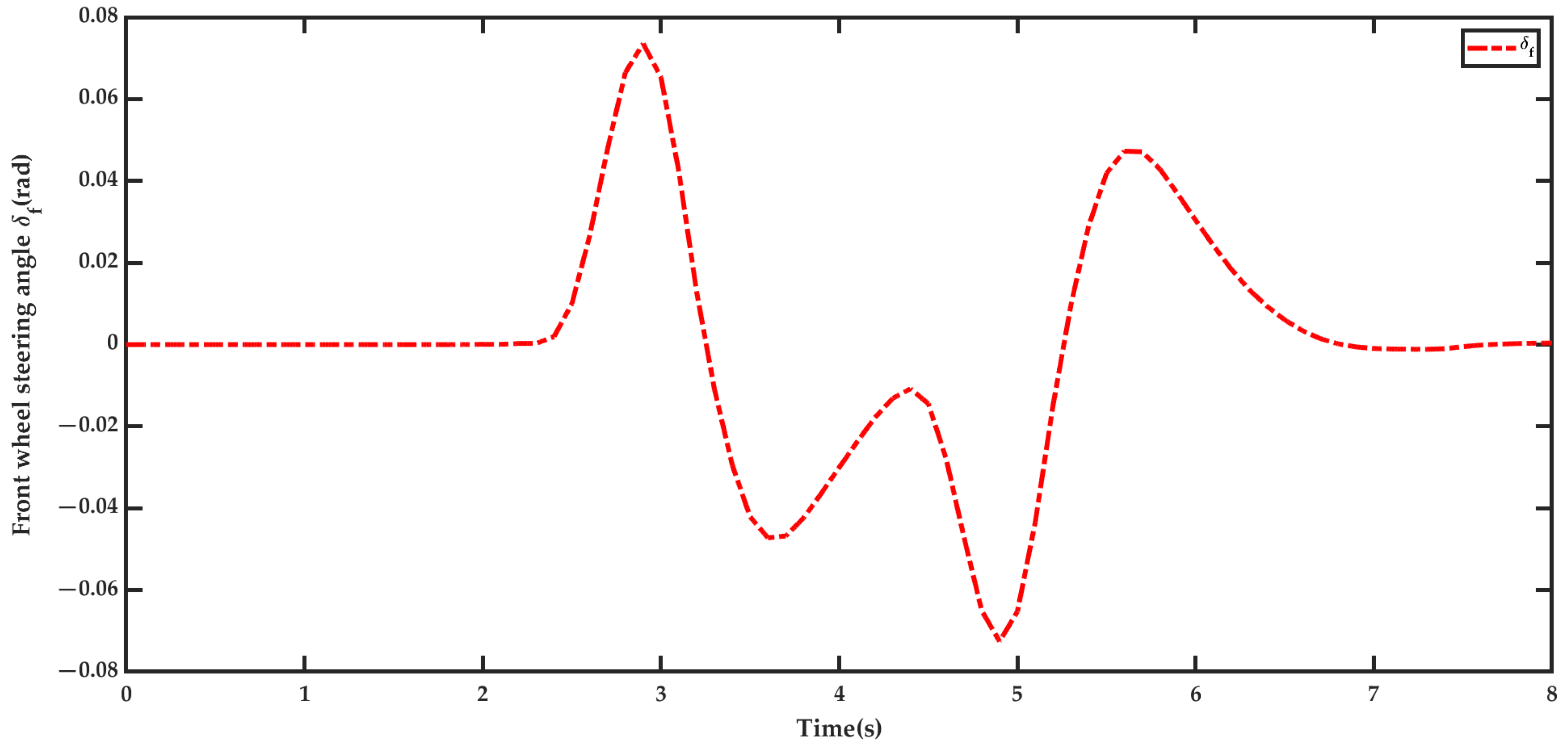
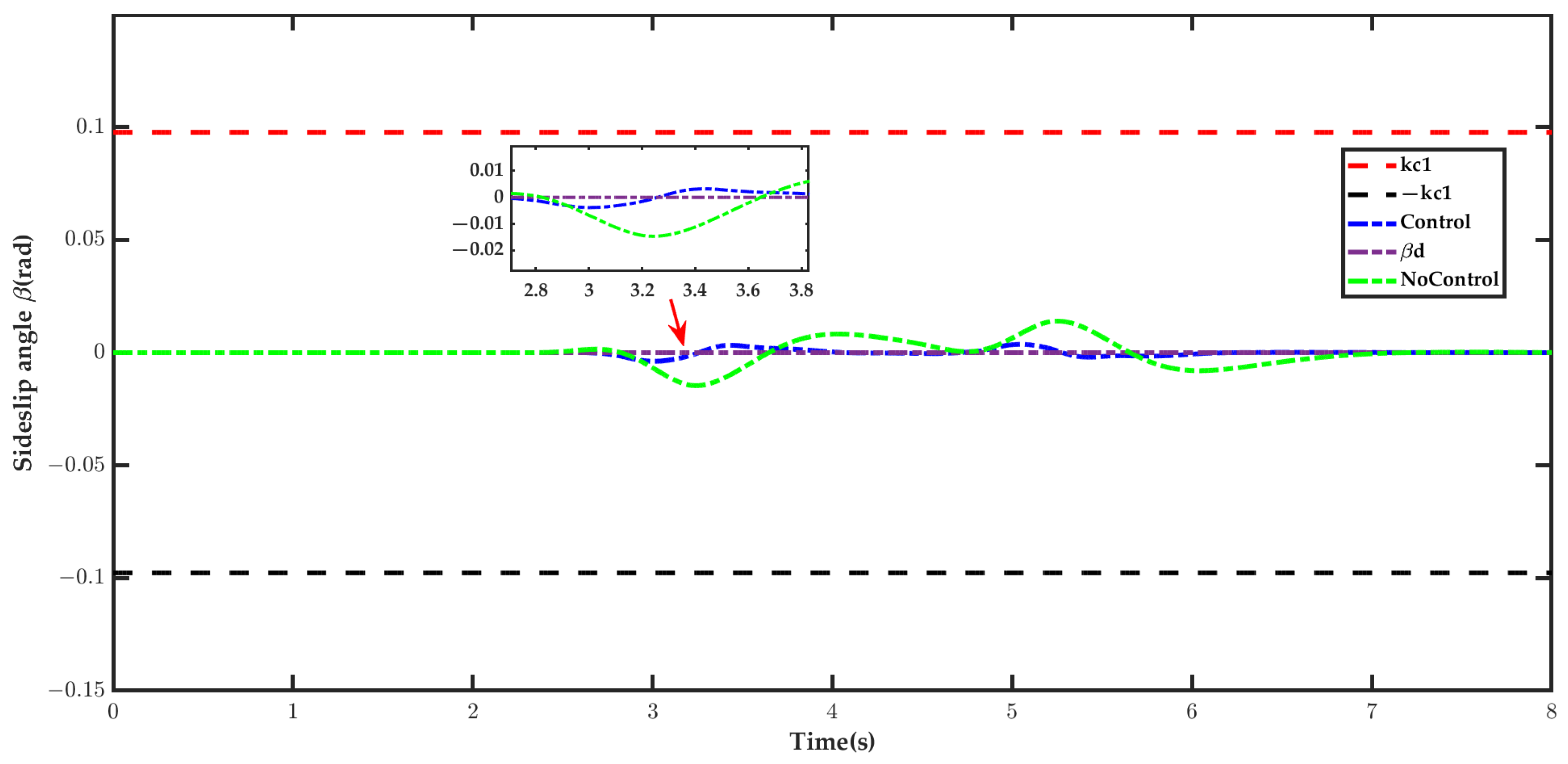
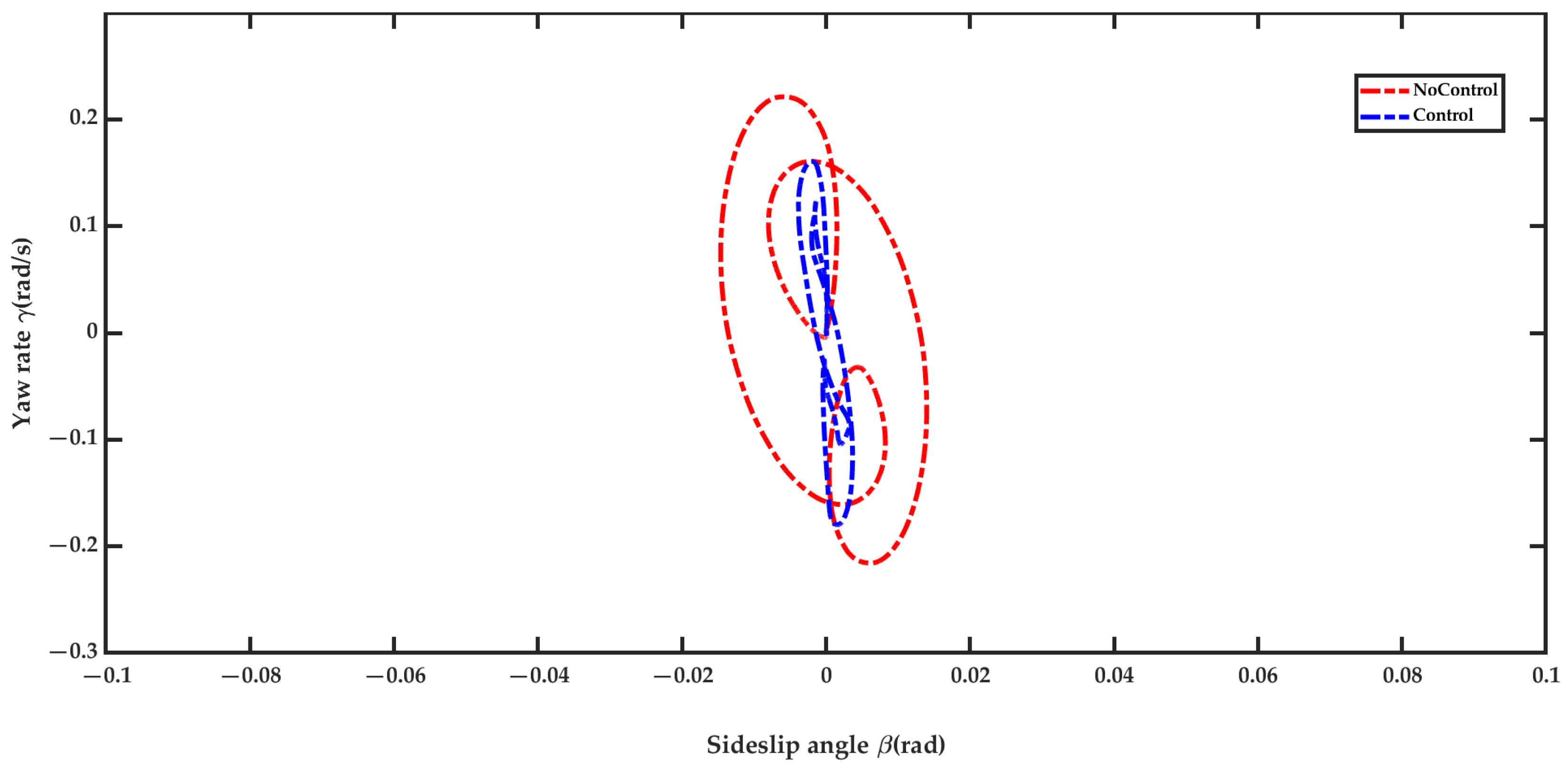
5.2. Result Analysis

Operating Condition 1.
v x = 60   km / h , μ = 0.5 . Controller parameters: k 1 = 12 , k 2 = 12 , ± k c 1 = ± arctan ( 0.02   μ g ) , ± k c 2 = ± 0.85 ( μ g / ν x ) , ξ = 0.5 , ω n = 1000 . The simulation results are shown in Figure 5, Figure 6, Figure 7, Figure 8, Figure 9 and Figure 10.
Under the double-lane change front-wheel steering input condition shown in Figure 5, the peak absolute value of the front-wheel steering angle reaches 0.075   rad . As observed in Figure 6, under the control of the proposed controller, the vehicle’s centroid sideslip angle effectively tracks the desired value. During the lane-change process, when the front-wheel steering angle returns to neutral, the vehicle state variables remain well below their constraint boundaries, k c 1 and k c 1 . Compared to the desired value, the standard deviation is only 0.001   rad . In contrast, in the uncontrolled case, although the variation in the centroid sideslip angle also remains far below the constraint boundary, the standard deviation increases to 0.0041   rad , indicating significantly larger fluctuations than in the controlled scenario. As shown in Figure 7, the analysis of the yaw rate reveals that, in the absence of control, as the front-wheel steering angle increases, the yaw rate gradually approaches its constraint boundary of 0.253   rad / s , with a maximum peak value of 0.2211   rad / s , suggesting a potential instability risk under emergency lane-change conditions. However, with the controller in effect, the peak yaw rate is reduced to 0.1798   rad / s , which is well below the constraint boundaries k c 2 and k c 2 , significantly reducing yaw rate fluctuations and improving the vehicle’s stability margin.
Operating Condition 2.
v x = 90   km / h , μ = 0.85 . The simulation results are shown in Figure 11, Figure 12, Figure 13, Figure 14 and Figure 15.
In Driving Condition 2, the front-wheel steering angle input remains consistent with that in Driving Condition 1. As shown in Figure 11, regardless of whether the controller is applied, the vehicle state variables remain below their constraint boundaries, k c 1 and k c 1 , during the lane-change process when the front-wheel steering angle returns to neutral. However, in the uncontrolled case, the standard deviation of the centroid sideslip angle reaches 0.0113   rad , which is significantly larger than the 0.0028   rad observed under control, indicating that the controller effectively reduces the fluctuation amplitude of the sideslip angle. Regarding the yaw rate, as observed in Figure 12, in the absence of control, when the front-wheel steering angle is large, the yaw rate closely approaches its constraint boundary, with a maximum peak value of 0.2587   rad / s , indicating a high risk of instability. In contrast, under the controller’s influence, although some fluctuations in the yaw rate persist throughout the process, they remain constrained within the stability range defined by k c 2 and k c 2 , with the maximum peak value reduced to 0.1093   rad / s .
As observed in Figure 8, Figure 9 and Figure 10 and Figure 13, Figure 14 and Figure 15, the stable region of the phase plane for vehicle sideslip angle and yaw rate gradually expands with increasing vehicle speed and road surface adhesion coefficient. Simultaneously, the additional yaw moment and the braking torques of individual wheels also increase accordingly. However, in Driving Condition 1, after the controller intervention, the braking torque fluctuations are more pronounced compared to Driving Condition 2. This phenomenon partially reveals that under low-adhesion conditions, where the peak tire–road friction force is lower, the tires are more prone to entering the saturation region, making it difficult to maintain stable braking torque. This observation aligns well with the actual vehicle driving characteristics.
The simulation results of operating conditions 1 and 2 show that the lateral handling stability command filtering control strategy based on time-varying full-state constraints can effectively constrain the state variables x i i = 1 , 2 within the tight sets Ω x = k d i < x i < k c i , i = 1 , 2 . This validates the correctness and effectiveness of the proposed control algorithm. Compared to the uncontrolled case, the proposed control strategy significantly enhances vehicle yaw stability.

6. Conclusions

This paper focuses on the research of vehicle yaw stability control and proposes a lateral handling stability command filtering control method considering time-varying full-state constraints. By introducing a TS-BLF, the proposed approach effectively constrains two key state variables—the centroid sideslip angle and yaw rate—thereby enhancing system stability and safety. Meanwhile, command filtering technology is employed to reduce computational complexity, and an error compensation mechanism is integrated to further optimize the dynamic response, mitigating the adverse effects of filter-induced errors on system performance. To validate the effectiveness and robustness of the proposed control method, simulations were conducted under two different road conditions and vehicle speeds. The results demonstrate that this approach significantly improves the system’s stability margin, providing valuable theoretical support and reference for vehicle safety design. However, this method has limited capability in handling uncertainties and unknown disturbances. As a next step, we plan to integrate robust control algorithms to further enhance the adaptability of the control strategy to complex and dynamic environments, thereby improving its suitability for engineering applications.

Author Contributions

D.Z. conceived the research idea and developed the implementation methodology. L.W. drafted the manuscript, reviewed and edited it, verified the experimental process and results, and conducted parts of the experiments. All authors have read and agreed to the published version of the manuscript.

Funding

This study was supported by Project E2024203257.

Data Availability Statement

Due to the nature of this research, participants in this study did not agree for their data to be shared publicly, so supporting data are not available.

Conflicts of Interest

The authors declare no conflicts of interest.

References

  1. Jeong, E.; Cheol, O. Evaluating the effectiveness of active vehicle safety systems. Accid. Anal. Prev. 2017, 100, 85–96. [Google Scholar] [PubMed]
  2. Song, C.; Xuan, S.; Li, J.; Jin, L. Research on Vehicle Electronic Stability Control Method. In Proceedings of the 2010 2nd International Workshop on Intelligent Systems and Applications, Wuhan, China, 22–23 May 2010. [Google Scholar]
  3. Hu, J.; Wang, Y.; Fujimoto, H.; Hori, Y. Robust yaw stability control for in-wheel motor electric vehicles. IEEE/ASME Trans. Mechatron. 2017, 22, 1360–1370. [Google Scholar] [CrossRef]
  4. Hang, P.; Xia, X.; Chen, X. Handling stability advancement with 4WS and DYC coordinated control: A gain-scheduled robust control approach. IEEE Trans. Veh. Technol. 2021, 70, 3164–3174. [Google Scholar]
  5. Li, Z.; Jiao, X.; Zhang, T. Robust H∞ Output Feedback Trajectory Tracking Control for Steer-by-Wire Four-Wheel Independent Actuated Electric Vehicles. World Electr. Veh. J. 2023, 14, 147. [Google Scholar] [CrossRef]
  6. Ge, P.; Guo, L.; Feng, J.; Zhou, X. Adaptive Stability Control Based on Sliding Model Control for BEVs Driven by In-Wheel Motors. Sustainability 2023, 15, 8660. [Google Scholar] [CrossRef]
  7. Chen, L.; Tang, L. Yaw stability control for steer-by-wire vehicle based on radial basis network and terminal sliding mode theory. Proc. Inst. Mech. Eng. Part D J. Automob. Eng. 2023, 237, 2036–2048. [Google Scholar]
  8. Chen, Y.; Cheng, Q.; Gan, H.; Hao, X. Lateral Stability Control of a Distributed Electric Vehicle Using a New Sliding Mode Controler. Int. J. Automot. Technol. 2023, 24, 1089–1100. [Google Scholar] [CrossRef]
  9. Silva, F.; Silva, L.; Eckert, J.; Yamashita, R.; Lourenço, M. Parameter influence analysis in an optimized fuzzy stability control for a four-wheel independent-drive electric vehicle. Control Eng. Pract. 2022, 120, 105000. [Google Scholar] [CrossRef]
  10. Geng, G.; Cheng, P.; Sun, L.; Xu, X.; Shen, F. A Study on Lateral Stability Control of Distributed Drive Electric Vehicle Based on Fuzzy Adaptive Sliding Mode Control. Int. J. Automot. Technol. 2024, 25, 1415–1429. [Google Scholar] [CrossRef]
  11. Cao, Y.; Xie, Z.; Li, W.; Wang, X.; Wong, P.; Zhao, J. Combined Path Following and Direct Yaw-Moment Control for Unmanned Electric Vehicles Based on Event-Triggered T–S Fuzzy Method. Int. J. Fuzzy Syst. 2024, 26, 2433–2448. [Google Scholar] [CrossRef]
  12. Ileš, Š.; Švec, M.; Makarun, P.; Hromatko, J. Predictive direct yaw moment control with active steering based on polytopic linear parameter-varying model. In Proceedings of the 2022 8th International Conference on Control, Decision and Information Technologies (CoDIT), Istanbul, Turkey, 17–20 May 2022. [Google Scholar]
  13. Rini, G.; Mazzilli, V.; Bottiglione, F.; Gruber, P.; Dhaens, M.; Sorniotti, A. On Nonlinear Model Predictive Vehicle Dynamics Control for Multi-Actuated Car-Semitrailer Configurations. IEEE Access 2024, 12, 165928–165947. [Google Scholar] [CrossRef]
  14. Guo, N.; Lenzo, B.; Zhang, X.; Zou, Y.; Zhai, R.; Zhang, T. A Real-Time Nonlinear Model Predictive Controller for Yaw Motion Optimization of Distributed Drive Electric Vehicles. IEEE Trans. Veh. Technol. 2020, 69, 4935–4946. [Google Scholar] [CrossRef]
  15. Tee, K.; Ge, S.; Tay, E. Barrier Lyapunov functions for the control of output-constrained nonlinear systems. Automatica 2009, 45, 918–927. [Google Scholar] [CrossRef]
  16. Li, H.; Luo, P.; Li, Z.; Zhu, G.; Zhang, X. Finite Time-Adaptive Full-State Quantitative Control of Quadrotor Aircraft and QDrone Experimental Platform Verification. Drones 2024, 8, 351. [Google Scholar] [CrossRef]
  17. Kim, S.; Kim, M.; Kim, Y. Fault-Tolerant Adaptive Control for Trajectory Tracking of a Quadrotor Considering State Constraints and Input Saturation. IEEE Trans. Aerosp. Electron. Syst. 2024, 60, 3148–3159. [Google Scholar] [CrossRef]
  18. Wang, C.; Yang, N.; Li, W.; Liang, M. Event-Triggered Finite-Time Fuzzy Tracking Control for a Time-Varying State Constrained Quadrotor System based on Disturbance Observer. Aerosp. Sci. Technol. 2024, 151, 109329. [Google Scholar] [CrossRef]
  19. Xu, F.; Tang, L.; Liu, Y. Tangent barrier Lyapunov function-based constrained control of flexible manipulator system with actuator failure. Int. J. Robust Nonlinear Control 2021, 31, 8523–8536. [Google Scholar] [CrossRef]
  20. Zhang, X.; Li, Y. Adaptive neural boundary control for state constrained flexible manipulators. Int. J. Adapt. Control Signal Process. 2023, 37, 2184–2203. [Google Scholar] [CrossRef]
  21. Li, Q.; Mei, K. A state-constrained second-order sliding mode control for permanent magnet synchronous motor drives. Nonlinear Dyn. 2024, 112, 12269–12282. [Google Scholar] [CrossRef]
  22. Jiang, Q.; Ma, Y.; Liu, J.; Yu, J. Full state constraints-based adaptive fuzzy finite-time command filtered control for permanent magnet synchronous motor stochastic systems. Int. J. Control Autom. Syst. 2022, 20, 2543–2553. [Google Scholar] [CrossRef]
  23. Dai, B.; Wang, Z. Disturbance observer-based sliding mode control using barrier function for output speed fluctuation constraints of PMSM. IEEE Trans. Energy Convers. 2024, 39, 1192–1201. [Google Scholar] [CrossRef]
  24. Cao, Z.; Mao, J.; Zhang, C.; Cui, C.; Yang, J. Safety-Critical Generalized Predictive Control for Speed Regulation of PMSM Drives Based on Dynamic Robust Control Barrier Function. IEEE Trans. Ind. Electron. 2024, 72, 1881–1891. [Google Scholar] [CrossRef]
  25. Farrell, J.; Polycarpou, M.; Sharma, M.; Dong, W. Command filtered backstepping. IEEE Trans. Autom. 2009, 54, 1391–1395. [Google Scholar] [CrossRef]
  26. Zhou, Y.; Wang, X.; Xu, R. Command-filter-based adaptive neural tracking control for a class of nonlinear MIMO state-constrained systems with input delay and saturation. Neural Netw. 2022, 147, 152–162. [Google Scholar] [CrossRef] [PubMed]
  27. Chen, L.; Chen, F.; Fang, J. Command filter-based adaptive finite-time control of fractional-order nonlinear constrained systems with input saturation. Asian J. Control, 2024; online version of record. [Google Scholar] [CrossRef]
  28. Zhang, Y.; Lei, Y.; Zhang, T.; Song, R.; Li, Y.; Du, F. Robust Command-Filtered Control With Prescribed Performance for Flexible-Joint Robots. IEEE Trans. Instrum. Meas. 2023, 72, 7506013. [Google Scholar] [CrossRef]
  29. Wu, L.; Liu, Z.; Zhao, D. Command-Filtered Yaw Stability Control of Vehicles with State Constraints. Actuators 2025, 14, 148. [Google Scholar] [CrossRef]
  30. Gao, M.; Li, J.; Hu, T.; Luo, J.; Feng, B. Intelligent vehicle trajectory tracking with an adaptive robust nonsingular fast terminal sliding mode control in complex scenarios. Sci. Rep. 2024, 14, 31085. [Google Scholar] [CrossRef]
  31. Dugoff, H.; Fancher, P.; Segel, L. An analysis of tire traction properties and their influence on vehicle dynamic performance. SAE Trans. 1970, 79, 1219–1243. [Google Scholar] [CrossRef]
  32. Zhang, L.; Yan, T.; Pan, F.; Ge, W.; Kong, W. Research on direct yaw moment control of electric vehicles based on Electrohydraulic Joint Action. Sustainability 2022, 14, 11072. [Google Scholar] [CrossRef]
  33. Li, H.; Wang, K.; Hao, H.; Wu, Z. Yaw Moment Control Based on Brake-by-Wire for Vehicle Stbility. World Electr. Veh. J. 2023, 14, 256. [Google Scholar] [CrossRef]
  34. Masato, A. Vehicle Handling Dynamics: Theory and Application; Butterworth-Heinemann: Oxford, UK, 2015. [Google Scholar]
  35. Ren, B.; Ge, S.; Tee, K.; Lee, T. Adaptive Neural Control for Output Feedback Nonlinear Systems Using a Barrier Lyapunov Function. IEEE Trans. Neural Netw. 2010, 21, 1339–1345. [Google Scholar] [PubMed]
  36. Yu, J.; Zhao, L.; Yu, H.; Lin, C. Barrier Lyapunov functions-based command filtered output feedback control for full-state constrained nonlinear systems. Automatica 2019, 105, 71–79. [Google Scholar]
  37. Cui, G.; Xu, S.; Zhang, B.; Lu, J.; Li, Z.; Zhang, Z. Adaptive tracking control for uncertain switched stochastic nonlinear pure-feedback systems with unknown backlash-like hysteresis. J. Frankl. Inst. 2017, 354, 1801–1818. [Google Scholar] [CrossRef]
  38. Yu, J.; Shi, P.; Zhao, L. Finite-time command filtered backstepping control for a class of nonlinear systems. Automatica 2018, 92, 173–180. [Google Scholar]
  39. Liang, J.; Feng, J.; Lu, Y.; Yin, G.; Zhuang, W.; Mao, X. A direct yaw moment control framework through robust TS fuzzy approach considering vehicle stability margin. IEEE/ASME Trans. Mechatron. 2023, 29, 166–178. [Google Scholar]
  40. Chen, J.; Liu, Y.; Liu, R.; Xiao, F.; Huang, J. Integrated control of braking-yaw-roll stability under steering-braking conditions. Sci. Rep. 2023, 13, 21110. [Google Scholar]
  41. Muhammad, E.; Vali, A.; Kashaninia, A.; Behnamgol, V. Coordination of Active Front Steering and Direct Yaw Control Systems Using MIMO Sliding Mode Control. Int. J. Control Autom. Syst. 2024, 22, 1–15. [Google Scholar] [CrossRef]
Figure 1. Vehicle Lateral Handling Stability Control Process.
Mathematics 13 01217 g001
Figure 2. 2-DOF Model.
Mathematics 13 01217 g002
Figure 3. Structure of the second-order command filter.
Mathematics 13 01217 g003
Figure 4. Logarithmic Barrier Lyapunov Function.
Mathematics 13 01217 g004
Figure 5. Front wheel steering angle δ f .
Mathematics 13 01217 g005
Figure 6. Sideslip angle β .
Mathematics 13 01217 g006
Figure 7. Yaw rate γ .
Mathematics 13 01217 g007
Figure 8. Phase plane representation of the vehicle’s sideslip angle and yaw rate.
Mathematics 13 01217 g008
Figure 9. Additional yaw moment.
Mathematics 13 01217 g009
Figure 10. Braking torques of the four wheels.
Mathematics 13 01217 g010
Figure 11. Sideslip angle β .
Mathematics 13 01217 g011
Figure 12. Yaw rate γ .
Mathematics 13 01217 g012
Figure 13. Phase plane representation of the vehicle’s sideslip angle and yaw rate.
Mathematics 13 01217 g013
Figure 14. Additional yaw moment.
Mathematics 13 01217 g014
Figure 15. Braking torques of the four wheels.
Mathematics 13 01217 g015
Disclaimer/Publisher’s Note: The statements, opinions and data contained in all publications are solely those of the individual author(s) and contributor(s) and not of MDPI and/or the editor(s). MDPI and/or the editor(s) disclaim responsibility for any injury to people or property resulting from any ideas, methods, instructions or products referred to in the content.

