Modeling of Must Fermentation Processes for Enabling CO₂ Rate-Based Control

Abstract

Models for must fermentation kinetics are investigated and used in simulations for enabling control strategies based on temperature adjustment during the alcoholic fermentation process using the estimated CO₂ rate. An acoustic emission digital processing approach for estimating the CO₂ rate in the must fermentation process is proposed and investigated. The hardware architecture was designed considering easy integration with other sensor networks, remote monitoring of the fermentation-related parameters, and wireless communication between the fermentation vessel and the processing unit. It includes a virtual CO₂ rate sensor, having as input the audio signal collected by a microphone and as output the estimated CO₂ rate. Digital signal processing performed on an embedded board involves acquisition, filtering, analysis, and feature extraction. Time domain-based methods for analyzing the audio signal were implemented. An experimental setup with a small fermentation vessel (100 L) was used for CO₂ rate monitoring during the fermentation of grape must. The estimated CO₂ rate data were fitted with the CO₂ rate profiles generated by simulating the models under similar conditions. Simulations for controlling fermentation kinetics through a CO₂ rate-based temperature control were performed and analyzed. The simulations indicate the proposed approach as valid for a closed-loop system implementation capable of controlling kinetics behavior using estimated CO₂ rate and temperature control.

1. Introduction

Wine fermentation involves the metabolism of glucose and fructose to ethanol via glycolysis; the primary end product of this process is ethanol. It is important to emphasize that the additional yeast metabolites are responsible for wine’s fragrance, as they donate the basic aromatic attributes of wine. It is well recognized that adjustments in primary and secondary yeast metabolism are definitive for wine qualities.

The fermentation process associated with the alcoholic fermentation in wine production is a very complex process. Various factors influence its dynamics, playing a crucial role in the wine production process. This procedure is essential as it directs wine development to achieve the specific qualities sought by the enologist or the attributes preferred by the target consumers. Controlling the behavior of this process is crucial, as its fine-tuning should permit the seamless production of premium wines. It is already demonstrated that real-time monitoring of fermentation is enabling the rapid detection of developing problems and implementation of required remedial actions [1].

CO₂ is an important factor in different phases of wine production. During the must fermentation phase, CO₂ is released in the form of bubbles as the yeast converts the sugar in the grapes into alcohol. CO₂ rate is highly correlated with the temperature of the fermenting liquid.

During the maturation phase, monitoring of CO₂ and oxygen helps in preventing undesired CO₂ losses and oxidation that may be caused by leaking storage tanks. Before bottling, the dissolved CO₂ level influences the taste and smell of the wine [2].

This paper proposes an approach for estimating the CO₂ rate in the must fermentation phase based on the acoustic emissions produced by CO₂ bubbling. As microorganisms metabolize sugars, CO₂ is produced as a byproduct. Initially, the CO₂ dissolves in the fermentation medium; however, as saturation levels increase, it begins to form gas bubbles that rise to the surface and escape into the air. The acoustic signals generated are a result of the physical interactions between the CO₂ gas bubbles and the surrounding liquid medium. The use of CO₂ bubblers can enhance the detectability of acoustic signals. As CO₂ passes through the liquid in the bubbler, it forms gas bubbles that rise to the surface and burst, releasing energy in the form of sound waves. The liquid in the bubbler serves as a resonator, amplifying the sound profile of the bubbles. Consequently, a CO₂ bubbler can be regarded as a natural acoustic transducer, converting microbial gas production into measurable sound patterns. CO₂ monitoring using bubblers represents a simple, reliable, and cost-effective method. By counting bubble frequency, the rate of fermentation can be inferred. This provides valuable information that allows winemakers to make real-time adjustments on key variables such as fermentation temperature and nutrient availability based on CO₂ activity to protect and enhance aromatic compounds. This method circumvents the need for costly biochemical analyses or cell-level resolution, making it particularly appealing for winemakers who prioritize aroma expression over detailed microbial profiling. Usage of external microphones for recording acoustic emission signals can be a valuable non-invasive technique for real-time monitoring and analysis of the dynamics of the fermentation process, allowing immediate feedback and adjustments.

Next to CO₂, the must temperature is also an important factor. Too low temperatures (below 18 °C) decrease the yeast growing rate, high temperatures (over 35 °C) may kill the yeast culture, while sudden changes in the temperature can severely affect the yeast [3].

Most of the time, the only direct intervention on the process dynamics that can be performed automatically is the control of must temperature in the fermentation vessel. This is usually achieved in two ways: using an internal heat exchanger submerged in the liquid or using tanks with a double shell. In both cases, a heating or cooling fluid is transported by a controlled pump.

During must fermentation, large volumes of CO₂ are generated (≈260 mL/g glucose) [1]. Thus, the primary information on the kinetics of essential biochemical processes is the CO₂ production rate. The adjustment of temperature through the actuated heat exchangers can serve as a method for maintaining the profiles of the main process variables in the desired bands.

Fermentation time is a critical parameter in winemaking. In industrial winemaking, fermentation time significantly impacts product consistency, production efficiency, and overall profitability. Adjusting the duration of fermentation helps optimize the balance between flavor profile, alcohol content, and phenolic extraction. Shorter fermentation periods enable higher production throughput (more batches per year), reduce energy and labor demands, and minimize the risk of microbial spoilage. On the other hand, extended fermentation times are often employed to enhance the extraction of polyphenols and tannins and to improve aromatic complexity and mouthfeel. In small-scale wineries, fermentation time is often approached with greater flexibility and artisanal focus. Small producers may prioritize flavor development and varietal expression over production speed, opting for longer, more natural fermentations that emphasize complexity and authenticity. Even in this case, continuous monitoring and recording of the temperature and CO₂ production rate are critical for installing a consistent, reproducible set of procedures for this critical stage of wine production.

An optimized fermentation duration preserves volatile aromatics and reduces the risk of sluggish or stuck fermentations. Usage of CO₂ rate profiles as fermentation signatures reflects the metabolic activity of yeast, which is closely tied to the formation of key aromatic compounds.

The paper analyzes and simulates different models in order to validate the architecture of a closed-loop system implementation capable of controlling the kinetics behavior using estimated CO₂ rate and temperature control. The values of the model parameters are sourced from the existing literature and correspond to must fermentation with Saccharomyces cerevisiae, the main yeast used in winemaking due to its greater resistance to high ethanol concentrations. Simulations for maintaining a reference profile for the CO₂ rate in the desired bands by means of proportional control on the temperature are performed.

The experimental setup facilitates acquisition and processing of audio signals related to CO₂ bubbling throughout different stages of must fermentation. The features extracted from the audio signals provide estimated values of the CO₂ production rate on different days of the must fermentation process. These estimates are fitted with the CO₂ rate profiles obtained through simulations under similar conditions.

2. Materials and Methods

2.1. Models for Must Fermentation

Several phases were observed during must fermentation [4]: a latency or lag phase with a duration of a few hours, during which yeast cells adapt to the environmental conditions; an exponential growth phase, during which yeast cell population increases until the maximum number of cells is reached and the assimilable nitrogen is exhausted; a quasi-stationary phase, during which yeast cell population remains almost constant, yeast activity gradually declines (the level of cell viability remains high, typically above 90%, until the sugar is consumed [5]); and a decline phase, during which yeast cells start dying.

Usage of mathematical models for prediction of must fermentation kinetics at different temperatures and initial conditions may prevent problems associated with must fermentation, such as sluggish (sugar utilization completion exceeds 7–10 days [6]) or stuck fermentation (sugar utilization stops and the residual sugar is more than 0.4% weight/volume [6]). Ref. [6] indicates that the primary factors associated with fermentation problems are fermentation temperature and inadequate concentrations of nitrogen.

Various models associated with wine fermentation kinetics are available in the literature [4,5,6,7,8,9,10,11,12,13]. Ref. [7] proposes a combined kinetic model based on the models developed by Coleman, Pizarro, and Scaglia. Ref. [8] analyzes the suitability of previously published wine fermentation models for commercial applications and provides the mathematical description and comparison of three models (extended Boulton model, Coleman model, and the Australian Wine Research Institute (AWRI) model). Ref. [9] states that there are several different factors in the fermentation process of Chinese rice wine compared to other simultaneous saccharification and fermentation processes, introducing an unstructured kinetic model with 12 parameters specific to Chinese rice wine fermentation and analyzing the influence of temperature on cell growth, sugar concentration, ethanol production, and pH.

The mathematical description of two widely cited models introduced by Boulton [10] and Coleman et al. [6], a model developed by Borzi et al. that considers the influence of oxygen on the fermentation kinetics [11], and a model developed by Bartsch et al. [12] that includes the presence of aromas and acids are presented in what follows. The main characteristics of these models are summarized in

Table 1. Main characteristics of the fermentation models.

Model	State Variables	Main Characteristics
Boulton, 1980 [10]	X [g·L−1]—total yeast cell mass (Xv—viable cell mass expressed as f(X,E,t))	considers yeast viability
	S [g·L−1]—sugar concentration	models temperature evolution
	E [g·L−1]—ethanol concentration
	T [K]—temperature
Coleman et al., 2007 [6]	X [g·L−1]—total biomass	models active biomass
	XA [g·L−1]—active biomass	combines ODEs with regression techniques for describing the effect of temperature and initial nitrogen condition on model parameters
	N [mg·L−1]—nitrogen concentration
	E [g·L−1]—ethanol concentration
	S [g·L−1]—sugar concentration
Borzi et al., 2014 [11]	X [g·L−1]—total biomass	includes a death phase for yeast,
	N [g·L−1]—nitrogen concentration	does not cover the lag phase,
	E [g·L−1]—ethanol concentration	considers the influence of oxygen on the fermentation process
	S [g·L−1]—sugar concentration
	O2 [g·L−1]—oxygen concentration
Bartsch et al., 2019 [12]	X [g·L−1]—yeast	models yeast dying behavior,
	Nx, NTr [g·L−1]—concentration of nitrogen components	models oxygen evolution (important for yeast activity; unconsumed oxygen may lead to wine oxidation),
	E [g·L−1]—ethanol concentration
	S [g·L−1]—sugar concentration
	O2 [g·L−1]—oxygen concentration	considers glucose transporters (essential for sugar and nitrogen assimilation),
	Tr [g·L−1]—glucose transporters
	P [g·L−1]—propanol
	A [g·L−1]—isoamyl alcohol	considers the presence of aromas and acids
	B [g·L−1]—isobutanol
	MA [g·L−1]—malic acid
	TA [g·L−1]—tartaric acid
	AA [g·L−1]—acetic acid

.

Boulton model introduced in [10] is a general kinetic model for prediction of fermentation behavior of must that considers the relation between must temperature and metabolic activity of the yeast. The system of ordinary differential equations (ODEs) allows prediction of yeast population growth, sugar utilization rates, alcohol production, and temperature variations:

$$\left\{\begin{array}{l}{\displaystyle \frac{\mathrm{d}X}{\mathrm{d}t}}=\mu {·X}_V\\ {\displaystyle \frac{\mathrm{d}S}{\mathrm{d}t}}=-\mu ·{\displaystyle \frac{X_V}{Y_m}}-m·X_V\\ {\displaystyle \frac{\mathrm{d}E}{\mathrm{d}t}}=-{\displaystyle \frac{92}{180}}·{\displaystyle \frac{\mathrm{d}S}{\mathrm{d}t}}\\ {\displaystyle \frac{\mathrm{d}T}{\mathrm{d}t}}={\displaystyle \frac{∆H}{\rho ·C_p}}·{\displaystyle \frac{\mathrm{d}S}{\mathrm{d}t}}-{\displaystyle \frac{U·A}{\rho ·C_p·V}}·\left(T-T_C\right)\end{array}\right.$$

(1)

where t is the time in hours, X ([g·L⁻¹]) is the total yeast cell mass, X_V ([g·L⁻¹]) is the viable yeast cell mass ($X_V=X·{\displaystyle \frac{\left(1-E·t\right)}{42000}}$), E ([g·L⁻¹]) is the ethanol concentration, S ([g·L⁻¹]) is the sugar concentration, T ([K]) is the must temperature, T_C ([K]) is the temperature of the cooling medium or of the surroundings, U ([cal·h⁻¹·m⁻²·K⁻¹]) is the overall heat transfer coefficient, A ([m²]) is the heat transfer area of the fermentation vessel, V ([m³]) is the volume of must, C_p ([cal·kg⁻¹]) is the heat capacity, ρ ([kg·m⁻³]) is the must density, and $∆H$ ([cal·mol⁻¹]) is the enthalpy of the sugars to ethanol conversion with a generally accepted value of 101.2 kJ·mol⁻¹ [8]. The specific growth rate $\mu$ ([h⁻¹]), in the simplest form, is expressed as $\mu ={\mu }_m{\displaystyle \frac{S}{K_S+S}}$, where ${\mu }_m$ is the maximum specific growth rate and $K_S$ is the saturation constant. Relations that consider the transport of sugar components (glucose and fructose) in the presence of competitive inhibition are also introduced. The maximum specific growth rate is expressed as a function of two exponentials corresponding to the increase/decrease in growth: ${\mu }_m=I_g·e^{\left(\frac{E_{I_g}}{R·T}·\frac{T-T_{0g}}{T_{0g}}\right)}-D_g·e^{\left(\frac{E_{D_g}}{R·T}·\frac{T-T_{0g}}{T_{0g}}\right)}$, $I_g=0.18$ h⁻¹, $D_g=0.0054$ h⁻¹, $E_{I_g}=14.2$ kcal·mol⁻¹, $E_{D_g}=121$ kcal·mol⁻¹, $T_{0g}=300$ K, and R is the universal gas constant. The temperature dependence of the saturation constant is given by the expression: $K_S=K_{S0}·e^{\left(\frac{E_s}{R·T}·\frac{T-T_{0s}}{T_{0s}}\right)}$, $K_{S0}=112$ g·L⁻¹ [13], $E_s=-11$ kcal·mol⁻¹, $T_{0s}=293.3$ K. $Y_m$ is the substrate yield for growth coefficient (ref. [13] indicates values for $Y_m$ parameter of 0.1 g biomass/g substrate), and m is the biomass maintenance coefficient: $m=m_0·e^{\left(\frac{-9000}{R·T}·\frac{T-293.3}{293.3}\right)}$.

Coleman et al. model presented in [6] consists of a system of five ordinary differential equations:

$$\left\{\begin{array}{l}{\displaystyle \frac{\mathrm{d}X}{\mathrm{d}t}}=\mu {·X}_A\\ {\displaystyle \frac{\mathrm{d}{\mathrm{X}}_{\mathrm{A}}}{\mathrm{d}t}}=\mu ·X_A-k_d·X_A\\ {\displaystyle \frac{\mathrm{d}N}{\mathrm{d}t}}=-{\displaystyle \frac{\mu ·X_A}{Y_{X/N}}}\\ {\displaystyle \frac{\mathrm{d}E}{\mathrm{d}t}}=\beta ·X_A\\ {\displaystyle \frac{\mathrm{d}S}{\mathrm{d}t}}=-{\displaystyle \frac{\beta ·X_A}{Y_{E/S}}}\end{array} \right.$$

(2)

The state variables are X [g·L⁻¹]—total biomass or cell concentration, X_A [g·L⁻¹]—active biomass, N [mg·L⁻¹]—nitrogen concentration, E [g·L⁻¹]—ethanol concentration, and S [g·L⁻¹]—sugar concentration.

The parameters $\mu$—specific growth rate of yeast cells, k_d—cell death rate, and $\beta$—rate of sugar utilization per cell are expressed as functions of nitrogen concentration, ethanol concentration, and sugar concentration, respectively:

$$\mu ={\displaystyle \frac{{\mu }_{max}·N}{K_N+N}}$$

(3)

$$k_d=k_d^{\prime }·E$$

(4)

$$\beta ={\displaystyle \frac{{\beta }_{max}·S}{K_S+S}}$$

(5)

where ${\mu }_{max}$ is the maximum specific growth rate, $K_N$ is the Monod constant for nitrogen, $k_d^{\prime }$ describes the sensitivity of yeast to ethanol, ${\beta }_{max}$ is the maximum specific rate of sugar utilization, $K_S$ is the Michaelis–Menten-type constant for sugar utilization, $Y_{X/N}$ is the biomass yield on nitrogen, and $Y_{E/S}$ is the ethanol yield on sugar.

Among these parameters, ref. [6] determined that the growth rate of yeast cells, the sugar utilization rate, and the cell death rate are temperature dependent; the yield coefficient of cell mass to utilized nitrogen $Y_{X/N}$ is significantly influenced by the initial nitrogen concentration, while the other parameters, yield coefficient of ethanol to utilized sugar ($Y_{E/S}$), the Monod constant for nitrogen-limited growth ($K_N$), and the Michaelis–Menten-type constant for sugar transport ($K_S$), vary insignificantly with temperature and with respect to the initial conditions.

The model introduced in [11] includes a phase for yeast cells dying and considers the influence of oxygen on the fermentation process:

$$\left\{\begin{array}{l}{\displaystyle \frac{\mathrm{d}X}{\mathrm{d}t}}={\mu }_{max}\left(T\right)·{\displaystyle \frac{N}{K_N+N}}·{\displaystyle \frac{S}{K_{S_1}+S}}·{\displaystyle \frac{O_2}{K_O+O_2}}·X-\Phi (E)·X\\ {\displaystyle \frac{\mathrm{d}N}{\mathrm{d}t}}=-k_1·{\mu }_{max}\left(T\right)·{\displaystyle \frac{N}{K_N+N}}·{\displaystyle \frac{S}{K_{S_1}+S}}·{\displaystyle \frac{O_2}{K_O+O_2}}·X\\ {\displaystyle \frac{\mathrm{d}E}{\mathrm{d}t}}={\beta }_{max}\left(T\right)·{\displaystyle \frac{S}{K_{S_2}+S}}·{\displaystyle \frac{K_E\left(T\right)}{K_E\left(T\right)+E}}·X\\ {\displaystyle \frac{\mathrm{d}S}{\mathrm{d}t}}=-k_2·{\displaystyle \frac{\mathrm{d}E}{\mathrm{d}t}}-k_3·{\mu }_{max}(T)·{\displaystyle \frac{N}{K_N+N}}·{\displaystyle \frac{S}{K_{S_1}+S}}·{\displaystyle \frac{O_2}{K_O+O_2}}·X\\ {\displaystyle \frac{\mathrm{d}{O}_2}{\mathrm{d}t}}=-k_4·{\mu }_{max}(T)·{\displaystyle \frac{N}{K_N+N}}·{\displaystyle \frac{S}{K_{S_1}+S}}·{\displaystyle \frac{O_2}{K_O+O_2}}·X\end{array}\right.$$

(6)

The state variables are X [g·L⁻¹]—total biomass, N [g·L⁻¹]—nitrogen concentration, E [g·L⁻¹]—ethanol concentration, S [g·L⁻¹]—sugar concentration, and O₂ [g·L⁻¹]—oxygen concentration. The parameters expressed as temperature-dependent functions are $\phi \left(E\right)=\left(0.5+{\displaystyle \frac{1}{\pi }}·\arctan \left(k_{d_1}·\left(E-tol\right)\right)\right)·k_{d_2}·{\left(E-tol\right)}^2$, where tol is the tolerance of the ethanol concentration, and k_d1 and k_d2 are parameters related to the cells’ death due to ethanol concentrations greater than the tolerance tol. ${\mu }_{max}\left(T\right)$ and ${\beta }_{max}\left(T\right)$ are maximum specific growth rates described as ${\mu }_{max}\left(T\right)={\mu }_1·T-{\mu }_2$, and ${\beta }_{max}\left(T\right)={\beta }_1·T-{\beta }_2$, $K_E\left(T\right)$ describes the ethanol inhibition: $K_E\left(T\right)=-K_{E_1}·T+K_{E_2}$. K_S1 and K_S2 are saturation constants associated with sugar, K_N is the saturation constant for nitrogen, K_O represents the Michaelis–Menten half-saturation constant for oxygen, k₁ is the yield coefficient associated with nitrogen, k₂ is the yield coefficient associated with sugar, k₃ is the yield coefficient for the part of sugar used as nutrient for yeast, and k₄ is the yield coefficient for oxygen.

Ref. [12] introduces a model that describes the yeast dying phase in relation to the toxic effect of the alcohol component, considers the presence of glucose transporters (essential for the assimilation of sugar and nitrogen), and includes equations for aroma and acid formation:

$$\{\begin{array}{l}\frac{\mathrm{d}X}{\mathrm{d}t}={\mu }_{max}\left(T\right)·\frac{N_x}{K_x+N_x}·\frac{S}{K_{S_1}+S}·\left(\frac{O_2}{K_O+O_2}+\epsilon \right)·X-k_d·X-\phi \left(\mathsf{\Sigma }\right)·X\\ \frac{\mathrm{d}{N}_x}{\mathrm{d}t}=-k_1·{\mu }_{max}\left(T\right)·\frac{N_x}{K_x+N_x}·\frac{S}{K_{S_1}+S}·\left(\frac{O_2}{K_O+O_2}+\epsilon \right)·X\\ \frac{\mathrm{d}S}{\mathrm{d}t}=-k_2·\frac{\mathrm{d}E}{\mathrm{d}t}-k_3·{\mu }_{max}\left(T\right)·\frac{N_x}{K_{x}X+N_x}·\frac{S}{K_{S_1}+S}·\left(\frac{O_2}{K_O+O_2}+\epsilon \right)·X\\ \frac{\mathrm{d}{O}_2}{\mathrm{d}t}=-k_4·{\mu }_{max}\left(T\right)·\frac{N_x}{K_{x}X+N_x}·\frac{S}{K_{S_1}+S}·\frac{O_2}{K_O+O_2}·X\\ \frac{\mathrm{d}E}{\mathrm{d}t}={\beta }_{max}\left(T\right)·\frac{S}{K_{S_2}+S}·\frac{K_E\left(T\right)}{K_E\left(T\right)+E}·X·\left(1+\mathsf{\Phi }\left(T\right)\right)·T_r\\ \frac{\mathrm{d}{T}_r}{\mathrm{d}t}={\eta }_{max}\left(T\right)·\frac{N_{tr}}{K_{tr}+N_{tr}}·\frac{S}{K_{S_1}+S}·\frac{O_2}{K_O+O_2}·X\\ \frac{\mathrm{d}{N}_{tr}}{\mathrm{d}t}=-k_1^{\prime }·{\eta }_{max}\left(T\right)·\frac{N_{tr}}{K_{tr}+N_{tr}}·\frac{S}{K_{S_1}+S}·\frac{O_2}{K_O+O_2}·X\\ \frac{\mathrm{d}P}{\mathrm{d}t}=k_5·{\mu }_{max}\left(T\right)·\frac{N_x}{K_{x}X+N_x}·\frac{S}{K_{S_1}+S}·\left(\frac{O_2}{K_O+O_2}+\epsilon \right)·X\\ \frac{\mathrm{d}A}{\mathrm{d}t}=k_6·{\beta }_{max}\left(T\right)·\frac{S}{K_{S_3}+S}·\frac{K_E\left(T\right)}{K_E\left(t\right)+E}·X·\left(1+\mathsf{\Phi }\left(T\right)·T_r\right)+k_7·{\mu }_{max}\left(T\right)·\frac{N_x}{K_{x}X+N_x}·\frac{S}{K_{S_1}+S}·\left(\frac{O_2}{K_O+O_2}+\epsilon \right)·X\\ \frac{\mathrm{d}B}{\mathrm{d}t}=k_8·{\beta }_{max}\left(T\right)·\frac{S}{K_{S_4}+S}·\frac{K_E\left(T\right)}{K_E\left(t\right)+E}·X·\left(1+\mathsf{\Phi }\left(T\right)·T_r\right)+k_9·{\mu }_{max}\left(T\right)·\frac{N_x}{K_{x}X+N_x}·\frac{S}{K_{S_1}+S}·\left(\frac{O_2}{K_O+O_2}+\epsilon \right)·X\\ \frac{\mathrm{d}AA}{\mathrm{d}t}=k_{10}·{\theta }_{max}\left(T\right)·{\mu }_{max}\left(T\right)·\frac{N_x}{K_x+N_x}·\frac{S}{K_{S_1}+S}·\frac{O_2}{K_O+O_2}·X+k_{11}·{\xi }_{max}\left(T\right)·\frac{\mathrm{d}E}{\mathrm{d}t}-k_a·AA\\ \frac{\mathrm{d}MA}{\mathrm{d}t}=-k_{12}·{\gamma }_{max}\left(T\right)·\frac{MA}{K_{MA}+MA}·\left(\frac{O_2}{K_O+O_2}+k_m\right)\mathrm{}\\ \frac{\mathrm{d}TA}{\mathrm{d}t}=-k_{13}·{\tilde{\gamma }}_{max}(T)·\frac{TA}{K_{TA}+TA}·\left(\frac{O_2}{K_O+O_2}+k_t\right)\end{array}$$

(7)

The system of ODEs models the time evolution of yeast X ([g·L⁻¹]), ethanol E ([g·L⁻¹]), sugar S ([g·L⁻¹]), oxygen O₂ ([g·L⁻¹]), part of assimilable nitrogen converted into yeast N_x ([g·L⁻¹]), part of nitrogen, N_Tr ([g·L⁻¹]), responsible for the synthesis of the transporters T_r ([g·L⁻¹]), three aroma-related compounds—propanol, P ([g·L⁻¹]), isoamyl alcohol, A ([g·L⁻¹]), and isobutanol, B ([g·L⁻¹])—two wine-related acids—malic acid MA ([g·L⁻¹]) and tartaric acid, TA ([g·L⁻¹])—and a by-product of alcoholic fermentation, a volatile acid, acetic acid AA ([g·L⁻¹]).

The parameters expressed as temperature-dependent functions are ${\beta }_{max}\left(T\right)$ and ${\mu }_{max}\left(T\right)$—functions that specify the specific maximal reaction rates on the given substrate; ${\beta }_{max}\left(T\right)={\beta }_1·T+{\beta }_2$, ${\mu }_{max}\left(T\right)={\mu }_1·T-{\mu }_2$, $\Phi \left(T\right)$—function used in the expression of the ethanol, isoamyl alcohol, and isobutanol for expressing the influence of the glucose transporters on the ethanol production; $\Phi \left(T\right)={\Phi }_1·T-{\Phi }_2$, ${\eta }_{max}\left(T\right)$—function influencing the transporters T_r and the part of nitrogen responsible for the transporters synthesis; ${\eta }_{max}\left(T\right)={\eta }_1·T-{\eta }_2$, $K_E\left(T\right)$—function used in the expression of the ethanol, isoamyl alcohol, and isobutanol; $K_E\left(T\right)=-K_{E_1}·T+K_{E_2}$, $\phi \left(\mathsf{\Sigma }\right)$—function that considers influence of alcohol toxicity on the evolution of yeast; $\phi \left(\mathsf{\Sigma }\right)=\left(0.5+{\displaystyle \frac{1}{\pi }}·\arctan \left(k_{d_1}·\left(\mathsf{\Sigma }-tol\right)\right)\right)·k_{d_2}·{\left(\mathsf{\Sigma }-tol\right)}^2$, where $\mathsf{\Sigma }\left(\mathrm{t}\right)=E\left(t\right)+A\left(t\right)+B\left(t\right)+P\left(t\right)$, ${\theta }_{max}\left(T\right)$, ${\xi }_{max}\left(T\right)$, ${\gamma }_{max}\left(T\right)$ and ${\tilde{\gamma }}_{max}\left(T\right)$ are linear functions of temperature used in the expression of the acetic acid, malic acid, and tartaric acid evolution: ${\theta }_{max}\left(T\right)={\theta }_1·T+{\theta }_2$, ${\xi }_{max}\left(T\right)={\xi }_1·T+{\xi }_2$, ${\gamma }_{max}\left(T\right)={\gamma }_1·T+{\gamma }_2$, ${\tilde{\gamma }}_{max}\left(T\right)={\tilde{\gamma }}_1·T+{\tilde{\gamma }}_2$.

The constant parameters are the stoichiometric coefficients expressed in terms of relative ratios: k_i, i = 1…9, $k_1^{\prime }$ and $k_{d_1}$, $k_{d_2}$; Michaelis–Menten constants expressed in [g·L⁻¹]—K_X, K_S1, K_S2, K_S3, K_S4, K_S5, K_E2, K_O, K_Tr, K_AA, K_MA, K_TA, and K_E1—expressed in [g· (L·min)⁻¹].

The temperature-dependent parameters are tol [g·L⁻¹]—tolerance bound of the alcohol concentration, β₁ [(d°C)⁻¹], β₂ [d⁻¹], µ₁ [(d°C)⁻¹], µ₂ [d⁻¹], Φ₁ [L·(g°C)⁻¹), Φ₂ (L·g⁻¹), η₁ [(d°C)⁻¹], and η₂ [d⁻¹], where d is the time in days.

The CO₂ evolution rate was estimated based on the stoichiometric relation between sugar and CO₂ [8]:

$${\displaystyle \frac{\mathrm{d}{CO}_2}{\mathrm{d}t}}=Y_{CO2/S}·{\displaystyle \frac{\mathrm{d}S}{\mathrm{d}t}}$$

(8)

where $Y_{CO2/S}$ is the CO₂ yield per gram of sugar consumed (1 mole of sugar (180.16 g) produces 2 moles of CO₂ (88 g), $Y_{CO2/S}\approx 0.48$).

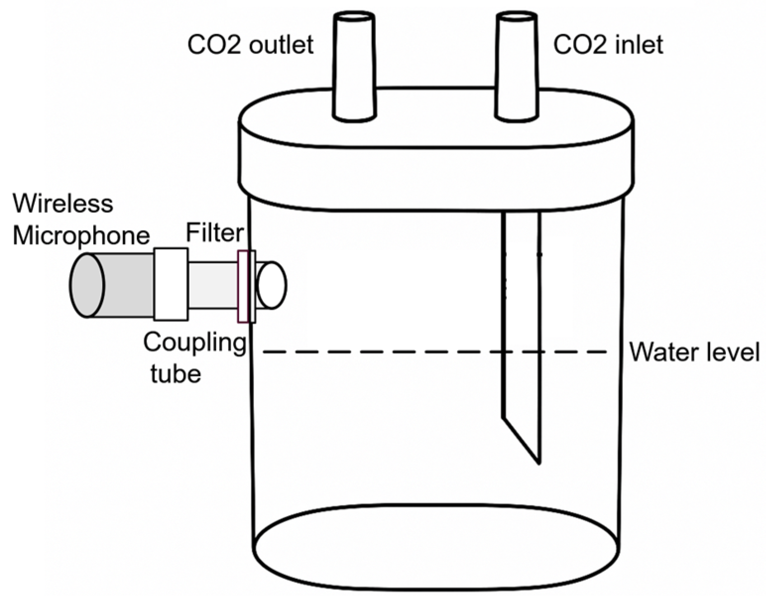
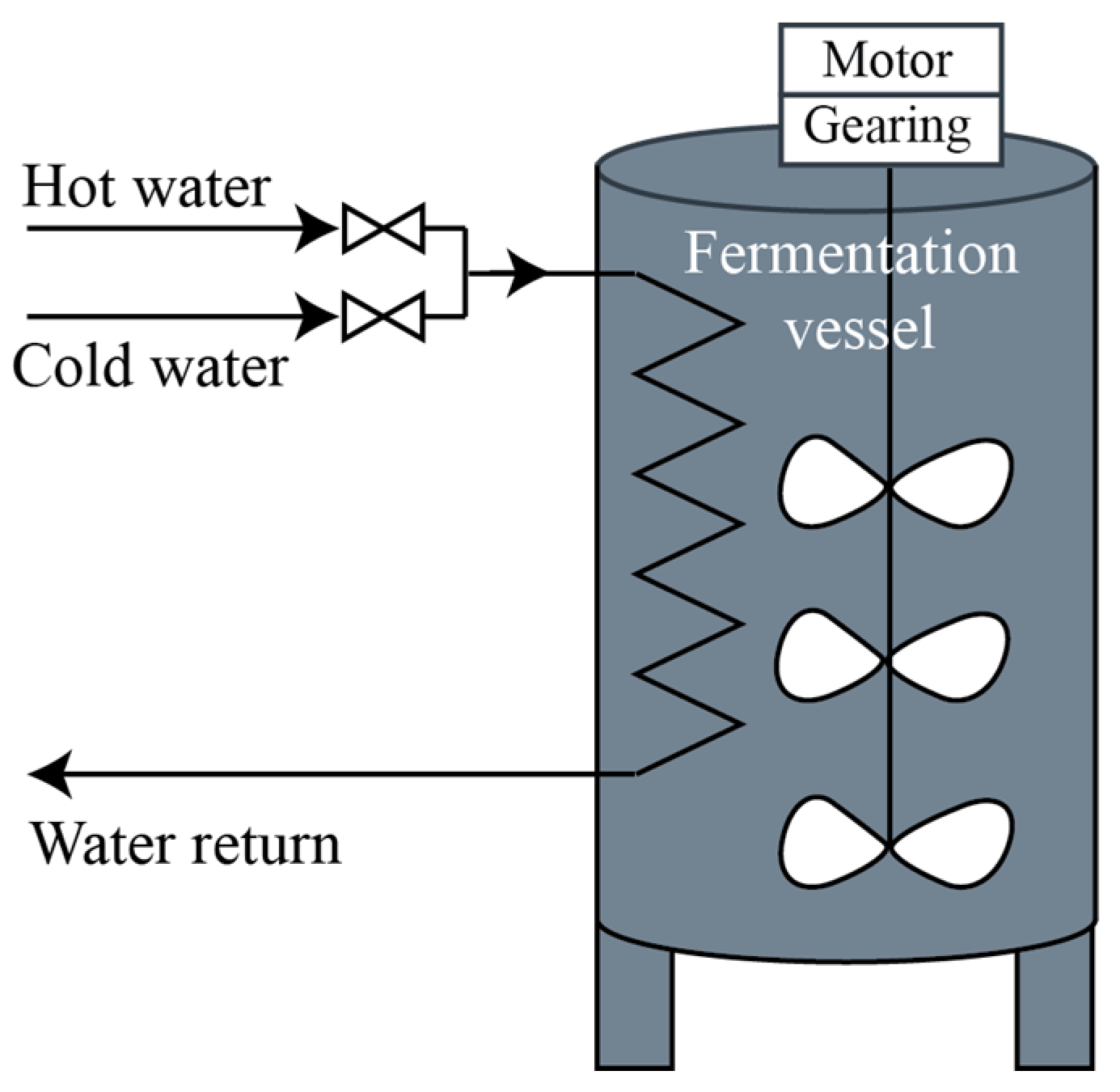
2.2. Experimental Setup for CO₂ Rate Monitoring

The experimental setup is presented in Figure 1. A CO₂ bubbler is attached to the fermentation vessel. A wireless microphone kit connected to an embedded module is used for monitoring the acoustic emissions produced by CO₂. The microcontroller processes the audio signal and transmits the extracted features through a MQTT (Message Queue Telemetry Transport) client. A local MQTT broker with the additional functionality of an MQTT bridge interfaces the system with the cloud.

The microcontroller board is based on a STMicroelectronics Arm Cortex M7 core (STMicroelectronics, headquartered in Geneva, Switzerland) with a frequency that can be configured up to 216 MHz. The memory capacities are as follows: 1 MB of Flash memory, 340 KB of RAM, and 8 MB of accessible SDRAM.

The software development tools employed for configuring the board and implementing the application include STM32CubeMX (version 6.8.1) and STM32CubeIDE (version: 1.12.1). STM32CubeMX is a graphical application designed for the configuration of STM32 microcontrollers and the generation of initialization code in the C programming language. STM32CubeIDE is an IDE (Integrated Development Environment) specifically for STM32, which supports the development and debugging of applications in both C and C++.

The primary considerations for the proposed hardware architecture are easy integration with other sensor networks, remote monitoring of the fermentation-related parameters, and wireless communication between the fermentation vessel and the microcontroller board. The wireless microphone kit communicates on the frequency band VHF (very high frequency)/174 MHz–216 MHz; the maximum communication distance is 30 m. The frequency band of the microphone is 60 Hz–13 KHz (+/−3 db). The setup in Figure 2 illustrates how the microphone is mounted on the CO₂ bubbler for acoustic measurements.

The protocol used for interfacing the virtual CO₂ rate sensor is MQTT, a lightweight and low-bandwidth publish–subscribe messaging protocol, very popular in sensor networks, especially in IoT (Internet of Things) setups. It has a small message overhead, which makes it ideal for devices with limited CPU resources. Devices publish data to topics, and any device subscribed to those topics gets updated automatically, thus decoupling data producers (sensors) from consumers (servers, apps) and making the network more flexible and scalable.

2.3. The Virtual CO₂ Rate Sensor

Figure 3 illustrates the main components of the virtual CO₂ rate sensor. It consists of a microphone connected to an acquisition block capable of converting the analog signal to a digital one. The processing block filters, analysis, and extracts the relevant features from the digital signal (i.e., root mean square value, maximum pulse width, and average frequency) according to the procedure described in Section 2.3.3. The average frequency is used for finding the output of the virtual CO₂ rate sensor, (dCO₂/dt)_est [$\mathrm{g}·{\mathrm{L}}^{-1}·{\mathrm{h}}^{-1}$].

2.3.1. Acoustic Emission Analysis as a Detection Mechanism

Acoustic emission (AE) monitoring and analysis proved to be effective in various applications such as structural health monitoring [14,15], leak detection [16,17], and assessing the condition of machinery [18,19,20]. An acoustic emission method was used in [21] for monitoring the beer fermentation process by means of three piezoelectric sensors placed on the outer side of the fermentation tank. The main parameters considered for processing the acoustic signals were root mean square (RMS) value as an indicator of the amount of energy and power spectral density (PSD) function maximum values as an indicator of the distribution of energy transmitted over the frequency spectrum. The authors concluded that the experiment did not lead to satisfactory results and recommended a detailed study of the fermenter structure and calibration/verification of the sensors.

A sensor array consisting of eight interdigitated chemocapacitors coated with different polymeric materials was used in [22] for monitoring and evaluation of alcoholic fermentation of a typical Greek grape must variety. The sensor responses were compared to those obtained using pure samples or samples contaminated with controlled concentrations of standard ethanol solutions of impurities. Principal component analysis (PCA)-based techniques were used for data processing. The authors concluded that the system could differentiate between a normal grape must fermentation process and a potentially spoiled one.

Two main approaches for monitoring the fermentation process were identified in [3]: (i) usage of piezoelectric sensors attached to the vessel’s wall for monitoring the vibro-acoustic signal and (ii) usage of ultrasonic techniques for detecting changes in the parameters of the fermenting liquid. The study presented in [3] relies on introducing a hydrophone into the fermenting liquid and measuring the CO₂ bubbling process, reducing in this way the effect of interferences associated with the first approach (i), and using a simpler approach compared to (ii). The spectrogram was computed on the data points acquired using a measuring window of 30 s every 30 min. The dominant frequency extracted from each measuring window facilitated the identification of the fermentation stages characteristic of the fermentation process.

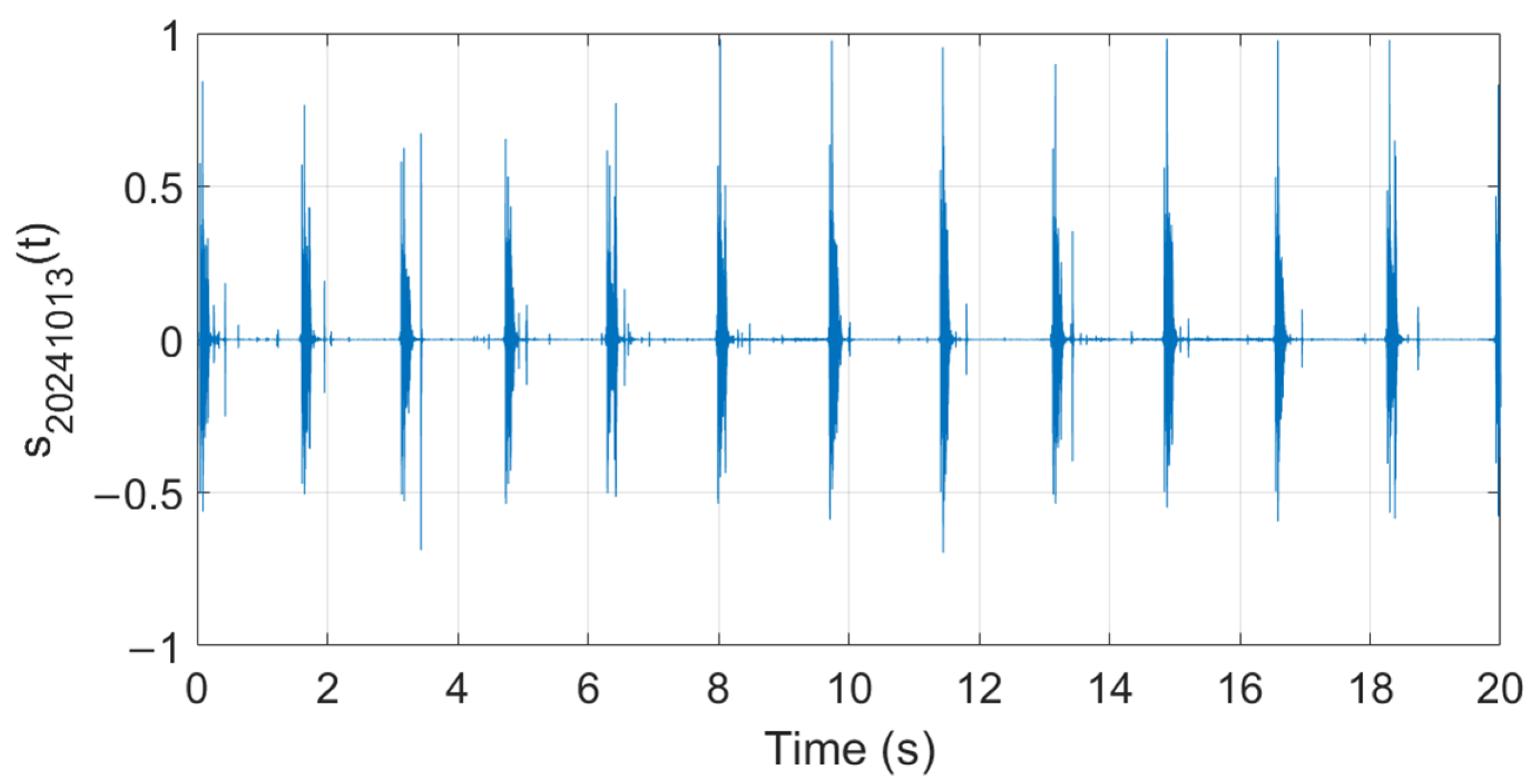
2.3.2. Modeling and Processing of Acoustic Emission Signals

Various approaches for feature extraction and analysis of acoustic emission signals can be found in the literature.

Time domain analysis allows extraction of features like peak and RMS amplitude, crossing rate, event rate, and energy. The work presented in [23] examines AE signals during the first layer manufacturing in the Fused Filament Fabrication process, analyzing raw and RMS values to monitor the process.

Aggregating statistical features of AE signals like mean, variance, skewness, and kurtosis may reveal trends in the analyzed processes. In [24], an artificial neural network model is used for estimating the density of a fermentation mixture. The output was computed based on a set of 11 inputs: speed of sound estimate, temperature, and signal features like spectral centroid, spectral spread, spectral kurtosis, temporal and spectral energy, temporal and spectral crest factor, and temporal and spectral entropy.

Frequency domain analysis provides insights into the processes driving AE signal generation. Features like dominant frequency, frequency bandwidth, and power spectral density may facilitate the distinction between low- and high-frequency events, spread of frequencies, and highlight energy distribution across frequencies. Ref. [25] performs acoustic emission signal analysis in the frequency domain through features like frequency at peak magnitude, median frequency, and percentage signal energy in the frequency band for classification of partial discharges.

Analyzing frequencies over time using transforms like wavelet transform, short-time Fourier transform (STFT), or Hilbert transform may identify abrupt changes, spikes, or transients in signals; track frequency evolution over time; and capture envelope variations over time. In [19], the convolutional neural network model EfficientNet was applied to the images corresponding to the spectrogram of AE signals acquired from bearings for feature extraction and classification of bearing faults.

The work presented in this paper uses time domain-based methods for analyzing signals related to the must fermentation phases, such as RMS value, pulse width, and frequency. In fermentation processes, especially in real-time monitoring and control, it is often not the high-frequency acoustic content of individual bubble bursts that matters most, but rather the frequency of bubble events themselves, which reflects the rate of CO₂ release. During bubble coalescence, multiple small bubbles merge into larger ones, producing complex acoustic signatures, often with clustered pulses or broad energy spikes. These events can be more easily recognized in the RMS envelope, which will show distinct energy envelopes compared to single, isolated bubble bursts. Frequency estimation on the RMS envelope helps capture the temporal spacing and energy distribution of these coalescence events more robustly than analyzing the raw waveform alone.

The RMS value of a signal can be computed either in the time domain ($X_{RMS}=\sqrt{{\displaystyle \frac{1}{N}}{\sum }_{i=1}^N{x}_i^2}$) or in the frequency domain using Parseval’s theorem that relates the energy of a signal in the time domain to its energy in the frequency domain (${\sum }_{i=1}^N{x}_i^2={\displaystyle \frac{1}{N}}{\sum }_{n=1}^N{X}_n^2$, $X_n$ is the discrete Fourier transform of the sequence $x_i$).

For filtering the signals, two low-pass filters were used: a Savitzky–Golay filter and a low-pass FIR filter. The Savitzky–Golay filter [26] is a low-pass filter in the time domain that provides data smoothing without loss of resolution. It uses the assumption that there is a redundancy in the data points that can be used for noise reduction. It works well for data that can be locally fitted by a polynomial, approximating the data within the moving window not by a constant, as in the case of moving window averaging filters, but by a polynomial of higher order. Considering a series of equally spaced data points, $f_i={\left.f\left(t_i\right)\right|}_{t_i=k·∆t}$, each value $f_i$ is replaced by the value of a polynomial of degree M in i ($a_0+a_1·i+a_2·i^2+\cdots +a_M·i^M$, $i=-n_L\dots n_R$). The polynomial coefficients are identified such that higher moments are preserved by least-squares fit the polynomial to the data points in the moving window of length $n_L+n_R+1$. The low-pass filter applied on the RMS envelope is a discrete linear time invariant system whose input-output relationship is described by the linear constant coefficient difference equation [27]: $y_n=b_0·x_n+b_1·x_{n-1}+\cdots +b_N·x_{n-N}$ where b_k are the filter coefficients (samples of the filter impulse response), and $x_n$ are data samples. The coefficients are computed using a least-squares approximation to the desired frequency response, and the impulse response is then smoothed with a Hamming window $w\left[n\right]=0.54-0.46·\cos {\displaystyle \frac{2\pi n}{M}}$.

2.3.3. Digital Signal Processing Algorithm

The procedure applied for extracting the relevant features from the recorded audio signals consists of the following:

• Periodic acquisition of 20 s of audio samples;
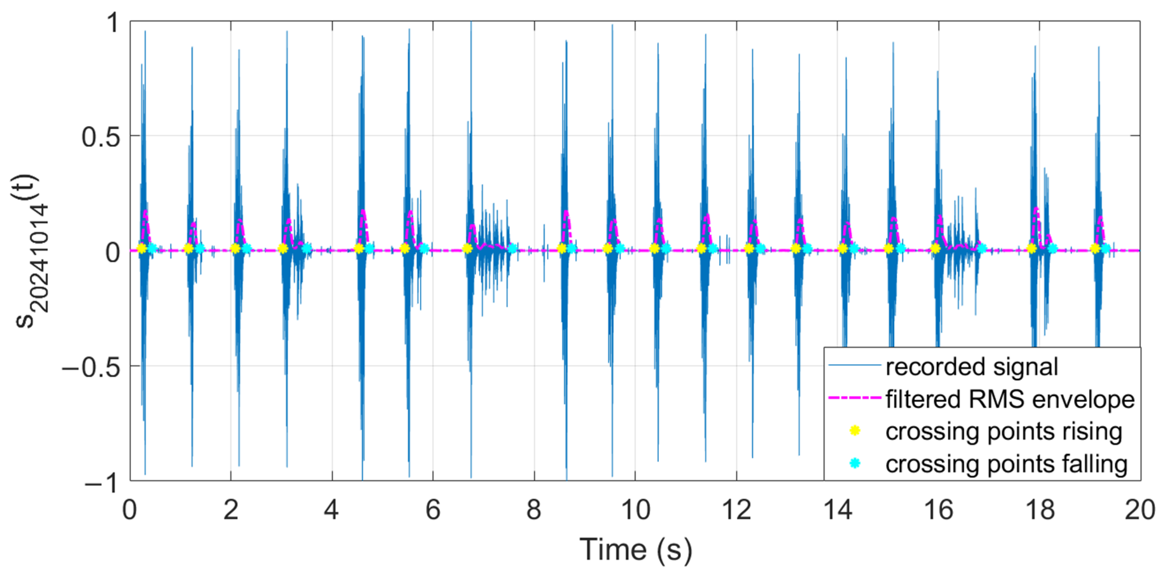
• Filtering the samples using the Savitzky–Golay finite impulse response (FIR) smoothing filter of polynomial order 11 and frame length 255;
• Extraction of upper RMS envelope using a sliding window of length 255;
• Low-pass filtering the extracted envelope (cutting frequency 2 Hz, window size 0.1 s);
• Searching the crossing points using a level of min_val+5%(max_val-min_val), both falling and rising transitions;
• Filtering of the candidate crossing points by removing the points where the distance between falling and raising points is smaller than 20% of the maximum distance between two rising crossing points;
• Extraction of signal parameters like frequency, pulse widths, and RMS value.

The main characteristics considered for analyzing the must fermentation process are as follows:

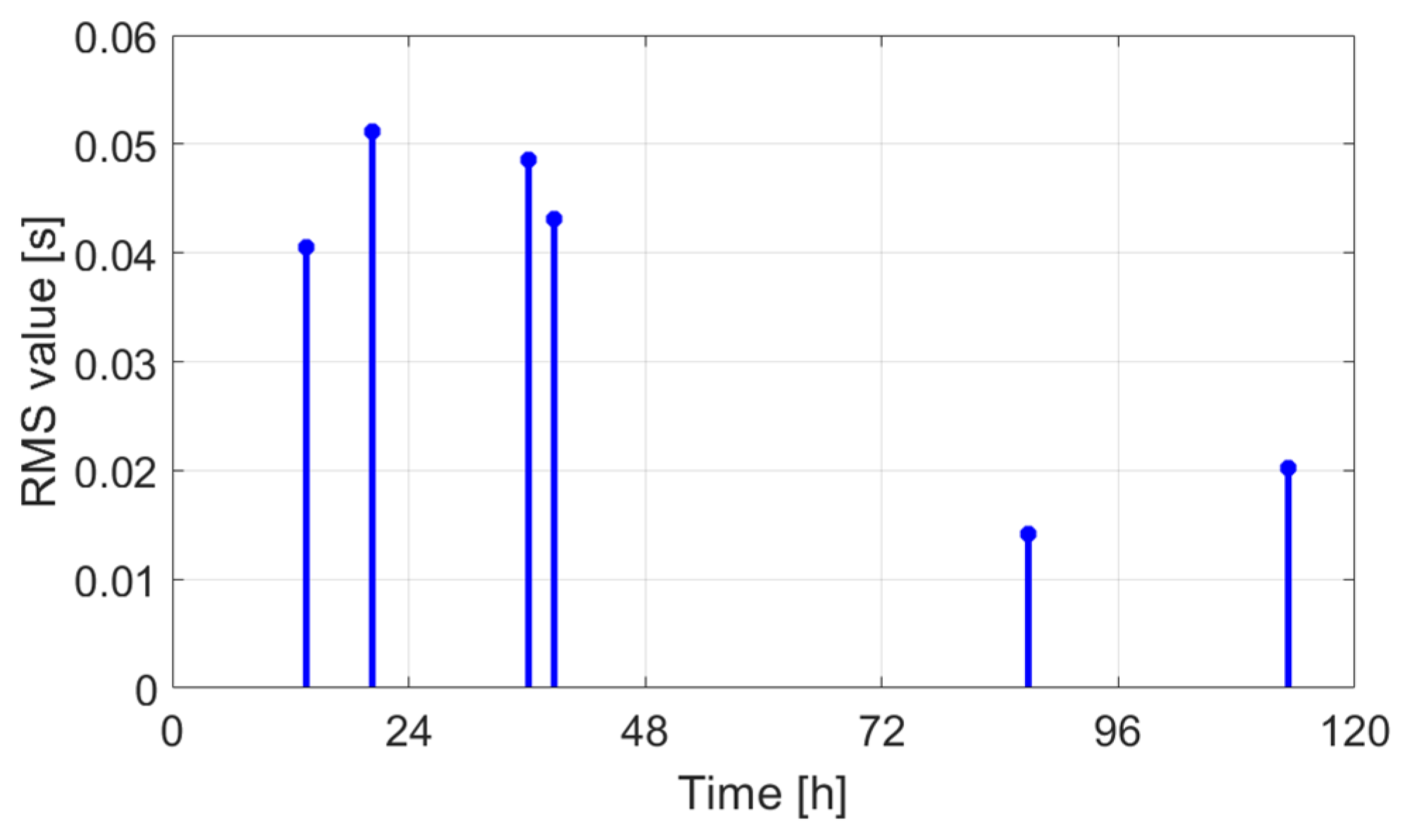
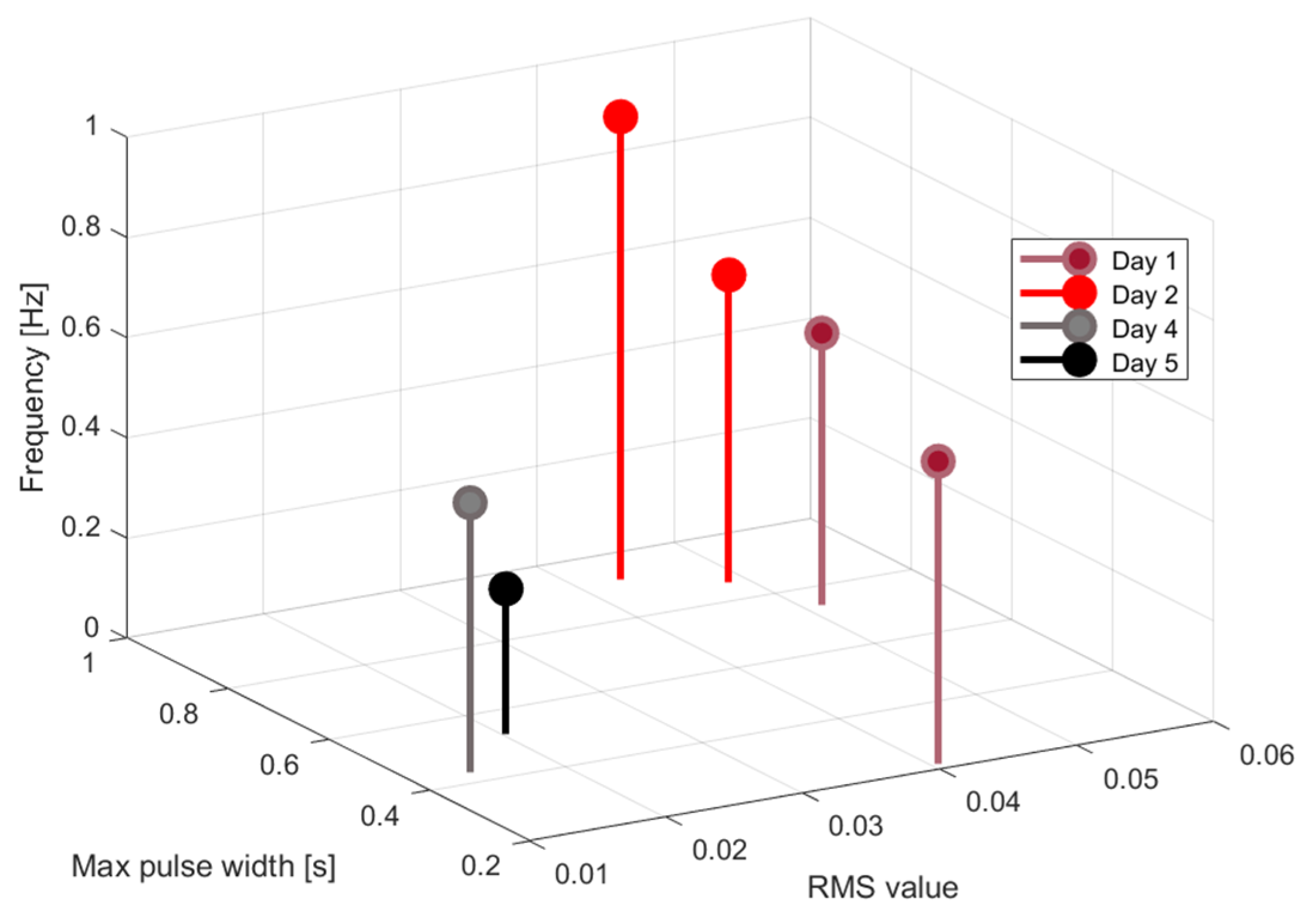
• RMS value, for representing the signal strength, which correlates to fermentation activity (higher RMS values suggest more vigorous activity);
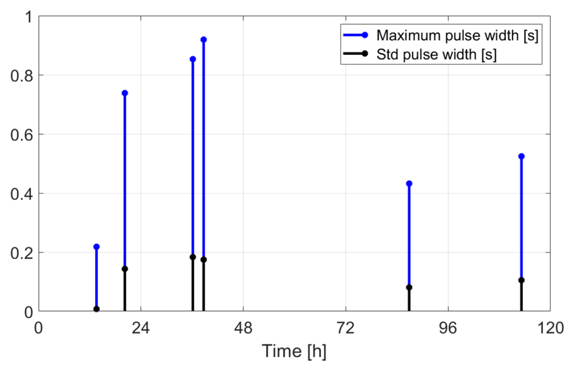
• Maximum pulse width, for indicating the duration of fermentation events, such as CO₂ bubble bursts (longer pulse widths might imply slower, sustained fermentation reactions);
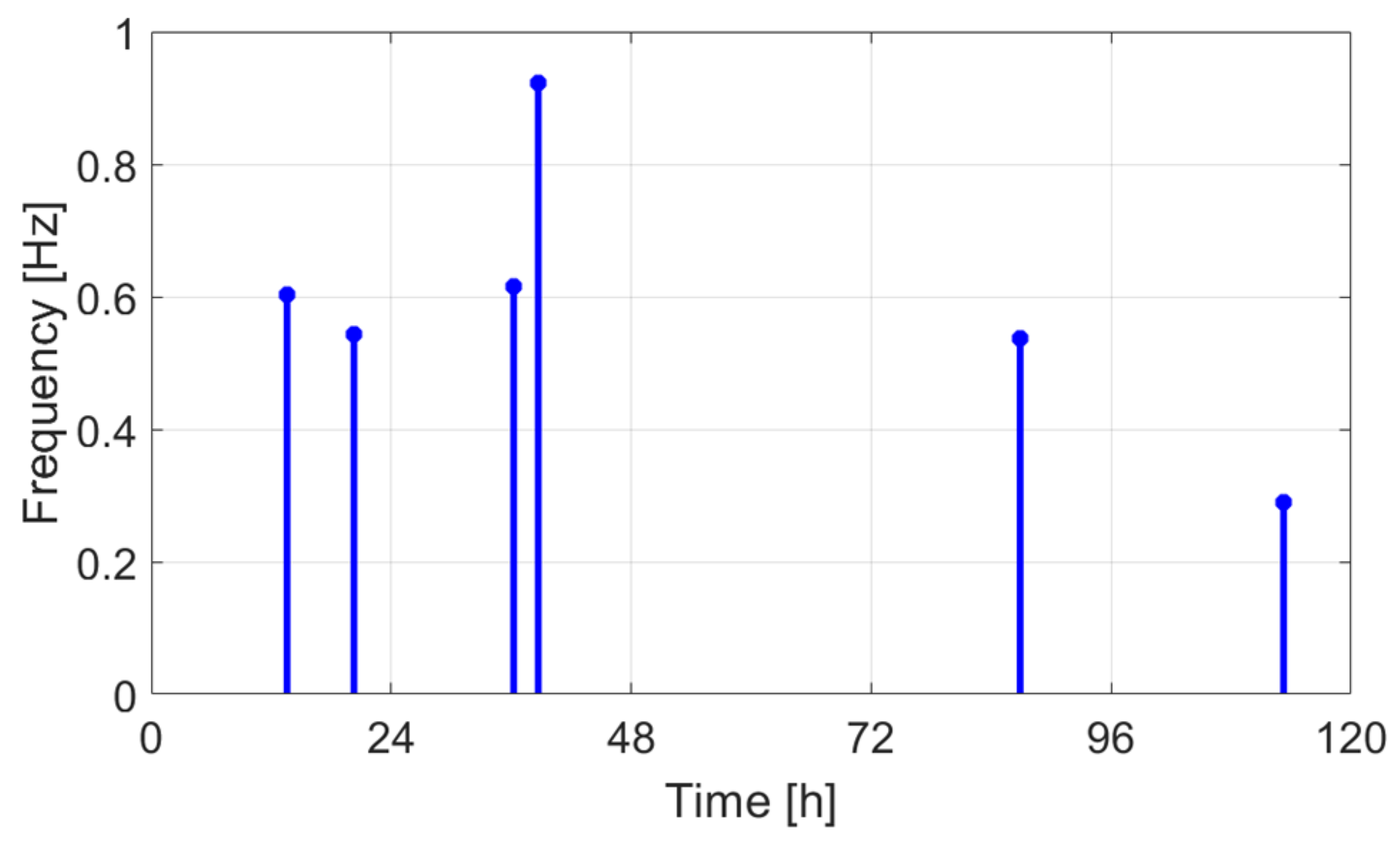
• Average frequency, for observing the periodicity of the events (higher frequencies may indicate faster yeast activity and more CO₂ production).

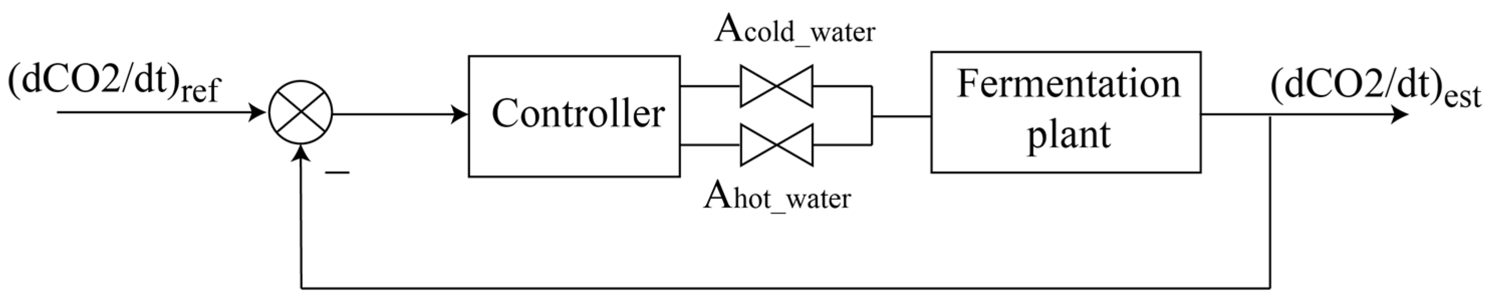
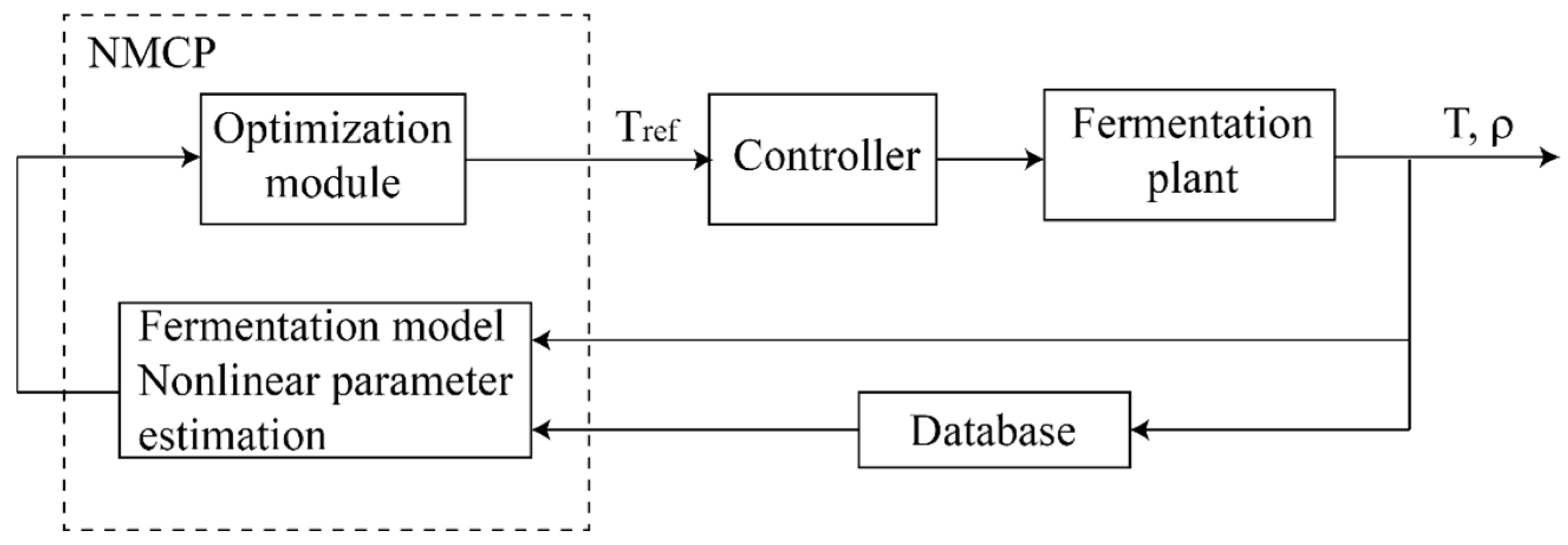
2.4. Control of Must Fermentation Kinetics

Controlling the must fermentation kinetics for a fermentation setup based on a vessel with a heat exchanger and stirring mechanism (Figure 4) can be implemented using a feedback control system like the one illustrated in Figure 5. The CO₂ rate estimated based on the acoustic emission method can be fed back into the system and used in the computation of the controller output signals. In the simplest case of proportional control, the controller’s output, c(t), is computed based on a linear transformation: $c\left(t\right)=k_p·e\left(t\right)+u_0\left(t\right)$, where $e\left(t\right)$ is the difference between the reference value and the controlled variable $k_p$ is the proportional gain factor, and $u_0\left(t\right)$ is the control signal when there is no error.

More advanced control strategies, like the nonlinear model predictive control (NMCP) introduced in [28] (Figure 6), can be implemented for controlling and optimizing the nonlinear process associated with must fermentation.

2.5. Simulation of the Fermentation Models

Coleman et al. model and Boulton model were selected for simulations. The simulations were performed in Matlab Simulink (version R2023a). The Runge–Kutta method with a fixed step size of 1 min was used for the numerical integration of the ODEs. To enhance readability and future scalability, the models implemented in Simulink were built with a modular structure, consisting of interconnected subsystems. Standard integrator blocks were used for the numerical integration of the state variables. To improve clarity and avoid excessive line crossings, From and Goto blocks were used; these blocks allow signals to be passed between components without requiring direct line connections. The choice of these two fermentation models is motivated in what follows.

The kinetics described by Boulton is known as the first wine-specific fermentation model and models the coupled relationships of sugar and nitrogen consumption, ethanol production, and cell death. The must temperature modeling is also considered. A recent literature study [8] validates the extended version of this model as being the most appropriate for commercial wine fermentation. The authors of [8] suggest that, compared to other models in the literature, the extended version provides estimations of must density, accounts for vitamin limitations affecting yeast strain growth, thereby facilitating the characterization of slow and sluggish fermentations, and delivers the most accurate description of fermentation outcomes across all variables. This conclusion is based on experiments conducted on datasets with measurements corresponding to multiple state variables at various temperatures.

Selection of Coleman et al. model was motivated by the study performed by the authors in [6] on describing the effect of temperature and initial nitrogen condition on model parameters. The authors combined the kinetics model with regression techniques and provided profiles for the parameters as functions of temperature and initial values.

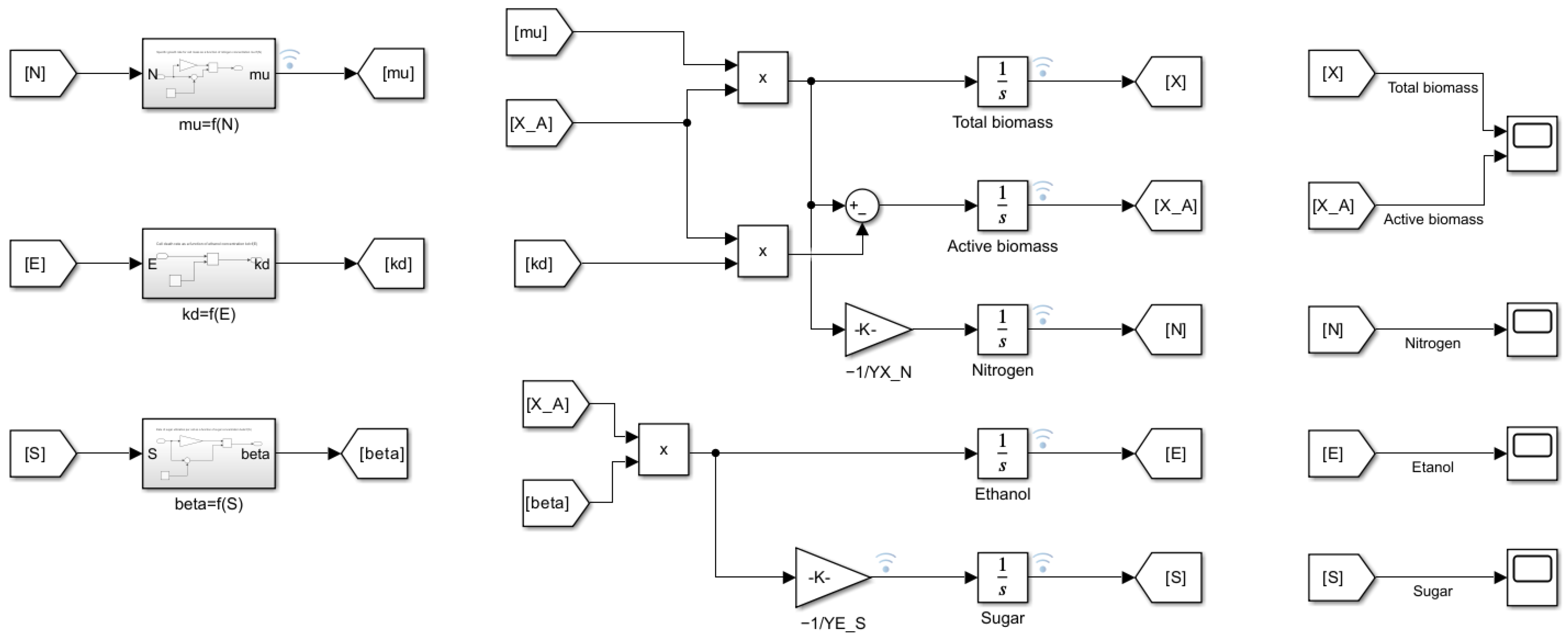
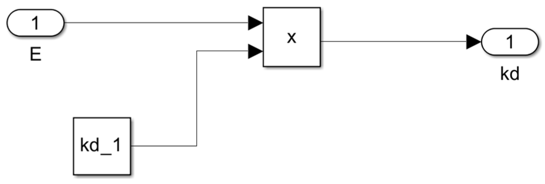
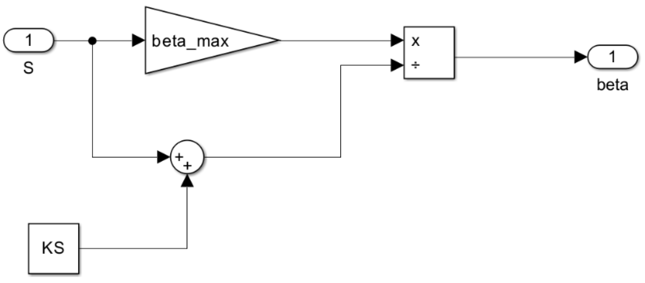
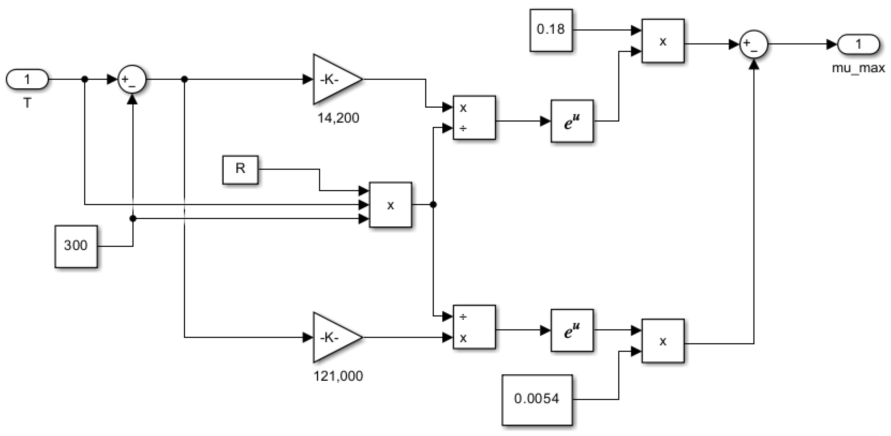
2.5.1. Coleman et al. Fermentation Model

Figure 7 presents the Simulink model, while in Figure 8, Figure 9 and Figure 10, the associated subsystems are shown.

2.5.2. Boulton Fermentation Model

Figure 11 presents the Simulink model, while in Figure 12, Figure 13, Figure 14, Figure 15, Figure 16 and Figure 17, the associated subsystems are shown.

3. Results and Discussion

Simulation results obtained using Coleman et al. model with parameter values corresponding to T = 20 °C [6]: (K_N = 10 mg·L⁻¹, μ_max = 0.06 h⁻¹, k_d’ = 0.000025 L·g⁻¹·h⁻¹, β_max = 0.2 g(S)·g(X)⁻¹·h⁻¹, K_S = 10 g·L⁻¹, Y_X/N = 25 g(X)·g(N)⁻¹, Y_E/S = 0.54 g(E)·g(S)⁻¹) and initial state variables values X(0) = 0.1 g·L⁻¹, X_A(0) = 0.1 g·L⁻¹, N(0) = 330 mg·L⁻¹, E(0) = 0 g·L⁻¹, and S(0) = 220 g·L⁻¹ are presented in Figure 18.

For simulating Boulton model, a stainless steel cylindrical tank with the following characteristics [29]: must volume in the tank V = 100 L (0.1 m³), the heat transfer area A = 1.13 m², and the overall heat transfer coefficient for natural convection U = 1.8·10³ cal·h⁻¹·m⁻²·K⁻¹ were considered. The results obtained for the initial state variables values X(0) = 0.1 g·L⁻¹, E(0) = 0 g·L⁻¹, S(0) = 220 g·L⁻¹, T(0) = 293.15 K, T_c = 293.15 K, and the parameters R = 1.987 cal·mol⁻¹·K⁻¹, Y_m= 0.1 g(X)/g(S), m₀ = 0.0002861, K_S0 = 112 g·L⁻¹, C_p = 886 cal·kg⁻¹·K⁻¹ [29], ρ = 1050 kg·m⁻³, and ΔH = 23.5·10³ cal·mol⁻¹ [29] are presented in Figure 19 and Figure 20.

The simulation results without temperature control indicate that fermentation ceases after 134 h (≈5.5 days) at an initial must temperature of 20 °C. The predicted must temperature shows a rise in temperature of 3.2 °C, with the maximum CO₂ production rate at 75.2 h after the start of the fermentation process. This time moment corresponds with the maximum fermentation rate (${\left({\displaystyle \frac{\mathrm{d}E}{\mathrm{d}t}}\right)}_{max}, {\left({\displaystyle \frac{\mathrm{d}CO2}{\mathrm{d}t}}\right)}_{max}$) and indicates the transition between the exponential growth phase and the stationary phase.

Figure 20 shows a strong correlation between the CO₂ production rate and the must temperature. In order to check if the CO₂ rate can be used for controlling the fermentation speed (responsible for aroma composition), a reference profile for the CO₂ rate, ${\left(\mathrm{d}{CO}_2/\mathrm{d}t\right)}_{ref}$, was defined (Figure 21) and used in simulations for proportional control of the external temperature, T_c:

$$T_c=k_T·\left(k_{dCO2}·\left({\left(\mathrm{d}{CO}_2/\mathrm{d}t\right)}_{ref}-\mathrm{d}{CO}_2/\mathrm{d}t\right)+{\left(\mathrm{d}{CO}_2/\mathrm{d}t\right)}_{ref}\right)$$

(9)

Figure 22 and Figure 23 indicate the results obtained by simulating Boulton’s model with T_c evolution computed using (9) with the scaling factors $k_{dCO2}=1$, $k_T=$ 5. Figure 24 and Figure 25 show the evolution of sugar concentration and ethanol concentration with and without temperature control. The simulation results indicate that the fermentation process lasts 3.3 h more when temperature control is employed.

Analysis of audio samples recorded during the fermentation process is presented in what follows. Figure 26, Figure 27 and Figure 28 show examples of audio signals recorded on the first, second, and fifth days from the beginning of the fermentation process monitoring.

The filtered RMS envelope and the extracted crossing points are illustrated in Figure 29, Figure 30 and Figure 31.

Table 2. Features extracted from the signals over different days.

Day nr.	RMS Value	Maximum Pulse Width [s]	Average Frequency [Hz]
1	0.0405	0.2175	0.6035
1	0.0512	0.7390	0.5440
2	0.0486	0.8527	0.6147
2	0.0431	0.9183	0.9235
4	0.0142	0.4318	0.5376
5	0.0202	0.5236	0.2906

indicates the features extracted from the audio signals for different days, while in Figure 32, Figure 33 and Figure 34 the graphical representations as a function of hours are presented. Figure 35 shows the graphical representation of the signal features as 3D points.

The extracted features suggest how fermentation evolves over time. An increase in values can be observed in the first two days, while in the last two days the value gradually decreased. The signals acquired in the first two days can be associated with the active or exponential growth phase, during which most of the sugar is consumed and ethanol concentration and CO₂ production increase, reflecting the yeast’s ability to metabolize sugar efficiently. In the last two days, fermentation slows significantly, with reduced RMS values, shorter pulses, and lower frequencies indicating that the signals can be associated with the quasi-stationary phase, when fermentation slows down as sugar is depleted and yeast activity diminishes. The drop in frequency by day 5 indicates reduced CO₂ bubbling, signaling that fermentation will end soon.

The frequencies in Hz corresponding to the CO₂ production rate identified from the recorded audio signals (f_exp[t_i] [Hz]) were correlated with the CO₂ rate profile obtained through simulation (CO₂Rate_sim $[\mathrm{g}·{\mathrm{L}}^{-1}·{\mathrm{h}}^{-1}]$). To accomplish this, first f_exp points were fitted by a Gaussian curve (Figure 36) with the form $f_{exp}\left(t\right)=a·e^{-{\left(\frac{t-b}{c}\right)}^2}$, a = 1.18, b = 57.21, and c = 41.23. Then, the autocorrelation was used for finding the delay between $f_{exp}\left(t\right)$ and CO₂Rate_sim (the delay value found: Δt = 41.35 h), and a scale factor was computed based on the ratio between the peak values of the two signals (s = 1/0.84). The expression obtained can be written as follows: ${CO2Rate}_{exp}\left(t\right)=s·f_{exp}\left(t-∆t\right)\approx {CO2Rate}_{sim}(t)$. Figure 37 shows the evolution of the CO₂ rate and the frequency values estimated from the audio signals. The results suggest that the first 4 points correspond to the exponential growth phase and were acquired on days 3 and 4 relative to the start of the fermentation process, while the last two points correspond to days 5 and 6 (quasi-stationary phase).

4. Conclusions

A comparative study of the most comprehensive mathematical models proposed for the wine fermentation processes was performed. Simulations performed in Matlab were used to assess these models. Among these, Coleman et al. model and Boulton model were used in simulations for analyzing the evolution of sugar concentration, ethanol concentration, must temperature, and CO₂ production rate under different initial conditions and parameters.

The CO₂ rate is the most important variable for the assessment of the fermentation process kinetics, and the main physical variable that affects this process is temperature. Estimation of CO₂ rate using acoustic-based approaches provides a non-invasive way to track fermentation stages and to make adjustments (e.g., temperature control or nutrient addition). All automated control strategies applicable to the fermentation tanks incorporating heat exchangers must rely primarily on the control of the must temperature through circulation of a warm or cold agent and stirring. Slower or faster kinetics can be prescribed through a regulatory system having as input the CO₂ rate and as output the flow rate of the heating/cooling agent through the heat exchanger.

A virtual CO₂ rate sensor was proposed, having as input the audio signal collected by a microphone and output the CO₂ rate. The digital signal processing involves acquisition, filtering, analysis, and feature extraction. The proportionality constant that relates the frequency to the CO₂ rate was identified through a numerical fitting method.

The experimental setup referred to in this paper included a small fermentation vessel (100 L). The grape must used in the experiment was obtained from pressing white grapes produced by local varieties. Further efforts will focus on validating the proposed control approach in a real fermentation plant by instrumenting a tank with a larger capacity (2000 L). This validation will be achieved by adopting the extended Boulton model and a model that accounts for the presence of aromas, as referenced in [12]. Additionally, the estimation of parameters specific to the fermentation conditions—such as maximum specific growth rate, biomass yield for nitrogen, and ethanol yield from sugar—will be based on measured datasets. More advanced control strategies, as depicted in Figure 6, will also be explored. AI (artificial intelligence) and ML (machine learning)-based techniques for correlating CO₂ and temperature profiles with aromatic compound measurements will also be considered, based on a measurement database collected with a FTIR (Fourier transform infrared spectroscopy) instrument.

References

1. Jackson, R.S. Fermentation. In Wine Science: Principles and Applications, 3rd ed.; Elsevier Inc.: Burlington, MA, USA, 2008; pp. 332–417. [Google Scholar]
2. Paar, A. Complete Your Wine Analysis. Application Report XPAIA055EN-C. Available online: https://www.anton-paar.com (accessed on 19 October 2024).
3. Mamolar-Domenech, S.; Crespo-Sariol, H.; Sáenz-Díez, J.C.; Sánchez-Roca, A.; Latorre-Biel, J.-I.; Blanco, J. A new approach for monitoring the alcoholic fermentation process based on acoustic emission analysis: A preliminary assessment. J. Food Eng. 2023, 353, 111537. [Google Scholar] [CrossRef]
4. Innocenti, R.; Ettore, P. Analysis and Experimental Validation of Mathematical Models of Wine Fermentation. Master’s Thesis, Politecnico di Milano, Milan, Italy, 2022. [Google Scholar]
5. Marsit, S.; Dequin, S. Diversity and adaptive evolution of Saccharomyces wine yeast: A review. FEMS Yeast Res. 2015, 15, fov067. [Google Scholar] [CrossRef] [PubMed]
6. Coleman, M.C.; Fish, R.; Block, D.E. Temperature-dependent kinetic model for nitrogen-limited wine fermentations. Appl. Environ. Microbiol. 2007, 73, 5875–5884. [Google Scholar] [CrossRef] [PubMed]
7. Assar, R.; Vargas, F.A.; Sherman, D.J. Reconciling Competing Models: A Case Study of Wine Fermentation Kinetics. In Algebraic and Numeric Biology; Lecture Notes in Computer Science; Horimoto, K., Nakatsui, M., Popov, N., Eds.; Springer: Berlin/Heidelberg, Germany, 2012; Volume 6479. [Google Scholar] [CrossRef]
8. Nelson, J.; Boulton, R. Models for Wine Fermentation and Their Suitability for Commercial Applications. Fermentation 2024, 10, 269. [Google Scholar] [CrossRef]
9. Liu, D.; Xu, L.; Xiong, W.; Zhang, H.T.; Lin, C.C.; Jiang, L.; Xu, B. Fermentation Process Modeling with Levenberg-Marquardt Algorithm and Runge-Kutta Method on Ethanol Production by Saccharomyces cerevisiae. Math. Probl. Eng. 2014, 2014, 289492. [Google Scholar] [CrossRef]
10. Boulton, R. The Prediction of Fermentation Behavior by a Kinetic Model. Am. J. Enol. Vitic. 1980, 31, 40–45. [Google Scholar] [CrossRef]
11. Borzi, A.; Merger, J.; Muller, J.; Rosch, A.; Schenk, C.; Schmidt, D.; Schmidt, S.; Schulz, V.; Velten, K.; von Wallbrunn, C.; et al. Novel model for wine fermentation including the yeast dying phase. arXiv 2014. Available online: https://arxiv.org/abs/1412.6068 (accessed on 15 May 2025).
12. Bartsch, J.; Borzì, A.; Schenk, C.; Schmidt, D.; Müller, J.; Schulz, V.; Velten, K. An extended model of wine fermentation including aromas and acids. arXiv 2019. Available online: https://arxiv.org/abs/1901.03659 (accessed on 15 May 2025).
13. Caro, I.; Pérez, L.; Cantero, D. Development of a Kinetic Model for the Alcoholic Fermentation of Must. Biotechnol. Bioeng. 1991, 38, 742–748. [Google Scholar] [CrossRef] [PubMed]
14. Ghadarah, N.; Ayre, D. A Review on Acoustic Emission Testing for Structural Health Monitoring of Polymer-Based Composites. Sensors 2023, 23, 6945. [Google Scholar] [CrossRef] [PubMed]
15. Barbosh, M.; Dunphy, K.; Sadhu, A. Acoustic emission-based damage localization using wavelet-assisted deep learning. J. Infrastruct. Preserv. Resil. 2022, 3, 6. [Google Scholar] [CrossRef]
16. Martini, A.; Troncossi, M.; Rivola, A. Leak Detection in Water-Filled Small-Diameter Polyethylene Pipes by Means of Acoustic Emission Measurements. Appl. Sci. 2017, 7, 2. [Google Scholar] [CrossRef]
17. Nguyen, D.-T.; Nguyen, T.-K.; Ahmad, Z.; Kim, J.-M. A Reliable Pipeline Leak Detection Method Using Acoustic Emission with Time Difference of Arrival and Kolmogorov-Smirnov Test. Sensors 2023, 23, 9296. [Google Scholar] [CrossRef] [PubMed]
18. Yang, J.; Liu, C.; Xu, Q.; Tai, J. Acoustic Emission Signal Fault Diagnosis Based on Compressed Sensing for RV Reducer. Sensors 2022, 22, 2641. [Google Scholar] [CrossRef] [PubMed]
19. Pham, M.T.; Kim, J.-M.; Kim, C.H. Intelligent Fault Diagnosis Method Using Acoustic Emission Signals for Bearings under Complex Working Conditions. Appl. Sci. 2020, 10, 7068. [Google Scholar] [CrossRef]
20. Sio-Sever, A.; Lopez, J.M.; Asensio-Rivera, C.; Vizan-Idoipe, A.; de Arcas, G. Improved Estimation of End-Milling Parameters from Acoustic Emission Signals Using a Microphone Array Assisted by AI Modelling. Sensors 2022, 22, 3807. [Google Scholar] [CrossRef] [PubMed]
21. Varner, D.; Černý, M.; Mareček, J.; Los, J. Monitoring of beer fermentation process using acoustic emission method. In Proceedings of the MendelNet, Brno, Czech Republic, 24 November 2010; pp. 651–653. Available online: https://mnet.mendelu.cz/mendelnet2010/articles/21_varner_322.pdf (accessed on 2 February 2025).
22. Oikonomou, P.; Raptis, I.; Sanopoulou, M. Monitoring and Evaluation of Alcoholic Fermentation Processes Using a Chemocapacitor Sensor Array. Sensors 2014, 14, 16258–16273. [Google Scholar] [CrossRef]
23. Lopes, T.G.; Aguiar, P.R.; França, T.V.; Conceição, P.d.O., Jr.; Soares, C., Jr.; Antonio, Z.R.F. Time-Domain Analysis of Acoustic Emission Signals during the First Layer Manufacturing in FFF Process. Eng. Proc. 2022, 27, 83. [Google Scholar] [CrossRef]
24. Hussein, W.B.; Hussein, M.A.; Becker, T. Robust spectral estimation for speed of sound with phase shift correction applied online in yeast fermentation processes. Eng. Life Sci. 2012, 12, 603–614. [Google Scholar] [CrossRef]
25. Kundu, P.; Kishore, N.K.; Sinha, A.K. Frequency domain analysis of acoustic emission signals for classification of partial discharges. In Proceedings of the 2007 Annual Report-Conference on Electrical Insulation and Dielectric Phenomena, Vancouver, BC, Canada, 14–17 October 2007; pp. 146–149. [Google Scholar] [CrossRef]
26. Press, W.H.; Teukolsky, S.A.; Vetterling, W.T.; Flannery, B.P. Numerical Recipes. In The Art of Scientific Computing, 3rd ed.; Cambridge University Press: New York, NY, USA, 2007. [Google Scholar]
27. Proakis, J.; Manolakis, D. Digital Signal Processing: Principles, Algorithms and Applications, 3rd ed.; Prentice Hall Inc.: Upper Saddle River, NJ, USA, 1996. [Google Scholar]
28. Nelson, J.; Knoesen, A.; Boulton, R. Nonlinear Model Predictive Control of Wine Fermentation Kinetics. Eng. Proc. 2023, 37, 107. [Google Scholar] [CrossRef]
29. Colombié, S.; Malherbe, S.; Sablayrolles, J.-M. Modeling of heat transfer in tanks during wine-making fermentation. Food Control 2007, 18, 953–960. [Google Scholar] [CrossRef]
Figure 1. Experimental setup for CO2 rate monitoring.
Mathematics 13 01653 g001
Figure 2. Microphone setup.
Mathematics 13 01653 g002
Figure 3. Virtual CO2 rate sensor.
Mathematics 13 01653 g003
Figure 4. Fermentation setup.
Mathematics 13 01653 g004
Figure 5. Block diagram for must temperature control.
Mathematics 13 01653 g005
Figure 6. Block diagram for nonlinear model predictive control (after [28]).
Mathematics 13 01653 g006
Figure 7. Simulink model for Coleman et al. fermentation model.
Mathematics 13 01653 g007
Figure 8. Subsystem for the specific growth rate of cells as a function of nitrogen concentration μ = f(N).
Mathematics 13 01653 g008
Figure 9. Subsystem for the cell death rate as a function of ethanol concentration kd = f(E).
Mathematics 13 01653 g009
Figure 10. Subsystem for the rate of sugar utilization per cell as a function of sugar concentration β = f(S).
Mathematics 13 01653 g010
Figure 11. Simulink model for Boulton fermentation model.
Mathematics 13 01653 g011
Figure 12. Subsystem for computing the maintenance coefficient as a function of temperature m = f(T).
Mathematics 13 01653 g012
Figure 13. Subsystem for computing the saturation constant as a function of temperature KS1 = f(T).
Mathematics 13 01653 g013
Figure 14. Subsystem for computing maximum specific growth rate as a function of temperature μmax = f(T).
Mathematics 13 01653 g014
Figure 15. Subsystem for computing the specific growth rate as a function of sugar concentration μ = f(S).
Mathematics 13 01653 g015
Figure 16. Subsystem for computing yeast viability as a function of time and ethanol concentration XV = f(t,E).
Mathematics 13 01653 g016
Figure 17. Subsystem for computing the rate of must temperature change.
Mathematics 13 01653 g017
Figure 18. Simulation results for Coleman et al. model.
Mathematics 13 01653 g018
Figure 19. Simulation results for Boulton model (without temperature control).
Mathematics 13 01653 g019
Figure 20. Must temperature vs. CO2 rate (without temperature control).
Mathematics 13 01653 g020
Figure 21. Reference CO2 rate profile ((dCO2/dt)ref) vs. CO2 rate profile without temperature control ((dCO2/dt)ntc).
Mathematics 13 01653 g021
Figure 22. Simulation results for Boulton’s model (with temperature control).
Mathematics 13 01653 g022
Figure 23. Reference CO2 rate vs. simulated CO2 rate.
Mathematics 13 01653 g023
Figure 24. Sugar concentration (without temperature control—black dotted line vs. with temperature control—blue continuous line).
Mathematics 13 01653 g024
Figure 25. Ethanol concentration (without temperature control—black dotted line vs. with temperature control—blue continuous line).
Mathematics 13 01653 g025
Figure 26. Example of recorded audio sample (day 1).
Mathematics 13 01653 g026
Figure 27. Example of recorded audio sample (day 2).
Mathematics 13 01653 g027
Figure 28. Example of recorded audio sample (day 5).
Mathematics 13 01653 g028
Figure 29. Features extracted from audio samples (day 1).
Mathematics 13 01653 g029
Figure 30. Features extracted from audio samples (day 2).
Mathematics 13 01653 g030
Figure 31. Features extracted from audio samples (day 5).
Mathematics 13 01653 g031
Figure 32. RMS value as a function of time.
Mathematics 13 01653 g032
Figure 33. Maximum value and standard deviation of the pulse widths as a function of time.
Mathematics 13 01653 g033
Figure 34. Frequency as a function of time.
Mathematics 13 01653 g034
Figure 35. Three-dimensional representation of the extracted features.
Mathematics 13 01653 g035
Figure 36. Estimated frequency modeled using a Gaussian curve.
Mathematics 13 01653 g036
Figure 37. Simulated CO2 rate vs. estimated CO2 rate.
Mathematics 13 01653 g037