Abstract
In this article, we address the problem of the parameter estimation of a partially observed linear hypoelliptic stochastic system in continuous time, a relevant problem in various fields, including mechanical and structural engineering. We propose an online approach which is an approximation to the expectation–maximization (EM) algorithm. This approach combines the Kalman–Bucy filter, to deal with partial observations, with the maximum likelihood estimator for a degenerate n-dimensional system under complete observation. The performance of the proposed approach is illustrated by means of a simulation study undertaken on a harmonic oscillator that describes the dynamic behavior of an elementary engineering structure subject to random vibrations. The unknown parameters represent the oscillator’s stiffness and damping coefficients. The simulation results indicate that, as the variance of the observation error vanishes, the proposed approach remains reasonably close to the output of the EM algorithm, with the advantage of a significant reduction in computing time.
Keywords:
EM algorithm; partially observed systems; parameter estimation; stochastic differential equations; hypoelliptic models; harmonic oscillator MSC:
62M20; 62M05; 62F12; 60H10; 60G10; 60G35; 62H12
1. Introduction
Stochastic systems play a central role in solving many practical problems in various fields, including mechanical and structural engineering, industrial control and automation, econometrics, neuroscience, computational biology, bioinformatics, and environmental monitoring, just to name a few (see, e.g., [1,2,3,4,5,6,7,8,9] and the references therein).
In mechanical and structural engineering, in particular, stochastic systems are used to model the dynamic response of structures subject to random forces, including situations where the noise captured by a component of the state affects the other state component. This scenario fits into stochastic hypoelliptic systems, which can be directly observed, such as those investigated in [1], or indirectly observed, also known as partially observed systems [3]. This is the case, for instance, when only one component of the system state is measured. An inherent challenge lies in completely identifying such systems, where the difficulty is to estimate both the state and the unknown model parameters. In the literature, one can find a diversity of studies exploring the application of partially observed stochastic systems with unknown parameters in different fields (see, for example, [3,4,8]). Some of these studies deal with the systems observed continuously in time, most of which assume a one-dimensional state and a one-dimensional observation. In this line of work, ref. [10] discusses the ergodic case, while [11,12] considered the problem of small observation noise, and [13] focuses on one-step estimators. Already in the one-dimensional case, the approach that consists in maximizing the likelihood of incomplete data generally introduces complexity into the likelihood function, making it difficult to calculate the exact gradient and obtain a closed form of the maximum likelihood estimator (MLE). As often occurs, multidimensionality brings more complexity to the problem (see, e.g., [12]). For this reason, an alternative approach widely explored in the literature is the stochastic approximation (SA) for calculating the likelihood gradient. Instead of calculating the exact gradient of the likelihood function of incomplete data, which can be computationally expensive, the SA approach uses a stochastic approximation of the likelihood function itself. Recent contributions to this modus operandi include [5,6,8,14], where parameter estimation is performed online, meaning that estimation is carried out recursively, with parameters being updated in real time from a continuous flow of observations, without the need to access previous data.
In theoretical terms, hypoelliptic systems introduce additional challenges in terms of model parameter estimation, primarily due to the non-invertibility of the diffusion covariance matrix. The parametric estimation of directly observed continuous-time stochastic differential equations (SDEs) is addressed, for example, in [1,15,16]. The analogous problem in discrete time is studied in several papers, namely [17,18,19,20] and the references therein. The complexity brought by hypoellipticity is further heightened when the system is partially observed, meaning that only some state components are accessible and are additionally observed with error. As a result, increasing difficulties in the estimation of parameters from the only observed components should be expected. The work by Iguchi et al. [21] addresses the estimation of parameters of degenerate diffusion processes with different degrees of roughness, considering full and partial multidimensional observations in discrete time. The cited article proposes estimation methods for two classes of hypoelliptic models, depending on the extent to which uncertainties are propagated into non-observed components.
To overcome the challenges associated with indirect observations, the literature proposes combining a smoothing or a filtering algorithm for the unobserved state with a maximum likelihood estimator for the directly observed problem [22]. This ends up being the idea behind the so-called estimation–maximization or simply EM algorithm, initially introduced by [23] in the time series context. The extension of the EM algorithm, as presented in [22,24], focuses on the maximum likelihood (ML) estimation of parameters for continuously partially observed processes given by SDEs. Those papers discuss the extension in detail in the framework of Markovian diffusion processes or continuous-time auto regressive moving average (CARMA) processes observed by sensors. Although the original application of the EM algorithm proposed in the time series context, the concept of a recursive EM algorithm, also known as the online EM algorithm, was subsequently explored by other authors in contexts such as hidden Markov models (HMMs) and discretely observed state space models (see, e.g., [25,26,27,28]). Picchini and Samson (2018) [29] proposed the stochastic approximation expectation–maximization with approximate Bayesian computation algorithm (SAEM-ABC) for estimating state model parameters, integrating approximate Bayesian computations with the stochastic approximation expectation–maximization algorithm (SAEM).
In what concerns the systems observed continuously in time, the comparison of the EM algorithm with the maximization of the likelihood of incomplete data for partially observed diffusion processes using offline approaches was extensively investigated in [30]. More recently, ref. [14] established a comparison between the EM algorithm and the stochastic gradient ascent (SGA) algorithm, based on the likelihood of incomplete data, targeting some online approach. In any case, it is important to note, as mentioned above, that maximizing the likelihood of incomplete data can lead to computationally demanding procedures, and different methods can show varying degrees of efficiency.
It is also worth stressing that, apart from [22,30,31], very few works address the multidimensional continuous-time problem. Indeed, a substantial part of the literature dedicated to the parameter estimation of diffusion processes focuses predominantly on one-dimensional diffusions observed in discrete time. Research related to parameter estimation of diffusion processes in the multidimensional and continuous-time case, including the properties of proposed estimators, is a considerably more untouched field.
In the present paper, we consider a 2-dimensional hypoelliptic linear SDE observed in continuous time through a one-dimensional observation process. We propose a simple approach that consists of combining the Kalman–Bucy filter (KBF) for the unobserved state with the MLE for the directly observed problem. The MLE investigated in [1,15,32] is able to address the non-regularity of the diffusion matrix that is a characteristic of hypoelliptic systems. We recall that, since the investigated system is linear, the KBF is optimal for the state estimation problem with known parameter values (see [33]). Our approach should be considered as an online approach, since it uses the estimate in the current time instant to calculate the next estimate in time, as observations become available. We propose an algorithm that approximates the EM algorithm, with the advantage that it runs considerably faster. We present the results of a simulation study which compares the performance of both algorithms as the intensity of the observation noise vanishes. The results show that the proposed algorithm stands as a computationally efficient approximation provided that the observation noise is small enough (high signal-to-noise ratio conditions).
The present paper is organized as follows: Section 2 is dedicated to the formulation of the estimation problem under study in this paper; the maximum likelihood estimation is addressed in Section 3; Section 4 and Section 5 review the KBF and the EM algorithm, respectively; Section 6 describes the proposed approximated algorithm; Section 7 reports the results of computer simulations. The paper ends with some comments on Section 8.
2. Problem Formulation
In a filtered probability space , let us consider the continuous hypoelliptic linear model described by the following 2-dimensional stochastic differential equation
representing the state of the system. Let us consider that this system is partially observed in continuous time, with equation
representing the observation process. Here, and are two independent standard 1-dimension Wiener processes, and
where represents the vector of unknown parameters. We consider that the values of and are known and is a known positive number approaching zero, i.e., . The initial condition for Equation (1), , will be considered fixed and . However, minor changes can be made in the sequel to encompass as a random variable having a known distribution.
Our problem is to estimate recursively or online based on , the -algebra of the observations until time T. We intend to study the asymptotic behavior of the MLE of as . In other words, one goal of this paper is to investigate the influence of the observation error on the estimator’s performance as the variance of the observation error approaches zero. In addition, we aim to find an approximation to the EM algorithm that provides good quality estimates of the vector of parameters .
We will denote by the 2-dimensional state vector. Remark that, in Equation (2), with H given by (3), the second-state component, , is observed through the realization of , with some error, while the first state component, , is only indirectly observed through the state dynamics.
In order to better explain the methodology, the three following sections introduce the problematic of the ML estimation of model parameters, a reminder of the Kalman–Bucy Filter and of the EM algorithm.
3. The Maximum Likelihood Estimator
The construction of the MLE for the parameter requires expressing first the likelihood function which is given by the Radon–Nikodym derivative of , the probability measure induced by , with respect to the reference measure . Then, as usual, one must maximize this function on . As seen in the estimation problems of the same type (see, e.g., [34]), computational difficulties should be expected in the optimization procedure. For this reason, we first draw some considerations on the completely observed case. That is the purpose of the next subsection (Section 3.1). The partially observed case introduced in Section 2, and which we aim to solve, is explored later in Section 3.2. In Section 3.2, additional complexity is brought up by the fact that the state is no more observed, as already addressed in the introduction. Therefore, it is not surprising that a two-step procedure may well be appropriate to capture the information on the parameter value that may be contained in the observations.
3.1. The Completely Observed Case
The case where the state is directly observed is studied in detail in [1]. Let us denote by the natural filtration of the process and recall that the observations are available. The likelihood function is given by the Radon–Nikodym derivative of with respect to the reference measure corresponding to and restricted to . It is given by the following conditional expectation:
where
as a result of applying the Girsanov theorem, with representing the Moore–Penrose inverse of .
Prior et al. [1] give us the expression of the MLE for :
which is derived from the direct maximization of as a function of . This estimator is consistent, unbiased, locally asymptotically normal, and efficient [1,15,32].
3.2. The Partially Observed Case
Recall that the construction of the MLE for the parameter requires expressing the likelihood function, but, in the partially observed case, this likelihood function depends on the conditional expectation of the unobserved state process , conditioned on the observation until time T, denoted by . Let us denote by such a conditional expectation,
As is well known, according to the innovation theorem [35], the process is also a diffusion-type process that can be rewritten as
where is a Wiener process. The Radon–Nikodym derivative of the probability measure generated by the process , given by (7), with respect to the Wiener measure, is given by
Girsanov’s theorem gives us the likelihood function
By maximizing the likelihood function L, one obtains the MLE of , here denoted :
We are interested in the asymptotic behavior of this estimator as .
4. The Kalman–Bucy Filter
The Kalman–Bucy filter (KBF) is a well-established tool for dealing with estimation problems in partially observed linear systems [33]. It can be introduced as follows.
In the context of the system (1) and (2), where is fixed and known, let us consider the problem of estimating at each time t, with , given the observations available until time t. Let us define and , which represent the conditional mean of the state process and covariance matrix, respectively, at each time t, given the available observations, that is
and
where is the -algebra generated by the observation process . In what concerns linear SDEs with the Gaussian initial condition, computing (11) and (12), at each time t, is equivalent to computing the conditional distribution of given , since this conditional distribution would be Gaussian as well. Now, this conditional distribution is the optimal solution to the state estimation problem in terms of the mean square error. It happens that computing (11) and (12), at each time t, can be performed by solving the so-called KBF equations (see, e.g., [36]):
The Kalman gain, , is given by
and the initial conditions and are used. Equation (14) is commonly known as the Riccati equation.
5. The EM Algorithm
The EM algorithm is an iterative method designed to maximize the likelihood function, previously here denoted by L. Its application is particularly useful in situations involving partially observed systems, where observations may contain noise or involve only part of the state components. Under the conditions specified in Section 2 for the system (1) and (2), let denote the probability measure induced by and . Let us recall that our goal is to estimate based on the available observations, that is on .
As stated in [22], we assume that, for any and in the parameter space , the probability measures and are mutually absolutely continuous. This implies that , with , forms a family of mutually absolutely continuous probability measures and therefore ensures the existence of the Radon–Nikodym derivative of with respect to . Additionally, we assume that, for any and in , with , one has
This condition is known as the identifiability assumption, and it ensures that and are distinguishable given .
According to Girsanov’s theorem, the log-likelihood function is given by the following conditional expectation
where is the Radon–Nikodym derivative of with respect to the reference measure corresponding to and restricted to . As usual, represents the expectation under measure .
In each iteration of the EM algorithm, two steps are involved, namely the expectation step (E-step) and the maximization step (M-step). The algorithm can be described as follows:
Step 1. Begin with and choose the initial guess .
Step 2 (E-step). Set as the estimate after the n-th iteration and compute the function
Step 3 (M-step). Determine
Step 4. Update n to and repeat the process starting from Step 2 until a predefined stopping criterion is met.
The resulting sequence yields non-decreasing values of the log-likelihood function. This is a result of Jensen’s inequality, since
It implies that, for each value of , the log-likelihood function is globally bounded from below:
Concerning the sufficient conditions for convergence, we know from the literature that the EM algorithm finds a local maximum or a stationary value of the likelihood function and that the sequences of parameter estimates provided by the EM algorithm converge to a local maximum of the likelihood function [37]. However, convergence may be slow [30].
Next, let us concentrate on the application of the EM algorithm in the special case of the hypoelliptic system (1) and (2). The application closely follows the method described by [22], combined with the parameter estimator expression first obtained by [15], and later extended in [1,32]. We now explain how to compute the function Q.
First notice that, when updating the estimates from to , we obtain from (17) that the log-likelihood function can be written as follows:
Using (3) and performing the necessary algebraic manipulations on (20), we can write:
with representing the diffusion coefficient of (see Equations (1) and also (3)).
To obtain , defined by (18), one can resort to the smoothed estimates of the quantities
These smoothed estimates can be calculated using Kalman smoothing (see [22]). The function can be written as
for some that does not depend on . Therefore, the maximization computed in [1] can be used here. This means that the M-step in the th iteration of the EM algorithm gives
What we described above is the basis of the EM algorithm, as introduced by Dembo and Zeitouni [22]. It should be noted that, in models with high-dimensional data and in real time, this algorithm can become inconvenient due to its high computational cost, requiring storage and several passes through the dataset. Versions of Dembo and Zeitouni’s algorithm have been later developed where it is possible to estimate the parameters related to unobserved states without storing data, allowing the dataset to be processed only once (see [38,39,40,41]). These other versions are named online EM algorithms. The main underlying idea is that the current parameter estimate is used to calculate the next estimate. The expectation step is replaced by some stochastic approximation, while the previously described maximization step remains unchanged. That is what we propose in the next section (Section 6).
6. An Approximation to the EM Algorithm
We recall the framework of the problem that we intend to solve. In system (1) and (2), the state is only partially observed. The component is observed with added noise, through the realization of , with t running from 0 to T, while is not observed. Our goal is to estimate the vector of parameters recursively, or online, based on the available information at each time instant t. An estimator for the drift matrix for two-dimensional degenerate systems with complete observation was presented in Section 3.1, Equation (6). This estimator maximizes the likelihood function given , at each time t. However, in the framework of system (1) and (2), the likelihood function cannot be determined as in Section 3.1 due to the indirect character of the observations with respect to the state. On the other hand, as already mentioned, a simple procedure to simultaneously estimate both the states and the parameters of the system by maximizing the likelihood function is found not feasible [30]. Difficulties can be overcome if one thinks of the state as being estimated before maximizing the likelihood function.
Below, we describe an online algorithm for approximately estimating both the state and the parameters of the system (1) and (2) which combines the KBF of the system assuming that parameters are known with the MLE of the system assuming that the system state is known. The KBF is used to estimate and update the unobserved state, handling the indirect observations of the system, while the MLE is used to estimate the parameters based on the estimated states, all addressing the singularity of the diffusion matrix.
Step 1 (Initialization). Initialize time with . Set the guess conditions, , for the parameter vector.
Step 2 (KBF). At time t, given the observation path and the parameter , use the KBF to estimate .
Step 3 (Parameter update). Use the MLE to update to a new value , using
Keep iterating (Step 2 + Step 3) until . Terminate.
7. Simulation Study
We consider the system given by (1) and (2) with , and . The initial state is and the maximum run time is . The choice of the parameters that appear in the state Equation (1) is such that the results reported in this paper can also be discussed by comparing to the results obtained in [1], for the completely observed case, when the observation noise intensity is close to zero. Obviously, since we now observe only the state component , we should expect the parameters’ estimation error to be larger than that found in [1] and getting closer to the results there obtained as . We consider and analyze the bias and the root mean square error of the estimates (RMSE) as .
The results obtained on the numerical simulation performed on 200 generated trajectories with the time step equal to are presented in the sequel (Figure 1, Figure 2, Figure 3, Figure 4, Figure 5, Figure 6 and Table 1, Table 2, Table 3). We apply the proposed approximated online EM algorithm to the simulated observation trajectories. The vector is used as an initial guess for when the algorithm starts.
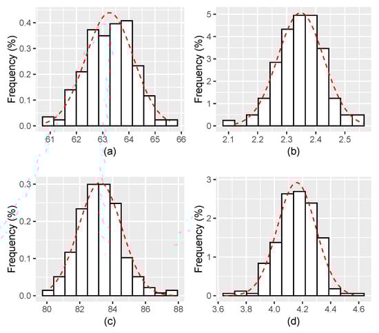
Figure 1.
Histograms for the estimates of and with . (a,b) The estimates of, respectively, and for ; and (c,d) The estimates of, respectively, and for .
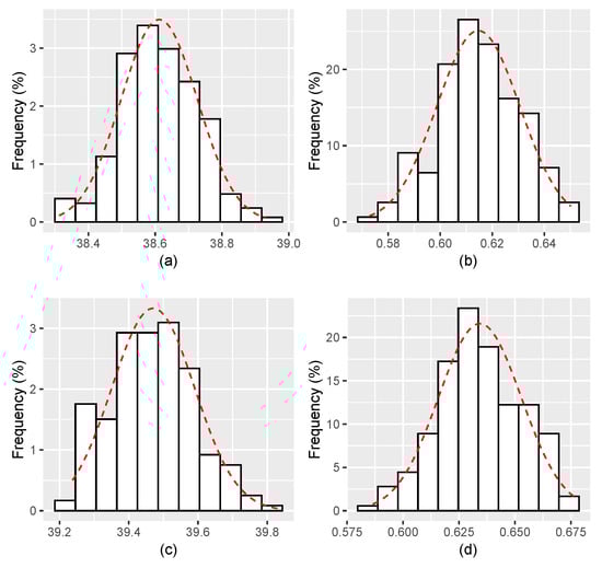
Figure 2.
Histograms for the estimates of and with . (a,b) The estimates of, respectively, and for ; and (c,d) The estimates of, respectively, and for .
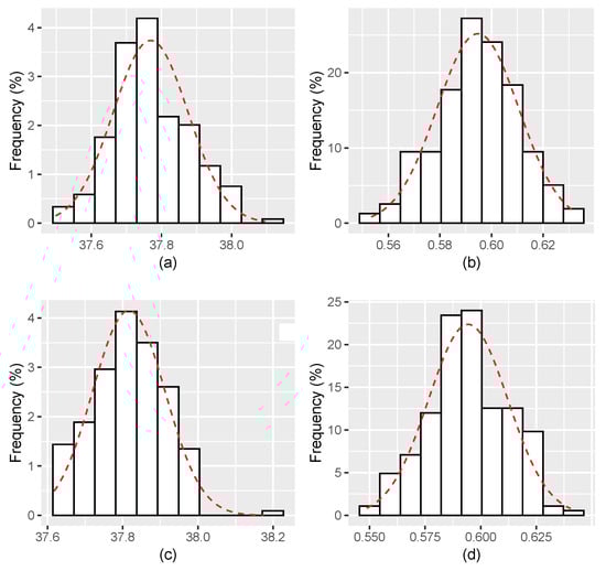
Figure 3.
Histograms for the estimates of and with . (a,b) The estimates of, respectively, and for ; and (c,d) The estimates of, respectively, and for .
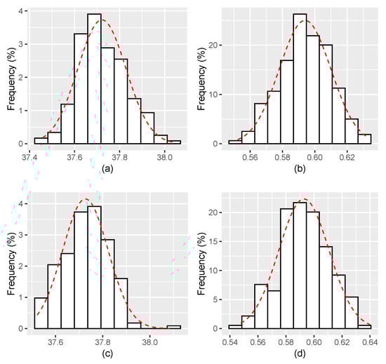
Figure 4.
Histograms for the estimates of and with . (a,b) The estimates of, respectively, and for ; and (c,d) The estimates of, respectively, and for .
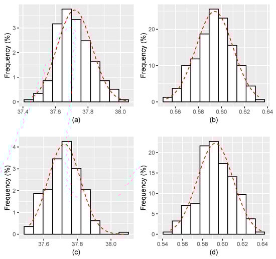
Figure 5.
Histograms for the estimates of and with . (a,b) The estimates of, respectively, and for ; and (c,d) show the estimates of, respectively, and for .
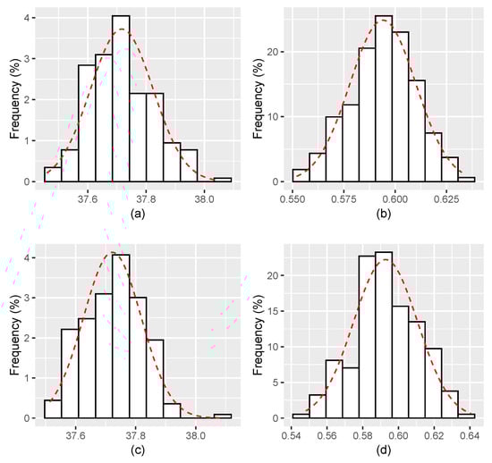
Figure 6.
Histograms for the estimates of and with . (a,b) The estimates of, respectively, and for ; and (c,d) The estimates of, respectively, and for .

Table 1.
The results of the Shapiro–Wilk normality test applied to the estimates obtained for and , at and different values of .
Table 2.
Results of the Lilliefors version of the Kolmogorov–Smirnov test applied to the estimates obtained for and , with and different values of .
Table 3.
Bias and RMSE for and different values of .
From a computational point of view, following a standard approach in simulation studies, the discretization of the integrals that appear in (6) is used as given below in the expressions (23) to (27):
Figure 1, Figure 2, Figure 3, Figure 4, Figure 5, Figure 6 display the histograms of the obtained parameter estimates for both and , with decreasing values of the signal-to-noise ratio (). On top of each figure, the histograms are drawn for , and for at the bottom of the figure. In all scenarios, the red dashed line represents the fitted Gaussian curve.
The results for (Figure 1) suggest that the parameters estimates are very far from their true values and are also very different for the different values of T. The reason for this may be that the estimating procedure did not converge yet and thus the algorithm is unable to properly estimate the parameters. One would expect the quality of the estimates to increase as the observation noise vanishes, at least for large values of T.
The results obtained for a smaller value of , more precisely , depicted in Figure 2, show estimates apparently getting closer to the true values of the parameters, but the estimation error is still large. Also, a large bias is yet observed in the simulations.
The results of applying the proposed estimation algorithm look more reasonable when the considered values of the noise intensity are smaller, going from (see Figure 3 and on Figure 4, Figure 5 and Figure 6). The estimates get closer to the true parameter values as vanishes, bias decreases, and the Gaussian curve fits the histogram better and better.
Table 1 and Table 2 show, respectively, the results of applying the Shapiro–Wilk normality test and the Lilliefors version of the Kolmogorov–Smirnov test to the samples constituted by the estimates of and . For each value of , both the p-values and the test statistics are provided. The results of the Shapiro–Wilk test indicate that the estimates for do not follow a normal distribution (), except for and . In contrast, the estimates for show no significant deviation from normality. Concerning the Lilliefors version of the Kolmogorov–Smirnov test, there is no strong evidence to reject the hypothesis that the estimates of and follow a normal distribution. Although the Shapiro–Wilk test is widely recognized for its statistical power in assessing normality, its application is generally recommended to sample sizes of up to . It is a fact that, in larger samples, this test can detect even trivial deviations from the null hypothesis. Therefore, for this analysis, the results of the Lilliefors version of the Kolmogorov–Smirnov test are more appropriate.
Table 3 summarizes the results obtained for the estimated bias and RMSE regarding parameters and , as . A fast decrease with is observed in both the bias and the RMSE, indicating that, as expected, as the measurement error decreases, the estimates become more accurate and less biased. However, after an initial fast decrease, bias and RMSE both appear to stabilize, suggesting that further reduction in the estimation errors may not result in substantial improvements in the estimates of and . One should recall that greater variability in parameter estimates is expected in this problem when compared to the completely observed system due to the indirectly observed nature of the state. This is supported by the much higher relative variation found in the estimates of and as .
In brief, the apparent improvement of the estimation procedure as vanishes, seen in Figure 1, Figure 2, Figure 3, Figure 4, Figure 5 and Figure 6, is corroborated by the results of the goodness of fit Lilliefors test (Table 2). The results obtained in the computation of the sample bias and of the RMSE go in the same direction (Table 3).
It is also important to compare the proposed approximated algorithm with the EM algorithm. Figure 7 shows the results of the comparison between the two. It can be seen that, for small values of , the proposed algorithm is reasonably close to the EM algorithm, with a significant reduction in computational complexity. As a matter of fact, the computation time has been reduced to approximately one-third of the time required for the EM algorithm. Although both algorithms exhibited some bias, the proposed algorithm showed a slightly higher bias, around higher in and in . However, one should not consider this disturbing compared to the values of the RMSE.
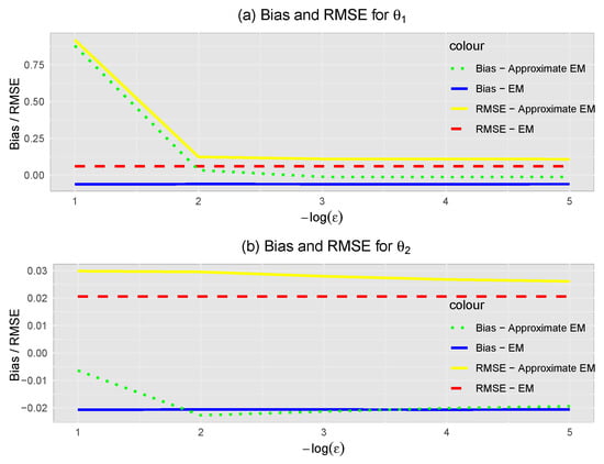
Figure 7.
Bias and RMSE for parameters and .
The RMSE of the proposed algorithm, although higher than that of the EM algorithm, apparently converges to similar values, eventually more slowly.
Note that a direct comparison of the bias and RMSE values between and is not possible, since these parameters play different roles in the model equations and, in practical problems, are even defined in different units of magnitude.
8. Conclusions and Final Comments
The present study contributes to the problem of parameter estimation in partially observed hypoelliptic linear stochastic systems. We adapted the maximum likelihood estimator (MLE) for 2-dimensional degenerate systems under complete observation, combining it with the Kalman–Bucy filter (KBF) to draw an approximate estimation algorithm. Emphasis was given to the asymptotic behavior of the estimates as the observation error tends towards zero.
The results of the simulations indicated that the performance of the proposed algorithm can significantly depend on the size of the time window in which the observations are made. Moreover, as expected, the algorithm’s performance demonstrated to be mostly sensitive to the magnitude of the system’s observation error. A substantial reduction in the observation error magnitude meant that the parameter estimates converged to their true values, with a significant reduction in bias and root mean square error. In other words, for not too large, the proposed algorithm was reasonably close to the EM, and with a substantial reduction in computational cost. The results obtained are relevant because they show that it is possible to overcome the challenges of indirect observation and the singularity of the diffusion matrix, and obtain reliable estimates of the system’s parameters. In practical applications, the proposed approach offers an effective tool for estimating parameters in areas such as mechanical and structural engineering. In addition, the methodology followed can serve as a basis for the development of new estimation techniques in more complex scenarios.
Given that the present study was focused on a two-dimensional linear model, generalization to higher-dimensional nonlinear models may present additional challenges. An approach based on the averaging principle (see, e.g., [42,43]) may help to find suitable approximate solutions and avoid system complexity. The asymptotic analysis performed with observation error intensity converging to zero may not fully reflect the estimator’s performance in practical scenarios with a finite signal-to-noise ratio. Future work should explore the application of the proposed algorithms to higher-dimensional nonlinear models, evaluate their performance in scenarios with a larger observation error, and investigate the incorporation of other techniques, such as Bayesian computing, data science methods, and artificial intelligence.
Author Contributions
Conceptualization and methodology, P.M.-O.; software, N.O.B.Á.; formal Analysis, P.M.-O. and N.O.B.Á.; supervision, P.M.-O.; visualization, P.M.-O. and N.O.B.Á.; writing, P.M.-O. and N.O.B.Á. All authors have read and agreed to the published version of the manuscript.
Funding
The work was partially supported by CMUP, a member of LASI, which is financed by national funds through FCT—Fundação para a Ciência e a Tecnologia, I.P., under the projects UIDB/00144/2020 and UIDP/00144/2020, and by INAGBE (National Institute for Scholarship Management), an institution belonging to the Ministry of Higher Education, Science, Technology and Innovation of the Government of Angola.
Data Availability Statement
The original contributions presented in this study are included in the article. Further inquiries can be directed to the corresponding author.
Conflicts of Interest
The authors declare no conflicts of interest.
Notation and Abbreviations
The following notations and abbreviations are used in this manuscript:
| * | represents the transpose (of a matrix) |
| ABC | approximate Bayesian computation |
| CARMA | continuous-time auto regressive moving average |
| E-Step | expectation step |
| EM | expectation–maximization |
| HMMs | hidden Markov models |
| KBF | Kalman–Bucy filter |
| M-Step | maximization step |
| MLE | maximum likelihood estimator |
| RMSE | root mean square error |
| SA | stochastic approximation |
| SAEM | stochastic approximation expectation–maximization |
| SDE | stochastic differential equation |
| SGA | stochastic gradient ascent |
References
- Prior, A.; Kleptsyna, M.; Milheiro-Oliveira, P. On Maximum Likelihood Estimation of the Drift Matrix of a Degenerated O–U Process. Stat. Inference Stoch. Process. 2017, 20, 57–78. [Google Scholar] [CrossRef][Green Version]
- Chen, F.; Agüero, J.C.; Gilson, M.; Garnier, H.; Liu, T. EM-based identification of continuous-time ARMA Models from irregularly sampled data. Automatica 2017, 77, 293–301. [Google Scholar] [CrossRef]
- Clairon, Q.; Samson, A. Optimal control for estimation in partially observed elliptic and hypoelliptic linear stochastic differential equations. Stat. Inference Stoch. Process. 2022, 23, 105–127. [Google Scholar] [CrossRef]
- Pokern, Y.; Stuart, A.M.; Wiberg, P. Parameter Estimation for Partially Observed Hypoelliptic Diffusions. J. R. Statist. Soc. B 2009, 71, 49–73. [Google Scholar] [CrossRef]
- Sharrock, L.; Kantas, N. Joint Online Parameter Estimation and Optimal Sensor Placement for the Partially Observed Stochastic Advection-Diffusion Equation. SIAM-ASA J. Uncertain. Quantif. 2022, 10, 55–95. [Google Scholar] [CrossRef]
- Sharrock, L.; Kantas, N.; Parpas, P.; Pavliotis, G.A. Online Parameter Estimation for the McKean–Vlasov Stochastic Differential Equation. Stoch. Process. Their Appl. 2023, 162, 481–546. [Google Scholar] [CrossRef]
- Liu, Z.; Zhao, S.; Luan, X.; Liu, F. Online state and inputs identification for stochastic systems using recursive expectation-maximization algorithm. Chemom. Intell. Lab. Syst. 2021, 217, 104403. [Google Scholar] [CrossRef]
- Sharrock, L.; Kantas, N. Two-timescale Stochastic Gradient Descent in Continuous Time With Applications to Joint Online Parameter Estimation and Optimal Sensor Placement. Bernoulli 2023, 29, 1137–1165. [Google Scholar] [CrossRef]
- Wang, Z.; Sirignano, J. Continuous-time stochastic gradient descent for optimizing over the stationary distribution of stochastic differential equations. Math. Financ. 2023, 34, 348–424. [Google Scholar] [CrossRef]
- Kutoyants, Y.A. Statistical Inference for Ergodie Diffusion Processes; Springer: Berlin/Heidelberg, Germany, 2004. [Google Scholar]
- Kutoyants, Y.A. Identification of Dynamical Systems with Small Noise; Springer: Berlin/Heidelberg, Germany, 1994. [Google Scholar]
- Kutoyants, Y.A. On parameter estimation of the hidden Ornstein–Uhlenbeck process. J. Multivar. Anal. 2019, 169, 248–263. [Google Scholar] [CrossRef]
- Kutoyants, Y.A. On parameter estimation of hidden ergodic Ornstein-Uhlenbeck process. Electron. J. Stat. 2019, 13, 4508–4526. [Google Scholar] [CrossRef]
- Surace, S.C.; Pfister, J.P. Online maximum-likelihood estimation of the parameters of partially observed diffusion processes. IEEE Trans. Autom. Control. 2019, 64, 2814–2829. [Google Scholar] [CrossRef]
- Koncz, K. On the Parameter Estimation of Diffusional Type Processes with Constant Coefficients. Anal. Math. 1987, 13, 75. [Google Scholar] [CrossRef]
- Brockwell, P.J.; Davis, R.A.; Yang, Y. Continuous-Time Gaussian Autoregression. Stat. Sin. 2007, 17, 63–80. [Google Scholar]
- Sørensen, H. Estimation of diffusion parameters for discretely observed diffusion processes. Bernoulli 2002, 8, 491–508. [Google Scholar]
- Shimizu, Y.; Yoshida, N. Estimation of Parameters for Diffusion Processes with Jumps from Discrete Observations. Stat. Inference Stoch. Process. 2006, 9, 227–277. [Google Scholar] [CrossRef]
- Yoshida, N. Estimation for Diffusion ProcessesFfrom Discrete Observation. J. Multivar. Anal. 1992, 41, 220–242. [Google Scholar] [CrossRef]
- Kurisaki, M. Parameter estimation for ergodic linear SDEs from partial and discrete observations. Stat. Inference Stoch. Process. 2023, 26, 279–330. [Google Scholar] [CrossRef]
- Iguchi, Y.; Beskos, A.; Graham, M.M. Parameter inference for degenerate diffusion processes. Stoch. Process. Their Appl. 2024, 174, 104384. [Google Scholar] [CrossRef]
- Dembo, A.; Zeitouni, O. Parameter Estimation of Partially Observed Continuous Time Stochastic Processes via the EM Algorithm. Stoch. Process. Their Appl. 1986, 23, 91–113. [Google Scholar] [CrossRef]
- Dempster, A.P.; Laird, N.M.; Rubin, D.B. Maximum Likelihood from Incomplete Data via the EM Algorithm. J. R. Stat. Soc. Ser. (Methodol.) 1977, 39, 1–38. [Google Scholar] [CrossRef]
- Dembo, A.; Zeitouni, O. Parameter Estimation of Partially observed Continuous Time Stochastic Processes via the EM Algorithm. Stoch. Process. Their Appl. 1992, 40, 359–361. [Google Scholar] [CrossRef]
- Krishnamurthy, V.; Moore, J. On-line estimation of hidden Markov model parameters based on the Kullback–Leibler information measure. IEEE Trans. Signal Process. 1993, 41, 2557–2573. [Google Scholar] [CrossRef]
- Mongillo, G.; Deneve, S. Online learning with hidden Markov models. Neural Comput. 2008, 20, 1706–1716. [Google Scholar] [CrossRef] [PubMed]
- Cappe, O. Online sequential Monte Carlo EM algorithm. In Proceedings of the 2009 IEEE/SP 15th Workshop on Statistical Signal Processing, Cardiff, UK, 31 August–3 September 2009; pp. 37–40. [Google Scholar] [CrossRef]
- Cappé, O. Online EM algorithm for hidden Markov models. J. Comput. Graph. Stat. 2011, 20, 728–749. [Google Scholar] [CrossRef]
- Picchini, U.; Samson, A. Coupling stochastic EM and approximate Bayesian computation for parameter inference in state-space models. Comput. Stat. 2018, 33, 179–212. [Google Scholar] [CrossRef]
- Campillo, F.; Gland, F. MLE for partially observed diffusions: Direct maximization vs. the em algorithm. Stoch. Process. Their Appl. 1989, 33, 245–274. [Google Scholar] [CrossRef]
- Elliott, R.; Krishnamurthy, V. Finite dimensional filters for maximum likelihood estimation of continuous-time linear Gaussian systems. In Proceedings of the 36th IEEE Conference on Decision and Control, San Diego, CA, USA, 10–12 December 1997; Volume 5, pp. 4469–4474. [Google Scholar] [CrossRef]
- Lin, N.; Lototsky, S.V. Second-order continuous-time non-stationary Gaussian autoregression. Stat. Inference Stoch. Process. 2014, 17, 19–49. [Google Scholar] [CrossRef]
- Kalman, R. A New Approach to Linear Filtering and Predictions Problems. Asme J. Basic Eng. 1960, 82, 35–45. [Google Scholar] [CrossRef]
- Kutoyants, Y.A. Hidden Ergodic Ornstein-Uhlenbeck Process and Adaptive Filter. arXiv 2023, arXiv:2304.08857. [Google Scholar] [CrossRef]
- Lipttser, R.; Shiryaev, A. Statistics of Random Processes I; Springer: New York, NY, USA, 2001; Volume I. [Google Scholar]
- Jazwinski, A. Stochastic Processes and Filtering Theory; Academic Press Inc.: Cambridge, MA, USA, 1970; Volume 64, pp. 1–371. [Google Scholar]
- Wu, C.F.J. On the Convergence Properties of the EM Algorithm. Ann. Stat. 1983, 11, 95–103. [Google Scholar] [CrossRef]
- Titterington, D.M. Recursive Parameter Estimation Using Incomplete Data. J. R. Stat. Soc. Ser. (Methodol.) 1984, 46, 257–267. [Google Scholar] [CrossRef]
- Lange, K. A Gradient Algorithm Locally Equivalent to the Em Algorithm. J. R. Stat. Soc. Ser. (Methodol.) 1995, 57, 425–437. [Google Scholar] [CrossRef]
- Cappé, O.; Moulines, E. On-Line Expectation–Maximization Algorithm for latent Data Models. J. R. Stat. Soc. Ser. Stat. Methodol. 2009, 71, 593–613. [Google Scholar] [CrossRef]
- Nguyen, H.D.; Forbes, F.; Fort, G.; Cappé, O. An Online Minorization-Maximization Algorithm. In Conference of the International Federation of Classification Societies; Studies in Classification, Data Analysis, and Knowledge Organization; Springer: Cham, Switzerland, 2023; pp. 263–271. [Google Scholar] [CrossRef]
- Khasminskij, R.Z. On the principle of averaging the Itov’s stochastic differential equations. Kybernetika 1968, 4, 260–279. [Google Scholar]
- Zou, J.; Luo, D. A new result on averaging principle for Caputo-type fractional delay stochastic differential equations with Brownian motion. Appl. Anal. 2024, 103, 1397–1417. [Google Scholar] [CrossRef]


Disclaimer/Publisher’s Note: The statements, opinions and data contained in all publications are solely those of the individual author(s) and contributor(s) and not of MDPI and/or the editor(s). MDPI and/or the editor(s) disclaim responsibility for any injury to people or property resulting from any ideas, methods, instructions or products referred to in the content. |
© 2025 by the authors. Licensee MDPI, Basel, Switzerland. This article is an open access article distributed under the terms and conditions of the Creative Commons Attribution (CC BY) license (https://creativecommons.org/licenses/by/4.0/).