Abstract
This paper presents N-bipolar soft expert (N-BSE) sets, a novel framework designed to enhance multi-attribute group decision-making (MAGDM) by incorporating expert input, bipolarity, and non-binary evaluations. Existing MAGDM approaches often lack the ability to simultaneously integrate positive and negative assessments, especially in nuanced, multi-valued evaluation spaces. The proposed N-BSE model addresses this limitation by offering a comprehensive, mathematically rigorous structure for decision-making (DM). Fundamental operations of the N-BSE model are defined and analyzed, ensuring its theoretical consistency and applicability. To demonstrate its practical utility, the N-BSE model is applied to a general case study on sustainable energy solutions, illustrating its effectiveness in handling complex DM scenarios. An algorithm is proposed to streamline the DM process, enabling systematic and transparent identification of optimal alternatives. Additionally, a comparative analysis emphasizes the advantages of the N-BSE model over existing MAGDM frameworks, highlighting its capacity to integrate diverse expert opinions, evaluate both positive and negative attributes, and support multi-valued assessments. By bridging the gap between theoretical development and practical application, this paper contributes to advancing DM methodologies.
Keywords:
N-bipolar soft expert sets; N-bipolar soft sets; N-soft sets; soft expert sets; decision making; environmental sustainability; MAGDM MSC:
03E72; 03E75; 90B50
1. Introduction
In 1965, Zadeh [1] introduced fuzzy set theory, revolutionizing mathematics by allowing partial membership to better represent imprecise human knowledge, which quickly spread to various fields. This concept was later generalized in numerous successful ways, including L-fuzzy sets [2], type-2 fuzzy sets [3], intuitionistic fuzzy sets [4], rough fuzzy sets and fuzzy rough sets [5], bipolar fuzzy sets [6], complex fuzzy sets [7], hesitant fuzzy sets [8], Pythagorean fuzzy sets [9], picture fuzzy sets [10], spherical fuzzy sets [11], Fermatean fuzzy sets [12], neutrosophic fuzzy sets [13], q-rung orthopair fuzzy sets [14], and others. Pawlak [15] introduced rough set theory in 1982, utilizing an equivalence relation called the indiscernibility relation to define lower and upper approximations and the boundary region of a set. The lower approximation includes elements definitely belonging to a concept, while the upper approximation contains elements that may belong. The difference between these approximations is the boundary region, which is empty for crisp sets and non-empty for rough sets. Rough set theory offers the advantage of extracting useful information without requiring extra parameters or information about the data. In 1994, Pawlak [16] proposed a unified approach that combined classical set theory, rough sets, and fuzzy sets to represent soft sets (S-sets). This approach inspired Molodtsov [17] to create S-set theory in 1999, where he explored its basic principles, applications, and future directions. S-set theory, which is especially useful in handling imprecise data, has shown promise in resolving ambiguities in data mining problems. Furthermore, S-set theory can expand and enhance existing concepts such as probability, fuzzy sets, rough sets, and intuitionistic fuzzy sets, addressing the lack of parameterization tools in these areas. Since its introduction, numerous authors have proposed extensions, hybridizations, and generalizations of S-set theory.
The fundamental operations associated with S-sets and their properties were initially presented in [18], and subsequently refined in [19]. Notable contributors to this field, such as [20,21], demonstrated how Molodtsov’s concept could be integrated with other well-established theories, including fuzzy sets and intuitionistic fuzzy sets. These connections between models continued to be explored [22,23]. Over time, various extensions and hybrid models emerged, including generalized intuitionistic fuzzy S-sets [24], Fermatean vague soft sets [25], bipolar soft (BS) sets [26], fuzzy BS sets [27], bipolar complex fuzzy soft sets [28], probabilistic and dual probabilistic S-sets [29,30], N-soft (N-S) sets [31], N-bipolar soft (N-BS) sets [32], N-hypersoft sets [33], bipolar hypersoft sets [34,35,36,37], M-parametrized N-S sets [38], bipolar M-parametrized N-S sets [39], hesitant fuzzy S-sets [40], m-polar fuzzy S-sets [41], ranked S-sets [42], soft rough sets, and rough S-sets [43,44]. A comprehensive literature review of S-set theory was conducted in [45]. A key area of research pertains to DM, with foundational work credited to [46,47], while [48] introduced DM within the hybrid fuzzy S-set framework, later enhanced in [49,50]. DM in generalized intuitionistic fuzzy S-sets appeared in [24]. A recent perspective on these topics can be found in [51,52].
It is worth noting that, over time, S-set theory and its hybrid models have been effectively applied in group DM, particularly in fields such as medicine, physics, and social sciences, where uncertain data often arises. One challenge faced by practitioners using questionnaires is that these mathematical techniques typically process data from only a single expert’s assessment, limiting their ability to incorporate multiple perspectives. To address this, the concept of soft expert (SE) sets was introduced by Alkhazaleh and Salleh [53], allowing for the full inclusion of each selected expert’s opinion in DM problems. The concept was later extended by [54] through the integration of fuzzy sets. Further developments in SE sets have led to the incorporation of various models aimed at DM under uncertainty, including intuitionistic fuzzy SE sets [55], N-soft expert (N-SE) sets and fuzzy N-SE sets [56], generalized neutrosophic SE sets [57], and bipolar soft expert (BSE) sets [58,59]. Convexity-cum-concavity on fuzzy SE sets [60], complex neutrosophic SE sets [61], and the use of Pythagorean fuzzy N-SE knowledge in group DM [62] have broadened the scope of the theory. Other models, such as spherical fuzzy N-SE sets [63], bipolar N-SE sets [64], and possibility neutrosophic SE sets [65], showcase the flexibility of these models in multi-criteria DM. Additional applications of these methods can be found in fields like recruitment [66] and election prediction [67]. Another perspective on the SE set and its application in multi-criteria decision-making is discussed in [68].
1.1. Motivations, Objectives, and Contributions
The motivation behind this paper stems from the limitations of existing MAGDM models in handling nuanced evaluations and expert opinions. Current approaches often fall short in incorporating both positive and negative assessments simultaneously, particularly in multi-valued evaluation spaces. The need for a comprehensive framework that balances expert input, bipolarity, and non-binary evaluations is evident in various real-world scenarios, such as sustainability assessments, healthcare prioritizations, and engineering project evaluations. This gap inspired the development of the N-BSE model, which aims to address these shortcomings by offering a robust and versatile DM framework.
The primary objectives of this paper are as follows:
- Proposing a novel N-BSE model that extends traditional SE set frameworks by integrating bipolarity and multinary evaluations.
- Defining and analyzing the core operations of the N-BSE model, ensuring its mathematical consistency and applicability.
- Demonstrating the practical utility of the N-BSE model in solving complex MAGDM problems, particularly those requiring nuanced assessments and expert collaboration.
- Conducting a comparative analysis between the N-BSE model and existing frameworks, highlighting its advantages and addressing its limitations.
This paper makes the following key contributions to the field of DM:
- Introducing the N-BSE model, a hybrid set-theoretic framework that combines expert input, bipolarity, and non-binary evaluations, addressing a significant gap in MAGDM methodologies.
- Providing rigorous definitions and fundamental operations for the N-BSE model, establishing its theoretical underpinnings.
- Proposing a systematic algorithm for applying the N-BSE model to MAGDM scenarios, enabling objective and transparent DM processes.
- Demonstrating the applicability of the N-BSE model through a detailed case study on sustainable energy solutions, illustrating its potential for real-world DM.
- Offering a comprehensive comparison with existing MAGDM models, showcasing the N-BSE model’s ability to integrate expert opinions, handle bipolarity, and support multi-valued assessments effectively.
By addressing both theoretical and practical aspects, this paper establishes the groundwork for further research and application of the N-BSE model in various domains, contributing to the progress of DM frameworks.
1.2. Outline of the Paper
This paper is organized as follows: Section 2 reviews the foundational concepts related to S-sets, SE sets, BS sets, BSE sets, N-S sets, N-SE sets, and N-BS sets, which provide the theoretical background for the study. Section 3 presents the novel N-BSE model, defines its core operations, and discusses its algebraic properties, illustrated with examples. In Section 4, the application of the N-BSE model to MAGDM is explored, including a general case study on selecting sustainable energy solutions. Section 5 provides a comparative analysis of the N-BSE model, highlighting its advantages, comparing it to existing models, and discussing its limitations. Finally, Section 6 concludes the paper and outlines potential directions for future research.
2. Preliminary Concepts
This section reviews the key concepts of S-set, SE set, BS set, BSE set, N-S set, N-SE set, and N-BS set, which serve as the foundation for this study. In this context, represents the universal set of alternatives (or objects), stands for a set of attributes (or parameters), and where refers to a set of ordered grades. The set denotes a set of experts, and corresponds to a set of opinions. Furthermore, ¥ and ¥.
Definition 1
([17]). An S-set is defined as an ordered pair , where , and denotes the power set of , which comprises all subsets of .
Definition 2
([53]). An SE set is described as a pair , where , mapping each element in A to a subset of .
Definition 3
([53]). The NOT set of a set A, denoted by , is defined as , where represents the negation of an element .
Definition 4
([26]). A BS set is a structure , where and . For each , it holds that , where and are subsets of .
Definition 5
([59]). A BSE set is defined as a triple , where and . The functions satisfy the condition that for every , , with and being subsets of .
Definition 6
([31]). An N-S set is characterized as a triple , where . For each , there exists a unique pair such that or, equivalently, , with and . Here, represents the power set of , which includes all subsets of .
Definition 7
([56]). An N-SE set is expressed as a triple , where . For every , there exists a unique pair such that or, equivalently, , with and .
Definition 8
([32]). An N-BS set is described as a quadruple , where and . These mappings satisfy the following conditions: For each , there exists a unique pair such that or, equivalently, . Similarly, for each , there exists a unique pair such that or, equivalently, . Moreover, it is required that , where and .
3. N-Bipolar Soft Expert Sets
In this section, we introduce the novel N-BSE model, present its fundamental operations, and explore its algebraic properties, supported by illustrative examples.
Definition 9.
A quadruple is called an N-BSE set, where and , with the property that for each , there exists a unique pair such that , and for each , there exists a unique pair such that .
For each and , there exists a unique evaluation from the assessment space G, denoted by , such that or, equivalently, . Similarly, for each and , there exists a unique evaluation from the assessment space G, denoted by , such that or, equivalently, .
Additionally, the following condition holds:
The N-BSE set can be represented in tabular form, where , , and are finite, unless otherwise specified. This tabular representation is shown in Table 1.

Table 1.
Tabular representation of the N-BSE set .
Remark 1.
In the framework of N-BSE sets, logical consistency must be maintained in the evaluation of attributes by experts:
- 1.
- It is inconsistent for an expert e to evaluate an attribute p with high degrees of agreement (disagreement) and simultaneously evaluate its opposite attribute with high degrees of agreement (disagreement) for the same alternative z. Specifically, the evaluations must satisfyfor any .
- 2.
- It is not logical for an expert e to assign high degrees of agreement and disagreement simultaneously to the same attribute p for the same alternative z. The evaluations must satisfywhere and . This also applies to .
To gain a deeper understanding of the core features of our new model, we will examine the following example.
Example 1.
Suppose a medical research institute is tasked with selecting the most appropriate treatment protocol for a specific disease from five available options: . The institute forms a committee of experienced employees to create a detailed report assessing the treatment options based on several parameters: , along with their corresponding negative attributes: . To ensure a well-rounded decision, the institute shares the report with three medical experts , who specialize in the disease, and considers their opinions as shown in Table 2, where
Table 2.
Data overview.
- One circle “∘” represents poor performance.
- One star “★” represents slightly poor performance.
- Two stars “” represent moderate performance.
- Three stars “” represent good performance.
- Four stars “” represent excellent performance.
This graded evaluation using symbols can be easily mapped to numerical values, such as , where
- 0 corresponds to ∘;
- 1 corresponds to ★;
- 2 corresponds to ;
- 3 corresponds to ;
- 4 corresponds to .
Therefore, the 5-BSES set can be derived from Table 2 and represented in tabular form, as shown in Table 3.
Table 3.
Tabular representation of the 5-BSE set .
Notice that expert agrees that treatment has excellent performance with respect to attribute efficacy , i.e., , while expert disagrees that treatment has poor performance with respect to attribute efficacy , i.e., . On the other hand, expert agrees that treatment has poor performance with respect to the corresponding negative attribute inefficiency , i.e., , while expert disagrees that treatment has moderate performance with respect to negative attribute inefficiency , i.e., , and so on.
We now present some fundamental operations on N-BSE sets, along with illustrative examples. These operations include the null set, the whole set, subset, equality, agreement and disagreement, complement, union, intersection, OR, and AND. Following this, we will discuss the algebraic properties of these operations.
Definition 10.
An N-BSE set is called a relative null N-BSE set if, for every and , , and for every and , .
Definition 11.
An N-BSE set is referred to as a relative whole N-BSE set if, for all and , , and for all and , .
Definition 12.
An N-BSE set is considered a subset of , denoted as , if the following conditions are satisfied:
- 1.
- .
- 2.
- For every and , and for every and , .
Example 2.
Consider Example 1. Let and be two 5-BSE sets represented in tabular form in Table 4 and Table 5, respectively. It is evident that .
Table 4.
Tabular representation of the 5-BSE set in Example 2.
Table 5.
Tabular representation of the 5-BSE set in Example 2.
Definition 13.
Two N-BSE sets and are said to be equal if both and hold true.
Definition 14.
Let be an N-BSE set. The positive agree N-BSE set, denoted by , is an N-BSE subset of , defined as
Definition 15.
Let be an N-BSE set. The positive disagree N-BSE set, denoted by , is an N-BSE subset of defined as
Definition 16.
Let be an N-BSE set. The negative agree N-BSE set, denoted by , is an N-BSE subset of defined as
Definition 17.
Let be an N-BSE set. The negative disagree N-BSE set, denoted by , is an N-BSE subset of defined as
Example 3.
Consider the N-BSE set provided in Table 3 of Example 1. Its positive agree, positive disagree, negative agree, and negative disagree N-BSE subsets are shown in Table 6, Table 7, Table 8 and Table 9.
Table 6.
Positive agree 5-BSE set derived from the 5-BSE set in Example 3.
Table 7.
Positive disagree 5-BSE set derived from the 5-BSE set in Example 3.
Table 8.
Negative agree 5-BSE set derived from the 5-BSE set in Example 3.
Table 9.
Negative disagree 5-BSE set derived from the 5-BSE set in Example 3.
Definition 18.
The N-BSE complement of , denoted by , is defined as , such that for all , , and for all , we have and .
Example 4.
Consider the 5-BSE set presented in Table 4 of Example 2. Its 5-BSE complement, , is shown in Table 10.
Table 10.
The 5-BSE complement of the 5-BSE set in Example 4.
Definition 19.
The N-BSE extended union of and is denoted and defined as = , where for all and ,
and for all and ,
Definition 20.
The N-BSE extended intersection of and is denoted and defined as = , where for all and ,
and for all and ,
Definition 21.
The N-BSE restricted union of and is denoted and defined as = , where for all and ,
and for all and ,
Definition 22.
The N-BSE restricted intersection of and is denoted and defined as = , where for all and ,
and for all and ,
Example 5.
Reconsider Example 1. Let and be two 5-BSE sets presented in Table 11 and Table 12, respectively. The results of the 5-BSE extended union and intersection, as well as the 5-BSE restricted union and intersection, are detailed in Table 13, Table 14, Table 15 and Table 16.
Table 11.
Tabular representation of the 5-BSE set in Example 5.
Table 12.
Tabular representation of the 5-BSE set in Example 5.
Table 13.
The 5-BSE extended union = in Example 5.
Table 14.
The 5-BSE extended intersection = in Example 5.
Table 15.
The 5-BSE restricted union = in Example 5.
Table 16.
The 5-BSE restricted intersection = in Example 5.
Definition 23.
The OR-operation between two N-BSE sets and is denoted and defined as , where, for all , , , and ,
and for all , , , and ,
Definition 24.
The AND-operation between two N-BSE sets and is denoted and defined as , where, for all , , , and ,
and for all , , , and ,
Example 6.
Consider two 5-BSE sets, and , as presented in Table 11 and Table 12, respectively, in Example 5. The results of the OR-operation and AND-operation are shown in Table 17 and Table 18, respectively.
Table 17.
The OR-operation = in Example 6.
Table 18.
The AND-operation = in Example 6.
Proposition 1.
Let , , and be three N-BSE sets. Then,
- 1.
- .
- 2.
- .
- 3.
- If and , then .
Proof.
Straightforward. □
Proposition 2.
Let and be two N-BSE sets. Then,
- 1.
- is the smallest N-BSE set that contains both and .
- 2.
- is the largest N-BSE set that is contained in both and .
Proof.
Straightforward. □
Proposition 3.
Let and be two N-BSE sets. Then,
- 1.
- = .
- 2.
- = .
- 3.
- = .
- 4.
- If , then .
- 5.
- .
- 6.
- If , then = .
- 7.
- If , then = .
Proof.
Straightforward. □
Proposition 4.
Let and be two N-BSE sets. Then,
- 1.
- = .
- 2.
- = .
- 3.
- = .
- 4.
- = .
- 5.
- = .
- 6.
- = .
Proof.
(1) Let = . Then, = = . For all and ,
and for all and
Then, for all and ,
and for all and ,
On the other hand, let = . By Definition 18, for all and ,
and for all and ,
Since and are equivalent for all , , and , the proof follows.
The remaining parts can be demonstrated in the same manner. □
Proposition 5.
Let and be two N-BSE sets. Then,
- 1.
- = .
- 2.
- = .
- 3.
- = and = .
- 4.
- = and = .
- 5.
- = and = .
Proof.
Straightforward. □
Proposition 6.
Let and be two N-BSE sets. Then,
- 1.
- = .
- 2.
- = .
- 3.
- = .
- 4.
- = .
Proof.
(1) Suppose that = . Then, for all and ,
and for all and ,
Now, let = = . Then, for all and ,
and for all and ,
Hence,
and
Therefore, = .
The remaining parts can be demonstrated in the same manner. □
Proposition 7.
Let , , and be three N-BSE sets and let . Then,
- 1.
- ⊙ = ⊙.
- 2.
- ⊙⊙ = ⊙⊙.
Proof.
Straightforward. □
Proposition 8.
Let , , and be three N-BSE sets. Then,
- 1.
- = .
- 2.
- = .
- 3.
- = .
- 4.
- = .
- 5.
- = .
- 6.
- = .
Proof.
(4) Suppose that = ; then, for all and ,
and for all and ,
Let = , , = where and ; then, for all and ,
and for all and ,
Hence, for all and ,
and for all and ,
On the other hand, let = ; then, for all and ,
and for all and ,
Next, let = ; then, for all and ,
and for all and ,
Now, suppose that = where and ; then, for all and
and for all and ,
Since and are equivalent for all , , and , the proof follows.
The remaining parts can be demonstrated in the same manner. □
4. Application of N-Bipolar Soft Expert Sets in Multi-Attribute Group Decision-Making
MAGDM is a method in which multiple decision-makers evaluate a set of alternatives based on several criteria. It is particularly useful for addressing complex problems where stakeholders may have conflicting views. By combining different perspectives, MAGDM facilitates the achievement of a consensus. This approach is widely applied in areas such as business, healthcare, engineering, and public policy, where decisions have significant consequences.
In this section, we apply the N-BSE framework to identify optimal solutions in MAGDM scenarios. To demonstrate its practical use, we present a case study on selecting the best sustainable energy solution for different regions, considering both positive and negative aspects of each option.
4.1. Algorithm for Optimal Decision-Making
In this section, we present an algorithm designed to identify the optimal alternative in multi-criteria DM scenarios, where expert evaluations include both positive and negative assessments. The algorithm is based on the concept of N-BSE sets to compute decision scores for each alternative, effectively incorporating both favorable and unfavorable opinions. By aggregating judgments from multiple experts and comparing the resulting net scores, the algorithm ensures a systematic and transparent process for selecting the best option. This method is versatile, and can be applied to a wide range of DM problems, offering an objective and structured approach to selecting the most suitable alternative in complex, multi-attribute environments.
The flowchart of the Algorithm 1 is shown in the Figure 1, which illustrates the steps involved in computing the decision scores and identifying the optimal alternative.
| Algorithm 1 Determining the optimal choice using N-BSE sets. |
|
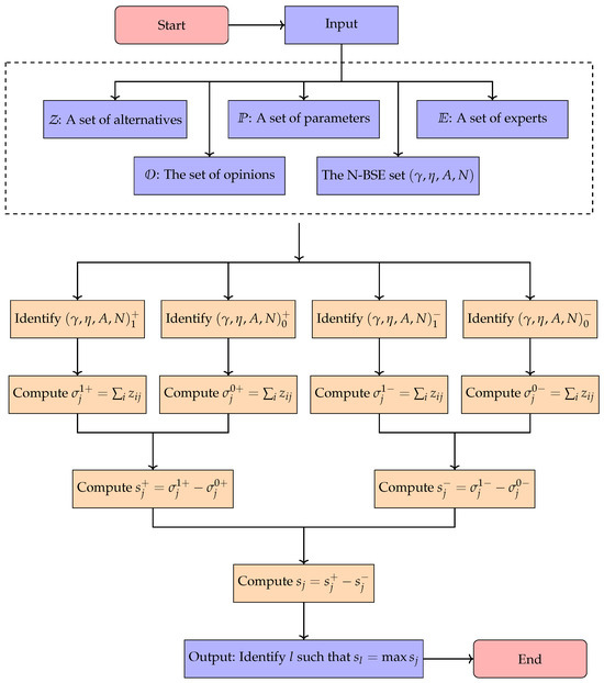
Figure 1.
Flowchart of the proposed algorithm.
4.2. Case Study: Sustainable Energy Solutions
In addressing global challenges like climate change, organizations play a crucial role in advancing sustainable energy solutions. Selecting the most suitable energy project for implementation is a complex task that requires thorough evaluation. A poorly chosen project could lead to inefficiencies and resource wastage, while the right project can foster energy efficiency and environmental sustainability. This example illustrates the process of selecting an optimal energy project.
Suppose a renewable energy company intends to implement one project from a list of seven proposals: . The company forms a committee of experienced employees to prepare a report evaluating the proposals based on key parameters: , along with their negative counterparts: . To finalize the decision, the company shares the report with three energy experts and considers their opinions on the report, as shown in Table 19.
Table 19.
Evaluations of sustainable energy solutions by experts using check-marks.
The check-marks are translated into numerical values (0, 1, 2, 3, 4) for computation, as shown in Example 1.
Therefore, the experts construct a 5-BSE set , as detailed in Table 20.
Table 20.
Evaluations of sustainable energy solutions by experts using 5-BSE set .
For simplicity in the computation process, the experts constructs the tables for positive agree, positive disagree, negative agree, and negative disagree in a straightforward manner, as shown in Table 21, Table 22, Table 23 and Table 24, where represents the entries in these tables.
Table 21.
Tabular representation of a positive agree 5-BSE set .
Table 22.
Tabular representation of a positive disagree 5-BSE set .
Table 23.
Tabular representation of a negative agree 5-BSE set .
Table 24.
Tabular representation of a negative disagree 5-BSE set .
We can easily construct Table 25 by combining the data from Table 21 and Table 22. Similarly, Table 26 can be derived from Table 23 and Table 24.
Table 25.
Positive score table.
Table 26.
Negative score table.
Table 27.
Final score table.
Based on Table 27, we can observe that the maximum score ; thus, the experts will select .
5. Comparative Analysis
This section provides a critical analysis of the proposed N-BSE model, emphasizing its advantages, comparing it with existing approaches, and outlining its limitations. The goal is to evaluate the model’s performance within the context of MAGDM, particularly in situations involving expert input and non-binary evaluations.
5.1. Advantages of the Proposed Model
The proposed N-BSE model offers several significant advantages over existing models in the realm of MAGDM. Key benefits include:
- Comprehensive evaluation: incorporates both positive and negative attributes of alternatives, offering a more balanced and complete assessment.
- Expert opinion integration: aggregates diverse evaluations from multiple experts, ensuring robust and well-rounded DM.
- Non-binary evaluation: allows multi-valued evaluations, providing finer distinctions between alternatives and enhancing DM accuracy.
- Flexibility: applicable across various domains like business, engineering, and healthcare, making it versatile for a wide range of DM problems.
- Transparency: the systematic evaluation process and expert aggregation ensure a transparent and explainable DM framework.
5.2. Comparison with Relevant Existing Approaches
In this subsection, we compare the N-BSE model with several existing approaches, focusing on expert input, evaluation types, and the handling of both positive and negative attributes. The models differ in terms of whether expert input is incorporated, whether bipolarity (the distinction between positive and negative attributes) is considered, and whether evaluations are binary (limited to 0 or 1) or multinary (allowing for more nuanced assessments).
The following Table 28 summarizes these models, showing how they vary in terms of expert input, bipolarity, evaluation type, and the specific methodology for assessing alternatives.
Table 28.
Comparison of N-BSE model with relevant existing approaches.
5.3. Limitations of the Proposed Model
Despite its advantages, the N-BSE model has certain limitations:
- Expert input dependency: the model relies heavily on expert evaluations, which may introduce subjectivity and prove challenging in contexts with limited expert availability.
- Complex aggregation: aggregating multi-valued expert evaluations can be complex and require sophisticated techniques to ensure consistency and accuracy, especially with large datasets.
6. Conclusions and Future Directions
In this paper, we introduced the N-BSE model, a novel approach to MAGDM that integrates expert input, bipolarity, and non-binary evaluations. The N-BSE model provides a comprehensive framework for handling both positive and negative attributes of alternatives, offering a more balanced and nuanced assessment compared to traditional methods. Through the definition of core operations and the presentation of its algebraic properties, we demonstrated the mathematical foundation of the model and its applicability to real-world DM problems. The model’s versatility was highlighted through a case study on selecting sustainable energy solutions, illustrating its ability to aggregate expert opinions and provide optimal decisions in complex, multi-criteria scenarios. A comparative analysis further emphasized the advantages of the N-BSE model, particularly in its ability to handle non-binary evaluations and incorporate diverse expert viewpoints. Overall, the N-BSE model represents a significant advancement in DM frameworks, offering a robust, transparent, and flexible approach to MAGDM that can be applied across various domains.
In the future, we aim to expand our work to include (1) fuzzy N-BSE sets, (2) intuitionistic fuzzy N-BSE sets, (3) Pythagorean fuzzy N-BSE sets, (4) Fermatean fuzzy N-BSE sets, (5) q-rung orthopair fuzzy N-BSE sets, and other related models.
Author Contributions
Conceptualization, S.Y.M.; Methodology, S.Y.M., Z.A.A. and B.A.A.; Formal Analysis, S.Y.M., A.I.A. and B.A.A.; Investigation, A.I.A., B.A.A. and Z.A.A.; Writing Original Draft Preparation, S.Y.M.; Writing Review and Editing, S.Y.M. and Z.A.A.; Funding Acquisition, A.I.A. All authors have read and agreed to the published version of the manuscript.
Funding
This research received no external funding.
Data Availability Statement
All data generated or analyzed during this study are included in this published article.
Acknowledgments
The Researchers would like to thank the Deanship of Graduate Studies and Scientific Research at Qassim University for financial support (QU-APC-2025).
Conflicts of Interest
The authors declare no conflicts of interest.
References
- Zadeh, L.A. Fuzzy sets. Inf. Control 1965, 8, 338–353. [Google Scholar] [CrossRef]
- Goguen, J.A. L-fuzzy sets. J. Math. Anal. Appl. 1967, 18, 145–174. [Google Scholar] [CrossRef]
- Zadeh, L.A. The concept of a linguistic variable and its application to approximate reasoning—I. Inf. Sci. 1975, 8, 199–249. [Google Scholar] [CrossRef]
- Atanassov, K.T. Intuitionistic fuzzy sets. Fuzzy Sets Syst. 1986, 20, 87–96. [Google Scholar] [CrossRef]
- Dubois, D.; Prade, H. Rough fuzzy sets and fuzzy rough sets. Int. J. Gen. Syst. 1990, 17, 191–209. [Google Scholar] [CrossRef]
- Zhang, W.R. Bipolar fuzzy sets and relations: A computational framework for cognitive modeling and multiagent decision analysis. In Proceedings of the First International Joint Conference of the North American Fuzzy Information Processing Society Biannual Conference, San Antonio, TX, USA, 18–21 December 1994; pp. 305–309. [Google Scholar]
- Ramot, D.; Milo, R.; Friedman, M.; Kandel, A. Complex fuzzy sets. IEEE Trans. Fuzzy Syst. 2002, 10, 171–186. [Google Scholar] [CrossRef]
- Torra, V. Hesitant fuzzy sets. Int. J. Intell. Syst. 2010, 25, 529–539. [Google Scholar] [CrossRef]
- Yager, R.R. Pythagorean fuzzy subsets. In Proceedings of the 9th Joint World Congress on Fuzzy Systems and NAFIPS Annual Meeting, Edmonton, AB, Canada, 24–28 June 2013; pp. 57–61. [Google Scholar]
- Cuong, B.C.; Kreinovich, V. Picture fuzzy sets: A new concept for computational intelligence problems. In Proceedings of the Third World Congress on Information and Communication Technologies (WICT 2013), Hanoi, Vietnam, 15–18 December 2013; pp. 1–6. [Google Scholar]
- Gündoğdu, F.K.; Kahraman, C. Spherical fuzzy sets and spherical fuzzy TOPSIS method. J. Intell. Fuzzy Syst. 2019, 36, 337–352. [Google Scholar] [CrossRef]
- Senapati, T.; Yager, R.R. Fermatean fuzzy sets. J. Ambient Intell. Humaniz. Comput. 2020, 11, 663–674. [Google Scholar] [CrossRef]
- Das, S.; Roy, B.K.; Kar, M.B.; Kar, S.; Pamucar, D. Neutrosophic fuzzy set and its application in decision making. J. Ambient Intell. Humaniz. Comput. 2020, 11, 5017–5029. [Google Scholar] [CrossRef]
- Yager, R.R. Generalized orthopair fuzzy sets. IEEE Trans. Fuzzy Syst. 2017, 25, 1222–1230. [Google Scholar] [CrossRef]
- Pawlak, Z. Rough sets. Int. J. Comput. Inf. Sci. 1982, 11, 341–356. [Google Scholar] [CrossRef]
- Pawlak, Z. Hard and soft sets. In Rough Sets, Fuzzy Sets and Knowledge Discovery; Ziarko, W.P., Ed.; Workshops in Computing; Springer: London, UK, 1994. [Google Scholar]
- Molodtsov, D. Soft set theory-first results. Comput. Math. Appl. 1999, 37, 19–31. [Google Scholar] [CrossRef]
- Maji, P.; Biswas, R.; Roy, A. Soft set theory. Comput. Math. Appl. 2003, 45, 555–562. [Google Scholar] [CrossRef]
- Ali, M.I.; Feng, F.; Liu, X.; Min, W.K.; Shabir, M. On some new operations in soft set theory. Comput. Math. Appl. 2009, 57, 1547–1553. [Google Scholar] [CrossRef]
- Maji, P.; Biswas, R.; Roy, A. Fuzzy soft sets. J. Fuzzy Math. 2001, 9, 589–602. [Google Scholar]
- Maji, P.; Biswas, R.; Roy, A. Intuitionistic fuzzy soft sets. J. Fuzzy Math. 2001, 9, 677–692. [Google Scholar]
- Alcantud, J.C.R. Some formal relationships among soft sets, fuzzy sets, and their extensions. Int. J. Approx. Reason. 2016, 68, 45–537. [Google Scholar] [CrossRef]
- Liu, Z.; Alcantud, J.C.R.; Qin, K.; Pei, Z. The relationship between soft sets and fuzzy sets and its application. J. Intell. Fuzzy Syst. 2019, 36, 3751–3764. [Google Scholar] [CrossRef]
- Feng, F.; Fujita, H.; Ali, M.I.; Yager, R.R.; Liu, X. Another view on generalized intuitionistic fuzzy soft sets and related multiattribute decision making methods. IEEE Trans. Fuzzy Syst. 2019, 27, 474–488. [Google Scholar] [CrossRef]
- Al-shboul, A.; Alhazaymeh, K.; Wang, K.L.; Wong, K.B. Fermatean Vague Soft Set and Its Application in Decision Making. Mathematics 2024, 12, 3699. [Google Scholar] [CrossRef]
- Shabir, M.; Naz, M. On bipolar soft sets. arXiv 2013, arXiv:1303.1344. [Google Scholar] [CrossRef]
- Naz, M.; Shabir, M. On fuzzy bipolar soft sets, their algebraic structures and applications. J. Intell. Fuzzy Syst. 2014, 26, 1645–1656. [Google Scholar] [CrossRef]
- Mahmood, T.; Rehman, U.U.; Jaleel, A.; Ahmmad, J.; Chinram, R. Bipolar complex fuzzy soft sets and their applications in decision-making. Mathematics 2022, 10, 1048. [Google Scholar] [CrossRef]
- Fatimah, F.; Rosadi, D.; Hakim, R.F.; R. Alcantud, J.C. Probabilistic soft sets and dual probabilistic soft sets in decision-making. Neural Comput. Appl. 2019, 31, 397–407. [Google Scholar] [CrossRef]
- Zhu, P.; Wen, Q. Probabilistic soft sets. In Proceedings of the IEEE International Conference on Granular Computing, San Jose, CA, USA, 14–16 August 2010; Volume 51, pp. 635–639. [Google Scholar]
- Fatimah, F.; Rosadi, D.; Hakim, R.B.F.; R. Alcantud, J.C. N-soft sets and their decision-making algorithms. Soft Comput. 2018, 22, 3829–3842. [Google Scholar] [CrossRef]
- Shabir, M.; Fatima, J. N-bipolar soft sets and their application in decision making. Preprint 2021. [Google Scholar] [CrossRef]
- Musa, S.Y.; Mohammed, R.A.; Asaad, B.A. N-hypersoft sets: An innovative extension of hypersoft sets and their applications. Symmetry 2023, 15, 1795. [Google Scholar] [CrossRef]
- Musa, S.Y.; Asaad, B.A. Bipolar hypersoft sets. Mathematics 2021, 9, 1826. [Google Scholar] [CrossRef]
- Asaad, B.A.; Musa, S.Y.; Ameen, Z.A. Fuzzy bipolar hypersoft sets: A novel approach for decision-making applications. Math. Comput. Appl. 2024, 29, 50. [Google Scholar] [CrossRef]
- Musa, S.Y. N-bipolar hypersoft sets: Enhancing decision-making algorithms. PLoS ONE 2024, 19, e0296396. [Google Scholar] [CrossRef]
- Musa, S.Y.; Asaad, B.A. A progressive approach to multi-criteria group decision-making: N-bipolar hypersoft topology perspective. PLoS ONE 2024, 19, e0304016. [Google Scholar] [CrossRef]
- Riaz, M.; Razzaq, A.; Aslam, M.; Pamucar, D. M-parameterized N-soft topology-based TOPSIS approach for multi-attribute decision making. Symmetry 2021, 13, 748. [Google Scholar] [CrossRef]
- Musa, S.Y.; Asaad, B.A. Bipolar M-parameterized N-soft sets: A gateway to informed decision-making. J. Math. Comput. Sci. 2025, 36, 121–141. [Google Scholar] [CrossRef]
- Babitha, K.V.; John, S.J. Hesitant fuzzy soft sets. J. New Results Sci. 2013, 3, 98–107. [Google Scholar]
- Khameneh, A.Z.; Kilicman, A. m-polar fuzzy soft weighted aggregation operators and their applications in group decision-making. Symmetry 2018, 10, 636. [Google Scholar] [CrossRef]
- Santos-García, G.; Alcantud, J.C.R. Ranked soft sets. Expert Syst. 2023, 40, e13231. [Google Scholar] [CrossRef]
- Feng, F.; Li, C.; Davvaz, B.; Ali, M.I. Soft sets combined with fuzzy sets and rough sets: A tentative approach. Soft Comput. 2010, 14, 899–911. [Google Scholar] [CrossRef]
- Feng, F.; Liu, X.; Leoreanu-Fotea, V.; Jun, Y.B. Soft sets and soft rough sets. Inf. Sci. 2011, 181, 1125–1137. [Google Scholar] [CrossRef]
- Alcantud, J.C.R.; Khameneh, A.Z.; Santos-García, G.; Akram, M. A systematic literature review of soft set theory. Neural Comput. Appl. 2024, 36, 8951–8975. [Google Scholar] [CrossRef]
- Maji, P.; Biswas, R.; Roy, A. An application of soft sets in a decision-making problem. Comput. Math. Appl. 2002, 44, 1077–1083. [Google Scholar] [CrossRef]
- Chen, D.; Tsang, E.; Yeung, D.S.; Wang, X. The parameterization reduction of soft sets and its applications. Comput. Math. Appl. 2005, 49, 757–763. [Google Scholar] [CrossRef]
- Roy, A.R.; Maji, P. A fuzzy soft set theoretic approach to decision making problems. J. Comput. Appl. Math. 2007, 203, 412–419. [Google Scholar] [CrossRef]
- Feng, F.; Jun, Y.B.; Liu, X.; Li, L. An adjustable approach to fuzzy soft set based decision making. J. Comput. Appl. Math. 2010, 234, 10–20. [Google Scholar] [CrossRef]
- Yang, Y.; Tan, X.; Meng, C. The multi-fuzzy soft set and its application in decision making. Appl. Math. Model. 2013, 37, 4915–4923. [Google Scholar] [CrossRef]
- Khameneh, A.Z.; Kilicman, A. Multi-attribute decision-making based on soft set theory: A systematic review. Soft Comput. 2019, 23, 6899–6920. [Google Scholar] [CrossRef]
- Das, S.; Malakar, D.; Kar, S.; Pal, T. A brief review and future outline on decision making using fuzzy soft set. Int. J. Fuzzy Syst. Appl. 2018, 7, 1–43. [Google Scholar] [CrossRef]
- Alkhazaleh, S.; Salleh, A.R. Soft expert sets. Adv. Decis. Sci. 2011, 2011, 12. [Google Scholar] [CrossRef]
- Alkhazaleh, S.; Salleh, A.R. Fuzzy soft expert set and its application. Appl. Math. 2014, 5, 1349–1368. [Google Scholar] [CrossRef]
- Broumi, S.; Smarandache, F. Intuitionistic fuzzy soft expert sets and its application in decision making. J. New Theory 2015, 1, 89–105. [Google Scholar]
- Ali, G.; Akram, M. Decision-making method based on fuzzy N-soft expert sets. Arab. J. Sci. Eng. 2020, 45, 10381–10400. [Google Scholar] [CrossRef]
- Ulucay, V.; Sahin, M.; Hassan, N. Generalized neutrosophic soft expert set for multiple-criteria decision-making. Symmetry 2018, 10, 437. [Google Scholar] [CrossRef]
- Ali, G.; Akram, M.; Shahzadi, S.; Abidin, M.Z.U. Group decision-making framework with bipolar soft expert sets. J. Mult.-Valued Log. Soft Comput. 2021, 37, 211. [Google Scholar]
- Dalkilic, O.; Demirtaş, N. Combination of the bipolar soft set and soft expert set with an application in decision making. J. Sci. 2022, 35, 644–657. [Google Scholar] [CrossRef]
- Ihsan, M.; Rahman, A.U.; Saeed, M.; Khalifa, H.A.E.W. Convexity-cum-concavity on fuzzy soft expert set with certain properties. Int. J. Fuzzy Log. Intell. Syst. 2021, 21, 233–242. [Google Scholar] [CrossRef]
- Al-Quran, A.; Hassan, N. The complex neutrosophic soft expert set and its application in decision making. J. Intell. Fuzzy Syst. 2018, 34, 569–582. [Google Scholar] [CrossRef]
- Akram, M.; Ali, G.; Alcantud, J.C.R. A novel group decision-making framework under Pythagorean fuzzy N-soft expert knowledge. Eng. Appl. Artif. Intell. 2023, 120, 105879. [Google Scholar] [CrossRef]
- Akram, M.; Ali, G.; Peng, X.; Abidin, M.Z.U. Hybrid group decision-making technique under spherical fuzzy N-soft expert sets. Artif. Intell. Rev. 2022, 55, 4117–4163. [Google Scholar] [CrossRef]
- Zhou, X.; Chen, Y. Multi-attribute decision-making method based on bipolar N-soft expert set. J. Ambient Intell. Humaniz. Comput. 2023, 14, 2617–2630. [Google Scholar] [CrossRef]
- Al-Sharqi, F.; Al-Qudah, Y.; Alotaibi, N. Decision-making techniques based on similarity measures of possibility neutrosophic soft expert sets. Neutrosophic Sets Syst. 2023, 55, 22. [Google Scholar]
- Ihsan, M.; Rahman, A.U.; Saeed, M. Hypersoft expert set with application in decision making for recruitment process. Neutrosophic Sets Syst. 2023, 42, 191–207. [Google Scholar]
- Ali, G.; Afzal, A.; Sheikh, U.; Nabeel, M. Multi-criteria group decision-making based on the combination of dual hesitant fuzzy sets with soft expert sets for the prediction of a local election scenario. Granul. Comput. 2023, 8, 2039–2066. [Google Scholar] [CrossRef]
- Khan, A.; Abidin, M.Z.; Sarwar, M.A. Another view on soft expert set and its application in multi-criteria decision-making. Mathematics 2025, 13, 252. [Google Scholar] [CrossRef]
Disclaimer/Publisher’s Note: The statements, opinions and data contained in all publications are solely those of the individual author(s) and contributor(s) and not of MDPI and/or the editor(s). MDPI and/or the editor(s) disclaim responsibility for any injury to people or property resulting from any ideas, methods, instructions or products referred to in the content. |
© 2025 by the authors. Licensee MDPI, Basel, Switzerland. This article is an open access article distributed under the terms and conditions of the Creative Commons Attribution (CC BY) license (https://creativecommons.org/licenses/by/4.0/).