Article

Curriculum-Enhanced Adaptive Sampling for Physics-Informed Neural Networks: A Robust Framework for Stiff PDEs

1
Department of Electrical and Computer Engineering, Texas A&M University, College Station, TX 77843, USA
2
Artificial Intelligence and Data Science Research Center, Istanbul Technical University, Istanbul 34467, Türkiye
3
Department of Electrical and Computer Engineering, Texas A&M University at Qatar, Doha 23874, Qatar
4
Electrical Engineering Program, College of Science and Engineering, Hamad Bin Khalifa University, Doha 34110, Qatar
5
Chemical Engineering Program, College of Science and Engineering, Hamad Bin Khalifa University, Doha 34110, Qatar
*
Author to whom correspondence should be addressed.
Mathematics 2025, 13(24), 3996; https://doi.org/10.3390/math13243996
Submission received: 30 October 2025 / Revised: 3 December 2025 / Accepted: 8 December 2025 / Published: 15 December 2025
(This article belongs to the Special Issue Physics-Informed Machine Learning: Methodologies and Applications)

Abstract

Physics-Informed Neural Networks (PINNs) often struggle with stiff partial differential equations (PDEs) exhibiting sharp gradients and extreme nonlinearities. We propose a Curriculum-Enhanced (CE) Adaptive Sampling framework that integrates curriculum learning with adaptive refinement to improve PINN training. Our framework introduces four methods: CE-RARG (greedy sampling), CE-RARD (probabilistic sampling), and their novel difficulty-aware dynamic counterparts, CED-RARG and CED-RARD, which adjust refinement effort based on task difficulty. We test these methods on five challenging stiff PDEs: the Allen–Cahn, Burgers’ (I and II), Korteweg–de Vries (KdV), and Reaction equations. Our methods consistently outperform both Vanilla PINNs and curriculum-only baselines. In the most difficult regimes, CED-RARD achieves errors up to 100 times lower for the Burgers’ and KdV equations. For the Allen–Cahn and Reaction equations, CED-RARG proves most effective, reducing errors by over 40% compared to its non-dynamic counterpart and by over two orders of magnitude relative to Vanilla PINN. Visualizations confirm that our methods effectively allocate collocation points to high-gradient regions. By demonstrating success across a wide range of stiffness parameters, we provide a robust and reproducible framework for solving stiff PDEs, with all code and datasets publicly available.

1. Introduction

Rapid advancement of deep learning has transformed numerous scientific disciplines, from computer vision [1] to computational biology [2]. This success has naturally been extended to computational science and engineering, where neural networks are increasingly employed to model complex physical systems governed by partial differential equations (PDEs). Among these approaches, Physics-Informed Neural Networks (PINNs) [3] have emerged as a particularly promising framework that elegantly combines observational data with fundamental physical laws through the direct encoding of PDE constraints into the neural network’s optimization objective [4,5]. PINNs offer several distinct advantages compared to traditional numerical methods. Their mesh-free formulation eliminates the need for complex domain discretization, while their ability to incorporate noisy or incomplete measurement data makes them particularly suitable for real-world applications. Furthermore, PINNs provide a unified framework capable of handling both forward problems (solving PDEs with known parameters) and inverse problems (identifying parameters from data). This versatility has enabled successful applications across diverse domains including fluid dynamics [6], materials science [7], biomedical engineering [8], and climate modeling [9]. PINNs represent a class of deep learning models that integrate governing physical laws, typically expressed as PDEs, into the training process. A PINN typically uses a neural network to approximate the solution to the PDE. Its loss function incorporates not only data-driven terms (like boundary and initial conditions) but also a term that penalizes deviations from the underlying PDE, evaluated at a set of points called collocation or residual points. Automatic differentiation [10,11] is used to compute the derivatives needed for the PDE residual term within the network. This approach enables training even without labelled solution data. Despite these promising developments, significant challenges persist in developing robust and accurate PINN models. A primary limitation arises from the spectral bias inherent in neural networks, which causes them to preferentially learn low-frequency components of the solution. Additional difficulties arise from imbalanced gradient flow during optimization [12] and violations of temporal causality in time-dependent problems [13]. These issues become particularly pronounced when dealing with multi-scale phenomena or solutions containing sharp gradients, often leading to slow convergence or inaccurate results.
Recent research has pursued various strategies to address these challenges. Architectural innovations such as Fourier feature embeddings [14], periodic activation functions [15], and multi-scale or parallel architectures have shown promise in helping networks learn high-frequency functions to mitigate spectral bias. Adaptive training schemes including loss weighting approaches [16], curriculum learning strategies, and sequence-to-sequence (or time-marching) approaches [17] have demonstrated improved optimization behavior. Domain decomposition methods [18,19] have also proven effective in handling complex geometries and multi-physics problems. More recently, hybrid approaches that combine residual-based adaptive refinement with gradient-enhanced PINNs (gPINNs) have been implemented to further enhance convergence and accuracy in regions with steep solution gradients [20].

Problem Overview and Proposed Method

Although promising, standard (or “vanilla”) PINNs often encounter difficulties with complex problems, including stiff PDEs. They can struggle when PDE coefficients related to nonlinear terms or stiffness increase (like high ρ in Allen–Cahn or low ν in Burgers’). These failures might not be caused by the neural network’s inability to represent the solution, but rather from challenges in the optimization process induced by the PDE regularization, potentially making the loss landscape ill-conditioned [17]. Vanilla PINNs using fixed collocation points may not capture sharp gradients [21] and complex solution features effectively. To overcome these limitations, adaptive methods like Residual-based Adaptive Refinement (RAR) have been proposed to focus computational effort on regions with high PDE residuals. While combining RAR with the global-to-local progression of curriculum learning is a logical next step, a simple, static combination of these two powerful techniques is often insufficient. A static approach, which applies a fixed refinement effort at each curriculum stage, fails to account for the sharp increases in difficulty as the problem becomes stiffer. This can lead to an inefficient allocation of computational resources, where easy stages are over-refined and the most critical, difficult stages are under-refined. The core novelty of this work is the introduction of a dynamic, difficulty-aware feedback loop that intelligently modulates the intensity of adaptive sampling in direct response to the curriculum’s progression. We propose using the ratio of mean PDE residuals between successive stages as a lightweight but effective heuristic to quantify the increase in task difficulty. This metric allows our framework to dynamically adjust the number of refinement loops, concentrating computational effort precisely where it is most needed to resolve the challenging physics emerging in stiffer regimes [17]. This approach is purpose-built for finding a highly accurate solution to a single, difficult PDE instance, a goal distinct from generalization-focused meta-learning methods that also use difficulty metrics [22]. The major technical contributions of this work are:
  • We propose a novel curriculum-enhanced adaptive sampling framework for PINNs, which dynamically integrates curriculum learning with residual-based adaptive refinement. By progressively introducing stiffness through the curriculum regularization while adaptively refining collocation points based on PDE residuals, our approach robustly resolves sharp gradients and stiff regions.
  • We introduce four adaptive sampling algorithms: Curriculum-Enhanced RAR-Greedy (CE-RARG), Curriculum-Enhanced RAR-Distribution (CE-RARD), and their novel difficulty-aware counterparts, CED-RARG and CED-RARD. The difficulty-aware variants employ a stiffness-adaptive scheme that dynamically adjusts the number of refinement loops for each curriculum stage based on its relative difficulty.
  • Through systematic experiments on five challenging stiff PDE systems (the Allen–Cahn, Burgers’ I, Burgers’ II, Korteweg–de Vries, and Reaction equations) across varying nonlinearity regimes, we demonstrate that our methods dramatically outperform standard PINNs and curriculum-only approaches. Notably, CED-RARD achieves error reductions of up to two orders of magnitude on the Burgers’ and KdV equations, while CED-RARG proves most effective on the Allen–Cahn and Reaction problems.
  • We provide a publicly available implementation, including code, datasets, and reference solutions to ensure full reproducibility and facilitate future research in PINNs for stiff PDEs.

2. Materials and Methods

2.1. Physics-Informed Neural Networks

PINNs are deep learning models designed to solve PDEs by embedding the PDE constraints directly into the loss function. Unlike traditional numerical methods that discretize the domain and solve the equations iteratively, PINNs exploit the universal approximation capabilities of neural networks to provide continuous approximations of PDE solutions.
Consider a PDE defined over a spatial-temporal domain Ω × ( 0 , T ] with boundary Ω and initial time t = 0 . The PDE is expressed as
F [ u ] = 0 in Ω × ( 0 , T ] ,
with the boundary condition
u = g on Ω × ( 0 , T ] ,
and the initial condition
u = h in Ω at t = 0 ,
where F is a differential operator, u denotes the unknown solution, g represents the prescribed boundary data, and h stands for the initial data. The goal of a PINN is to approximate the solution u with a neural network u ^ ( x , t ; θ ) , where x and t are the spatial and temporal coordinates, respectively, and θ denotes the trainable parameters. The training process is guided by a composite loss function designed to enforce the PDE, the boundary condition, and the initial condition. First, the PDE residual loss is defined as the mean squared error (MSE) of the PDE residual computed at a set of collocation points y i Ω × ( 0 , T ] :
L PDE ( θ ) = 1 N r i = 1 N r F u ^ ( y i ; θ ) 2 ,
where N r is the number of collocation points. The boundary condition loss, ensuring that the network output matches the prescribed boundary data at points z i Ω × ( 0 , T ] , is captured through:
L BC ( θ ) = 1 N b i = 1 N b u ^ ( z i ; θ ) g ( z i ) 2 ,
with N b representing the number of boundary points. The initial condition loss, which enforces the initial condition at t = 0 for points x i Ω , is expressed as
L IC ( θ ) = 1 N 0 i = 1 N 0 u ^ ( x i , 0 ; θ ) h ( x i ) 2 ,
where N 0 is the number of points used to enforce the initial condition. The total loss function that the network minimizes is the sum of these three components:
L PINN ( θ ) = L PDE ( θ ) + L BC ( θ ) + L IC ( θ ) .
The network parameters θ are optimized using gradient-based methods such as Adam or L-BFGS-B [23]. Automatic differentiation is employed to compute the necessary derivatives efficiently, ensuring that the PDE residual is accurately evaluated. Figure 1 schematically illustrates the PINN framework. In this approach, the network accepts spatial and temporal inputs to produce an output u. This output is used to calculate the PDE residual, boundary condition, and initial condition losses, which are then combined and minimized to approximate the solution to the PDE.

2.2. Curriculum Learning in PINNs

Curriculum learning has emerged as a powerful strategy for improving PINN training, particularly for challenging problems where direct optimization does not converge to physically meaningful solutions. The core idea involves decomposing the learning task into a sequence of progressively more difficult subtasks, allowing the model to first learn simpler patterns before tackling more complex aspects. In the context of PINNs, ref. [17] demonstrated that curriculum regularization can significantly improve performance by initially training the network with simplified PDE coefficients (e.g., smaller convection or reaction terms) and gradually increasing them to the target values. This approach helps overcome optimization challenges associated with complex loss landscapes that arise when directly training with large PDE coefficients. The work [17] showed that curriculum learning could reduce errors by 1–2 orders of magnitude compared to standard PINN training, particularly for problems involving convection, reaction, and Reaction–Diffusion systems. Building on these insights, Wang et al. [24] proposed an enhanced curriculum training strategy for time-dependent PDEs and singular perturbation problems. Their approach involves temporal domain decomposition, where the solution is learned sequentially across time windows, with each subsequent window using the prediction from the previous time-step as its initial condition. This method respects the causal structure of time-dependent systems while reducing the optimization difficulty of learning the full evolution simultaneously.
The effectiveness of curriculum learning in PINNs can be attributed to multiple factors. First, it provides better initialization for subsequent training stages. Second, it enables the network to learn smoother solutions before addressing high-frequency features. Additionally, it helps avoid poor local minima in PINNs’ complex loss landscape. Finally, it ensures physical consistency is maintained throughout the training process.
For problems with parameter-dependent behavior (e.g., varying Reynolds numbers in fluid dynamics), curriculum learning has proven particularly valuable. As shown in [24], starting training at lower Reynolds numbers and progressively increasing to the target value enables PINNs to successfully model complex flow phenomena that would otherwise be inaccessible through direct training. The success of curriculum learning in PINNs aligns with broader findings in machine learning [25], demonstrating that curriculum-based training strategies can significantly improve model performance and convergence across various domains. In scientific machine learning specifically, curriculum approaches have become an essential tool for tackling challenging PDE problems where traditional PINN formulations struggle.

2.3. Residual-Based Adaptive Sampling Methods

The Residual-Based Adaptive Refinement (RAR) algorithm is a greedy strategy that adaptively introduces new collocation points in regions where the PDE residual is high. Originally proposed in [26], RAR has proven effective for solving PDEs with sharp gradients or localized features. The RAR-G variant begins by uniformly sampling an initial set of collocation points across the domain. A PINN is then trained for a fixed number of iterations. In each refinement cycle, a dense set of candidate points is uniformly sampled, and the corresponding PDE residuals (defined as the absolute value of the residual function) are computed. The algorithm then selects a fixed number of points with the highest residuals and adds them to the training set. The PINN is retrained using the augmented dataset, and this process repeats until a specified stopping criterion is satisfied. The defining feature of RAR-G is its greedy selection of high-residual points, which enables efficient learning in regions with steep gradients or discontinuities [27]. The RAR-D (Residual-Based Adaptive Refinement with Distribution) algorithm enhances the sampling process by using a probabilistic strategy rather than a purely greedy approach [27]. It generalizes several recent adaptive sampling methods [28,29,30,31] and proceeds as follows. The algorithm starts by uniformly sampling an initial set of collocation points and training the PINN for a specified number of iterations. In each refinement step, PDE residuals are computed over the domain. These residuals are used to define a probability density function, following  [27]:
p ( x ) ε k ( x ) E [ ε k ( x ) ] + c ,
where k 0 and c 0 are tunable parameters. New collocation points are then sampled according to this distribution, prioritizing regions with high residuals while preserving sampling diversity. These points are added to the training set, and the model is retrained. This process is repeated until a predefined stopping criterion is met. The RAR-D method enables more flexible refinement than purely greedy approaches [27].

2.4. Curriculum-Enhanced Adaptive Sampling

We introduce four novel algorithms that integrate curriculum learning with residual-based adaptive refinement to improve the training of PINNs on challenging PDEs. Each method combines a curriculum regularization with either a greedy or probabilistic point refinement strategy:
  • CE-RARG (outlined in Algorithm 1) adds a fixed number of residual-based collocation points at each curriculum stage using a greedy strategy. It focuses on areas with the highest residuals.
  • CED-RARG extends CE-RARG by adjusting the number of added high residual points dynamically based on task difficulty estimates.
  • CE-RARD (outlined in Algorithm 2) uses a probabilistic sampling strategy based on residuals to select collocation points for each stage, maintaining consistency with the curriculum.
  • CED-RARD builds on CE-RARD by dynamically adjusting the number of refinement loops per stage based on the ratio of mean residuals between successive tasks.
  These methods improve training efficiency by combining adaptive sampling with curriculum-based learning. CE/CED-RARG use point selection based on residual magnitudes (greedy refinement), while CE/CED-RARD rely on residual-informed distributions to sample points.
As shown in Algorithm 3, CED-RARG integrates curriculum learning with a dynamic, greedy refinement process. The training is divided into a curriculum of m stages ordered by increasing difficulty (e.g., by varying a PDE parameter like ρ or ν ). At each stage, the algorithm first performs an initial training phase. It then dynamically adapts the number of refinement iterations for that stage, N_rar_loops, based on the ratio of the current mean residual to that of the previous stage. This dynamic allocation of the computational budget is a key feature of the CED approach. When a curriculum stage proves to be more difficult, the algorithm automatically performs more refinement loops. Consequently, a greater total number of high-residual points are added for that stage, enabling a more intensive and targeted refinement compared to fixed-loop approaches [20,27]. Within each of these refinement loops, a set number of new points, k, is calculated as a fixed ratio of the current training set size. The algorithm then greedily selects these k new points from a dense candidate set by identifying the locations with the highest residuals. These points are added to the training set, and the model continues training for a fixed number of epochs (N_rar_epochs). This process adaptively concentrates computational effort on the most challenging regions, and the intensity of this refinement is scaled based on the difficulty of progression between curriculum stages.
Algorithm 1 CE-RARG: RAR with Curriculum Learning
1:
Hyperparameters: Fixed ratio RATIO, epoch counts N i n i t i a l _ e p o c h s , N r a r _ e p o c h s , loop count N r a r _ l o o p s .
2:
Define a curriculum of m stages, ordered by increasing difficulty (e.g., by ρ ).
3:
Initialize PINN model and sample initial training set T .
4:
for each stage i = 1 to m do
5:
      Set PDE parameters for stage i.
6:
      Train PINN on current set T for N i n i t i a l _ e p o c h s .       ▹ Initial training for the new stage
7:
      for iteration j = 1 to N r a r _ l o o p s  do
8:
            Sample dense candidate set S 0 of n s a m p l i n g points.
9:
            Compute residuals ε ( x ) = | f ( x ; u ^ ( x ) ) | for all x S 0 .
10:
          Set number of points to add k = RATIO × | T | .
11:
          Select k points S from S 0 with the highest residuals.
12:
          Augment training set: T T S .
13:
          Continue training PINN on set T for a fixed N r a r _ e p o c h s epochs.
14:
    end for
15:
end for
16:
Save final model and results.
Algorithm 2 CE-RARD: RARD with Curriculum Learning
1:
Hyperparameters: Fixed ratio RATIO, epoch counts N i n i t i a l _ e p o c h s , N r a r _ e p o c h s , loop count N r a r _ l o o p s .
2:
Define a curriculum of m stages, ordered by increasing difficulty (e.g., by ρ ).
3:
Initialize PINN model and sample initial training set T .
4:
for each stage i = 1 to m do
5:
      Set PDE parameters for stage i.
6:
      Train PINN on current set T for N i n i t i a l _ e p o c h s .       ▹ Initial training for the new stage
7:
      for iteration j = 1 to N r a r _ l o o p s  do
8:
            Sample dense candidate set S 0 of n s a m p l i n g points.
9:
            Compute residuals ε ( x ) for all x S 0 .
10:
          Define a sampling distribution p ( x ) over S 0 based on residuals, as in Equation (8).
11:
          Set number of points to sample k = RATIO × | T | .
12:
          Sample k new points S from S 0 according to the distribution p ( x ) .
13:
          Augment training set: T T S .
14:
          Continue training PINN on set T for a fixed N r a r _ e p o c h s epochs.
15:
    end for
16:
end for
17:
Save final model and results.
In contrast, CED-RARD (outlined in Algorithm 4) replaces this greedy selection with a residual-informed sampling strategy. Like CED-RARG, it operates over a predefined curriculum and, crucially, also dynamically adjusts the number of refinement loops (N_rar_loops) based on inter-stage difficulty. By increasing the number of refinement cycles for harder tasks, it ensures that a larger total number of points are sampled from its residual-informed probability distribution (see Equation (8)). This distribution prioritizes regions with high residuals, a strategy proven effective for enhancing solution accuracy by adaptively adding points where the error is largest, especially for solutions with steep gradients [20,27]. By merging the progressive structure of curriculum learning with residual-driven probabilistic sampling, CED-RARD aims to solve complex PDEs more efficiently by focusing refinement where needed while maintaining domain-wide coverage.
Algorithm 3 CED-RARG: Dynamic RARG with Curriculum Learning
1:
Hyperparameters: Fixed ratio RATIO, epoch counts N i n i t i a l _ e p o c h s , N r a r _ e p o c h s , base loop count N b a s e _ l o o p s , scaling exponent α .
2:
Define a curriculum of m stages, ordered by increasing difficulty.
3:
Initialize PINN model and sample initial training set T .
4:
for each stage i = 1 to m do
5:
      Set PDE parameters for stage i.
6:
      Train PINN on current set T for N i n i t i a l _ e p o c h s .       ▹ Initial training for the new stage
7:
      Compute the mean residual for the current stage, ε i .
8:
      if  i = 1  then
9:
          Set N r a r _ l o o p s N b a s e _ l o o p s .             ▹ Use base loops for the first stage
10:
    else
11:
          Set N r a r _ l o o p s round ( N b a s e _ l o o p s × ( ε i / ε i 1 ) α ) .     ▹ Scale loops by difficulty ratio
12:
    end if
13:
    for iteration j = 1 to N r a r _ l o o p s  do
14:
        Sample dense candidate set S 0 of n s a m p l i n g points.
15:
        Compute residuals ε ( x ) = | f ( x ; u ^ ( x ) ) | for all x S 0 .
16:
        Set number of points to add k = RATIO × | T | .
17:
        Select k points S from S 0 with the highest residuals.
18:
        Augment training set: T T S .
19:
        Continue training PINN on set T for a fixed N r a r _ e p o c h s epochs.
20:
    end for
21:
end for
22:
Save final model and results.
Algorithm 4 CED-RARD: Dynamic RARD with Curriculum Learning
1:
Hyperparameters: Fixed ratio RATIO, epoch counts N i n i t i a l _ e p o c h s , N r a r _ e p o c h s , base loop count N b a s e _ l o o p s , scaling exponent α .
2:
Define a curriculum of m stages, ordered by increasing difficulty (e.g., by ρ ).
3:
Initialize PINN model and sample initial training set T .
4:
for each stage i = 1 to m do
5:
      Set PDE parameters for stage i.
6:
      Train PINN on current set T for N i n i t i a l _ e p o c h s .       ▹ Initial training for the new stage
7:
      Compute the mean residual for the current stage, ε i .
8:
      if  i = 1  then
9:
          Set N r a r _ l o o p s N b a s e _ l o o p s .             ▹ Use base loops for the first stage
10:
    else
11:
          Set N r a r _ l o o p s round ( N b a s e _ l o o p s × ( ε i / ε i 1 ) α ) .     ▹ Scale loops by difficulty ratio
12:
    end if
13:
    for iteration j = 1 to N r a r _ l o o p s  do
14:
          Sample dense candidate set S 0 of n s a m p l i n g points.
15:
          Compute residuals ε ( x ) for all x S 0 .
16:
          Define a sampling distribution p ( x ) over S 0 based on residuals, as in Equation (8).
17:
          Set number of points to sample k = RATIO × | T | .
18:
          Sample k new points S from S 0 according to the distribution p ( x ) .
19:
          Augment training set: T T S .
20:
          Continue training PINN on set T for a fixed N r a r _ e p o c h s epochs.
21:
    end for
22:
end for
23:
Save final model and results.
Our choice to use the ratio of mean PDE residuals as a difficulty metric is grounded in the fundamental principles of PINNs and adaptive sampling literature. The PDE residual quantifies the extent to which the network’s output fails to satisfy the governing physical laws, and a high residual in specific regions is a well-established indicator of task difficulty [27]. This heuristic is further validated by analyzing the spectral properties of the exact solution. For instance, a 2D FFT of the Burgers’ equation solution reveals that as the curriculum progresses to lower viscosity values, the energy concentrated in high-frequency bands increases significantly. This confirms that our residual-based ratio is a reliable proxy for the intrinsic increase in solution complexity and high-frequency content, directly addressing the core challenge of spectral bias. This principle forms the basis of many successful adaptive sampling methods, such as RAR, which focus computational effort on high-residual areas. In a curriculum learning framework, however, the challenge is to measure the relative increase in difficulty when transitioning between stages. Our proposed ratio, r i = ε i / ε i 1 , where ε is the mean residual, is designed specifically for this purpose. A large ratio ( r i 1 ) signals a significant jump in problem stiffness, justifying a corresponding increase in the number of refinement loops to resolve the new, more challenging physics [26]. While more complex difficulty metrics exist, such as those based on gradient similarity in meta-learning frameworks like DATS [22], they are computationally more expensive and designed for a different goal (optimizing generalization across a family of PDEs). Our heuristic is deliberately lightweight and direct, making it an ideal and computationally inexpensive indicator for guiding the sequential, single-task curriculum of our CED- methods.
The distribution in (8) enables a tunable trade-off between exploitation by assigning higher probabilities to points with large residuals (via larger k) and exploration by maintaining diversity in sampling (via parameter c). By merging the progressive structure of curriculum learning with residual-driven probabilistic sampling, CED-RARD aims to solve complex PDEs more efficiently, focusing refinement where needed while maintaining domain-wide coverage.

3. Experiments

To rigorously validate the robustness of our framework and account for the inherent stochasticity of neural network training, all reported error metrics are the mean values obtained from 5 independent runs, each with a different random seed. While a larger number of runs would typically be required for a full statistical analysis including standard deviations, the computational expense of our multi-stage curriculum framework makes this prohibitive. More importantly, our curriculum-based approach is specifically designed to stabilize the optimization process. It has been shown that curriculum regularization not only decreases error but also reduces the variance of the error compared to standard PINN training [17]. The low variance we observed across our runs supports this hypothesis, confirming the stability of our framework.
We evaluate our proposed methods on several PDE benchmarks: the 1D Allen–Cahn equation, the 1D Burgers’ equation, a Korteweg–de Vries equation, and a pure Reaction equation. Curriculum learning is applied in all cases to guide the training process progressively. PINN models are implemented using the DeepXDE library [26] with a PyTorch backend. Each model consists of three hidden layers with 64 neurons per layer, using tanh ( x ) as the activation function. The weights are initialized with the Glorot (Xavier) scheme [32]. For all methods, training begins with an initial set of 5000 collocation points uniformly sampled from the domain. The initial training phase consists of 15,000 steps using Adam [33] with a learning rate of 0.001, followed by an additional 15,000 steps of fine-tuning with the L-BFGS-B optimizer [23]. Subsequently, training proceeds iteratively over 50 refinement loops. In each iteration, new collocation points are added to the training set, after which the model is further optimized with 1000 Adam steps followed by 1000 L-BFGS-B steps. This refinement process is consistently applied across all proposed algorithms.
In our experimental setup, the baseline CE-RARG/RARD methods use a fixed number of N_rar_loops = 50 refinement iterations for each curriculum stage. In contrast, the CED-RARG/RARD methods dynamically determine the number of refinement loops based on task difficulty, as described in Algorithm 3. For both sets of methods, within each refinement loop, a number of new points, k, is added based on a fixed proportion (RATIO) of the current training set size ( k = RATIO × | T | ). We use a RATIO of 0.005 for all experiments. This framework ensures a fair comparison between the fixed-loop (CE) and dynamic-loop (CED) strategies, as both begin with the same initial 5000 points and use an identical point-addition mechanism.
For CE/CED-RARD, points are sampled according to the residual density function defined in Equation (8), implementing a residual-based distribution sampling strategy. Following the recommendations in [27], we set k = 2 and c = 0 for all PDEs implemented in this paper: the Allen–Cahn, Burgers-I, Burgers-II, KdV, and Reaction equations. Furthermore, the number of new points added in each loop is determined by RATIO = 0.005, an empirical value [27] found to be effective for the proportional sampling strategy used in our work. The surrogate function of each PDE is implemented as an output transformation within the DeepXDE framework.
To assess accuracy, we compare the PINN predictions against reference solutions computed using the Chebfun [34] package in MATLAB (R2024a), which provides high-precision solutions via Chebyshev polynomial interpolation. Model performance is quantified using the Relative L 2 Error, which measures the average normalized difference between the predicted solution u and the reference solution u ref :
L 2 = 1 N i = 1 N u ( x i ) u ref ( x i ) 2 u ref ( x i ) 2 ,
where x i denotes the spatial or temporal coordinates.

3.1. Allen–Cahn Equation

The Allen–Cahn equation describes phase separation phenomena, and its stiffness often increases with the coefficient ( ρ ) of its nonlinear term. The specific form studied is:
u t = D 2 u x 2 + ρ ( u u 3 ) , x [ 1 , 1 ] , t [ 0 , 1 ]
IC : u ( 0 , x ) = x 2 cos ( π x ) BC : u ( t , 1 ) = u ( t , 1 ) = 1 Surrogate : u ^ ( t , x ) = x 2 cos ( π x ) + t ( 1 x 2 ) u ( t , x ; θ )
where u ( x , t ) denotes the unknown solution of PDE, D is the diffusion coefficient (e.g., D = 0.001 ), and ρ is the coefficient varied to change stiffness (e.g., ρ = 5 to 10) and u ( x , t , θ ) represents the output of the neural network. The surrogate function enforces the initial and boundary conditions through its construction. For this equation, we progressively increase the nonlinear term coefficient ρ from 5 to 10 under defined initial and boundary conditions. As shown in Table 1, the non-curriculum methods fail as ρ increases: Vanilla PINN’s error becomes unacceptably large at ρ = 7 , while both RAR-G and RAR-D fail at ρ = 8 , exhibiting a sudden error increase of nearly two orders of magnitude. In contrast, CE-Vanilla successfully limits this growth, achieving a nearly 30-fold lower error than Vanilla at ρ = 10 , though its error still trails the best-performing methods by a factor of 5–6. The curriculum-based adaptive methods demonstrate the most robust performance. CE-RARG and CED-RARG both maintain low, stable errors across all nonlinearities. Notably, CED-RARG delivers superior performance at the highest stiffness, cutting CE-RARG’s error by over 40% at ρ = 10 and securing the lowest overall error for ρ 9 . This performance gain comes from its adaptive nature. As the nonlinearity increases, CED-RARG identifies the increasing difficulty and allocates more refinement loops to these harder stages. This allows it to consider a larger total number of high-residual points along the sharp phase transition fronts, ensuring they are resolved with high fidelity. While the performance of CE-RARD degrades by an order of magnitude as stiffness increases—its fixed number of refinement loops proving insufficient—its difficulty-aware counterpart, CED-RARD, successfully mitigates this drop by dynamically increasing its refinement effort, thus maintaining stable and competitive accuracy. Overall, the difficulty-aware schemes (CED-RARG and CED-RARD) offer the most resilient performance against increasing nonlinearity precisely because they adaptively concentrate computational effort where it is most needed.
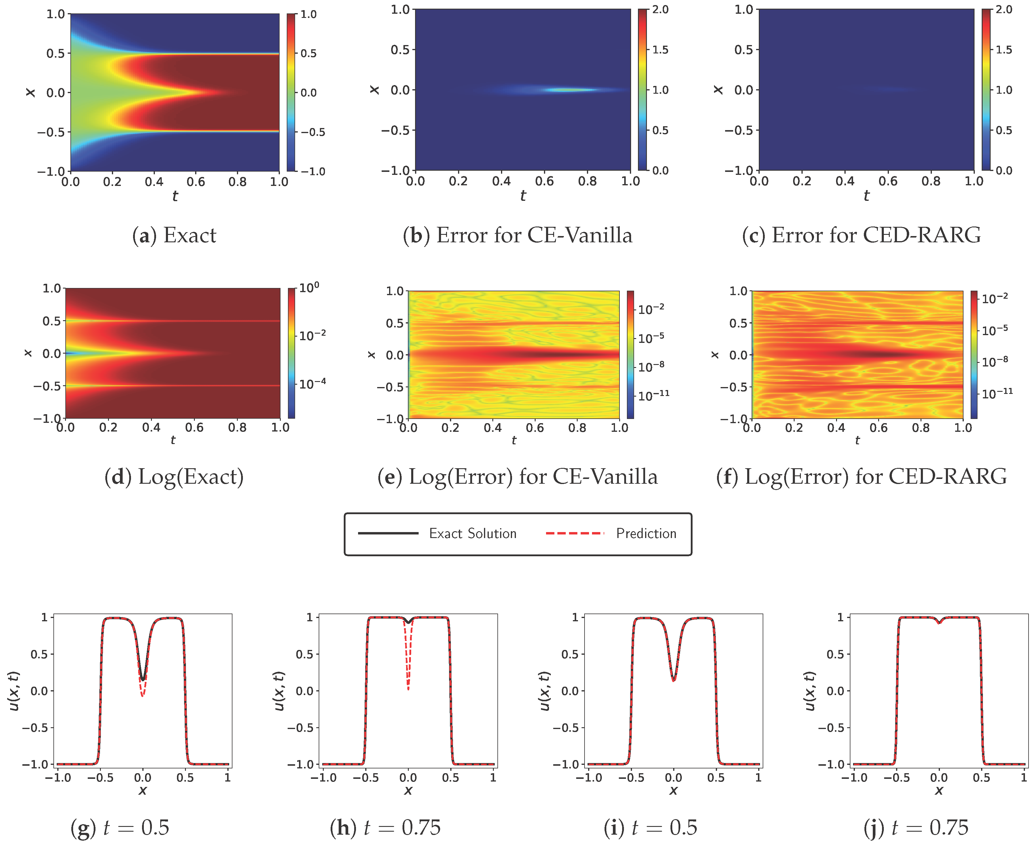
Figure 2 clearly illustrates the performance difference between CED-RARG and CE-Vanilla, supporting the quantitative results and highlighting the improved accuracy achieved by CED-RARG. The absolute error plots (Figure 2b,c) reveal that CE-Vanilla exhibits significantly larger and more widespread errors across the spatial domain, particularly in regions of sharp transitions, while CED-RARG maintains much tighter error control. The time slices (Figure 2d–g) tell the same story: at both t = 0.50 and t = 0.75 , CE-Vanilla’s solutions show noticeable deviations from the exact profile, including artificial dips and amplitude mismatches. In contrast, CED-RARG’s solutions closely match the reference solution, preserving the correct waveform structure even at later time steps. This visual analysis confirms that the difficulty-aware adaptive sampling in CED-RARG reduces global error metrics by ensuring more physically faithful solutions in challenging high-nonlinearity regimes.
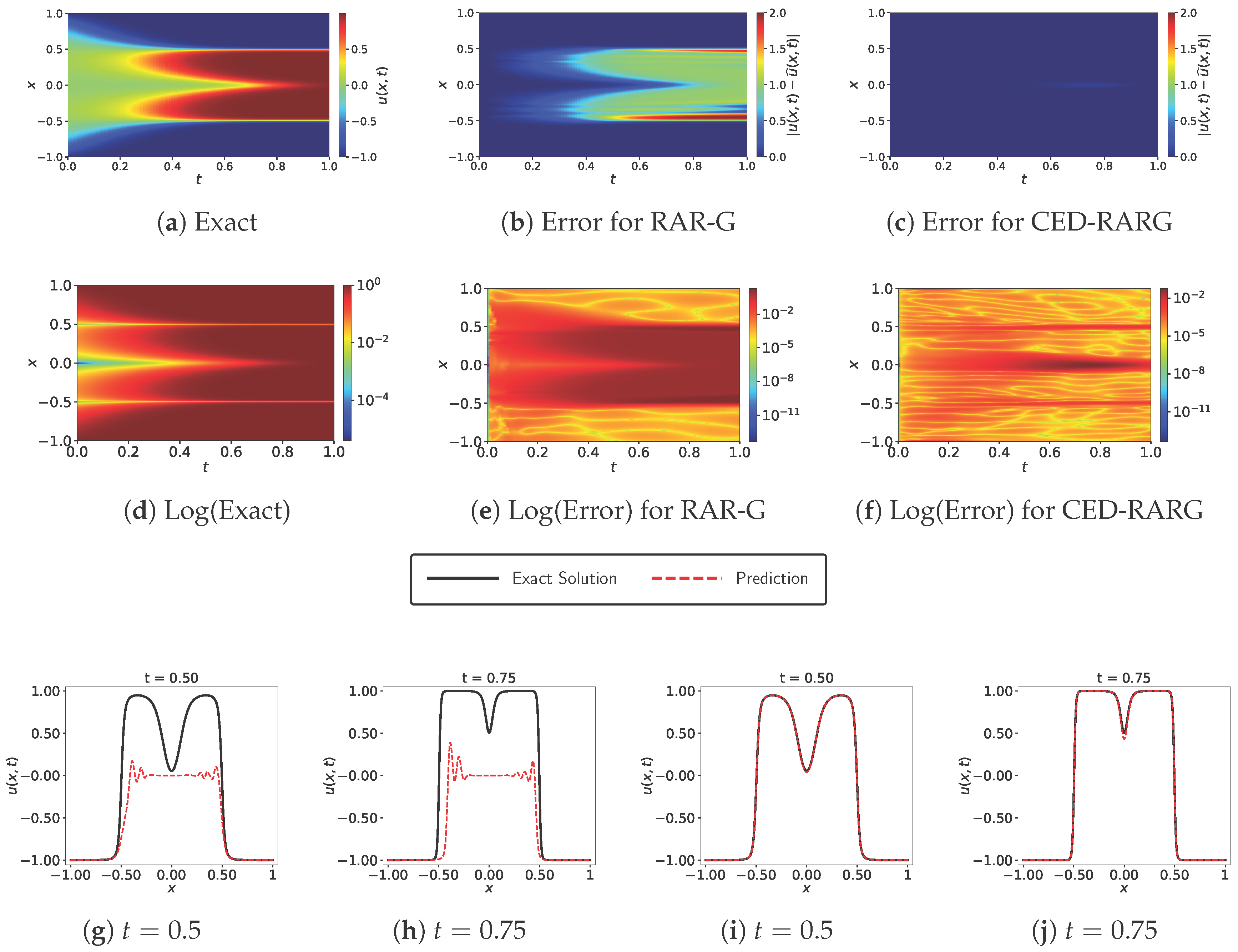
Figure 3 provides a compelling visual analysis of performance at the critical parameter ρ = 8 , where the non-curriculum adaptive method RAR-G begins to fail. The absolute error plots (Figure 3b,c) reveal a stark contrast: RAR-G suffers from large, widespread errors concentrated along the solution’s transition fronts, whereas the error for CED-RARG is orders of magnitude smaller and remains negligible across the entire domain. This performance disparity is further detailed in the solution slices. At t = 0.75 (Figure 3e), the RAR-G prediction completely fails, producing a flattened and distorted waveform that does not capture neither the amplitude nor the shape of the exact solution. Conversely, the CED-RARG prediction at the same time slice (Figure 3g) is visually indistinguishable from the exact profile, perfectly preserving the waveform’s structure. This visual evidence confirms that the curriculum-based framework is essential for stabilizing the training, allowing the difficulty-aware sampling of CED-RARG to succeed where a simpler adaptive method like RAR-G completely breaks down.

3.2. Ablation Study: Computational Cost vs. Accuracy for Static (CE-) and Dynamic (CED-) Strategies

To address the trade-off between computational cost and accuracy, we perform an ablation study comparing our static (CE-) and dynamic (CED-) methods, using the Allen–Cahn equation as a representative case study. The primary difference lies in the allocation of computational effort: the static CE-RARG method uses a fixed number of 300 refinement loops across the entire curriculum, whereas the dynamic CED-RARG method adjusts the number of loops based on inter-stage difficulty. As summarized in Table 2, the dynamic approach results in a higher computational cost. CED-RARG performs approximately 500 total refinement loops, leading to the addition of roughly 12,500 high-residual points and an increase in total training duration of about 30% compared to the static CE-RARG method, which adds only 7500 points. However, this increased investment yields a substantial improvement in accuracy. At the most challenging stage ( ρ = 10 ), CED-RARG reduces the final L2 error by over 40% compared to its static counterpart. This demonstrates that our dynamic framework provides a more efficient use of computational resources. By intelligently concentrating refinement in the most difficult stages, it achieves a level of accuracy that the static method cannot reach, validating the trade-off of a modest increase in computational cost for a significant gain in solution fidelity.

3.3. Ablation Study on Stability and Robustness

To quantitatively assess the stability and robustness of our proposed framework, we conducted an extensive ablation study on the Allen–Cahn equation at its most challenging stage ( ρ = 10 ). We performed 30 independent runs for each method with different random seeds. The results, summarized in Table 3, provide definitive evidence for the stabilization effect of our curriculum-enhanced adaptive methods.
The non-curriculum methods (Vanilla, RAR-G, RAR-D) not only produce high mean errors but also exhibit large standard deviations (on the order of 10 2 ), indicating highly unstable training outcomes. While a simple curriculum (CE-Vanilla) improves stability, reducing the standard deviation by an order of magnitude to 3.53 × 10 3 , our proposed adaptive methods achieve a much higher degree of robustness.
In particular, the best-performing methods, CE-RARG and CED-RARG, have standard deviations of only 5.07 × 10 4 and 2.86 × 10 4 , respectively. This is more than 10 times lower than the CE-Vanilla baseline and more than 150 times lower than the standard Vanilla PINN. This drastic reduction in variance directly supports the claim that our framework stabilizes training and leads to reliable, reproducible solutions for stiff PDEs. Although the main results in this paper are averaged over 5 runs due to prohibitive computational costs, this targeted study provides a clear and robust validation of our approach.

3.4. Burgers’ Equation-I

The Burgers’ equation is a fundamental PDE that describes phenomena such as shock waves and fluid flow, where its stiffness relates to the viscosity coefficient ( ν ). The 1D form studied is:
u t + u u x = ν 2 u x 2 , x [ 1 , 1 ] , t [ 0 , 1 ]
IC : u ( 0 , x ) = sin ( π x ) BC : u ( t , 1 ) = u ( t , 1 ) = 0 Surrogate : u ^ ( t , x ) = sin ( π x ) + t ( 1 x 2 ) u ( t , x ; θ )
where u ( x , t ) is the velocity field, and ν is the kinematic viscosity, varied to change stiffness and u ( x , t , θ ) is the output of neural network constructed in PINNs. The surrogate combines hard constraints for BCs with an exponentially decaying IC term. As shown in Table 4, for this equation, we gradually reduce the viscosity parameter ν from 0.009 / π to 0.003 / π . Problem difficulty increases as ν decreases, and all methods exhibit this trend. The non-curriculum methods (Vanilla, RAR-G, RAR-D) fail dramatically, with errors expanding by over three orders of magnitude and becoming unacceptably large for ν 0.008 / π . While CE-Vanilla improves upon the baseline, its performance is unstable, and its error still exceeds 10 1 at the lowest viscosity. In contrast, all four curriculum-enhanced adaptive methods maintain robust performance, with errors staying below 10 2 across the entire range. Among them, CED-RARD emerges as the top-performing method. Its success is a direct result of its difficulty-aware design. As the viscosity decreases and the problem becomes stiffer, CED-RARD detects the increasing task difficulty and automatically increases its number of refinement loops. This ensures that a larger total number of high-residual points are added precisely where the shock front is sharpest, allowing it to maintain the lowest error across all viscosity levels and achieve a final error of just 2.3 × 10 3 . The other adaptive methods (CE-RARG, CED-RARG, and CE-RARD) are also highly effective, reducing the final error by over 95% compared to CE-Vanilla, but CED-RARD’s dynamic allocation of refinement effort proves most robust.
Figure 4 provides visual evidence of CED-RARD’s superior performance over CE-Vanilla at the challenging viscosity level of ν = 0.003 / π . The absolute error plots Figure 4b,c show that CE-Vanilla accumulates catastrophic errors concentrated around the shock front, with amplitudes nearly two orders of magnitude higher than those of CED-RARD. The time slices Figure 4d–g further confirm this. At t = 0.75 (Figure 4e vs. Figure 4g), CE-Vanilla’s solution is completely distorted, failing to capture the shock’s shape and amplitude. In contrast, CED-RARD maintains high fidelity to the reference solution, resolving the steep gradient with only minor deviations. This visual analysis confirms that CED-RARD’s difficulty-aware adaptive sampling effectively concentrates points in critical regions, leading to sharp shock resolution and robust preservation of the solution’s structure. The results demonstrate that combining residual-based distribution sampling with curriculum learning yields a far more robust solver than standard curriculum strategies alone.

3.5. Burgers’ Equation-II

We also investigated a second case of the Burgers’ equation, featuring a more challenging initial condition with a higher spatial frequency. The 1D form studied is:
u t + u u x = ν 2 u x 2 , x [ 1 , 1 ] , t [ 0 , 1 ] IC : u ( 0 , x ) = sin ( 2 π x ) BC : u ( t , 1 ) = u ( t , 1 ) = 0 Surrogate : u ^ ( t , x ) = sin ( 2 π x ) + t ( 1 x 2 ) u ( t , x ; θ )
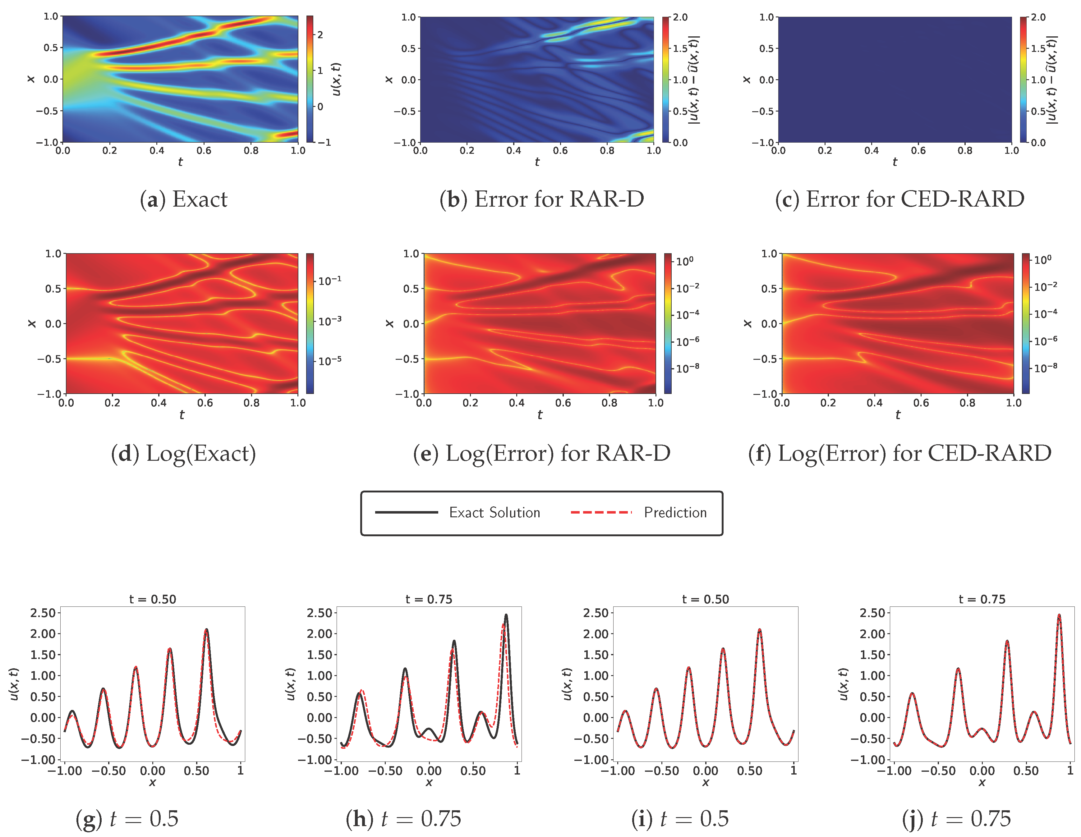
Here, u ( x , t ) is the velocity field and u ( t , x ; θ ) is the output from the neural network. To systematically increase the problem stiffness, we vary the kinematic viscosity ν from 0.02 / π to 0.005 / π . The surrogate model is constructed to satisfy both the initial condition and the hard constraints for the boundary conditions. For the Burgers’ equation-II, we analyze performance as the viscosity ν is reduced from 0.02 / π to 0.005 / π , which progressively increases problem difficulty. As shown in Table 5, the non-curriculum methods (Vanilla, RAR-G, RAR-D) and the CE-Vanilla baseline all fail catastrophically as viscosity decreases, with errors expanding by orders of magnitude and becoming unacceptably large. Notably, CE-Vanilla’s final error is even higher than that of the standard Vanilla PINN, indicating that a simple curriculum is insufficient for this problem. Notice that the curriculum-enhanced adaptive methods demonstrate far greater stability. Among them, CED-RARD is the clear standout, consistently achieving the lowest error across all viscosity levels. At the most challenging setting ( ν = 0.005 / π ), CED-RARD’s error of 1.69 × 10 2 is approximately 2.6 times lower than the next-best method (CE-RARD) and more than 22 times lower than CE-Vanilla, showcasing its superior robustness. Figure 5 provides a striking visual confirmation of these results by comparing the performance of CED-RARD against the non-curriculum RAR-D method at the lowest viscosity, ν = 0.005 / π . The absolute error plots (Figure 5b,c) reveal a dramatic difference: RAR-D suffers from massive, widespread error along the shockwave trajectories, while CED-RARD’s error is orders of magnitude smaller and almost negligible in comparison. This disparity is further emphasized in the time-slice plots (Figure 5d–g). The RAR-D predictions (Figure 5d,e) completely fail to capture the sharp “sawtooth” structure of the exact solution. In contrast, the CED-RARD predictions (Figure 5f,g) align almost perfectly with the exact solution, demonstrating exceptional fidelity in resolving the steep gradients. This visual evidence definitely confirms that the combination of curriculum learning and residual-informed distribution sampling in CED-RARD is critical for accurately solving this highly challenging problem where other methods completely break down.

3.6. Korteweg–De Vries Equation

We now address the Korteweg–de Vries (KdV) equation, a model for wave phenomena that balances nonlinear advection with third-order dispersion. The specific formulation we consider is given by:
u t + λ 1 u u x + λ 2 3 u x 3 = 0 , x [ 1 , 1 ] , t [ 0 , 1 ] IC : u ( 0 , x ) = cos ( π x ) BC : u ( t , 1 ) = u ( t , 1 ) , u x ( t , 1 ) = u x ( t , 1 )
In our experiments, we vary the nonlinear coefficient λ 1 in the range [ 1.0 , 2.5 ] , while the dispersive coefficient λ 2 is held fixed at 0.0025 . The surrogate solution, designed to enforce the initial condition, is defined as:
Surrogate : u ^ ( t , x ) = cos ( π x ) + t u ( t , x ; θ )
where u ( t , x ; θ ) is the output of the neural network. For the KdV equation, we evaluate the performance as the nonlinear coefficient λ 1 increases from 1.0 to 2.5, creating a more challenging problem with highly oscillatory solutions. As documented in Table 6, this proves catastrophic for the non-curriculum methods (Vanilla, RAR-G, RAR-D) and the CE-Vanilla baseline. All of these methods fail dramatically at λ 1 = 2.5 , with errors increasing by two to three orders of magnitude. In contrast, all four curriculum-enhanced adaptive methods remain exceptionally stable, with final errors below 10 2 . Among this group, CED-RARD demonstrates superior performance, consistently maintaining the lowest error and achieving a final error of just 3.7 × 10 3 . This is nearly twice as effective as the next-best methods (CE-RARD and CED-RARG) and over 100 times more accurate than the failed CE-Vanilla, highlighting the power of combining a difficulty-aware curriculum with residual-based distribution sampling. Figure 6 visually corroborates these findings by comparing the top-performing CED-RARD against the failed RAR-D method at the most difficult setting, λ 1 = 2.5 . The contrast is dramatic. The error plot for RAR-D (Figure 6b) shows massive, widespread error across the entire spatio-temporal domain, whereas the error for CED-RARD (Figure 6c) is virtually non-existent. The time-slice comparisons further underscore this point. The RAR-D predictions (Figure 6d,e) completely fail to capture the complex, multi-peak structure of the solution, exhibiting severe amplitude and phase errors. Conversely, the CED-RARD predictions (Figure 6f,g) are nearly indistinguishable from the exact solution, perfectly resolving the sharp peaks and oscillatory behavior. This visual evidence confirms that CED-RARD’s sophisticated sampling strategy is essential for achieving high-fidelity solutions for the highly nonlinear and oscillatory KdV equation, a regime where simpler methods completely break down.

3.7. Reaction Equation

The Reaction equation isolates nonlinear dynamics without diffusion, a property useful for modeling chemical kinetics or population growth, and is formally defined as follows:
u t ρ u ( 1 u ) = 0 , x [ 0 , 2 π ] , t [ 0 , 1 ]
IC : u ( x , 0 ) = exp ( x π ) 2 2 ( π / 4 ) 2 BC : u ( 0 , t ) = u ( 2 π , t ) Surrogate : u ^ ( t , x ) = exp ( x π ) 2 2 ( π / 4 ) 2 + t u ( t , x ; θ )
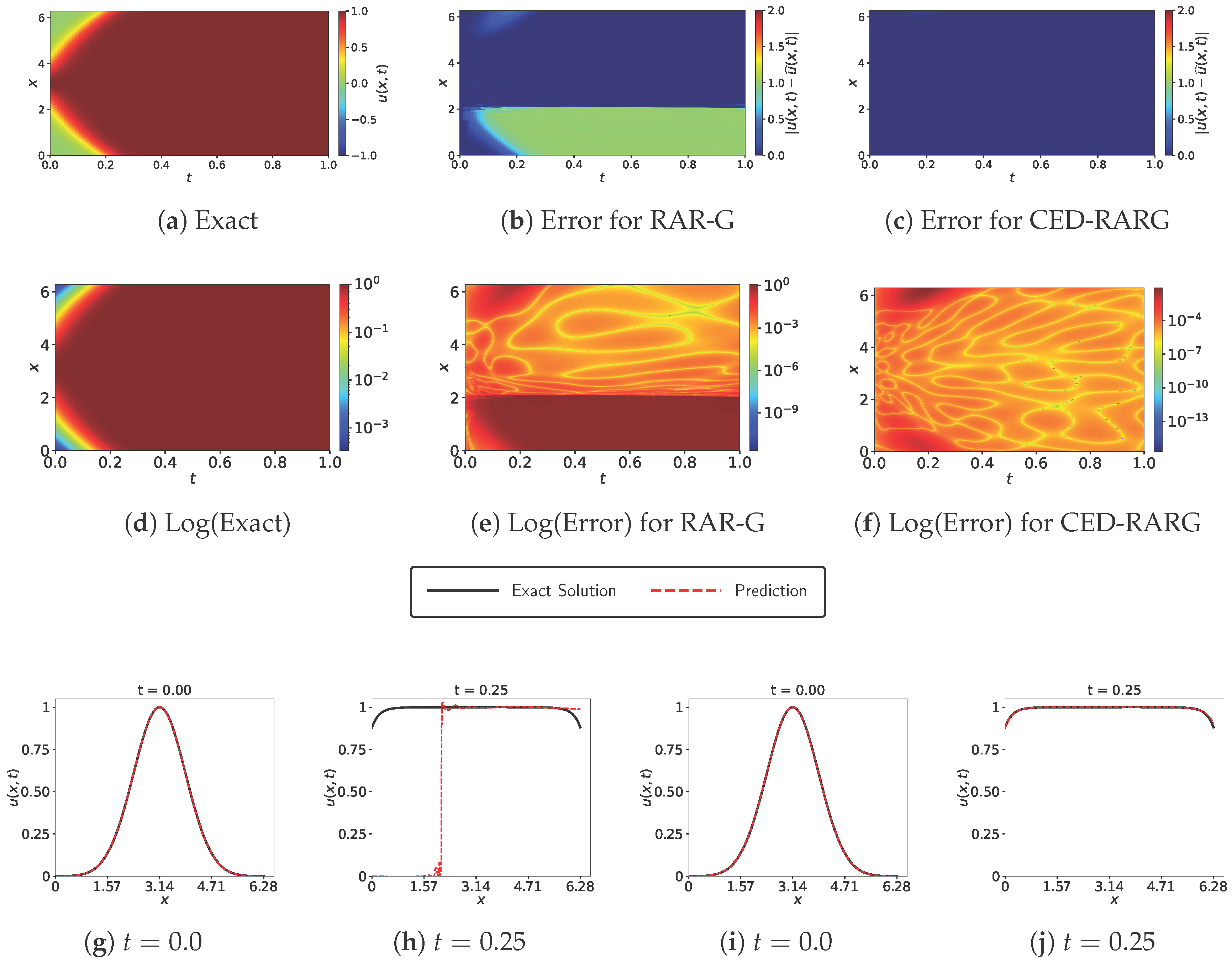
where ρ governs the reaction rate.For the Reaction equation, we analyze performance by increasing the reaction rate parameter ρ from 15 to 50. As shown in Table 7, increasing stiffness proves catastrophic for the non-curriculum methods (Vanilla, RAR-G, RAR-D), which all fail dramatically at ρ 40 with errors increasing by two orders of magnitude. However, all curriculum-based methods demonstrate exceptional stability. Even the simple CE-Vanilla maintains a low and stable error across the entire parameter range. However, the proposed adaptive methods achieve even greater accuracy. CED-RARG emerges as the top-performing method, securing the lowest error at the most challenging stage ( ρ = 50 ) with a value of 2.5 × 10 3 . This result is more than twice as accurate as CE-Vanilla and over 300 times more accurate than the failed Vanilla PINN, highlighting the significant benefit of combining a curriculum with difficulty-aware adaptive sampling. Figure 7 offers a striking visual confirmation of these results, comparing the successful CED-RARG against the failed RAR-G at the critical parameter ρ = 40 . The absolute error plots (Figure 7b,c) show a striking difference: RAR-G exhibits massive error concentrated along the reaction front, while the error for CED-RARG is nearly non-existent across the entire domain. This failure is further detailed in the time slices. At t = 0.25 (Figure 7e), the RAR-G prediction is completely incorrect, generating a sharp, unphysical step-like function instead of the smooth, diffused reaction front. In contrast, the CED-RARG prediction at the same time slice (Figure 7g) is visually indistinguishable from the exact solution. This analysis definitely demonstrates that while a simple curriculum can prevent failure in this problem, the advanced sampling strategy of CED-RARG is essential for achieving high-fidelity solutions that accurately capture the underlying physics of the reaction process.

4. Discussion and Conclusions

In this work, we introduced and evaluated four algorithms designed to improve PINNs in stiff PDEs by combining curriculum learning with adaptive sampling. The baseline adaptive methods, CE-RARG and CE-RARD, augment the training set within each curriculum stage by selecting new points based on a greedy refinement or a residual-informed distribution, respectively. Our proposed difficulty-aware variants, CED-RARG and CED-RARD, enhance this process by dynamically adjusting the number of refinement loops based on the relative difficulty between curriculum stages, thereby concentrating computational effort where it is most needed.
We evaluated these methods on five challenging PDE problems: the Allen–Cahn, Burgers’ (I and II), Korteweg–de Vries (KdV), and Reaction equations, each in highly stiff or nonlinear regimes. The results absolutely demonstrate that the curriculum-enhanced adaptive methods consistently and dramatically outperform baseline PINNs and non-adaptive curriculum learning (CE-Vanilla). Across all five test cases, the difficulty-aware variants, CED-RARG and CED-RARD, delivered state-of-the-art performance. For the Allen–Cahn and Reaction equations, CED-RARG proved most effective, reducing error by over 40% compared to its non-dynamic counterpart at the highest stiffness. For the Burgers’-I, Burgers’-II, and KdV equations, CED-RARD was the undisputed top performer, achieving final errors that were orders of magnitude lower than the baselines and significantly better than all other adaptive methods.
Despite these notable improvements, our analysis highlights that solving problems with extremely sharp gradients remains a challenge. In the Burgers’ equation at ν = 0.003 / π , even the best-performing CED-RARD exhibits minor deviations near the shock front, indicating that fully resolving such features is difficult (see Figure 4). This suggests that while our methods significantly raise the bar for PINN performance, extreme stiffness can still push the limits of the network’s expressive capacity. Overcoming this may require complementary techniques, such as increasing the density of collocation points, using gradient-based weighting, or designing new adaptive sampling strategies optimized for high-stiffness regimes.
These findings point to several promising directions for future work. First, integrating adaptive activation functions [4,35,36] with curriculum stages could allow the model to dynamically adjust its expressiveness in response to changing stiffness profiles. Second, hybrid training schemes that couple PINNs with classical numerical solvers, particularly during challenging curriculum transitions, may help stabilize convergence. Third, sequence-to-sequence frameworks could be enhanced to train a single, unified model that solves for a continuous range of stiffness parameters. This would enforce temporal causality while simultaneously learning a more generalized solution operator, making the model robust across different physical regimes. Finally, extending the proposed framework to more complex scenarios, such as coupled PDE systems or high-dimensional problems via domain decomposition, would enhance its practical utility. These advancements are essential for closing the performance gap between PINNs and conventional solvers in large-scale, stiff PDE settings.

Author Contributions

Conceptualization, H.C. and E.S.; Methodology, H.C. and F.A.; Software, H.C. and F.A.; Validation, H.C.; Investigation, H.C. and F.A.; Resources, H.C.; Data curation, H.C. and F.A.; Writing—original draft, H.C.; Writing—review & editing, H.C., F.A., M.T., H.N., M.N.N., H.K. and E.S.; Supervision, H.N., M.N.N. and E.S.; Project administration, E.S.; Funding acquisition, E.S. All authors have read and agreed to the published version of the manuscript.

Funding

This research received no external funding.

Data Availability Statement

The data presented in this study are openly available at CE-PINN, https://github.com/cetinkayahasan/CE-PiNN (accessed on 30 October 2025).

Acknowledgments

This work was supported by the TAMUQ Research Initiative. All experiments, implementation code, and MATLAB scripts for generating reference datasets are publicly available at https://github.com/cetinkayahasan/CE-PiNN (accessed on 30 October 2025). The authors declare that they have no conflict of interest. While preparing this work, the authors used OpenAI’s ChatGPT (GPT-4.1) to help fix spelling, grammar, clarity, and overall editing of their sentences. After using this tool, the authors carefully checked and updated the content as needed. The authors take full responsibility for everything included in this publication.

Conflicts of Interest

The authors declare no conflicts of interest.

References

  1. LeCun, Y.; Bengio, Y.; Hinton, G. Deep learning. Nature 2015, 521, 436–444. [Google Scholar] [CrossRef] [PubMed]
  2. Angermueller, C.; Pärnamaa, T.; Parts, L.; Stegle, O. Deep learning for computational biology. Mol. Syst. Biol. 2016, 12, 878. [Google Scholar] [CrossRef] [PubMed]
  3. Raissi, M.; Perdikaris, P.; Karniadakis, G.E. Physics-informed neural networks: A deep learning framework for solving forward and inverse problems involving nonlinear partial differential equations. J. Comput. Phys. 2019, 378, 686–707. [Google Scholar] [CrossRef]
  4. Cuomo, S.; Di Cola, V.S.; Giampaolo, F.; Rozza, G.; Raissi, M.; Piccialli, F. Scientific Machine Learning Through Physics–Informed Neural Networks: Where We Are and What’s Next. J. Sci. Comput. 2022, 92, 88. [Google Scholar] [CrossRef]
  5. Karniadakis, G.E.; Kevrekidis, I.G.; Lu, L.; Perdikaris, P.; Wang, S.; Yang, L. Physics-informed machine learning. Nat. Rev. Phys. 2021, 3, 422–440. [Google Scholar] [CrossRef]
  6. Raissi, M.; Yazdani, A.; Karniadakis, G.E. Hidden fluid mechanics: Learning velocity and pressure fields from flow visualizations. Science 2020, 367, 1026–1030. [Google Scholar] [CrossRef] [PubMed]
  7. Zhang, E.; Dao, M.; Karniadakis, G.E.; Suresh, S. Analyses of internal structures and defects in materials using physics-informed neural networks. Sci. Adv. 2022, 8, eabk0644. [Google Scholar] [CrossRef] [PubMed]
  8. Sahli Costabal, F.; Yang, Y.; Perdikaris, P.; Hurtado, D.E.; Kuhl, E. Physics-Informed Neural Networks for Cardiac Activation Mapping. Front. Phys. 2020, 8, 42. [Google Scholar] [CrossRef]
  9. Kurth, T.; Subramanian, S.; Harrington, P.; Pathak, J.; Mardani, M.; Hall, D.; Miele, A.; Kashinath, K.; Anandkumar, A. FourCastNet: Accelerating Global High-Resolution Weather Forecasting Using Adaptive Fourier Neural Operators. In Proceedings of the Platform for Advanced Scientific Computing Conference, Davos, Switzerland, 26–28 June 2023; ACM: New York, NY, USA, 2023. [Google Scholar]
  10. Baydin, A.G.; Pearlmutter, B.A.; Radul, A.A.; Siskind, J.M. Automatic Differentiation in Machine Learning: A Survey. J. Mach. Learn. Res. 2018, 18, 1–43. [Google Scholar]
  11. Paszke, A.; Gross, S.; Chintala, S.; Chanan, G.; Yang, E.; DeVito, Z.; Lin, Z.; Desmaison, A.; Antiga, L.; Lerer, A. Automatic differentiation in PyTorch. In NIPS 2017 Workshop on Autodiff; NIPS: Long Beach, CA, USA, 2017. [Google Scholar]
  12. Wang, S.; Teng, Y.; Perdikaris, P. Understanding and Mitigating Gradient Flow Pathologies in Physics-Informed Neural Networks. SIAM J. Sci. Comput. 2021, 43, A3055–A3081. [Google Scholar] [CrossRef]
  13. Wang, S.; Sankaran, S.; Perdikaris, P. Respecting causality for training physics-informed neural networks. Comput. Methods Appl. Mech. Eng. 2024, 421, 116813. [Google Scholar] [CrossRef]
  14. Tancik, M.; Srinivasan, P.; Mildenhall, B.; Fridovich-Keil, S.; Raghavan, N.; Singhal, U.; Ramamoorthi, R.; Barron, J.; Ng, R. Fourier Features Let Networks Learn High Frequency Functions in Low Dimensional Domains. In Advances in Neural Information Processing Systems 33; Curran Associates, Inc.: Red Hook, NY, USA, 2020; pp. 7537–7547. [Google Scholar]
  15. Sitzmann, V.; Martel, J.N.P.; Bergman, A.W.; Lindell, D.B.; Wetzstein, G. Implicit Neural Representations with Periodic Activation Functions. In Advances in Neural Information Processing Systems 33; Curran Associates, Inc.: Red Hook, NY, USA, 2020; pp. 7462–7473. [Google Scholar]
  16. McClenny, L.D.; Braga-Neto, U.M. Self-adaptive physics-informed neural networks. J. Comput. Phys. 2023, 474, 111722. [Google Scholar] [CrossRef]
  17. Krishnapriyan, A.; Gholami, A.; Zhe, S.; Kirby, R.; Mahoney, M.W. Characterizing possible failure modes in physics-informed neural networks. In Advances in Neural Information Processing Systems 34; Curran Associates, Inc.: Red Hook, NY, USA, 2021; pp. 26548–26560. [Google Scholar]
  18. Sikora, M.; Krukowski, P.; Paszyńska, A.; Paszyński, M. Comparison of Physics Informed Neural Networks and Finite Element Method Solvers for advection-dominated diffusion problems. J. Comput. Sci. 2024, 81, 102340. [Google Scholar] [CrossRef]
  19. Jagtap, A.D.; Karniadakis, G.E. Extended Physics-Informed Neural Networks (XPINNs): A Generalized Space-Time Domain Decomposition Based Deep Learning Framework for Nonlinear Partial Differential Equations. Commun. Comput. Phys. 2020, 28, 2002–2041. [Google Scholar] [CrossRef]
  20. Yu, J.; Lu, L.; Meng, X.; Karniadakis, G.E. Gradient-enhanced physics-informed neural networks for forward and inverse PDE problems. Comput. Methods Appl. Mech. Eng. 2022, 393, 114823. [Google Scholar] [CrossRef]
  21. Liu, L.; Liu, S.; Xie, H.; Xiong, F.; Yu, T.; Xiao, M.; Liu, L.; Yong, H. Discontinuity Computing Using Physics-Informed Neural Networks. J. Sci. Comput. 2023, 98, 22. [Google Scholar] [CrossRef]
  22. Toloubidokhti, M.; Ye, Y.; Missel, R.; Jiang, X.; Kumar, N.; Shrestha, R.; Wang, L. DATS: Difficulty-Aware Task Sampler for Meta-Learning Physics-Informed Neural Networks. In Proceedings of the Twelfth International Conference on Learning Representations, Vienna, Austria, 7–11 May 2024. [Google Scholar]
  23. Byrd, R.H.; Lu, P.; Nocedal, J.; Zhu, C. A Limited Memory Algorithm for Bound Constrained Optimization. SIAM J. Sci. Comput. 1995, 16, 1190–1208. [Google Scholar] [CrossRef]
  24. Wang, S.; Sankaran, S.; Wang, H.; Perdikaris, P. An Expert’s Guide to Training Physics-informed Neural Networks. arXiv 2023, arXiv:2308.08468. [Google Scholar]
  25. Bengio, Y.; Louradour, J.; Collobert, R.; Weston, J. Curriculum learning. In Proceedings of the 26th Annual International Conference on Machine Learning, Montreal, QC, Canada, 14–18 June 2009; Association for Computing Machinery: New York, NY, USA, 2009; pp. 41–48. [Google Scholar]
  26. Lu, L.; Meng, X.; Mao, Z.; Karniadakis, G.E. DeepXDE: A Deep Learning Library for Solving Differential Equations. SIAM Rev. 2021, 63, 208–228. [Google Scholar] [CrossRef]
  27. Wu, C.; Zhu, M.; Tan, Q.; Kartha, Y.; Lu, L. A comprehensive study of non-adaptive and residual-based adaptive sampling for physics-informed neural networks. Comput. Methods Appl. Mech. Eng. 2023, 403, 115671. [Google Scholar] [CrossRef]
  28. Tang, K.; Wan, X.; Yang, C. DAS-PINNs: A deep adaptive sampling method for solving high-dimensional partial differential equations. J. Comput. Phys. 2023, 476, 111868. [Google Scholar] [CrossRef]
  29. Nabian, M.A.; Gladstone, R.J.; Meidani, H. Efficient training of physics-informed neural networks via importance sampling. Comput.-Aided Civ. Infrastruct. Eng. 2021, 36, 962–977. [Google Scholar] [CrossRef]
  30. Gao, W.; Wang, C. Active learning based sampling for high-dimensional nonlinear partial differential equations. J. Comput. Phys. 2023, 475, 111848. [Google Scholar] [CrossRef]
  31. Daw, A.; Bu, J.; Wang, S.; Perdikaris, P.; Karpatne, A. Rethinking the Importance of Sampling in Physics-Informed Neural Networks. arXiv 2022, arXiv:2207.02338. [Google Scholar]
  32. Glorot, X.; Bengio, Y. Understanding the difficulty of training deep feedforward neural networks. In Proceedings of the Thirteenth International Conference on Artificial Intelligence and Statistics, PMLR, Sardinia, Italy, 13–15 May 2010; Volume 9, pp. 249–256. [Google Scholar]
  33. Kingma, D.P.; Ba, J. Adam: A Method for Stochastic Optimization. In Proceedings of the 3rd International Conference on Learning Representations, ICLR 2015, San Diego, CA, USA, 7–9 May 2015. [Google Scholar]
  34. Driscoll, T.A.; Hale, N.; Trefethen, L.N. (Eds.) Chebfun Guide; Pafnuty Publications: Oxford, UK, 2014. [Google Scholar]
  35. Wang, H.; Lu, L.; Song, S.; Huang, G. Learning Specialized Activation Functions for Physics-Informed Neural Networks. Commun. Comput. Phys. 2023, 34, 869–906. [Google Scholar] [CrossRef]
  36. Roy, S.; Annavarapu, C.; Roy, P.; Sarma, K.A.K. Adaptive Interface-PINNs (AdaI-PINNs): An Efficient Physics-Informed Neural Networks Framework for Interface Problems. Commun. Comput. Phys. 2025, 37, 603–622. [Google Scholar] [CrossRef]
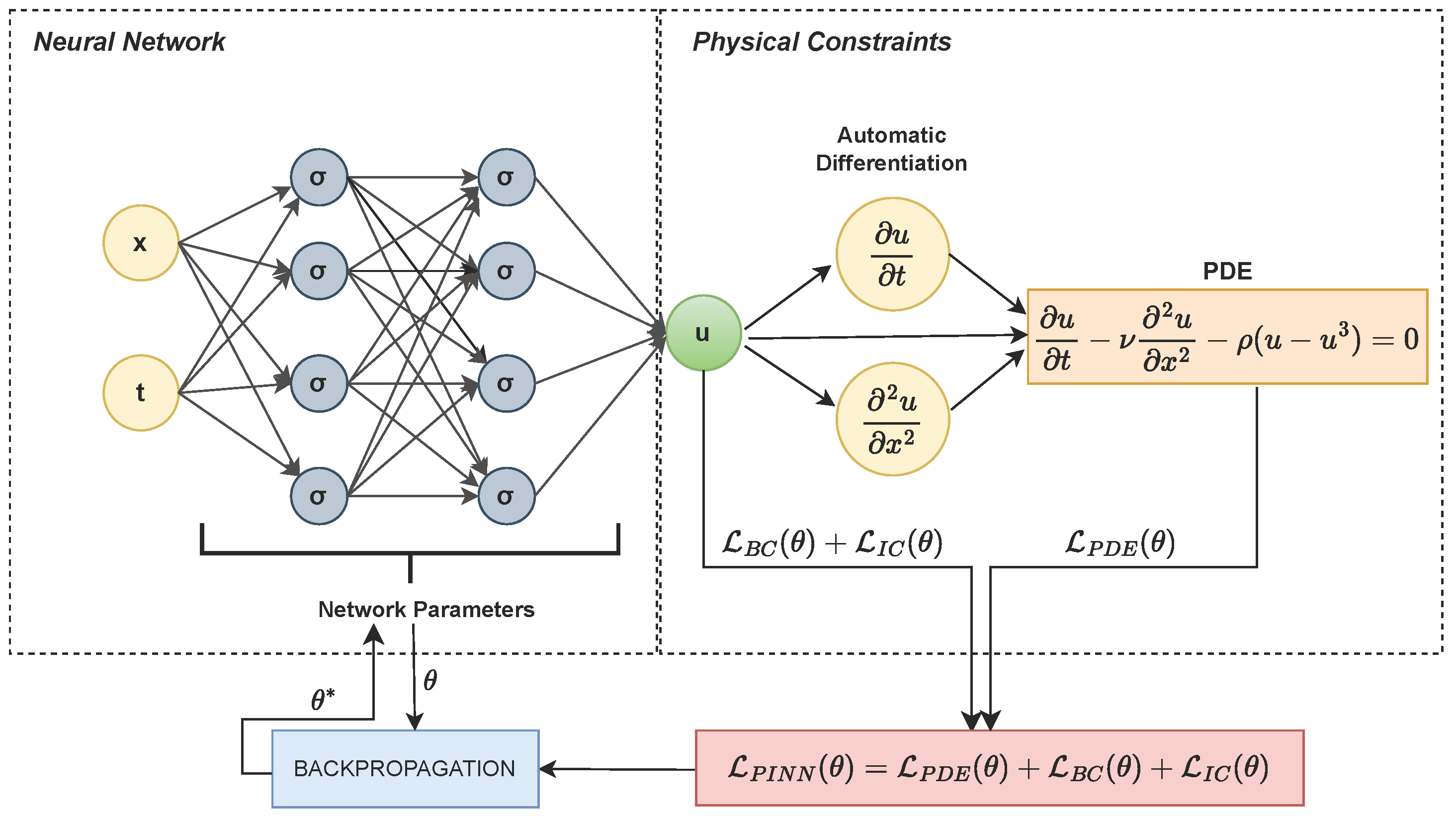
Figure 1. Overview of PINN framework. The neural network maps spatial and temporal inputs ( x , t ) to the solution u, which is used to compute the residual of the governing PDE via automatic differentiation. The total loss L PINN ( θ ) consists of the PDE residual loss L PDE ( θ ) , boundary condition loss L BC ( θ ) , and initial condition loss L IC ( θ ) . These losses are minimized jointly through backpropagation to optimize the network parameters θ .
Mathematics 13 03996 g001
Figure 2. Comparison of the CE-Vanilla and CED-RARG methods on the Allen–Cahn equation with diffusion coefficient D = 0.001 and reaction rate ρ = 10 . The panels show: (a) The exact solution. (b) Absolute error for CE-Vanilla. (c) Absolute error for CED-RARG. (d) Logarithm of the exact solution. (e) Logarithm of the absolute error for CE-Vanilla. (f) Logarithm of the absolute error for CED-RARG. (g) Solution slice for CE-Vanilla at t = 0.5 . (h) Solution slice for CE-Vanilla at t = 0.75 . (i) Solution slice for CED-RARG at t = 0.5 . (j) Solution slice for CED-RARG at t = 0.75 .
Mathematics 13 03996 g002
Figure 3. Comparison of the RAR-G and CED-RARG methods on the AC equation with nonlinear coefficient ρ = 8 where RARG/RARD both methods fail. The panels show: (a) The exact solution. (b) Absolute error for RAR-G. (c) Absolute error for CED-RARG. (d) Logarithm of the exact solution. (e) Logarithm of the absolute error for RAR-G. (f) Logarithm of the absolute error for CED-RARG. (g) Solution slice for RAR-G at t = 0.5 . (h) Solution slice for RAR-G at t = 0.75 . (i) Solution slice for CED-RARG at t = 0.5 . (j) Solution slice for CED-RARG at t = 0.75 .
Mathematics 13 03996 g003
Figure 4. Comparison of the CE-Vanilla and CED-RARD methods on the Burgers’ equation-I with viscosity ν = 0.003 / π . The panels show: (a) The exact solution. (b) Absolute error for CE-Vanilla. (c) Absolute error for CED-RARD. (d) Logarithm of the exact solution. (e) Logarithm of the absolute error for CE-Vanilla. (f) Logarithm of the absolute error for CED-RARD. (g) Solution slice for CE-Vanilla at t = 0.5 . (h) Solution slice for CE-Vanilla at t = 0.75 . (i) Solution slice for CED-RARD at t = 0.5 . (j) Solution slice for CED-RARD at t = 0.75 .
Mathematics 13 03996 g004
Figure 5. Comparison of the RAR-D and CED-RARD methods on the Burgers’ equation-II with viscosity ν = 0.005 / π . The panels show: (a) The exact solution. (b) Absolute error for RAR-D. (c) Absolute error for CED-RARD. (d) Logarithm of the exact solution. (e) Logarithm of the absolute error for RAR-D. (f) Logarithm of the absolute error for CED-RARD. (g) Solution slice for RAR-D at t = 0.5 . (h) Solution slice for RAR-D at t = 0.75 . (i) Solution slice for CED-RARD at t = 0.5 . (j) Solution slice for CED-RARD at t = 0.75 .
Mathematics 13 03996 g005
Figure 6. Comparison of the RAR-D and CED-RARD methods on the KdV equation with nonlinear coefficient λ 1 = 2.5 . The panels show: (a) The exact solution. (b) Absolute error for RAR-D. (c) Absolute error for CED-RARD. (d) Logarithm of the exact solution. (e) Logarithm of the absolute error for RAR-D. (f) Logarithm of the absolute error for CED-RARD. (g) Solution slice for RAR-D at t = 0.5 . (h) Solution slice for RAR-D at t = 0.75 . (i) Solution slice for CED-RARD at t = 0.5 . (j) Solution slice for CED-RARD at t = 0.75 .
Mathematics 13 03996 g006
Figure 7. Comparison of the RAR-G and CED-RARG methods on the Reaction equation with nonlinear coefficient ρ = 40 where RAR-G/RAR-D methods fail first. The panels show: (a) The exact solution. (b) Absolute error for RAR-G. (c) Absolute error for CED-RARG. (d) Logarithm of the exact solution. (e) Logarithm of the absolute error for RAR-G. (f) Logarithm of the absolute error for CED-RARG. (g) Solution slice for RAR-G at t = 0.0 . (h) Solution slice for RAR-G at t = 0.25 . (i) Solution slice for CED-RARG at t = 0.0 . (j) Solution slice for CED-RARG at t = 0.25 .
Mathematics 13 03996 g007
Table 1. Relative L 2 errors for the Allen–Cahn equation with diffusion coefficient D = 0.001 , evaluated across varying values of the parameter.
Method ρ = 5 ρ = 6 ρ = 7 ρ = 8 ρ = 9 ρ = 10
Vanilla0.00750.02370.64510.67980.72290.7187
CE-Vanilla0.00120.00760.01290.01510.02240.0244
RAR-G0.00640.00870.00620.66780.66730.7518
CE-RARG0.00090.00130.00360.00540.00770.0080
CED-RARG0.00060.00140.00810.00570.00500.0046
RAR-D0.00530.01210.03670.64510.69160.7126
CE-RARD0.00100.00380.01650.03660.03740.0379
CED-RARD0.00100.00310.00650.00980.00720.0082
Table 2. Ablation study on computational cost vs. accuracy for the Allen–Cahn equation at the final curriculum stage ( ρ = 10 ).
MethodFinal Rel. L2 ErrorTotal LoopsTotal Points AddedTraining Time
CE-RARG0.0080300 (fixed)∼75001.0× (baseline)
CED-RARG0.0046∼500 (dynamic)∼12,500∼1.3×
Table 3. Relative L 2 errors for the Allen–Cahn equation with diffusion coefficient D = 0.001 , evaluated for the parameter ρ = 10 . The reported mean and standard deviation are computed over 30 independent runs to assess stability and robustness.
Method ρ = 10
Vanilla 0.7185 ± 4.54 × 10 2
CE-Vanilla 0.0249 ± 3.53 × 10 3
RAR-G 0.7314 ± 1.55 × 10 2
CE-RARG 0.0081 ± 5.07 × 10 4
CED-RARG 0.0045 ± 2.86 × 10 4
RAR-D 0.7128 ± 5.89 × 10 3
CE-RARD 0.0375 ± 1.24 × 10 3
CED-RARD 0.0079 ± 8.86 × 10 4
Table 4. Relative L 2 errors for the Burgers’ equation-I for different values of the viscosity parameter.
Method ν = 0.009 π ν = 0.008 π ν = 0.007 π ν = 0.006 π ν = 0.005 π ν = 0.003 π
Vanilla0.00040.09510.03940.36830.41980.5101
CE-Vanilla0.00860.016660.02480.03690.01250.1578
RAR-G0.00030.00050.00070.00120.00040.1048
CE-RARG0.00020.00040.00060.00090.00180.0086
CED-RARG0.00040.00040.00060.00110.00190.0045
RAR-D0.00010.00030.00040.00110.00040.1339
CE-RARD0.00040.00040.00070.00110.00240.0078
CED-RARD0.00020.00020.00030.00040.00080.0023
Table 5. Relative L 2 errors for the Burgers’ equation-II for different values of the viscosity parameter.
Method ν = 0.02 π ν = 0.01 π ν = 0.009 π ν = 0.008 π ν = 0.007 π ν = 0.005 π
Vanilla0.03940.15160.16600.16520.34510.3173
CE-Vanilla0.00970.05840.07680.28890.33560.3798
RAR-G0.00040.00060.00890.04780.08090.1703
CE-RARG0.00020.00440.00560.00960.01320.0603
CED-RARG0.00030.00370.01190.00970.02570.0558
RAR-D0.00030.01230.00900.07540.14430.1302
CE-RARD0.00030.00260.00440.00680.01040.0447
CED-RARD0.00020.00100.00210.00310.00500.0169
Table 6. Relative L 2 errors for the KdV equation with fixed λ 2 = 0.0025 , evaluated across varying values of the parameter λ 1 . The CE-Vanilla loss is used to assess task difficulty due to its more stable residual distribution.
Method λ 1 = 1.0 λ 1 = 1.3 λ 1 = 1.5 λ 1 = 1.7 λ 1 = 2.0 λ 1 = 2.5
Vanilla0.00140.00280.02680.31920.74831.0589
CE-Vanilla0.00080.00130.00200.00340.00610.3777
RAR-G0.00080.00190.00290.00580.04470.4207
CE-RARG0.00080.00110.00210.00250.00280.0081
CED-RARG0.00080.00120.00180.00200.00220.0069
RAR-D0.00170.00150.00270.00570.01460.3221
CE-RARD0.00070.00120.00210.00240.00230.0064
CED-RARD0.00060.00110.00160.00240.00230.0037
Table 7. Relative L 2 errors for the Reaction equation across different values of the reaction rate parameter ρ .
Method ρ = 15 ρ = 20 ρ = 25 ρ = 30 ρ = 40 ρ = 50
Vanilla0.00690.00940.01220.05460.56920.8305
CE-Vanilla0.00810.00710.00690.00710.00610.0054
RAR-G0.00570.02710.00300.00400.56190.6232
CE-RARG0.00440.00550.00400.00270.00290.0027
CED-RARG0.00150.00470.00270.00310.00300.0025
RAR-D0.00690.00860.00760.00440.62820.6474
CE-RARD0.00620.00700.00730.00610.00400.0032
CED-RARD0.00150.00680.00640.00400.00360.0030
Disclaimer/Publisher’s Note: The statements, opinions and data contained in all publications are solely those of the individual author(s) and contributor(s) and not of MDPI and/or the editor(s). MDPI and/or the editor(s) disclaim responsibility for any injury to people or property resulting from any ideas, methods, instructions or products referred to in the content.