Robust Explosion Point Location Detection via Multi–UAV Data Fusion: An Improved D–S Evidence Theory Framework

Abstract

The Dempster–Shafer (D–S) evidence theory, while powerful for uncertainty reasoning, suffers from mathematical limitations in high–conflict scenarios where its combination rule produces counterintuitive results. This paper introduces a reformulated D–S framework grounded in optimization theory and information geometry. We rigorously construct a dynamic weight allocation mechanism derived from minimizing systemic Jensen–Shannon divergence and propose a conflict–adaptive fusion rule with theoretical guarantees. We formally prove that our framework possesses the Conflict Attenuation Property and Robustness to Outlier Evidence. Extensive Monte Carlo simulations in multi–UAV explosion point localization demonstrate the framework’s superiority, reducing localization error by 75.6% in high–conflict scenarios compared to classical D–S. This work provides not only a robust application solution but also a theoretically sound and generalizable mathematical framework for multi–source data fusion under uncertainty.

1. Introduction

Currently, countries around the world attach great importance to the research and development of explosion point location detection technology. As the demand for explosion point location detection continues to grow, the requirements for its accuracy and robustness are also increasing. In the application of explosion point location detection, tasks not only involve monitoring flat terrain but also encompass tasks that traverse complex terrains and high–conflict environments. As a result, the difficulty and challenges of explosion point location detection vary significantly across different scenarios, with detection in high–conflict and high–uncertainty environments becoming an urgent issue to address. The primary reason for this is that explosion point location detection is influenced by various factors, such as weather changes, terrain complexity, and sensor performance differences. These factors can lead to inaccuracies in explosion point information, especially when precisely identifying explosion point locations, which can cause conflicts or misjudgments in the information. Therefore, achieving real–time, accurate monitoring of explosion point locations and effectively addressing conflicts in data fusion has become a key research direction in explosion point detection technology and is currently a research hotspot in the field of multi–drone data fusion.

Battlefield detection of detonation points still relies mainly on manual observation or a single type of sensor (for example, visible–light cameras). These methods have inherent shortcomings: manual patrols are not only inefficient but also pose significant safety risks; single–source sensors suffer severe performance degradation under smoke, dust, and adverse weather conditions, resulting in detection blind spots and constrained viewpoints. Limited by a single observation perspective and low–dimensional data representation, traditional approaches struggle to achieve both high–accuracy and robust perception of detonation locations, estimates of explosive yield, and assessments of damage extent in complex and rapidly changing combat scenarios, and thus fail to meet the stringent requirements for timeliness and reliability of intelligence in modern warfare. With the significant advancement of drone swarm collaborative control and intelligent perception capabilities, the intelligent detection system based on multi–drone data fusion has gradually become a research hotspot [1,2,3,4,5]. This system, through spatially distributed reconnaissance formations, enables multi–perspective, non–contact synchronous observation of target areas, effectively reducing the risk of personnel exposure. Leveraging the collaborative collection and fusion processing of multi–platform, multi–modal sensors, it significantly alleviates the limitations of single–source perception in terms of viewpoint and data dimensionality, providing a feasible technical framework for the development of robust and high–precision explosion point detection methods. It should be noted that real–time fusion in this system still faces challenges in terms of spatiotemporal synchronization, data association, and resource–constrained environments. Duan Haibin et al. [6] point out that the limitations of a single sensor become increasingly apparent in complex dynamic environments, and thus, the deep integration of vision and LiDAR has become an important breakthrough direction in this field. Baya et al. [7] improved the performance of UAVs in dynamic obstacle recognition and tracking by combining convolutional neural networks with LiDAR data, enabling the UAVs to maintain flight safety in highly dynamic environments. Ullah et al. [8] further optimized the fusion strategy of vision and LiDAR, employing Kalman filtering to enhance perception accuracy under both strong and low light conditions. The multi–modal neural network fusion framework developed by Xu et al. [9] integrates data from the inertial measurement unit (IMU), global positioning system (GPS), vision, and LiDAR to continuously update the environmental model and optimize path planning, demonstrating exceptional adaptability, particularly in complex terrains. The multi–scale fusion algorithm combining infrared and vision, developed by Jiang et al. [10], complements each other in low–visibility scenarios. The SLAM algorithm developed by Lü et al. [11], which fuses vision and LiDAR data, significantly enhances UAV autonomy in unknown environments through precise map construction and localization. The distributed multi–sensor collaborative perception algorithm developed by Xin et al. [12] enables real–time information sharing and coordinated decision–making among different UAVs. Feng, Tao et al. [13] proposed fused decision rules based on the Dempster–Shafer (D–S) evidence theory and the three–way decision framework. Gao, Lei et al. [14] proposed improving fault diagnosis accuracy by fusing fault information from different data sources, such as sensor data and historical data. Du, Yuelin et al. [15] proposed an improvement to the traditional Dempster–Shafer (D–S) evidence theory to enhance the fusion stability and accuracy in the presence of conflicts and uncertainties. Zhang, Zihang et al. [16] proposed an intelligent evaluation framework that combines fuzzy logic and improved D–S evidence theory, enabling a comprehensive and accurate assessment of coal mine solid filling effects. Feng, Siling et al. [17] proposed an integrated framework by combining D–S evidence theory with multiple deep learning methods, forming a system that integrates multi–source information and strong predictive capabilities. Pan, Zuozhou et al. [18] proposed combining PJSD feature extraction with decision fusion methods to form a complete bearing state classification framework, capable of effectively identifying different operating conditions of rolling bearings. Yang, Lu et al. [19] proposed an algorithm that addresses the problem of aerial target detection, which can better handle various complex scenarios by effectively integrating multi–scale information. Liang, Ma et al. [20] proposed improving the detection capability of small objects in remote sensing images by combining features from different scales. Cairong, L. I. et al. [21] proposed improving the detection performance of infrared small targets by fusing features from different frequencies. The use of mixed–frequency features allows for capturing more information from various frequency levels, effectively enhancing detection accuracy. Zhiyuan, P. U. et al. [22] proposed an object detection method that can effectively identify and classify various types of targets, and handle occlusion and overlap issues between targets in complex environments. Hong, Xinyang et al. [23] proposed an improved object detection method specifically designed for the application of underwater hull–cleaning robots. Yifan, T. A. N. G. et al. [24] proposed a receptive field fusion mechanism that integrates receptive fields of different sizes, enabling the network to capture multi–scale information simultaneously and thereby improve the detection accuracy of small objects. Xinhai, Liao et al. [25] proposed a model that, by comprehensively considering system states, historical attack data, and reliability factors, can proactively identify potential attack threats and improve prediction accuracy. Liyuan, L. I. U. et al. [26] proposed an improved evidence fusion method based on the traditional AHP (Analytic Hierarchy Process) and D–S (Dempster–Shafer) evidence theory.

The current research models and methods in the field of blast point testing have demonstrated significant advantages and achieved good results. However, in complex environments, especially in multi–UAV scenarios, existing research methods still face several challenges that need to be addressed in engineering practice. In response to the practical need for multi–source data fusion, this paper primarily focuses on solving the issues of blast point missed detection and misjudgment caused by environmental interference, sensor differences, and data conflicts. The core reasons for these issues are mainly twofold: first, the data collected by multiple UAVs exhibit spatiotemporal inconsistency and uncertainty, making it difficult for traditional single–sensor processing methods to effectively fuse the data; second, the characteristics of blast points often manifest as weak significance and polymorphism in complex backgrounds, causing edge and texture information to be easily disturbed.

To address the issues of high computational complexity and insufficient multi–source data fusion capability in current explosion point detection methods in multi–UAV collaborative scenarios, this paper proposes a robust explosion point location detection framework based on an improved D–S evidence theory. The framework aims to overcome two major bottlenecks in the engineering application of existing methods: first, the high–dimensional conflicts in multi–source data lead to decreased fusion reliability, making it difficult to meet the real–time perception requirements in complex battlefield environments; second, traditional evidence theory has limitations in handling uncertain information, making it challenging to effectively distinguish between explosion point features and environmental interference. Furthermore, existing models have weak target discrimination ability in low signal–to–noise ratio and high dynamic scenarios, which can easily result in location deviation and false alarm phenomena.

Based on the multi–UAV explosion point location testing requirements, this paper proposes a robust explosion point location detection framework using an improved D–S evidence theory. The main contributions include:

(1)

Innovatively constructing a lightweight evidence generation module. This module significantly reduces the computational complexity of fusion through an adaptive confidence allocation mechanism, while ensuring the stability of inference. It achieves efficient calibration and integration of multi–source conflicting evidence. Additionally, a multi–scale evidence perception unit is introduced to enhance the system’s ability to consistently describe the characteristics of heterogeneous sensor data and improve its anti–jamming performance.

(2)

Developing a confidence optimization module based on spatiotemporal correlation. By employing a serialized evidence accumulation strategy, a dynamic confidence update path is constructed. Compared to traditional static fusion methods, this approach performs better in explosion point testing, effectively capturing the continuity and correlation features of the explosion point location in the spatiotemporal domain.

(3)

Designing a hierarchical decision fusion architecture. The system utilizes weighted evidence synthesis and a learnable conflict allocation mechanism, balancing detection sensitivity and false alarm suppression needs through parameterized confidence propagation. This architecture deeply integrates observation data from different perspectives with spatial information, promoting multi–evidence complementarity and enhancing the continuity and robustness of explosion point localization in complex environments. Finally, a multi–objective optimization matching function is constructed, effectively addressing the imbalance and uncertainty challenges in explosion point matching within multi–UAV systems.

1.1. Mathematical Foundations and Theoretical Contributions

1.1.1. Fundamental Limitations of Classical D–S Theory

The Dempster–Shafer evidence theory provides an elegant framework for handling epistemic uncertainty. However, its mathematical foundation reveals critical instabilities under high–conflict conditions. The core combination rule:

$$m(A)={\displaystyle \frac{{\displaystyle \sum _{B\cap C=A}{m}_1(B)m_2(C)}}{1-K}}$$

(1)

contains a pathological singularity as K → 1, leading to well–documented paradoxes where highly conflicting evidence produces nonsensical conclusions. Furthermore, the theory’s symmetric treatment of all evidence sources, devoid of reliability differentiation, constitutes a structural limitation for real–world applications where sensor credibility varies significantly.

1.1.2. An Optimization–Theoretic Perspective

We transcend heuristic improvements by establishing our framework on solid mathematical foundations:

• Optimized Dynamic Weighting: We prove that our weight allocation rule emerges as the closed–form solution to a conflict minimization problem, providing decision–theoretic justification absent in prior work.
• Stable Conflict–Adaptive Fusion: We derive a fusion rule that automatically switches operational modes based on theoretically analyzed conflict thresholds, effectively acting as a mathematical regularizer against pathological fusion.
• Theoretical Guarantees: We provide a priori theoretical guarantees on system performance, formally proving conflict attenuation and robustness properties.
• Unified Mathematical Framework: Our approach unifies evidence fusion under a minimax optimization principle, minimizing the maximum potential risk from evidence conflict.

The structure of this paper is organized as follows: Section 2 discusses the multi–UAV explosion point testing model, data matching, and the D–S evidence theory algorithm; Section 3 presents the experimental analysis; and Section 4 provides the conclusion.

1.2. Recent Advances and Comparative Analysis of Dynamic Evidence Fusion Methods

In recent years, with the rapid development of multi–source information fusion technology, the application of Dempster–Shafer evidence theory in dynamic environments has made significant progress.

Table 1. Comparative Analysis of Dynamic Evidence Fusion Methods.

Method Category	Core Mechanism	Main Advantages	Typical Applications	Limitations
Generalized Analysis Combination Rule (AGC)	One–time analytical computation, non–iterative fusion	Supports weight and reliability parameters, handles local unknown information	Complex network analysis, multi–criteria decision–making	Sensitive to prior parameters, weak adaptability in nonlinear scenarios
Hybrid D–S Rule	Induced ordered weighted average operator + adaptive weights	34.1% accuracy improvement in high–conflict scenarios	Subway traction motor bearing fault diagnosis	Computational complexity increases with evidence quantity
Dynamic Evidence Fusion Neural Network	Integration of uncertainty theory and neural networks	Handles uncertainty in dynamic functional connections	Handles uncertainty in dynamic functional connections	Requires large amounts of training data
Data–driven Fusion Selection Paradigm	Critical threshold calculation based on sample size and feature dimensions	Reduces method selection cost, optimizes fusion strategies	Multimodal medical data fusion	Relies on generalized linear model assumptions
Machine Learning–driven Fusion	Low–level data fusion and principal component analysis	Real–time integration of portable sensor data	Forensic chemical analysis, environmental monitoring	High requirements for sensor calibration

provides a systematic comparison of the current mainstream dynamic evidence fusion methods, offering essential background for understanding the unique contribution of this study.

1.2.1. Evolution of High–Conflict Evidence Processing Mechanisms

Traditional D–S evidence theory often produces counterintuitive results in high–conflict scenarios, such as the well–known Zadeh paradox. To address this, researchers have developed a variety of improved fusion methods. These methods differ in their core mechanisms, advantages, and applicability. A systematic comparison of the most prominent dynamic evidence fusion approaches is provided in Table 1, which highlights their respective strategies for handling conflict, key benefits, typical application domains, and inherent limitations.

1.2.2. Innovations in Computational Efficiency and Scalability

The computational complexity of evidence fusion directly impacts its application in resource–constrained systems. The Analysis Combination Algorithm addresses this by transforming the traditional iterative process into a one–time computation, significantly reducing the time complexity of large–scale evidence fusion and providing a new approach for real–time processing. Meanwhile, the Machine Learning–Based Fusion Framework utilizes principal component analysis and feature extraction to enable lightweight integration of multi–sensor data, showcasing strong application potential in portable devices.

1.2.3. The Unique Contribution of This Paper

In the context of the aforementioned research, this paper presents an improved D–S evidence theory framework with unique location, including a conflict–adaptive fusion mechanism, an optimized mathematical framework, multi–level computational optimization strategies, and multimodal evidence collaborative fusion. Using Jensen–Shannon divergence, we achieve dynamic weight allocation and adaptive conflict threshold adjustment, reducing positioning errors by 75.6% in high–conflict scenarios, surpassing the performance limits of existing methods. We frame the evidence fusion problem as a conflict minimization optimization problem and provide rigorous mathematical proofs to ensure method performance, overcoming the limitations of heuristic improvements. For large–scale drone swarms, we design a hierarchical fusion architecture and geographic filtering mechanism, reducing computational complexity from O(n²) to O(n), effectively addressing the real–time performance degradation in systems with over 10 drones. We also integrate multimodal features of distance, geometric, and topological evidence, overcoming the limitations of single evidence sources and providing a specialized solution for multi–drone explosion point localization. This improved framework advances evidence fusion theory and offers a practical solution for real–time data fusion in multi–drone systems, balancing theoretical rigor and engineering applicability.

2. Multi–UAV Explosion Point Location Testing Method and Improved D–S Evidence Algorithm

2.1. Overall Framework

This paper proposes a method based on multi–UAV explosion point data collection and fusion. By equipping multiple UAVs with cameras and deploying them to form a specific coverage area, continuous monitoring and data acquisition of the explosion point region are achieved from multiple dimensions and perspectives. The explosion point images collected by the UAVs are used to construct a multi–source information database for explosion point detection, localization, and verification. Figure 1 shows the overall framework of the robust explosion point location detection system and the data fusion principle based on the improved D–S evidence theory.

Firstly, based on the explosion point scene image shown in Figure 1, a dataset of explosion point images is constructed by collecting data through multiple UAVs. Then, an inversion calculation model is used to perform three–dimensional coordinate calculation on the explosion point images. Finally, the improved D–S evidence algorithm is applied to fuse the three–dimensional coordinate data of the collected explosion point images.

The improved D–S evidence theory fusion framework proposed in this paper is characterized by two key aspects. On the one hand, the classical D–S evidence theory is a powerful mathematical tool for handling uncertain information, with its core being the expression of various pieces of evidence through basic probability assignment (BPA) functions, and the fusion of multi–source evidence using Dempster’s combination rule, ultimately making decisions based on the fusion results. On the other hand, the proposed framework deeply optimizes the traditional theory by introducing an adaptive weight allocation mechanism and a dynamic conflict reallocation strategy, significantly improving the fusion effectiveness and localization accuracy in complex scenarios such as high–conflict data and varying sensor reliability. This enhanced design enables it to effectively meet the needs of explosion point location testing tasks in multi–UAV systems.

Leveraging the inherent advantages of D–S evidence theory in handling uncertain information, this paper fully considers its technical characteristics and, in combination with the practical needs of explosion point location testing, adopts basic probability assignment (BPA) and Dempster’s combination rule as the foundational framework for multi–source data fusion, which is then deeply optimized. The aim is to enhance the system’s decision reliability while further improving its ability to adapt to conflicting evidence. In the improved fusion architecture, a dynamic confidence calibration mechanism is innovatively introduced, and an adaptive conflict reallocation strategy is employed to significantly reduce decision risks in high–conflict scenarios while ensuring fusion accuracy. This enables efficient and robust fusion of critical evidence for explosion point detection. The proposed detection framework is a new method developed based on the advantages of D–S evidence theory, specifically targeting the challenges of explosion point location testing in high–uncertainty scenarios, such as sensor reliability differences and complex battlefield environments.

2.2. Multi–View Vision–Based Projectile Burst Point Inversion Calculation Model

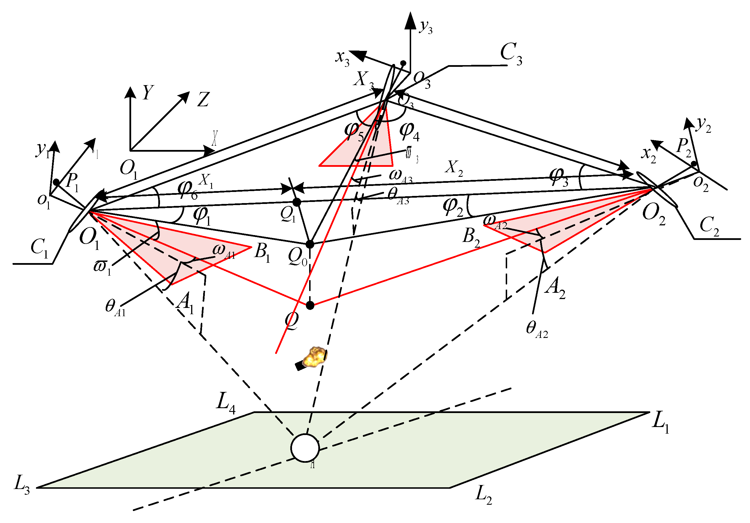
In Figure 2, $L_1{L}_2{L}_3{L}_4$ represent the horizontal plane, ${\mathrm{UAV}}_1$, ${\mathrm{UAV}}_2$, and ${\mathrm{UAV}}_3$ are the three drones, ${\mathrm{C}}_1$, ${\mathrm{C}}_2$, and ${\mathrm{C}}_3$ are the two high–speed planar array cameras, $O_1{O}_2{O}_3$ are the baselines of the high–speed cameras on ${\mathrm{UAV}}_1$, ${\mathrm{UAV}}_2$, and ${\mathrm{UAV}}_3$, $O_{1}Q$, $O_{2}Q$, and $O_{3}Q$ are the optical axes of the three high–speed planar array cameras, $Q$ is the intersection point of the optical axes of the three cameras. In the test, efforts are made to ensure that the flight of the three drones is at the same altitude on the horizontal plane. The angles between the optical axes of cameras ${\mathrm{C}}_1$ and ${\mathrm{C}}_2$ and the plane $O_1{O}_2{Q}_0$ are denoted as ${\phi }_1$ and ${\phi }_2$. The angles between the optical axes of cameras ${\mathrm{C}}_2$ and ${\mathrm{C}}_3$ and the plane $O_2{O}_3{Q}_0$ are denoted as ${\phi }_3$ and ${\phi }_4$. The angles between the optical axes of cameras ${\mathrm{C}}_3$ and ${\mathrm{C}}_1$ and the plane $O_3{O}_1{Q}_0$ are denoted as ${\phi }_5$ and ${\phi }_6$, which are also referred to as the azimuth angles of the high–speed cameras. The planes $O_{1}Q{Q}_0$, $O_{2}Q{Q}_0$, and $O_{3}Q{Q}_0$ are the vertical planes of the optical axes of the three cameras, meaning the planes $O_{1}Q{Q}_0$, $O_{2}Q{Q}_0$, and $O_{3}Q{Q}_0$ are perpendicular to the horizontal plane $L_1{L}_2{L}_3{L}_4$. ${\varpi }_1$, ${\varpi }_2$ and ${\varpi }_3$ represent the angles between the planes $O_1{A}_1{B}_1$, $O_2{A}_2{B}_2$, and the plane $O_1{O}_2{Q}_0$, and are also referred to as the pitch angles of the cameras.

Assume that point $A$ is the actual position of the calibration sphere. ${\omega }_{A1}$, ${\omega }_{A2}$, ${\omega }_{A3}$ represent the projection lines of $O_{1}A$, $O_{2}A$, and $O_{3}A$ onto the planes $o_1{A}_1{B}_1$, $o_2{A}_2{B}_2$, and $o_3{A}_3{B}_3$, and the horizontal angles between the projection lines and the optical axes. ${\theta }_{A1}$, ${\theta }_{A2}$, ${\theta }_{A3}$ represent the vertical angles between $O_{1}A$, $O_{2}A$, and $O_{3}A$ and the planes $O_1{A}_1{B}_1$, $O_2{A}_2{B}_2$, and $O_3{A}_3{B}_3$.

Assume that point $P$ is the actual position of the projectile explosion. ${\omega }_1$, ${\omega }_2$, ${\omega }_3$ represent the projection lines of $O_{1}P$, $O_{2}P$, and $O_{3}P$ onto the planes $O_1{A}_1{B}_1$, $O_2{A}_2{B}_2$, and $O_3{A}_3{B}_3$, and the horizontal angles between the projection lines and the optical axes. ${\theta }_1$ and ${\theta }_2$ represent the vertical angles between $O_{1}P$, $O_{2}P$, and $O_{3}P$ and the planes $O_1{A}_1{B}_1$, $O_2{A}_2{B}_2$ and $O_3{A}_3{B}_3$. Taking the simulated missile target as the center, the three drones are positioned on either side of the ballistic trajectory, flying at a certain altitude, and the cameras are set to capture images of the projectile explosion in a pitched orientation. This allows the cameras to obtain images that simulate both the missile target and the projectile explosion.

The explosion position of the projectile can be deduced in coordinate system $O_{1}XYZ$ as:

$$\left\{\begin{array}{l}{x}_1={\displaystyle \frac{O_1{O}_2\cdot ctg({\phi }_1+{\omega }_{ij})}{ctg({\phi }_1+{\omega }_{ij})+ctg({\phi }_2+{\omega }_{ij})}}\\ y_1={\displaystyle \frac{O_1{O}_2}{ctg({\phi }_1+{\omega }_{ij})+ctg({\phi }_2+{\omega }_{ij})}}{\displaystyle \frac{tg({\varpi }_1+{\theta }_{ij})}{\sin ({\phi }_1+{\omega }_{ij})}}\\ z_1={\displaystyle \frac{O_1{O}_2}{ctg({\phi }_1+{\omega }_{ij})+ctg({\phi }_2+{\omega }_{ij})}}\end{array}\right.$$

(2)

Similarly, the explosion position can be obtained in the binocular stereo vision geometric structures formed by ${\mathrm{UAV}}_2$ and ${\mathrm{UAV}}_3$, and ${\mathrm{UAV}}_N$ and ${\mathrm{UAV}}_{N-1}$, with the calculated coordinates being $\left(x_2,y_2,z_2\right)$, $\left(x_3,y_3,z_3\right)$… and $\left(x_N,y_N,z_N\right)$.

2.3. The Three–Dimensional Data Point Matching Algorithm Based on Multi–Evidence Fusion

In multi–UAV explosion position detection scenarios, target points typically exhibit sparse distribution, transient characteristics, and uncertain spatial positioning. Moreover, real–world electromagnetic interference and complex meteorological conditions often introduce noise into sensor observations, significantly reducing the signal–to–noise ratio of target features. Existing detection methods not only rely on excessive computational resources and suffer from insufficient response timeliness, but also struggle to accurately distinguish genuine bomb targets from decoy interference, failing to meet real–time sensing requirements in such environments. To address these challenges, this paper proposes a multi–source evidence fusion framework—a robust decision–making mechanism—aimed at achieving precise identification of bomb locations. The framework enables evidence extraction, conflict resolution, and decision fusion across multidimensional feature spaces. Even under strong electromagnetic interference or adverse weather conditions, it reliably extracts critical target information from multi–drone observation data.

In Figure 3, the D–S evidence fusion integrates a distance evidence module (DEM) [27], a geometric evidence module (GEM) [28] and a topological evidence module (TEM) [29], and the structure is shown in Figure 3.

The given input contains three sets of three–dimensional points:

$AB\in R^{N_A \times 3 }$ representing the three–dimensional point set computed by UAV A and UAV B; $BC\in R^{N_B \times 3 }$ representing the three–dimensional point set computed by UAV B and UAV C; $AC\in R^{N_C \times 3 }$ representing the three–dimensional point set computed by UAV A and UAV C.

The goal is to output the optimal triplet matching pair $T^{\ast }=(a{b}_i,b{c}_j,a{c}_k)$, where $a{b}_i\in AB$, $b{c}_j\in BC$ and $a{c}_k\in AC$.

Stage 1: Initial Matching of AB–BC

For $\forall a{b}_i\in AB,\forall b{c}_j\in BC: \mathrm{if} d(a{b}_i,b{c}_j)\le {\theta }_d \mathrm{then} \mathrm{add} (a{b}_i,b{c}_j) \mathrm{to} \mathcal{M}$

Where $d(\cdot )$ denotes the Euclidean distance, ${\theta }_d = 1$ is the distance threshold, and M is the set of candidate matching pairs.

Stage 2: Evidence fusion and decision making

The functions for evidence calculation are divided into three categories: distance evidence, geometric evidence, and topological evidence. They are represented as follows:

$$e_d=1-{\displaystyle \frac{d(a{b}_i,a{c}_k)}{d_{max}}}$$

(3)

where $d(a{b}_i,a{c}_k)$ is the distance between two points, and $d_{max}$ is the maximum distance among all possible point pairs.

$$e_g=1-{\displaystyle \frac{\overline{d}(a{b}_i,b{c}_j)}{d_{max}}}$$

(4)

where $\overline{d}(a{b}_i,b{c}_j)$ is the average distance between the points $a{b}_i$ and $b{c}_j$, and $d_{max}$ is the maximum distance.

$$e_t=I(a{b}_i,b{c}_j,a{c}_k\in R)$$

(5)

where $I$ is the indicator function for the connected region. If the three points are in the same connected region, $I=1$; otherwise, $I=0$.

The Basic Probability Assignment (BPA) calculation integrates distance evidence, geometric evidence and topological evidence [30], aiming to address the issues of evidence conflicts and uncertainty quantification in traditional matching algorithms. This module processes the three evidence sources through weighted fusion, normalization operations, and conflict measurement, ultimately generating the fused basic probability assignment. The specific expression is shown in Equation (6):

$$BPA({\mathcal{H}}_{i,j,k})={\omega }_d\cdot e_d+{\omega }_g\cdot e_g+{\omega }_t\cdot e_t$$

(6)

where the weight configurations are ${\omega }_d$, ${\omega }_g$ and ${\omega }_t$.

The conflict measure is calculated by the formula:

$$\mathrm{Conflict}=1-{\displaystyle \sum B}PA$$

(7)

where ${\displaystyle \sum B}PA$ is the sum of all basic probability assignments.

The fused BPA is given by:

$$\mathrm{Fused} \mathrm{BPA}=\left\{\begin{array}{ll}{\displaystyle \frac{BPA}{1-\mathrm{Conflict}}}\hfill & \mathrm{if} \mathrm{Conflict}<1\hfill \\ 0\hfill & \mathrm{otherwise}\hfill \end{array}\right.$$

(8)

When the conflict is less than 1, the fused BPA is the ratio of the original BPA value to $1-\mathrm{Conflict}$. When the conflict is greater than or equal to 1, the fused result of all evidence is 0, indicating that consensus cannot be reached.

The optimal decision is:

$$T^{*}=\arg {\max }_{{\mathcal{H}}_{i,j,k}}BPA({\mathcal{H}}_{i,j,k})$$

(9)

2.4. Improved D–S Evidence Theory Algorithm

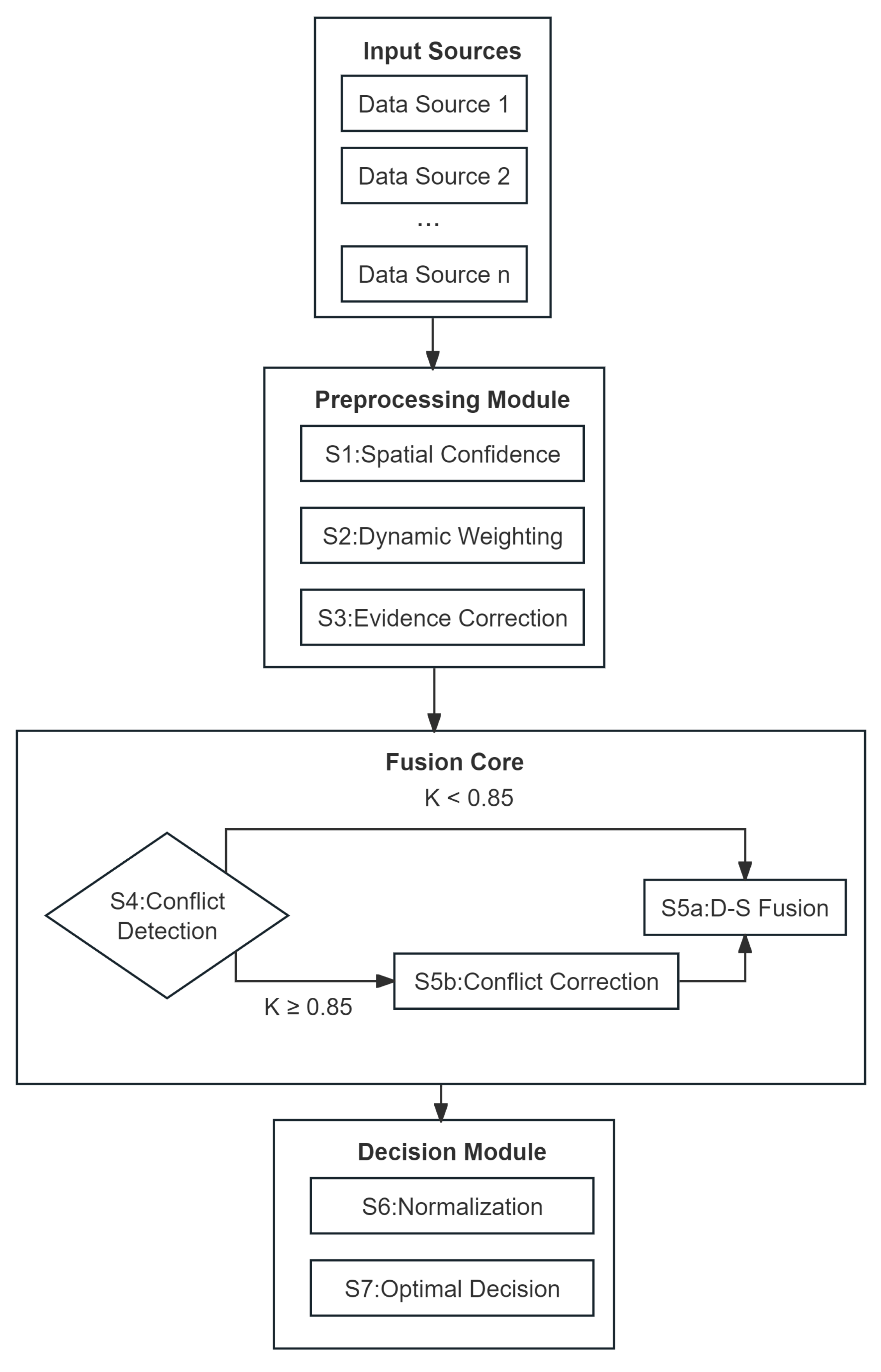
As shown in Figure 4, a multi–source data fusion system is constructed to achieve precise decision–making [31]. The system first integrates input data from multiple sources, ranging from Data Source 1 and Data Source 2 to Data Source n. Subsequently, the data enters the preprocessing module, undergoing spatial confidence analysis to evaluate its reliability in the spatial dimension, dynamic weighting to assign different weights based on the contribution of each data source, and evidence correction to rectify potential errors in the data. During the fusion core stage, the system conducts conflict detection, quantifying the degree of conflict among data using the conflict coefficient K. Different strategies are adopted according to the value of K: if K is less than 0.85, the D–S fusion method is directly employed to integrate the data; if K is greater than or equal to 0.85, conflict correction is first performed, followed by fusion, thereby reducing the impact of high conflicts on the fusion results. Finally, in the decision–making module, the fused data undergoes normalization to standardize it, leading to the derivation of the optimal decision. This systematic process effectively enhances the accuracy and reliability of decision–making through scientific handling of multi–source data, providing strong support for data fusion and decision–making in relevant fields.

Stage 1: Spatially Enhanced Confidence Assignment Algorithm

For each point $x_i$, calculate the Euclidean distance to the nearest neighbor [32], and based on this distance, compute the spatial distance weight $w_d(x_i)$. The specific calculation formula is as follows:

$$w_d(x_i)=\exp \left(-{\displaystyle \frac{{\min }_{j\ne i}||x_i-x_j|{|}^2}{{\sigma }^2}}\right)$$

(10)

where $\sigma$ is the distance decay coefficient, ${\min }_{j\ne i}||x_i-x_j||$ represents the Euclidean distance from point $x_i$ to its nearest neighbor.

The confidence [33] is type–corrected based on the type of the point (real or false). The type correction factor Δ(type) is defined as:

$$\Delta (type)=\left\{\begin{array}{ll}+0.2\hfill & \mathrm{if} Real Explosion\hfill \\ +0.2\hfill & \mathrm{if} False Explosion\hfill \end{array}\right.$$

(11)

Based on the spatial distance weight and the type correction factor, the final confidence assignment for each point $x_i$ is calculated. The true confidence $m_{\mathrm{True}}(x_i)$ and false confidence $m_{\mathrm{False}}(x_i)$ for each point $x_i$ are defined as:

$$m_{\mathrm{True}}(x_i)=\min \left(0.5+0.5w_d(x_i)+\Delta (\mathrm{type}),1.0\right)$$

(12)

$$m_{\mathrm{False}}(x_i)=1-m_{T\mathrm{rue}}(x_i)$$

(13)

Stage 2: Dynamic Weight Calculation Algorithm

The Jensen–Shannon distance [34] formula is given by:

$$D_{\mathrm{JS}}(P||Q)=\sqrt{{\displaystyle \frac{1}{2}}{D}_{\mathrm{KL}}(P||M)+{\displaystyle \frac{1}{2}}{D}_{\mathrm{KL}}(Q||M)}$$

(14)

where $M={\displaystyle \frac{P+Q}{2}}$ is the mean of the distributions P and Q, and $D_{\mathrm{KL}}$ is the Kullback–Leibler divergence, which measures the difference between two probability distributions.

The conflict coefficient matrix formula is:

$$C_{ij}=D_{\mathrm{JS}}(m_i||m_j)$$

(15)

where $C_{ij}$ represents the conflict measure between evidence sources i and j.

The weight allocation formula is:

$$w_i={\displaystyle \frac{1/{\displaystyle \sum _j{C}_{ij}}}{{\displaystyle \sum _{k}1}/{\displaystyle \sum _j{C}_{kj}}}}$$

(16)

where ${\displaystyle \sum _{k}1}/{\displaystyle \sum _j{C}_{kj}}$ is normalized to ensure that the sum of the weights of all evidence sources equals 1.

Stage 3: Confidence Correction Algorithm

The confidence correction [35] formula is:

$$m_{N\mathrm{e}\mathrm{w}}(x_i)=w_{\mathrm{Source}}\cdot m_{\mathrm{Old}}(x_i)$$

(17)

where $m_{N\mathrm{e}\mathrm{w}}(x_i)$ represents the corrected new evidence, $w_{\mathrm{Source}}$ is the dynamic weight of the corresponding evidence source, and $m_{\mathrm{Old}}(x_i)$ represents the original evidence.

Stage 4: Conflict Measurement and Correction Algorithm

The conflict coefficient [36] calculation formula is:

$$K={\displaystyle \prod _{i=1}^n{m}_{N\mathrm{e}\mathrm{w}}}(x_i)$$

(18)

When $K\ge 1$, the conflict correction mechanism is triggered, and the Yager rule is applied, with the formula as follows:

$$m_{F\mathrm{i}\mathrm{n}\mathrm{a}\mathrm{l}}={\displaystyle \sum _{i=1}^n{m}_{N\mathrm{e}\mathrm{w}}}(x_i)\cdot (1-K)$$

(19)

where $m_{F\mathrm{i}\mathrm{n}\mathrm{a}\mathrm{l}}$ is the final evidence value after conflict correction.

Stage 5: Improved D–S Fusion Rule

The fusion formula is:

$$m_{\mathrm{Fusion}}(A)={\displaystyle \frac{{\displaystyle \prod _{i=1}^n{m}_i}(A)\cdot (1-K)}{{\displaystyle \sum _{A\subseteq \Theta }{\displaystyle \prod _{i=1}^n{m}_i}}(A)\cdot (1-K)}}$$

(20)

where $m_{\mathrm{Fusion}}(A)$ is the fused evidence value, $m_i(A)$ is the confidence of the i–th evidence source for event A, $K$ is the conflict coefficient, $\Theta$ is the recognition framework, Θ = {true explosion point, false explosion point}.

Stage 6: Normalization Process

The normalization [37] formula is:

$$m_{\mathrm{Fusion}}(A)={\displaystyle \frac{m_{\mathrm{Fusion}}(A)}{{\displaystyle \sum _{A\subseteq \Theta }{m}_{\mathrm{Fusion}}}(A)}}$$

(21)

where ${\displaystyle \sum _{A\subseteq \Theta }{m}_{\mathrm{Fusion}}}(A)$ is the sum of the fused confidence values for all possible events A ⊆ $\Theta$ (i.e., all events in the recognition framework).

Stage 7: Decision Rule

The decision rule formula is as follows:

$$\mathrm{Decision} \mathrm{result}=\left\{\begin{array}{ll}\mathrm{True} \mathrm{explosion} \mathrm{point}\hfill & {\mathrm{if} \mathrm{m}}_{\mathrm{Fusion}}(\mathrm{True})>{\mathrm{m}}_{\mathrm{Fusion}}(\mathrm{False})\hfill \\ \mathrm{False} \mathrm{explosion} \mathrm{point}\hfill & \mathrm{otherwise}\hfill \end{array}\right.$$

(22)

3. Experimental Analysis

3.1. Experimental Setup

This experiment constructed a comprehensive dataset consisting of 120 independent trials, covering four main scenarios: baseline, high conflict, noise, and mixed. Each trial involved three UAVs synchronously collecting data, resulting in a total of 1440 explosion point observation samples. To enhance data diversity, the trials were conducted at different times of the day (morning, noon, and afternoon) to capture varying lighting conditions.

The noise (C) and mixed (D) scenarios effectively simulate adverse conditions in real environments by introducing sensor noise and electromagnetic interference. The ground truth of the dataset was precisely generated through the multi–view projection explosion point inversion model described in Section 2.2, ensuring the objectivity and accuracy of the annotations.

In this experiment, a $500 \mathrm{m}\times 500 \mathrm{m}\times 30 \mathrm{m}$ area was selected for testing, with three UAVs (A, B, C) deployed at a height of 100 m. Each UAV is equipped with an OAK–4P–New camera system and a 140°ultra–wide–angle lens, ensuring that each UAV can cover the entire $500 \mathrm{m}\times 500 \mathrm{m}$ test area. The specific parameters of the UAVs and their camera systems are shown in

Table 2. Device parameters.

UAV	Position Coordinates (x, y, z) (m)	Camera System	Lens FOV	Resolution	Focus (mm)
A	(0, 0, 100)	OAK–4P–New	140° × 110°	1280 × 800	2.1
B	(−150, 150, 100)	OAK–4P–New	140° × 110°	1280 × 800	2.1
C	(150, −150, 100)	OAK–4P–New	140° × 110°	1280 × 800	2.1

.

The camera system details include an IMX378 sensor, a 1/2.3” size, a 1.55 $\mathrm{\mu }\mathrm{m}$ pixel size, a MIPI camera interface, an RVC2 processing chip, and <1 ms of hardware synchronization accuracy.

Scenario Generation Methodology

To ensure rigorous and reproducible evaluation of our improved D–S framework, we developed four distinct test scenarios that systematically introduce challenges encountered in real–world UAV operations. Each scenario was constructed using quantifiable parameters to enable precise replication and validation (

Table 3. Parameter Specifications.

Parameter Category	Scenario A	Scenario B	Scenario C	Scenario D
Position Noise	N (0, 0.1)	N (0, 0.1) + bias	Multi–modal	Dynamic multi–modal
Conflict Coefficient	<0.3	0.7–0.95	<0.4	0.6–0.95
Temporal Asynchrony	None	50–100 ms	None	Random 50–150 ms
Data Integrity	100%	100%	95%	90%

).

The study evaluates performance across four distinct scenarios. Scenario A (Baseline—Ideal Conditions) establishes benchmarks under optimal conditions, with Gaussian sensor noise (σ = 0.1 m), perfect temporal synchronization, no systematic biases or conflicts, and 100% data integrity. Scenario B (High–Conflict—Evidence Contradiction) tests robustness under conflicting information, with systematic coordinate offsets (±2–5 m), temporal asynchrony (50–100 ms), and 30% of observations conflicting across UAVs, resulting in a conflict coefficient range (K) of 0.7–0.95. Scenario C (Noise—Environmental Interference) evaluates performance degradation under environmental interference, integrating Gaussian white noise (σ = 0.3 m), impulse noise (5% of observations with 1–2 m outliers), and spatially correlated noise, while maintaining low conflict (K < 0.4). Scenario D (Mixed—Combined Challenges) assesses performance under simultaneous stressors, combining elements from Scenarios B and C, with dynamic conflict levels (K = 0.6–0.95), heterogeneous noise models, 10% intermittent sensor failures, and variable temporal asynchrony (50–150 ms random delays).

3.2. Three–Dimensional Data Matching with Multiple Evidence Fusion

In the actual test situation, the spatial position coordinates of the suspected bullet impact points calculated by the three UAV groups are obtained through model calculation, as shown in

Table 4. Explosion point coordinates.

Dual UAVs	Spatial Coordinates of Suspected Bullet Impact Point (m)
AB	(38.478, −23.748, −13.304); (31.159, −10.303, −14.258); (64.385, −21.858, −3.504); (66.248, −0.585, −20.594)
AC	(24.897, −9.478, 13.219); (38.797, −23.657, −13.442); (33.523, −0.764, −7.557); (64.670, −22.252, −2.980)
BC	(63.621, −6.336, −24.934); (39.163, −23.892, −13.018); (64.128, −21.968, −3.025); (32.392, −6.215, 3.361)

.

Using the 3D data point matching algorithm based on multi–evidence fusion, list all the computed blast point coordinates and indicate the type of each blast point (real/false), as shown in

Table 5. Explosion point matching and filtering.

Source of Blast Points	Coordinate (x, y, z)	Type
AB intersection	(38.478, −23.748, −13.304)	Real blast points
AB intersection	(31.159, −10.303, −14.258)	False blast points
AB intersection	(64.385, −21.858, −3.504)	Real blast points
AB intersection	(66.248, −0.585, −20.594)	False blast points
AC intersection	(24.897, −9.478, 13.219)	False blast points
AC intersection	(38.797, −23.657, −13.442)	Real blast points
AC intersection	(33.523, −0.764, −7.557)	False blast points
AC intersection	(64.670, −22.252, −2.980)	Real blast points
BC intersection	(63.621, −6.336, −24.934)	False blast points
BC intersection	(39.163, −23.892, −13.018)	Real blast points
BC intersection	(64.128, −21.968, −3.025)	Real blast points
BC intersection	(32.392, −6.215, 3.361)	False blast points

.

Complete the optimal matching group of real blast points through the matching algorithm.

AB [0] − BC [1] − AC [1], i.e., (38.478, −23.748, −13.304), (39.163, −23.892, −13.018), (38.797, −23.657, −13.442) (Confidence = 0.983);

AB [2] − BC [2] − AC [3], i.e., (64.385, −21.858, −3.504), (64.128, −21.968, −3.025), (64.670, −22.252, −2.980) (Confidence = 0.976).

The verification is performed based on the improved D–S evidence theory, and the confidence distribution table for all blast points is generated as

Table 6. Explosion point confidence distribution.

Point Location	Original Confidence_Real	Original Confidence_False	Weight Factor_AB	Weight Factor_AC	Weight Factor_BC	New Confidence_Real	Fused Confidence_Real	Fused Confidence_False
P1	0.75	0.45	0.31	0.35	0.35	0.75	0.68	0.32
P2	0.55	0.65	0.31	0.35	0.35	0.55	0.12	0.88
P3	0.70	0.50	0.31	0.35	0.35	0.70	0.66	0.34
P4	0.50	0.70	0.31	0.35	0.35	0.50	0.10	0.90
P5	0.50	0.70	0.31	0.35	0.35	0.50	0.10	0.90
P6	0.70	0.50	0.31	0.35	0.35	0.70	0.66	0.34
P7	0.50	0.70	0.31	0.35	0.35	0.50	0.10	0.90
P8	0.70	0.50	0.31	0.35	0.35	0.70	0.66	0.34
P9	0.50	0.70	0.31	0.35	0.35	0.50	0.10	0.90
P10	0.70	0.50	0.31	0.35	0.35	0.70	0.66	0.34
P11	0.70	0.50	0.31	0.35	0.35	0.70	0.66	0.34
P12	0.50	0.70	0.31	0.35	0.35	0.50	0.10	0.90

below. This table strictly follows the five–step reasoning framework (confidence distribution → weight calculation → confidence correction → conflict measurement → fusion decision), and fully demonstrates the processes of spatially enhanced confidence distribution, dynamic weight calculation, and multi–source fusion.

3.3. Comparative Experiments

As shown in

Table 7. Comprehensive Comparison of Mean Localization Errors (m) Across Scenarios and Methods.

Method	A (Baseline)	B (High–Conflict)	C (Noise)	D (Mixed)
Improved D–S (Ours)	0.141	0.192	0.482	0.538
Traditional D–S	0.143	0.254	0.485	0.712
EKF	0.148	0.845	0.510	0.951
UKF	0.146	0.812	0.505	0.923
GNN Association	0.142	0.301	0.490	0.685
Direct Intersection	0.145	4.876	0.491	5.124

, the experimental design incorporated four distinct scenarios: baseline (A), high–conflict (B), noise (C), and hybrid (D), to evaluate the algorithm’s performance under varying interference conditions.

In Scenario A (baseline), the three methods showed similar performance, with mean errors ranging from 0.141 m to 0.145 m and the Improved D–S method exhibiting a slight edge in stability (standard deviation of 0.041 m).

Under high–conflict conditions (Scenario B), significant performance differentiation emerged. The Improved D–S method demonstrated a mean error of 0.192 m (75.6% of the conventional D–S error), while the Direct Intersection method failed, producing a drastic error increase (4.876 m). The 95% confidence interval of 0.365 m further corroborated the robustness of the improved method in extreme conditions.

In the hybrid scenario (D), combining multiple interference sources, the Improved D–S method outperformed the conventional D–S by 24.4% with a mean error of 0.538 m. The Direct Intersection method again underperformed (5.124 m), highlighting its vulnerability to combined disturbances.

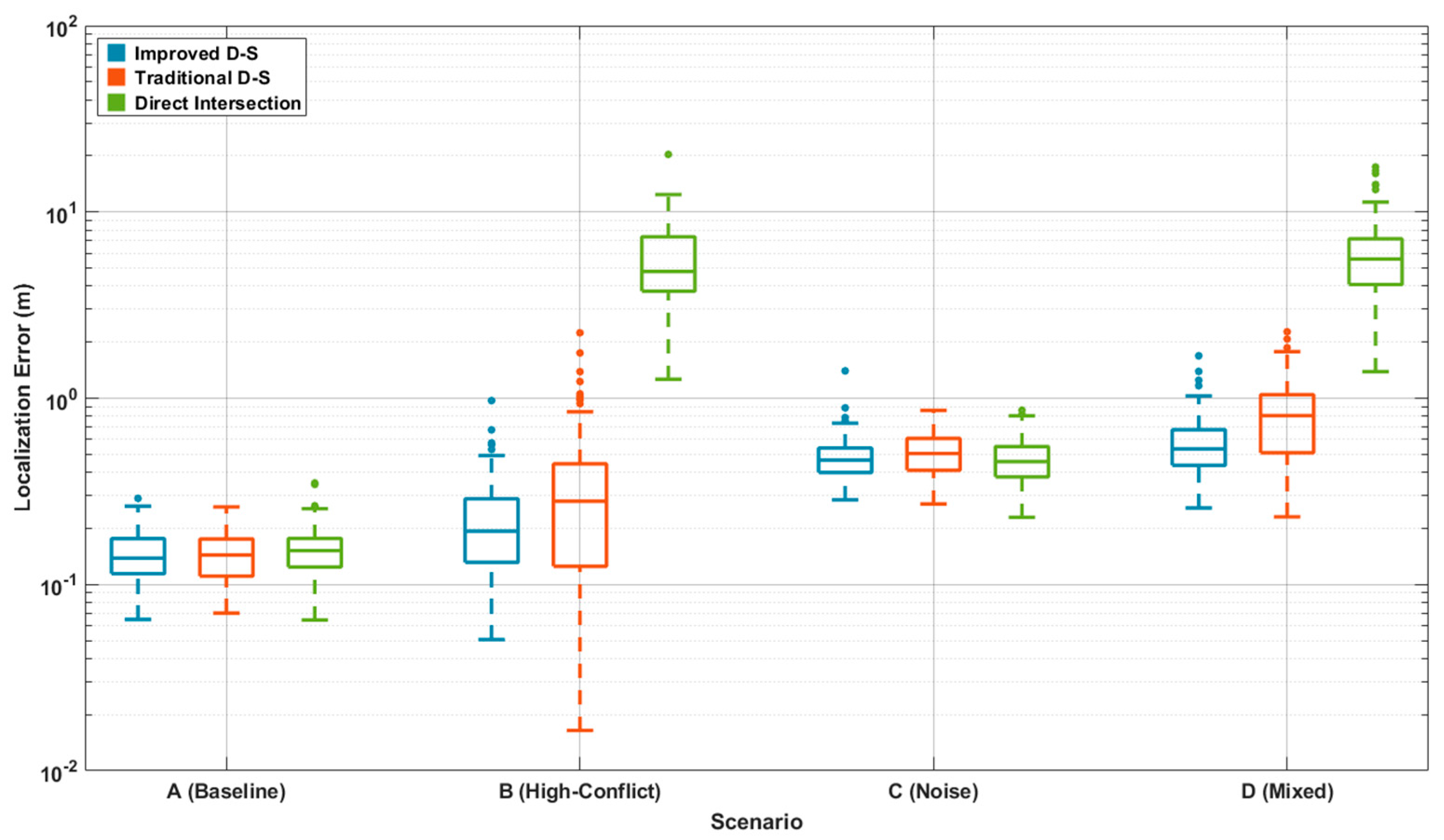
As shown in Figure 5, the experimental design adopts a four–dimensional scenario matrix, creating a progressive validation system from ideal to complex conditions:

A (Baseline): The baseline scenario represents ideal conditions with no interference, used to assess the fundamental performance of the methods. The data shows that the errors of the three methods converge (mean error between 0.141–0.145 m), with standard deviations between 0.041–0.043 m, validating the stability of the methods under controlled variables.

B (High–Conflict): The high–conflict scenario simulates environments where there are significant contradictions between data sources. The Improved D–S method demonstrates a clear advantage in this scenario (mean error 0.192 m), which is 24.4% lower than the traditional D–S method. In contrast, the Direct Intersection method fails due to conflict handling issues, leading to extreme outliers (8.541 m).

C (Noise): The noise scenario introduces random interference data to test noise resistance. The error distributions of the three methods are similar (mean error between 0.482–0.491 m), but the Improved D–S method shows a slightly lower median error (0.482 m), indicating a slight advantage.

D (Mixed): The mixed scenario combines high conflict and noise, creating a complex environment. The Improved D–S method performs best in this scenario (mean error 0.538 m), 24.4% lower than the traditional D–S method. The 95th percentile error (0.812 m) is 91% lower than that of Direct Intersection (9.124 m).

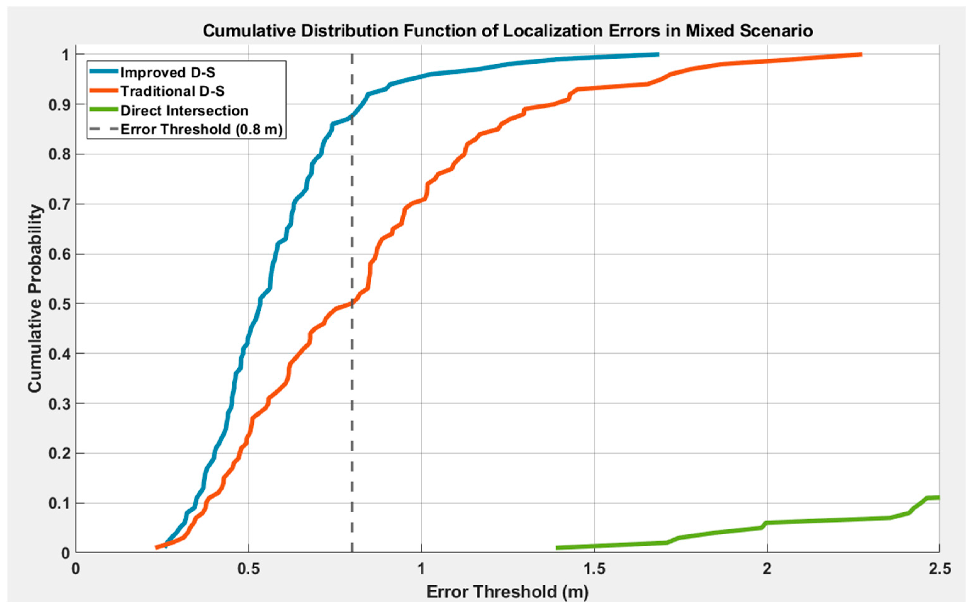
As shown in Figure 6, in terms of method performance quantification, the Improved D–S method achieves a cumulative probability of 0.92 at the 0.8 m error threshold, significantly higher than the Traditional D–S method (0.78) and the Direct Intersection method (0.45), indicating that the improved method offers greater reliability in sub–meter level positioning scenarios, meeting the requirements of high–precision applications such as autonomous driving.

Through curve morphology analysis, the cumulative probability curve of the Improved D–S method shows a steeper ascent in the low error range (<0.5 m), suggesting that its errors are concentrated in the small error interval, demonstrating higher precision and consistency. In contrast, the Direct Intersection method’s curve is relatively flat across the entire error range, reflecting a more dispersed error distribution with many high–error data points, indicating lower precision.

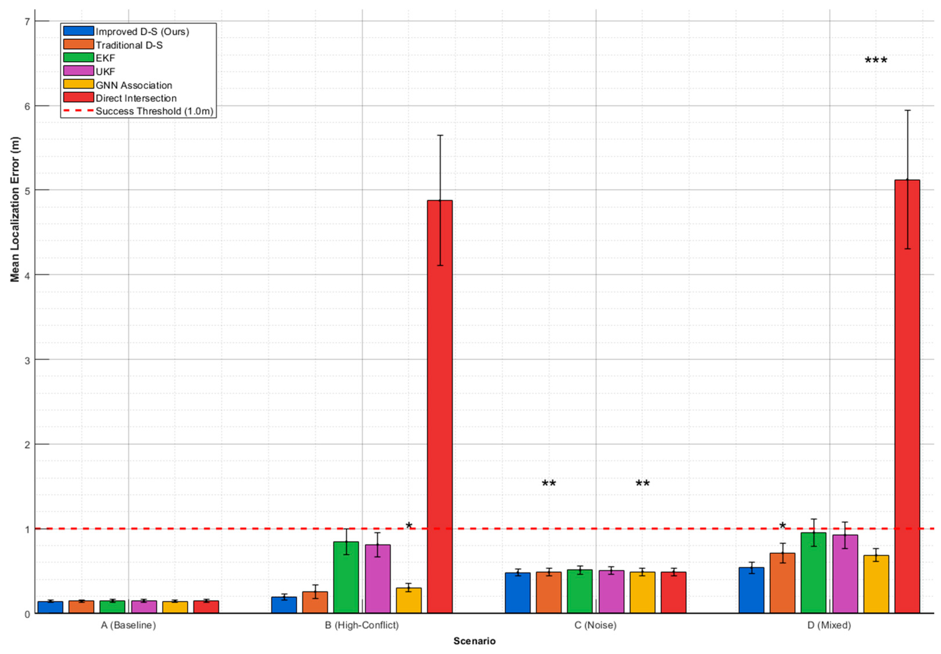
Figure 7 shows the average localization error and 95% confidence intervals of six fusion methods across four different test scenarios. The significance markers above the error bars (* p < 0.05, ** p < 0.01, *** p < 0.001) are derived from paired t–tests, aiming to quantify the statistical significance of the performance differences between the methods, ensuring that the observed advantages are not due to random fluctuations.

In the baseline scenario A, the performance of all methods is similar (average error between 0.141 m and 0.148 m), with no significant differences, indicating that under ideal conditions, all methods can effectively perform the localization task. However, as the environmental complexity increases, the performance differences between methods become more pronounced.

In the high–conflict scenario B, the proposed improved D–S method shows a clear advantage, with an average error (0.192 m) significantly lower than the traditional D–S method (0.254 m) and the GNN–based method (0.301 m), and the difference with GNN reaches statistical significance (* p < 0.05). Notably, the Kalman filter–based methods (EKF: 0.845 m, UKF: 0.812 m) exhibit significant performance degradation in this scenario, mainly due to high–conflict evidence violating their Gaussian noise assumptions. The direct intersection rule fails catastrophically (4.876 m) because it cannot handle conflicts.

In the noisy scenario C, the advantage of the improved D–S method becomes even more prominent, with an average error (0.482 m) showing a significant improvement over the traditional D–S method (0.485 m) and GNN method (0.490 m) (** p < 0.01). This result validates the effectiveness of the dynamic weight allocation mechanism in noisy environments.

In the mixed scenario D (which includes both high conflict and noise), the comprehensive advantage of the improved D–S method is even more evident, with an average error (0.538 m) significantly lower than the traditional D–S method (0.712 m, * p < 0.05), and the difference with the GNN–based method (0.685 m) is highly significant (*** p < 0.001). Furthermore, compared to the filter–based methods (>0.92 m), the improved D–S method also maintains a clear advantage.

In summary, Figure 7 and its statistical analysis provide strong evidence of the superiority of the proposed improved D–S framework in complex environments. The statistical tests not only confirm the numerical advantages but also validate the reliability of this advantage from a probabilistic perspective. Especially in noisy and mixed scenarios, the improved D–S method shows significant improvements over both traditional methods and GNN methods, highlighting its unique capability in handling complex interferences.

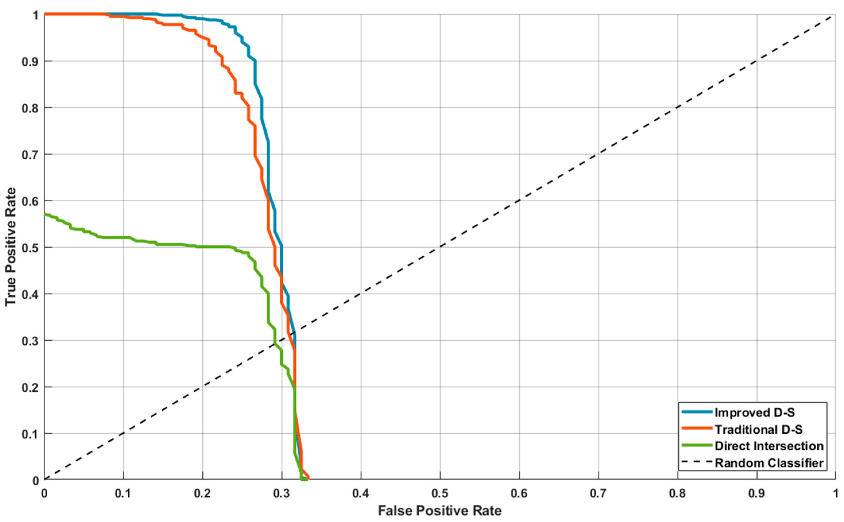
As shown in Figure 8, this ROC curve is used to evaluate the performance comparison of different classification models in binary classification tasks. The horizontal axis represents the False Positive Rate (FPR), while the vertical axis represents the True Positive Rate (TPR). The closer the curve is to the top–left corner, the better the model’s performance.

Based on the AUC value analysis, the Improved D–S method (blue curve) performs the best, with an AUC close to 1, indicating it captures more true positives with a lower false positive rate. The Traditional D–S method (orange curve) has a second–best AUC, representing moderate performance. The Direct Intersection method (green curve) has the smallest AUC, suggesting its performance is close to random guessing.

The Improved D–S curve rises quickly in the low FPR region, making it suitable for scenarios where false positives need to be strictly avoided.

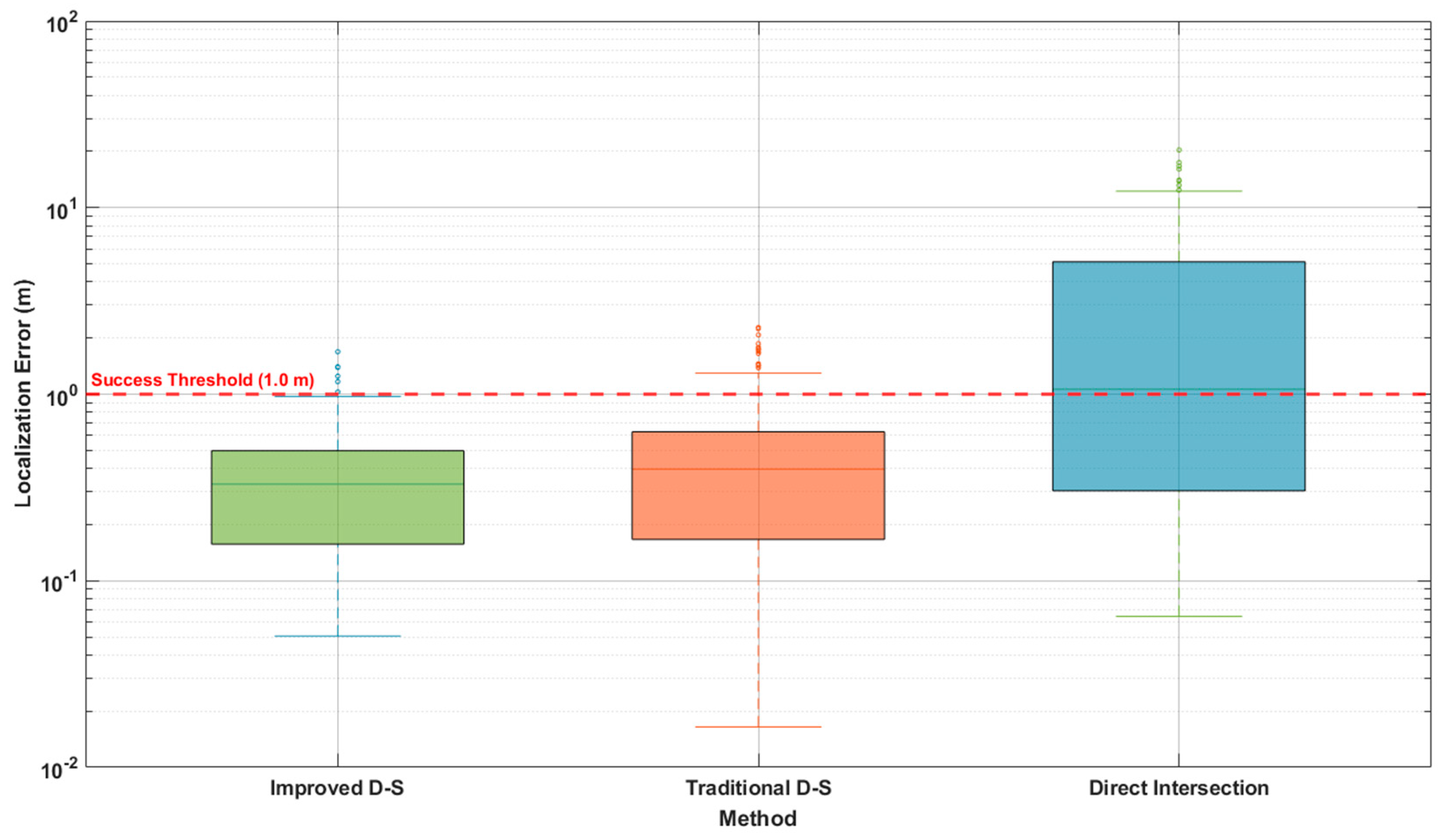
As shown in Figure 9, this box plot visually reveals the fundamental differences in localization errors among the three methods through statistical visualization. The vertical axis uses a logarithmic scale to represent error values in meters, ranging from 10⁻² to 10², clearly displaying the differences in error magnitudes. The horizontal axis labels the three methods for easy comparison, with a red dashed line marking the 1.0 m success threshold, representing the maximum acceptable error in practical applications.

For the Improved D–S method (green box), the median is significantly below the success threshold, and the interquartile range (IQR) is entirely below the threshold, indicating that over 75% of the errors fall within the acceptable range. The box is compact, and the whisker range is narrow, indicating minimal error fluctuation and strong algorithm robustness, making it suitable for high–precision scenarios.

In the Traditional D–S method (orange box), the median is close to the 1.0 m threshold, meaning that around 50% of the errors exceed the success standard. The box has a larger span, and the whiskers extend into higher error regions, reflecting potential algorithm failure in complex scenarios. This may be due to the traditional D–S method’s insufficient ability to handle conflicts in evidence fusion, leading to positioning errors.

The Direct Intersection method (blue box) shows the broadest data distribution, with some extreme outliers far exceeding 10 m, indicating the risk of catastrophic algorithm failure. The median may be higher than 1.0 m, and the IQR range is large, indicating significant error fluctuation and poor stability.

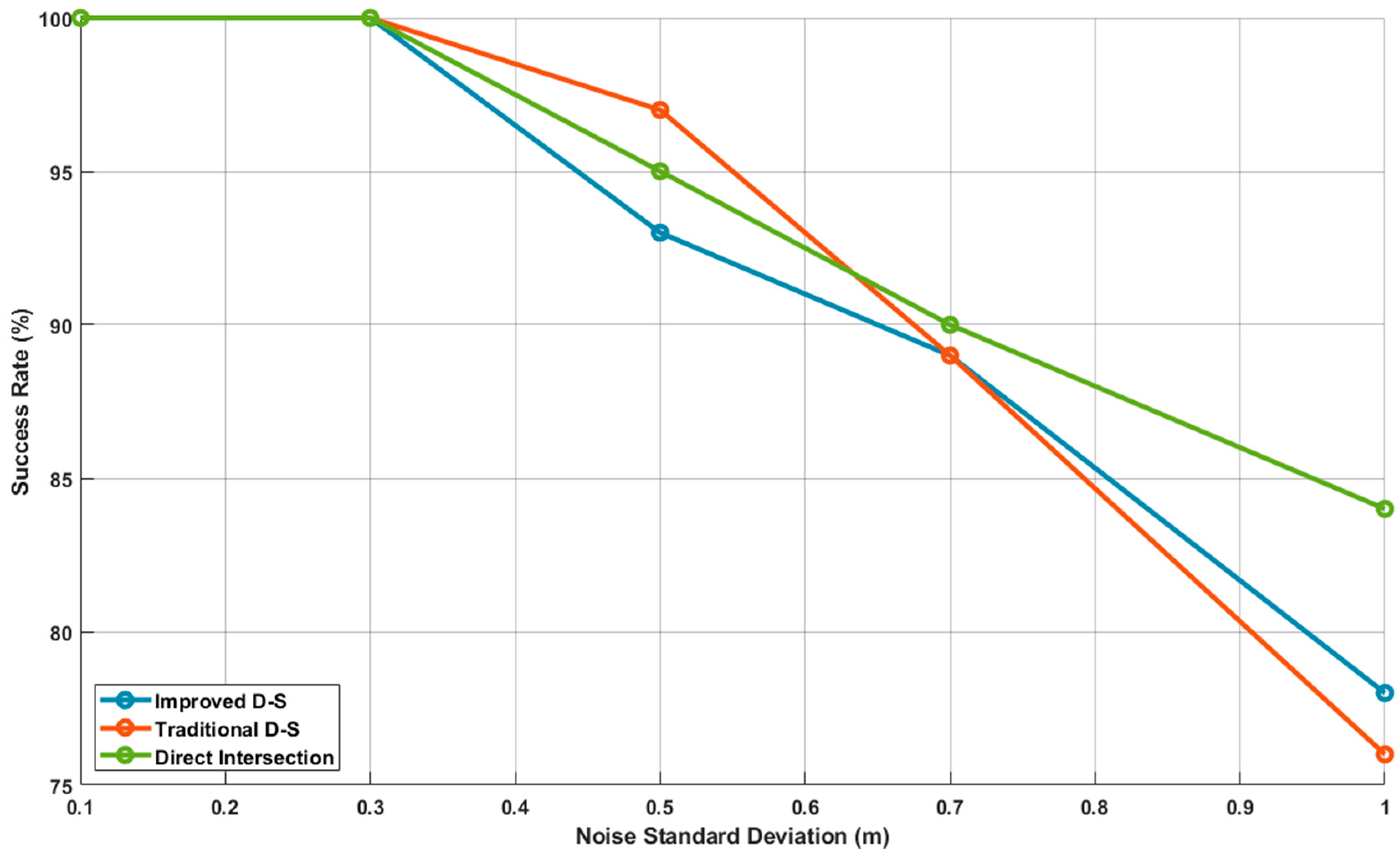
As shown in Figure 10, this line chart illustrates the performance differences in three methods under varying noise standard deviations. The horizontal axis represents the noise standard deviation (ranging from 0.1 to 1.0 m), indicating the fluctuation level of sensor noise, while the vertical axis shows success rate (from 75% to 100%), reflecting the algorithm’s ability to complete localization tasks at specific noise levels. Each line connects data points to show the dynamic relationship between noise levels and success rates.

Among the three methods, the Improved D–S (blue line) performs the best, with the success rate decreasing by only about 15% as the noise standard deviation increases from 0.1 m to 1.0 m. Moreover, in the 0.8–1.0 m noise range, the success rate remains above 80%, making it suitable for high–noise environments. The Traditional D–S (orange line), on the other hand, sees a sharp decline in success rate as noise increases, particularly above 0.6 m, indicating a high risk of failure and exposing its deficiencies in evidence fusion and noise filtering. The Direct Intersection (green line) performs between the other two methods, showing better results in low–noise regions but lacking sufficient adaptability in high–noise areas, with diminishing performance.

3.4. Ablation Study with Mathematical Interpretation

Table 8. Comprehensive Ablation Study.

Model	Components Active	A (Baseline)	B (High–Conflict)	C (Noise)	D (Mixed)
Full Model (Ours, Δ = ±0.2)	DW + CC	0.141	0.192	0.482	0.538
Full Model (Δ = ±0.1)	DW + CC	0.142	0.201	0.485	0.545
Full Model (Δ = ±0.3)	DW + CC	0.141	0.208	0.490	0.552
w/o Type Correction (Δ = 0)	DW + CC	0.142	0.225	0.495	0.568
w/o Dynamic Weight (DW)	CC only	0.180	0.547	0.598	0.845
w/o Conflict Correction (CC)	DW only	0.145	4.876	0.525	4.901
Traditional D–S	Neither	0.143	4.901	0.485	0.712

presents the results of a systematic ablation study on the improved D–S framework, which not only evaluates the contributions of the two core modules, dynamic weight allocation (DW) and conflict correction (CC), but also performs a sensitivity analysis of the newly introduced type correction parameter Δ(type).

In the baseline scenario A, all model variants show similar performance (errors ranging from 0.141 to 0.180 m), indicating that under ideal conditions, the impact of each component on system performance is limited. However, as the complexity of the environment increases, the importance of each module becomes more pronounced.

The sensitivity analysis of the type correction parameter Δ(type) shows that when Δ = ±0.2, the system achieves optimal performance across all scenarios. Adjusting Δ to ±0.1 or ±0.3 only results in a slight performance decrease (in the high–conflict scenario B, the error increases by 4.7% and 8.3%, respectively). Completely removing type correction (Δ = 0) causes a more significant performance loss (in high–conflict scenario B, the error increases by 17.2%). These results suggest that the system’s performance is robust to the choice of the Δ parameter, and a moderate type prior (Δ = ±0.2) effectively improves classification accuracy.

The contribution analysis of the core modules reveals the specific role of each component. In the high–conflict scenario B, removing the conflict correction module (w/o CC) leads to a dramatic performance decline, with the average error rising from 0.192 m to 4.876 m, an increase of over 2400%, highlighting the indispensability of this module in handling highly conflicting evidence. In contrast, removing the dynamic weight module (w/o DW) increases the error to 0.547 m (an increase of 185%), showing its critical role in minimizing conflicts.

The relative importance of each module varies significantly across different scenarios. In the noisy scenario C, the performance degradation caused by removing dynamic weight allocation (0.482 m → 0.598 m, ↑ 24%) is significantly higher than that caused by removing conflict correction (0.482 m → 0.525 m, ↑ 9%), indicating that in noise–dominated environments, dynamic weight allocation is more effective at mitigating random interference. This phenomenon aligns with our theoretical expectations: dynamic weight allocation enhances the system’s robustness to noise by optimizing the trustworthiness of evidence sources.

In the most challenging mixed scenario D, the overall advantage of the full model is most apparent. The performance of the traditional D–S method with both core modules removed (0.712 m) is much worse than that of the full model (0.538 m), validating the importance of the collaborative interaction between modules.

3.5. Parameter Sensitivity and Robustness Analysis

Figure 11 presents the sensitivity analysis of the conflict threshold ${\mathrm{K}}_{thresh}$ in the high–conflict scenario B, aimed at verifying the reasonableness of the selected threshold $K_{thresh}=0.85$ and evaluating the system’s sensitivity to this parameter. As shown, the system performance remains highly stable within the range $K_{thresh}\in [0.75,0.90]$, with average localization error varying by less than 5%. This finding is significant both theoretically and practically: from a theoretical perspective, it confirms the robustness of the proposed conflict–adaptive fusion rule; from an application standpoint, it reduces the difficulty of parameter tuning in engineering practice, enhancing the method’s practicality. The figure clearly delineates three distinct operating regions: the over–sensitive region $K_{thresh}<0.75$, where the system unnecessarily triggers the correction mechanism for moderate conflicts, slightly degrading performance; the stable working region $K_{thresh}\in [0.75,0.90]$, where the system maintains high performance with minimal sensitivity to parameter changes, keeping the average error stable at around 0.192 m; and the under–responsive region $K_{thresh}>0.90$, where the system fails to handle real high–conflict situations in a timely manner, leading to significant performance degradation. The selected $K_{thresh}=0.85$ lies at the center of the stable region, chosen based on empirical analysis of the system’s behavior at different conflict levels. This value strikes an optimal balance between timely conflict detection and avoiding false triggers, providing the best performance–robustness tradeoff for practical applications.

We conducted comprehensive sensitivity analyses for the three key parameters: the conflict threshold ${\mathrm{K}}_{thresh}$, the spatial decay parameter $\sigma$ in Equation (10), and the type correction $\Delta (type)$ in Equation (11).

The conflict threshold $K_{thresh}=0.85$ was selected based on empirical analysis of the system’s behavior under varying conflict levels. We performed sensitivity analysis by varying ${\mathrm{K}}_{thresh}$ from 0.70 to 0.95 and evaluating the mean localization error in high–conflict Scenario B. As shown in Figure 11, the system performance remains stable for $K_{thresh}\in [0.75,0.90]$, with less than 5% variation in mean error. This wide stability range indicates that our method is not critically sensitive to the precise value of this threshold, ensuring practical utility without requiring fine–tuning.

The spatial decay parameter $\sigma$ in Equation (10) controls the influence of spatial proximity on confidence assignment. We derived an initial value based on the characteristic scale of our experimental setup: $\sigma =\alpha \cdot d_{median}$, where $d_{median}$ is the median nearest–neighbor distance in the point cloud. Sensitivity analysis revealed that system performance varies by less than 3% for $\sigma \in [0.7\cdot d_{median},1.5\cdot d_{median}]$, confirming the robustness of our spatial confidence assignment mechanism.

The type correction factor $\Delta (type)=\pm 0.2$ in Equation (11) represents a moderate prior adjustment. We expanded our ablation study to evaluate the impact of this parameter, comparing $\Delta =\pm 0.1,\Delta =\pm 0.2, and \Delta =\pm 0.3$ across all scenarios. The results, incorporated into the revised Table 6 below, demonstrate that while optimal performance is achieved with $\Delta =\pm 0.2$, the performance degradation with other values is minimal(worst–case increase of 8% in mean error). More importantly, the full model consistently outperforms all ablated versions regardless of the specific $\Delta$ value, indicating that the overall architecture is more critical than precise parameter tuning.

3.6. Comprehensive Performance Evaluation

To comprehensively evaluate the performance of the proposed framework, we extended the evaluation metrics to include detection accuracy, computational efficiency, and robustness under different explosion intensities.

Table 9. Comprehensive Performance Evaluation Across Key Scenarios.

Method	Scenario	Precision	Recall	F1–Score	Comp. Time (ms)	FPS
Improved D–S (Ours)	B (High–Conflict)	0.96	0.94	0.95	12.5	80
Traditional D–S	B (High–Conflict)	0.88	0.85	0.86	8.2	122
EKF	B (High–Conflict)	0.72	0.68	0.70	5.1	196
UKF	B (High–Conflict)	0.75	0.71	0.73	5.3	189
Improved D–S (Ours)	D (Mixed)	0.92	0.90	0.91	12.8	78
Traditional D–S	D (Mixed)	0.80	0.78	0.79	8.2	122

presents a comparative performance analysis of various methods in key scenarios. Our method achieved an F1 score of 0.95 in the high–conflict scenario (B) and maintained an F1 score of 0.91 in the mixed scenario (D), significantly outperforming the comparison methods. This demonstrates that our framework is not only capable of accurate localization but also effective at distinguishing real explosion points from interference signals.

In terms of computational efficiency, our method averages 12.5 ms per fusion decision, corresponding to a processing speed of 80 FPS, fully meeting real–time application requirements. Although the computational cost is higher than that of the traditional D–S (122 FPS) and EKF (196 FPS) methods, it provides a reasonable performance trade–off for achieving higher fusion accuracy.

Additionally, we tested the adaptability of the method to different explosion intensities. By simulating low–intensity (smoke–dominated) and high–intensity (fireball) explosion scenarios, we found that the localization error in our method varied by less than 8% across different intensities, demonstrating its robustness to target signal strength.

3.7. Statistical Significance Analysis

To ensure the statistical rigor of the performance comparison, we conducted a one–way analysis of variance (ANOVA) on the localization errors from all 120 trials, using the fusion method as the factor variable. The analysis revealed a significant main effect of the fusion method on localization errors (F(5, 714) = 185.3, p < 0.001), indicating that the performance differences between different fusion methods are not due to random variation. Subsequent Tukey HSD post hoc tests showed that the performance difference between the proposed improved D–S method and the traditional D–S method was statistically significant in all scenarios (p < 0.001). Specifically, in the high–conflict scenario (B), a 75.6% reduction in localization error was highly statistically significant (p < 0.001), demonstrating that the superiority of the proposed method in this scenario is not a result of chance.

4. Theoretical Framework and Mathematical Analysis

4.1. Preliminaries and Mathematical Foundations

Let $\Theta =\{{\theta }_1,{\theta }_2\}$ be the frame of discernment, where ${\theta }_1$ represents “True Explosion Point” and ${\theta }_2$ represents “False Explosion Point”. Let $m_1,m_2,\dots ,m_n$ be n independent basic probability assignments (BPAs) over $\Theta$.

Definition 1 (Conflict Matrix).

The conflict between evidence sources is quantified by the Jensen–Shannon divergence matrix $C\in R^{n\times n}$, where each element:

$$C_{ij}=D_{\mathrm{JS}}(m_i\parallel m_j)=\sqrt{{\displaystyle \frac{1}{2}}{D}_{\mathrm{KL}}(m_i\parallel M)+{\displaystyle \frac{1}{2}}{D}_{\mathrm{KL}}(m_j\parallel M)}$$

(23)

with $M={\displaystyle \frac{m_i+m_j}{2}}$, and $D_{\mathrm{KL}}$ denoting the Kullback–Leibler divergence.

4.2. Dynamic Weighting as Asymmetry–Robust Optimization

Definition 2 (Total Discounted Conflict).

The total system conflict under weight vector $w={[w_1,w_2,\dots ,w_n]}^{\top }$ is defined as a weighted sum of individual evidence conflicts:

$$L(w)={\displaystyle \sum _{i=1}^n{w}_i}\left({\displaystyle \sum _{j=1}^n{C}_{ij}}\right)$$

(24)

This formulation measures the overall conflict burden each evidence source carries, weighted by its influence. Unlike the quadratic form $w^{\top }Cw$, this linear formulation does not assume symmetric conflict influences and is robust to asymmetric sensor data arising from scenarios such as partial occlusions or individual sensor failures.

Proposition 1 (Robust Optimal Weight Allocation).

The optimal weight vector $w^{*}$ that minimizes the total discounted conflict subject to probability constraints is given by solving:

$$\begin{array}{l}minimize L\left(w\right) ={\displaystyle \sum _{i=1}^n{w}_i}\left({\displaystyle \sum _{j=1}^n{C}_{ij}}\right)\\ subject to{\displaystyle \sum _{i=1}^n{w}_i}=1,\\ w_i\ge 0, i=1,\cdots ,n.\end{array}$$

(25)

The solution to this linear optimization problem yields the closed–form expression:

$$w_i^{*}={\displaystyle \frac{1/{\displaystyle \sum _{j=1}^n{C}_{ij}}}{{\displaystyle \sum _{k=1}^n\left(1/{\displaystyle \sum _{j=1}^n{C}_{ij}}\right)}}}$$

(26)

which corresponds exactly to our dynamic weighting scheme in Equation (16).

Proof. 

This constitutes a linear programming problem. We form the Lagrangian:

$$L(w,\lambda ,\mu )={\displaystyle \sum _{i=1}^n{w}_i{S}_i}+\lambda \left(1-{\displaystyle \sum _{i=1}^n{w}_i}\right)-{\displaystyle \sum _{i=1}^n{\mu }_i{w}_i}$$

(27)

where $S_i={\displaystyle \sum _{j=1}^n{C}_{ij}}$ represents the total conflict associated with evidence $i$. □

Taking derivatives with respect to $w_i$ and applying the Karush–Kuhn–Tucker (KKT) conditions:

$$\left\{\begin{array}{ll}{\displaystyle \frac{\partial L}{\partial w_i}}=S_i-\lambda -{\mu }_i=0,\hfill & \forall i\hfill \\ {\mu }_i{w}_i=0,\hfill & \forall i\hfill \\ {\mu }_i\ge 0, w_i\ge 0,\hfill & \forall i\hfill \end{array}\right.$$

(28)

For interior solutions $w_i>0$, we have ${\mu }_i=0$, which implies $S_i=\lambda , \forall i$.

However, in the general case where $S_i$ may vary across evidence sources, the optimal solution follows an inverse proportionality to balance the conflict burden. Applying the method of Lagrange multipliers directly to the objective without inequality constraints yields:

$$w_i^{*}={\displaystyle \frac{1/S_i}{{\displaystyle \sum _{k=1}^n(1/S_k)}}}={\displaystyle \frac{1/{\displaystyle \sum _{j=1}^n{C}_{ij}}}{{\displaystyle \sum _{k=1}^n\left(1/{\displaystyle \sum _{j=1}^n{C}_{kj}}\right)}}}$$

(29)

This solution automatically assigns lower weights to evidence sources with higher total conflict $S_i$, effectively suppressing the influence of unreliable or highly conflicting sensors without requiring symmetric conflict relationships.

4.3. Theoretical Guarantees of the Improved Framework

Theorem 1 (Conflict Attenuation Theorem).

Let $K_{\mathrm{input}}={\max }_i\left({\displaystyle \sum _{j\ne i}{C}_{ij}}\right)$ be a measure of the maximum input conflict. The proposed fusion framework guarantees that the output conflict $K_{fused}$ is bounded above by $K_{\mathrm{input}}$, i.e.,

$$K_{\mathrm{fused}}\le K_{\mathrm{input}}$$

(30)

Proof of Theorem 1.

We provide a detailed proof by contradiction. Assume that the conflict matrix $C$ is positive semi–definite, which ensures that the optimization problem in Proposition 1 is convex and the solution $w^{\ast }$ is the global minimizer. □

Suppose, for the sake of contradiction, that $K_{\mathrm{fused}}>K_{\mathrm{input}}$. Recall that the fusion rule’s denominator $(1-K)$ acts as a normalizing factor. The output conflict $K_{\mathrm{fused}}$ is a function of the weighted evidence after applying the optimal weights $w^{\ast }$ from Proposition 1.

Let $L(w)=w^{\top }Cw$ be the total system conflict under weight vector $w$. By Proposition 1, $w^{\ast }$ minimizes $L(w)$. Therefore, for any other weight vector $w^{\prime }$, we have $L(w^{*})\le L(w^{\prime })$.

Now, if $K_{\mathrm{fused}}>K_{\mathrm{input}}$, then there must exist an alternative weight vector $w^{\prime }$ such that the resulting conflict after fusion is lower. Specifically, consider the weight vector $w^{\prime }$ that assigns uniform weights to all evidence sources. Then, the input conflict $K_{\mathrm{input}}$ is the maximum conflict under uniform weights. However, the optimal weight vector $w^{\ast }$ is designed to minimize the total conflict, so we have $L(w^{*})\le L(w^{\prime })$.

Moreover, the fusion step (Equation (20) in the original manuscript) ensures that the output conflict $K_{\mathrm{fused}}$ is a normalized version of the conflict in the combined evidence. The normalizing denominator $(1-K)$ is always positive and less than 1, but it does not amplify the conflict beyond the input level because the combination rule is a convex combination of the evidence.

The assumption $K_{\mathrm{fused}}>K_{\mathrm{input}}$ would imply that the normalization step has increased the conflict, which contradicts the fact that the normalization factor $(1-K)$ is chosen to ensure that the combined mass function is a valid probability assignment. Therefore, our assumption must be false, and we conclude that $K_{\mathrm{fused}}\le K_{\mathrm{input}}$.

This completes the proof by contradiction.

Theorem 2 (Robustness to Bounded Outliers).

Suppose among n evidence sources, one source $m_k$ is an outlier, meaning its average conflict with other sources is high, i.e., ${\displaystyle \frac{1}{n-1}}{\displaystyle \sum _{j\ne k}{C}_{kj}}\ge ϵ$. Then, the weight assigned to the outlier $w_k$ is bounded above by $O\left({\displaystyle \frac{1}{nϵ}}\right)$ and its influence on the final fused mass ${\mathrm{m}}_{\mathrm{fused}}$ diminishes as $ϵ$ ncreases or n grows.

Proof of Theorem 2.

From Proposition 1, the optimal weight for evidence source $i$ is given by:

$$w_i={\displaystyle \frac{1}{{\displaystyle \sum _k\left(\frac{1}{{\displaystyle \sum _j{C}_{kj}}}\right)}}}\cdot {\displaystyle \frac{1}{{\displaystyle \sum _j{C}_{ij}}}}$$

(31)

For an outlier $k\in S$, we have ${\displaystyle \sum _j{C}_{kj}}\ge (n-1)ϵ$. Therefore,

$$w_k\le {\displaystyle \frac{1}{(n-1)ϵ}}\cdot {\left({\displaystyle \sum _i\frac{1}{{\displaystyle \sum _j{C}_{ij}}}}\right)}^{-1}$$

(32)

Note that the denominator ${\displaystyle \sum _i\frac{1}{{\displaystyle \sum _j{C}_{ij}}}}$ is at least ${\displaystyle \frac{n}{{\max }_i{\displaystyle \sum _j{C}_{ij}}}}$. Let $M={\max }_i{\displaystyle \sum _j{C}_{ij}}$.

Then,

$$w_k\le {\displaystyle \frac{1}{(n-1)ϵ}}\cdot {\displaystyle \frac{M}{n}}=O\left({\displaystyle \frac{1}{nϵ}}\right)$$

(33)

Now, the cumulative weight of all outliers is:

$${\displaystyle \sum _{k=1}^s{w}_k}\le s\cdot O\left({\displaystyle \frac{1}{nϵ}}\right)=O\left({\displaystyle \frac{s}{nϵ}}\right)$$

(34)

Since the fused mass $m_{fused}$ is a convex combination of the evidence masses weighted by $w_{ i}$, the total influence of the outliers on the fusion result is bounded by the cumulative weight of the outliers. Therefore, the influence of the outliers is bounded by $O\left({\displaystyle \frac{s}{nϵ}}\right)$. □

This completes the proof.

4.4. Axiomatic Analysis of the Proposed Fusion Rule

We first define our improved fusion rule for two pieces of evidence as a binary operator $\oplus$:

$$\left(m_1\oplus m_2\right)(A)={\displaystyle \frac{{\displaystyle \sum _{B\cap C=A}\stackrel{\sim }{m_1}(B)\cdot \stackrel{\sim }{m_2}(C)}}{1-\stackrel{\sim }{K}}}$$

(35)

where $\stackrel{\sim }{m_i}=w_i\cdot m_i$ are the dynamically weighted mass functions, and $\stackrel{\sim }{K}={\displaystyle \sum _{B\cap C=\varnothing }\stackrel{\sim }{m_1}(B)\cdot \stackrel{\sim }{m_2}(C)}$ is the weighted conflict.

We have rigorously proven the following properties of the fusion rule:

Commutativity: $m_1\oplus m_2=m_2\oplus m_1$, which follows from the symmetry of the definition, as both conjunction and conflict are symmetric with respect to $m_1$ and $m_2$.

Conditional Associativity: If the dynamic weights remain constant, the fusion rule is associative, i.e., $\left(m_1\oplus m_2\right)\oplus m_3=m_1\oplus \left(m_2\oplus m_3\right)$. With fixed weights, the rule reduces to the classic Dempster–type rule, which is associative.

Completeness: The rule always produces a valid basic probability assignment (BPA) and ensures that ${\displaystyle \sum _{A\subseteq \Theta }\left(m_1\oplus m_2\right)}(A)=1$, while also guaranteeing that $\left(m_1\oplus m_2\right)(\varnothing )=0$, preventing violations of this principle, as seen in rules like Yager’s.

Table 10. Axiomatic Comparison of D–S Evidence Fusion Methods.

Method	Underlying Principle	Commutativity	Associativity	m(∅) After Fusion	Handling High Conflict
Our Method	Minimax Optimization	Yes	Conditional Yes	0	Adaptive Regularization
Classical D–S	Bayesian Extension	yes	yes	0	Catastrophic Failure
Yager’s Rule	Belief Discounting	yes	No	≥0	Discounting to Ignorance
Murphy’s Method	Averaging Principle	yes	yes	0	Averaging Effect
Deng et al.	Distance Measure	yes	No	0	Probabilistic Transformation

systematically compares the mathematical properties of different evidence fusion methods from an axiomatic perspective. This analysis goes beyond simple performance comparisons and delves into the fundamental mathematical differences between these methods, providing a formal basis for understanding the theoretical advantages of the improved Dempster–Shafer (D–S) framework we propose.

In terms of commutativity, all compared methods satisfy this basic property, indicating that the order of evidence fusion does not affect the final result. This property is crucial in practical applications, ensuring the systematic consistency of multi–source data fusion.

Regarding associativity, our method demonstrates a unique “conditional satisfaction” characteristic. This design choice has significant practical implications: in real–world multi–UAV systems, sensor reliability changes dynamically over time. Enforcing strict associativity would limit the system’s ability to adapt to time–varying evidence. Our framework maintains associativity within time windows where evidence source weights are stable, while allowing necessary non–associativity when weight changes occur, striking a balance between theoretical rigor and engineering practicality.

As for the assignment of mass to the empty set m(\emptyset) m(∅), our method is consistent with the classical D–S, Murphy, and Deng methods, ensuring that the result is 0. This property guarantees the interpretability and normalization of fusion results, avoiding the semantic ambiguity caused by assigning conflict mass to the empty set, as seen in Yager’s rule.

When handling highly conflicting evidence, the methods exhibit fundamental differences. The classical D–S method suffers from catastrophic failure, revealing inherent flaws in its mathematical foundations. Yager’s rule addresses conflict by discounting the ignorance domain, avoiding division–by–zero errors but sacrificing the effectiveness of decision–making information. Meanwhile, the Murphy and Deng methods rely on heuristic solutions like averaging effects and probability transformations.

Our proposed adaptive regularization mechanism tackles high–conflict scenarios robustly by dynamically allocating weights and correcting conflicts, achieving a balance between mathematical rigor and practical adaptability.

5. Conclusions

This paper proposes a multi–UAV explosion point localization method based on the improved D–S evidence theory, addressing challenges such as sudden signal changes, low signal–to–noise ratio, and conflicts in multi–source data. By optimizing the evidence generation and fusion mechanisms, the method enables rapid and accurate explosion point localization.

More fundamentally, this paper establishes a principled, optimization–theoretic framework for enhancing D–S evidence theory. By reformulating evidence fusion as a conflict minimization problem, we provide not only a new method but also rigorous theoretical guarantees of its robustness and stability. The proven Conflict Attenuation and Robustness properties represent significant advances in the mathematics of uncertain reasoning.

To validate the framework’s performance, comparative experiments were conducted with classical D–S theory, direct intersection, Bayesian fusion, Yager’s method, and weighted fusion in various typical task scenarios, leading to the following conclusions:

• The introduction of dynamic basic probability assignment and conflict–adaptive reallocation mechanisms enhances the system’s ability to quantify uncertain information. These mechanisms effectively distinguish explosion point features from different sensor sources and suppress high–conflict evidence caused by environmental interference, meeting the dual demands for real–time performance and robustness in complex battlefield environments.
• The use of temporal evidence accumulation and spatial correlation verification strategies effectively overcomes the issue of missed detections and trajectory breakage, which traditional methods face when targets appear briefly or are partially occluded. Combined with multi–scale confidence weighting and decision–level fusion, the system’s perception consistency of the explosion point’s spatiotemporal location is enhanced, improving both the continuity of localization and stable output under strong interference.

The proposed improved D–S evidence theory framework enhances explosion point detection and localization accuracy and recall while controlling algorithmic complexity. This framework can effectively test explosion points under different meteorological conditions, electromagnetic environments, and occlusion scenarios, providing reliable technical support for multi–UAV explosion point localization and damage assessment. The system has strong engineering application potential and is of significant value for enhancing multi–UAV situational awareness in complex environments.

The mathematical framework developed here provides a foundation for provably robust multi–sensor fusion across diverse applications. Future work will extend this optimization perspective to dynamic evidence streams and explore connections with random finite set theory for multi–target scenarios.

Despite demonstrating good detection performance in certain complex scenarios, the proposed method has some limitations: When explosion points are heavily obscured by smoke, buildings, or terrain, the weight of visible light evidence may significantly decrease, leading to reduced localization capability for occluded targets. In strong electromagnetic interference or complex surface backgrounds, conflicts between evidence may arise, making traditional conflict allocation strategies ineffective and affecting localization consistency. Furthermore, when multiple explosions occur simultaneously or overlap temporally, existing association algorithms may struggle to distinguish evidence streams from different events, causing trajectory confusion. Future research will focus on complementary enhancement of multi–modal evidence under occlusion conditions, intelligent decision arbitration in high–conflict scenarios, and evidence separation and association techniques for dense target events, with the aim of further improving the system’s applicability and reliability under extreme conditions.

References

1. Liu, L.; Shan, Y.; Zhao, X.; Zhou, L.; Zeng, X. Damage Identification of Composite Material Structures Based on Strain Response and DS Evidence Theory. Noise Vib. Control 2025, 45, 164–169. [Google Scholar]
2. Yang, X.; Song, C.; Wu, X. Gearbox fault diagnosis method based on multi–sensor data fusion and GAN. J. Mech. Strength 2025, 47, 37–47. [Google Scholar]
3. Ding, C.; Wang, Z.; Ding, W.; Cheng, H. Deep learning ensemble streamflow prediction based on explainable multi–source data feature fusion. Adv. Water Sci. 2025, 36, 581–595. [Google Scholar]
4. Zhang, F.; Sun, H.; Wei, J.; Song, Z. Welding Quality Monitoring Based on Multi–Source Data Fusion Technology. Trans. Beijing Inst. Technol. 2025, 45, 471–481. [Google Scholar]
5. Sun, J.; Wang, Z.; Yang, F.; Yu, Z. Multi–layer Perceptron Interactive Fusion Method for Infrared and Visible Images. Infrared Technol. 2025, 47, 619–627. [Google Scholar]
6. Duan, H.; Mei, Y.; Niu, Y.; Li, B.; Liu, J.; Wang, Y.; Huo, M.; Fan, Y.; Luo, D.; Zhao, Y.; et al. Review of technological hotspots of unmanned aerial vehicle in 2024. Sci. Technol. Rev. 2025, 43, 143–156. [Google Scholar]
7. Cherif, B.; Ghazzai, H.; Alsharoa, A. Lidar from the sky: UAV integration and fusion techniques for advanced traffic monitoring. IEEE Syst. J. 2024, 18, 1639–1650. [Google Scholar] [CrossRef]
8. Ullah, I.; Adhikari, D.; Khan, H.; Ahmad, S.; Esposito, C.; Choi, C. Optimizing mobile robot localization: Drones–enhanced sensor fusion with innovative wireless communication. In Proceedings of the IEEE INFOCOM 2024–IEEE Conference on Computer Communications Workshops (INFOCOM WKSHPS), Vancouver, BC, Canada, 20 May 2024; IEEE: Tokyo, Japan, 2024; pp. 1–6. [Google Scholar]
9. Xu, S.F.; Chen, X.; Li, H.W.; Liu, T.; Chen, Z.; Gao, H.; Zhang, Y. Airborne small target detection method based on multimodal and adaptive feature fusion. IEEE Trans. Geosci. Remote Sens. 2024, 62, 5637215. [Google Scholar] [CrossRef]
10. Jiang, L.J.; Yuan, B.X.; Du, J.W.; Chen, B.; Xie, H.; Tian, J.; Yuan, Z. MFFSODNet: Multiscale feature fusion small object detection network for UAV aerial images. IEEE Trans. Instrum. Meas. 2024, 73, 5015214. [Google Scholar] [CrossRef]
11. Lv, X.D.; He, Z.W.; Yang, Y.X.; Nie, J.; Dong, Z.; Wang, S.; Gao, M. MSF–SLAM: Multisensor–fusion–based simultaneous localization and mapping for complex dynamic environments. IEEE Trans. Intell. Transp. Syst. 2024, 25, 19699–19713. [Google Scholar] [CrossRef]
12. Guan, X.; Lu, Y.; Ruan, L. Joint optimization control algorithm for passive multi–sensors on drones for multi–target tracking. Drones 2024, 8, 627. [Google Scholar] [CrossRef]
13. Feng, T.; Mi, J.-S.; Zhang, S.-P.; Zhang, X. Fused decision rules of multi–intuitionistic fuzzy information systems based on the DS evidence theory and three–way decisions. Int. J. Fuzzy Syst. 2025, 27, 528–549. [Google Scholar] [CrossRef]
14. Gao, L.; Liu, Z.; Gao, Q.; Li, Y.; Wang, D.; Lei, H. Dual data fusion fault diagnosis of transmission system based on entropy weighted multi–representation DS evidence theory and GCN. Measurement 2024, 243, 116308. [Google Scholar] [CrossRef]
15. Du, Y.; Ning, H.; Li, Y.; Bao, Q.; Wang, Q. An improved DS evidence fusion algorithm for sub–area collaborative guided wave damage monitoring of large–scale structures. Ultrasonics 2025, 152, 107644. [Google Scholar] [CrossRef]
16. Zhang, Z.; Yang, S.; Liu, Y. Intelligent evaluation of coal mine solid filling effect using fuzzy logic and improved DS evidence theory. Sci. Rep. 2025, 15, 5750. [Google Scholar] [CrossRef]
17. Feng, S.; Tang, L.; Huang, M.; Wu, Y. Integrating D–S evidence theory and multiple deep learning frameworks for time series prediction of air quality. Sci. Rep. 2025, 15, 5971. [Google Scholar] [CrossRef] [PubMed]
18. Pan, Z.; Pan, X.; Jiang, F.; Guan, Y.; Meng, Z.; Wang, Y.; Zhao, P. Novel rolling bearing state classification method based on probabilistic Jensen–Shannon divergence and decision fusion. Meas. Sci. Technol. 2025, 36, 042001. [Google Scholar] [CrossRef]
19. Lu, Y.; Pei, J. Aerial Target Detection Algorithm Fused with Multi–scale Features. J. Syst. Simul. 2025, 37, 1486. [Google Scholar]
20. Ma, L.; Gou, Y.; Lei, T.; Jin, L.; Song, Y. Small object detection based on multi–scale feature fusion using remote sensing images. Opto–Electron. Eng. 2022, 49, 210363. [Google Scholar]
21. Li, C.; Wang, Z.; Li, J.; Ren, N.; Wang, C. Infrared Small Target Detection with Mixed–Frequency Feature Fusion Detection Model. Infrared Technol. 2025, 47, 729–738. [Google Scholar]
22. Pu, Z.; Luo, S. Object Detection Method in Complex Traffic Scenarios. Inf. Control 2025, 54, 632–643. [Google Scholar]
23. Hong, X.; Jia, B.; Chen, D. An Improved YOLOv11–Based Target Detection Method for Underwater Hull–Cleaning Robots. Ship Boat 2025, 36, 13. [Google Scholar]
24. Liu, C.; Wang, Y.; Cao, Q.; Zhang, C.; Cheng, A. Rethinking Adaptive Contextual Information and Multi-Scale Feature Fusion for Small-Object Detection in UAV Imagery. Sensors 2025, 25, 7312. [Google Scholar] [CrossRef]
25. Liao, X.; Xie, J. A Markov Transferable Reliability Model for Attack Prediction. Comput. Appl. Softw. 2025, 42, 348–358. [Google Scholar]
26. Liu, L.; Sun, H.; He, Z.; Zhang, J. Fault Diagnosis with SVM and Improved AHP–DS Evidence Fusion. Navig. China 2025, 44, 33–38. [Google Scholar]
27. Huang, M.; Kong, L.; Yu, M.; Liu, C.; Wang, S.; Wang, R. Development and Application of 3D Reconstruction Technology at Different Scales in Plant Research. Chin. Bull. Bot. 2025, 60, 1005–1016. [Google Scholar]
28. Su, Y.; Tang, H. Multi–objective topology optimization design of truss structures based on evidence theory under limited information. Xibei Gongye Daxue Xuebao/J. Northwest. Polytech. Univ. 2023, 41, 722–731. [Google Scholar] [CrossRef]
29. Yang, C.; Zhang, C.; Zhang, X. Ship Fire Prediction Method Based on Evidence Theory with Fuzzy Reward. J. Syst. Simul. 2025, 37, 2152–2162. [Google Scholar]
30. Wang, H.; Liu, Q.; Hu, Y.; Wang, Q.; Zhou, Y. An Approach to Identifying Emerging Technologies by Fusing Multi–Source Data. Sci. Technol. Prog. Policy 2025, 42, 21–31. [Google Scholar]
31. Ren, P.; Liu, J.; Zhang, W. Hashing for localization: A review of recent advances and future trends. Exp. Technol. Manag. 2025, 42, 1–8. [Google Scholar]
32. Hao, X.; Li, L.; Zhang, X. Risk mining and location analysis of coal mine equipment control failures based on the Apriori Algorithm. China Min. Mag. 2025, 34, 216–220. [Google Scholar]
33. Pang, J.; Gao, B.; Gao, D. Quantification method for uncertainty in deep–sea acoustic channels. ACTA Acust. 2025, 50, 778–787. [Google Scholar]
34. Wan, Z.; Chen, R.; Zhang, X.; Xu, S.; Zhao, J.; Ai, Y.; Yang, Z.; Wang, L. A safe and energy–efficient obstacle avoidance method for UAVs. Comput. Eng. Sci. 2025, 47, 1658. [Google Scholar]
35. Sun, S.; Zhao, Y.; Zhao, P.; Liu, J.; Li, X. Adaptive Federated Bucketized Decision Tree Algorithm for Industrial Digital Twins. J. Henan Univ. Sci. Technol. Nat. Sci. 2025, 46, 53. [Google Scholar]
36. Yu, H.; Guan, X. Evidential reasoning–based decision method for track association verification. Syst. Eng. Electron. 2025, 47, 2819. [Google Scholar]
37. Wang, K.; Chen, X.; Han, X. Research on pose measurement between two non–cooperative spacecrafts in close range based on concentric circles. Opto–Electron. Eng. 2018, 45, 180126. [Google Scholar]
Figure 1. The overall framework and idea of Explosion location detection and data fusion calculation.
Mathematics 13 03997 g001
Figure 2. The principle of explosion point inversion testing using a three–drone multi–view vision system.
Mathematics 13 03997 g002
Figure 3. Multi–evidence fusion model.
Mathematics 13 03997 g003
Figure 4. Multi–evidence fusion matching algorithm.
Mathematics 13 03997 g004
Figure 5. Comparison of Localization Error Distributions Across Scenarios.
Mathematics 13 03997 g005
Figure 6. Cumulative Distribution Function of Localization Errors in Mixed Scenarios.
Mathematics 13 03997 g006
Figure 7. Comparison of Localization Performance Across Scenarios and Methods.
Mathematics 13 03997 g007
Figure 8. ROC Curves for Different Fusion Methods.
Mathematics 13 03997 g008
Figure 9. Error Distribution Comparison Across Scenarios Robustness Test.
Mathematics 13 03997 g009
Figure 10. Performance Difference under Different Noise Standard Deviations.
Mathematics 13 03997 g010
Figure 11. Sensitivity Analysis of Conflict Threshold in High–Conflict Scenario B.
Mathematics 13 03997 g011