Multiscale Bootstrap Correction for Random Forest Voting: A Statistical Inference Approach to Stock Index Trend Prediction

Abstract

This paper proposes a novel multiscale random forest model for stock index trend prediction, incorporating statistical inference principles to improve classification confidence. Traditional random forest classifiers rely on majority voting, which can yield biased estimates of class probabilities, especially under small sample sizes. To address this, we introduce a multiscale bootstrap correction mechanism into the ensemble framework, enabling the estimation of third-order accurate approximately unbiased p-values. This modification replaces naive voting with statistically grounded decision thresholds, improving the robustness of the model. Additionally, stepwise regression is employed for feature selection to enhance generalization. Experimental results on CSI 300 index data demonstrate that the proposed method consistently outperforms standard classifiers, including standard random forest, support vector machine, and weighted k-nearest neighbors model, across multiple performance metrics. The contribution of this work lies in the integration of hypothesis testing techniques into ensemble learning and the pioneering application of multiscale bootstrap inference to financial time series forecasting.

1. Introduction

The prediction of stock index trends constitutes a central problem in financial engineering and quantitative investment. Against the backdrop of the continuous development of global financial technology, machine learning algorithms have been extensively employed in forecasting stock prices and index movements [1,2,3,4]. These algorithms not only provide powerful tools for addressing complex financial challenges but also foster the advancement of machine learning theory itself.

Among various machine learning approaches, models such as Support Vector Machines (SVMs), Artificial Neural Networks (ANNs), and Random Forests (RFs) have demonstrated greater robustness and adaptability than traditional time-series models in addressing the nonlinear, non-stationary, noisy, and high-dimensional characteristics of financial data [5,6,7,8,9]. Notably, RF has been widely adopted due to its superior classification performance and generalization ability compared with conventional decision trees. A substantial body of research further indicates that, in the classification and prediction of stock price indices, RF exhibits more pronounced advantages over SVMs and ANNs [10,11,12].

Beyond predictive performance, attention has increasingly turned to the development of a rigorous inferential framework for random forests. Wager et al. [13] introduced the Jackknife and Infinitesimal Jackknife methods for variance estimation in bagging and random forests, providing a theoretical foundation for uncertainty quantification. Building on this work, Mentch and Hooker [14] formalized subsample-based predictions as U-statistics, established asymptotic normality under mild conditions, and proposed consistent variance estimators. These developments enable the construction of confidence intervals and hypothesis testing, particularly advancing inference on feature importance. Collectively, this body of research extends the role of random forests beyond predictive performance, integrating them into the broader domain of statistical inference.

Despite these contributions, important limitations remain. The framework proposed by Wager et al. is primarily focused on variance estimation and does not readily extend to hypothesis testing of ensemble predictions. In addition, the approach of Mentch and Hooker relies on asymptotic normality, which may pose challenges in finite samples or in settings with high-dimensional and correlated data, where convergence can be slow and the robustness of statistical inference may be difficult to guarantee.

Building on these developments, it is also important to note that studies aiming to provide a statistical interpretation of the random forest voting mechanism are still limited. The majority vote proportion is often regarded as a posterior probability estimate, interpretable as the “bootstrap probability” (BP). The bootstrap method, introduced by Efron in 1979 [15], represents a milestone in the development of modern statistical inference. In 1985, Felsenstein [16] reframed the reliability assessment of molecular phylogenetic tree selection as a hypothesis testing problem, treating BP derived from the bootstrap as a p-value and thereby providing confidence measures for phylogenetic trees. This work represents one of the earliest applications of BP as a tool for statistical inference. However, theoretical studies have shown that in multivariate testing, BP only provides a biased, first-order approximation to the true p-value [17,18,19,20,21,22]. Consequently, the problem of inflated false positives for BP is pervasive in multivariate testing contexts.

Building on the above discussion, improving the accuracy of BP estimation emerges as a key motivation for further enhancing random forest models, representing a relatively novel research problem. To address this issue, this study introduces the Multiscale Bootstrap (MSB) method to refine the voting mechanism of random forests. Originally proposed by Shimodaira in the context of hypothesis testing [18], MSB calculates bootstrap probabilities across different sample scales and employs regression and extrapolation techniques to obtain unbiased p-value estimates with third-order asymptotic accuracy [18,19,20,21]. Although this method has been applied in bioinformatics [18,23], its systematic exploration in financial time series forecasting remains largely unexplored.

To this end, this study develops a novel Multiscale Random Forest (MRF) model that integrates the multiscale bootstrap inference method into the conventional RF framework. Unlike the traditional approach that directly relies on raw voting proportions, the MRF model determines classification outcomes through statistical hypothesis testing based on bias-corrected p-values, thereby enhancing the statistical reliability of predictive decisions. This approach not only strengthens the interpretability and rigor of RF outputs but also offers a new perspective on uncertainty quantification in machine learning models.

Furthermore, to reduce model complexity and enhance interpretability, this study employs the stepwise regression method for feature selection [24,25]. Using historical data from the CSI 300 Index, we conduct an empirical evaluation of the proposed MRF model and systematically compare its performance with that of conventional RF, SVM, and weighted k-nearest neighbor (WKNN) models across multiple evaluation metrics, including accuracy, precision, recall, and F₁ score. The experimental results demonstrate the effectiveness and superiority of the MRF model in financial index classification and prediction.

2. Materials and Methods

2.1. Multiscale Random Forest: Mathematical Definition and Implementation

The traditional RF algorithm [26] combines the bagging algorithm with the random subspace method. Let $D=\{({\mathit{x}}_i,y_i),i=1,2,\cdots ,n\}$, be the training dataset, where $x_i\in {ℝ}^q$ is a $q$-dimensional feature vector and $y_i\in \{-1,0,1\}$ is a three class label. It constitutes an ensemble prediction model $R=\{h(\mathit{x},{\mathrm{\Theta }}_k),k=1,2,\dots ,K\}$ composed of a set of decision trees, where $\mathit{x}$ is the input feature vector, $h(\mathit{x},{\mathrm{\Theta }}_k)$ is the $k$-th decision tree prediction model, $\{{\mathrm{\Theta }}_k,k=1,2,\cdots ,K\}$ is an independent and identically distributed random vector, and $K$ represents the number of decision trees in the RF. Taking a three class classification problem as an example, the specific steps for constructing the RF model are as follows:

Step 1: Given the training data $D=\{({\mathit{x}}_i,y_i),i=1,2,\cdots ,n\}$, conduct resampling with replacement on $D$ to obtain $({\mathit{x}}_i^{\ast },y_i^{\ast })=({\mathit{x}}_{b_i},y_{b_i}),b_i\in \{1,2,\dots ,n\}$, and thus obtain the bootstrap dataset $D_1^{\ast }=\left\{({\mathit{x}}_i^{\ast },y_i^{\ast }),i=1,2,\dots ,n\right\}$. Repeat $K$ times to obtain $K$ bootstrap datasets $D_1^{\ast },D_2^{\ast },\dots ,$$D_K^{\ast }$.

Step 2: For each bootstrap dataset $D_k^{\ast },k=1,2,\dots ,K$, apply the random subspace method and the classification tree algorithms for learning. Specifically, when splitting each node of the decision tree, randomly select a feature subset from the entire set of $q$ features according to a uniform distribution, and then choose an optimal splitting feature and feature value from this subset to construct the decision tree. In this way, $K$ decision trees $h(D_1^{\ast }),$$h(D_2^{\ast }),\dots ,h(D_K^{\ast })$ are obtained.

Step 3: For a new data vector $\mathit{x}\in {ℝ}^q$, classification is performed by each decision tree from Step 2, resulting in the output label vector $h(D_1^{\ast };\mathit{x}),h(D_2^{\ast };\mathit{x}),\dots ,h(D_K^{\ast };\mathit{x})$ for $\mathit{x}$. The bootstrap probability is the proportion of $y=1$ in the label vector $h(D_1^{\ast };\mathit{x}),h(D_2^{\ast };\mathit{x})$$,\dots ,h(D_K^{\ast };\mathit{x})$, the formula is:

$$BP={\displaystyle \frac{1}{K}}{\displaystyle \sum _{k=1}^{K}I[h(D_k^{\ast };\mathit{x})=1]}$$

(1)

where I[⋅] is the indicator function.

Step 4: The predicted label is determined by:

$$\widehat{y}=\left\{\begin{array}{c}1,BP\ge 0.5\\ \begin{array}{cc}0or-1,& otherwise\end{array}\end{array}\right.$$

(2)

It is noteworthy that, for a new data vector $\mathit{x}\in {ℝ}^q$, we formulate the following hypothesis regarding the outcome variable $y$ predicted by the random forest:

$$H_0:y=1\begin{array}{cc}& vs.\begin{array}{cc}& H_A:y=0\end{array}\end{array}ory=-1$$

(3)

Let the true probability of $y=1$ be denoted by $P(y=1)=p_1,$ and con sequently the probabilities of $y=0$ and $y=-1$ are $P(y=0)=p_2,P(y=-1)=p_3$, where $p_1+p_2+p_3=1$. Since $y=1$ implies that $p_1>p_i,i=2,3$, the hypothesis in (3) can be equivalently expressed as $H_0:p_1\ge p_i,i=2,3\begin{array}{cc}& vs.\begin{array}{cc}& H_A:otherwise\end{array}\end{array}$, and the null hypothesis $H_0:p_1\ge p_i,i=2,3$ is a polyhedral cone. The BP defined in Equation (1) can then be interpreted as the p-value for testing hypothesis (3). However, as discussed in the introduction, this BP-based p-value is biased and only achieves first-order accuracy. To address this limitation, we introduce the MRF method in what follows.

The proposed MRF model improves on the traditional RF algorithm in both the training and prediction phases using the concept of the multiscale bootstrap method. In the training phase, the training samples are resampled multiple times to generate multiple RF models, which are then integrated to form the MRF model. This enhances the learning ability of the prediction model on existing data. In the prediction phase, the MRF model improves the prediction accuracy by using unbiased p-value testing. Specifically, the multiscale $BP$ and the relationship between the multiscale $BP$ and the sample scale are obtained. The unbiased p-value of third-order accuracy is calculated using regression analysis and extrapolation methods, thereby improving the prediction accuracy of the prediction model. To further illustrate the method, we continue with the three-class classification problem as an example. Let $D^{(b,{\sigma }_b^2)}$ denote a bootstrap sample generated from original training data $D=\{({\mathit{x}}_i,y_i),i=1,2,\cdots ,n\}$ with resampling scale factor ${\sigma }_b^2\in (0,\infty )$, i.e., sample size $n_b$ for the b-th resampling is:

$$n_b=[n/{\sigma }_b^2],b=1,2,\cdots ,B$$

(4)

where $B$ is the number of scales, [·] denotes the floor function, which returns the greatest integer less than or equal to the input, $n$ represents the number of samples in the original training set $D$. The specific steps for the MRF model during the training and prediction phases are as follows:

Step 1: Using the new samples $D^{(b,{\sigma }_b^2)}$, generate B RF models $R_b=h(D^{(b,{\sigma }_b^2)}),$$b=1,2,\dots ,B$, according to the standard RF algorithm. Integrate these RF models to obtain the MRF model $MR=\{R_b,b=1,2,\dots ,B\},$$R_b=h(D^{(b,{\sigma }_b^2)})$.

Step 2: During the prediction phase for new data, for a given new input variable $\mathit{x}\in {ℝ}^q$, classification is performed by each RF model $R_b=h(D^{(b,{\sigma }_b^2)})$ in the MRF model using its multiple decision trees, and the multiscale $BP({\sigma }_b^2)$ at scale ${\sigma }_b^2$ is:

$$BP({\sigma }_b^2)={\displaystyle \frac{1}{K}}{\displaystyle \sum _{k=1}^{K}I[h({D^{(b,{\sigma }_b^2)}}_k^{\ast };\mathit{x})=1]},b=1,2,\cdots ,B$$

(5)

where ${D^{(b,{\sigma }_b^2)}}_k^{\ast }$ is resampling with replacement on $D^{(b,{\sigma }_b^2)}$, $K$ is the number of decision trees per forest, I[⋅] is the indicator function.

For a new data vector $\mathit{x}\in {ℝ}^q$, to estimate the third-order accuracy unbiased p-value ${\mathrm{\alpha }}_{AU}$, construct ${\sigma }_b{\mathrm{\Phi }}^{-1}(1-BP({\sigma }_b^2))$, where ${\sigma }_b^2=n/n_b$ is the sample scale and ${\mathrm{\Phi }}^{-1}$ is the inverse function of the standard normal distribution. We fit the logistic regression model following Shimodaira [19]:

$$z({\sigma }_b^2)={\sigma }_b{\mathrm{\Phi }}^{-1}(1-BP({\sigma }_b^2))={\beta }_0+{\beta }_1{\sigma }_b^2+O(n^{-3/2}),b=1,\cdots ,B$$

(6)

Step 3: By taking $z({\sigma }_b^2)$ as the dependent variable and ${\sigma }_b^2,b=1,2,\cdots ,B$ as the independent variable, regression analysis yields ${\widehat{\beta }}_0+{\widehat{\beta }}_1{\sigma }^2$. Extrapolating ${\sigma }^2=-1$ gives ${\widehat{\beta }}_0-{\widehat{\beta }}_1$, then the third-order accuracy unbiased p-value for the new sample $\mathit{x}$ having label $y=1$ is given by:

$$z_{AU}={\widehat{\beta }}_0-{\widehat{\beta }}_1+O(n^{-3/2})\Rightarrow {\mathrm{\alpha }}_{AU}=1-\mathrm{\Phi }({\widehat{\beta }}_0-{\widehat{\beta }}_1)$$

(7)

Step 4: The predicted label is determined by:

$$\widehat{y}=\left\{\begin{array}{c}1,\begin{array}{cc}{\mathrm{\alpha }}_{AU}\ge 0.5& \end{array}\\ 0or-1,\begin{array}{cc}otherwise& \end{array}\end{array}\right.$$

(8)

This process yields a prediction model with higher-order p-value correction, reducing the bias inherent in conventional bootstrap aggregation voting and improving classification reliability. As noted by Shimodaira [19] the improved performance of multiscale bootstrap in noisy datasets arises from the curvature effect in the null hypothesis $H_0:p_1\ge p_i,i=2,3$. By accounting for this curvature, the method corrects the bias in conventional bootstrap probabilities, yielding more accurate p-values and more reliable inference.

In classical hypothesis testing, for a new data $\mathit{x}$, if the hypothesis testing p-value is greater than 0.05, i.e., ${\mathrm{\alpha }}_{AU}\ge 0.05$, we accept the null hypothesis $H_0:y=1$. However, in the rules of the multiscale random forests, an additional condition is attached, namely that the null hypothesis $H_0:y=1$ is accepted only when ${\mathrm{\alpha }}_{AU}\ge 0.05$. This threshold of 0.5 follows the rule of ordinary random forests, where the threshold is also 0.5, and it does not contradict the 0.05 threshold used in classical hypothesis testing.

From a statistical inference perspective, comparing the error orders of bootstrap $BP$ and multiscale $BP({\sigma }_b^2),b=1,2,\cdots ,B$ reveals critical differences in their asymptotic properties. Specifically, standard $BP$ exhibits a first-order bias under regularity conditions, with the asymptotic behavior characterized as [19]:

$$Bia{s}_{BP}=BP-p=O(n^{-1/2})$$

(9)

where $n$ is the number of original training samples $D$ and $p$ denotes the true unbiased p-value of the null hypothesis $H_0:p_1\ge p_i,i=2,3$. In contrast, the ${\mathrm{\alpha }}_{AU}$ p-value achieves third-order accuracy, with a substantially reduced asymptotic bias:

$$Bia{s}_{AU}={\mathrm{\alpha }}_{AU}-p=O(n^{-3/2})$$

(10)

By substituting the conventional hard decision rule:

$$\widehat{y}=I[BP\ge 0.5]$$

(11)

with a statistically justified p-value thresholding:

$$\widehat{y}=I[{\mathrm{\alpha }}_{AU}\ge 0.5]$$

(12)

the MRF model provides a statistically grounded decision boundary that is less sensitive to sampling variability and better aligned with formal hypothesis testing. This modification directly improves prediction reliability in high-variance environments, such as stock market trend classification.

2.2. Stepwise Regression Method

Stepwise regression analysis is based on the linear regression model. This method overcomes the shortcomings of the forward selection method and the backward elimination method while incorporating the advantages of both. The main computational steps of the stepwise regression analysis are as follows:

Step 1: Establish an $m$ variable regression equation using all $m$ variables $\left(x_1,x_2,\dots ,x_m\right)$. Each of these variables is removed one at a time. Assume the AIC values of the $m$ regression equations for variable $m-1$ are $\left\{{\mathrm{A}\mathrm{I}\mathrm{C}}_1,{\mathrm{A}\mathrm{I}\mathrm{C}}_2,\dots ,{\mathrm{A}\mathrm{I}\mathrm{C}}_m\right\}$. Among these, the minimum value is denoted as $AI{C}_j^1=\min \{$${\mathrm{A}\mathrm{I}\mathrm{C}}_1,{\mathrm{A}\mathrm{I}\mathrm{C}}_2,\dots ,{\mathrm{A}\mathrm{I}\mathrm{C}}_m\}$. Thus, the variable $x_j$ is first removed from the regression equation. For the sake of explanation, assume that $x_j$ = $x_m$.

Step 2: Another variable from the remaining $m-1$ independent variables is eliminated, and the previously eliminated variable is added back in. Consequently, the dependent variable $y$ is used to establish $m-1$ regression equations for variable $m-2$ and a regression equation of $m$ variables.

From these $m$ regression equations, the one that has the smallest AIC value is selected, and this corresponds to the obtained regression equation. Repeat Step 2 until the AIC value can no longer be reduced.

2.3. Modeling Steps for Stock Index Prediction Based on Stepwise Regression and MRF Model

The modeling steps for stock index prediction using stepwise regression and the MRF model are as follows:

Step 1: Use the variables obtained through stepwise regression analys is as input variables for the prediction model. Define a three label $y_t$ as the output variable for the prediction model:

$$y_t=\left\{\begin{array}{c}1,C_{t+1}>C_t\\ 0or-1,C_{t+1}\le C_t\end{array}\right.,$$

(13)

where $C_t$ represents the closing price on the t-th trading day. If the current day’s closing price is lower than tomorrow’s closing price, sample $y_t$ is labeled 1, indicating an upward trend in the stock index. If the current day’s closing price is higher than or equal to tomorrow’s closing price, sample $y_t$ is labeled 0 or −1, indicating a downward trend in the stock index. This process results in a labeled dataset.

Step 2: Divide the dataset into training, validation, and test sets. Use the MRF algorithm to build a prediction model on the training set and optimize the hyperparameters of the MRF model using a grid search on the validation set, resulting in a trained prediction model.

Step 3: Input the test set samples into the trained prediction model. The MRF model outputs the prediction results corresponding to each test sample.

Steps 1–3 can be applied to other prediction models after stepwise regression analysis has been implemented.

2.4. Data Source, Preprocessing, and Feature Selection

The CSI 300 stock index includes 300 representative stocks from the Shenzhen and Shanghai stock exchanges, reflecting the comprehensive performance of China’s stock market. For this study, we selected relevant indicators of the CSI 300 stock index and attempted to predict the daily closing price trends. The experimental samples were sourced from the website Choice Financial Terminal [27], with 3019 samples collected from 1 January 2012, to 11 June 2024, excluding holidays and trading halts. The basic indicators include the opening price, highest price, lowest price, closing price, trading volume, and trading amount for the day. The 15 technical indicators include the simple moving average, weighted moving average, momentum, stochastic K, stochastic D, relative strength index, exponential moving average, moving average convergence divergence, Larry Williams’%R, accumulation/distribution oscillator, commodity channel index, price rate of change, bias ratio, different of moving average, and change rate. Among them, the simple moving average, relative strength index, Larry Williams’%R, price rate of change, bias ratio, and exponential moving average were selected for different periods, giving another five technical indicators. The calculation formulas for the 20 technical indicators are provided in

Table 1. Calculation formulas for the 20 technical indicators.

Technical Indicators	Calculation Formulas
Simple moving average (10)	$SM{A}_t={\displaystyle \frac{1}{n}}{\displaystyle \sum _{t=1}^n{C}_t},n=10$
Simple moving average (15)	$SM{A}_t={\displaystyle \frac{1}{n}}{\displaystyle \sum _{t=1}^n{C}_t},n=15$
Weighted moving average	$WM{A}_t={\displaystyle \frac{n{C}_t+(n-1)C_{t-1}+\dots +C_{t-n+1}}{n+(n-1)+\dots +1}},n=10$
Larry Williams’ R (6)	$W{R}_t={\displaystyle \frac{(H_t^n-C_t)}{(H_t^n-L_t^n)}}\times 100,n=6$
Larry Williams’ R (10)	$W{R}_t={\displaystyle \frac{(H_t^n-C_t)}{(H_t^n-L_t^n)}}\times 100,n=10$
Relative strength index (6)	$RS{I}_t={\displaystyle \frac{A_t^n}{A_t^n+B_t^n}}\times 100,n=6$
Relative strength index (12)	$RS{I}_t={\displaystyle \frac{A_t^n}{A_t^n+B_t^n}}\times 100,n=12$
Accumulation/distribution oscillator	$A{D}_t={\displaystyle \frac{[(C_t-L_t)-(H_t-C_t)]\times V_t}{H_t-L_t}}$
Momentum	$MT{M}_t=C_t-C_{t\text{-}n},n=10$
Stochastic K	$K_t={\displaystyle \frac{C_t-L_t^n}{H_t^n-L_t^n}}\times 100,n=10$
Stochastic D	$D_t={\displaystyle \frac{{\displaystyle \sum _{i=0}^{n-1}}{K}_{t-i}}{n}},n=10$
Price rate of change (1)	$RO{C}_t={\displaystyle \frac{C_t-C_{t-n}}{C_{t-n}}},n=1$
Price rate of change (12)	$RO{C}_t={\displaystyle \frac{C_t-C_{t-n}}{C_{t-n}}},n=12$
Bias ratio (10)	$BIA{S}_t={\displaystyle \frac{C_t-SM{A}_n}{SM{A}_n}}\times 100,n=10$
Bias ratio (15)	$BIA{S}_t={\displaystyle \frac{C_t-SM{A}_n}{SM{A}_n}}\times 100,n=15$
Exponential moving average (12)	$EM{A}_t=EM{A}_{t-1}+{\displaystyle \frac{2}{n+1}}({\mathrm{C}}_t-EM{A}_{t-1}),n=12$
Exponential moving average (26)	$EM{A}_t=EM{A}_{t-1}+{\displaystyle \frac{2}{n+1}}({\mathrm{C}}_t-EM{A}_{t-1}),n=26$
Moving average convergence divergence	$MAC{D}_t=2(DI{F}_t-DE{A}_t),DI{F}_t=EMA{(12)}_t-EMA{(26)}_t,$ $DE{A}_t={\displaystyle \frac{8}{10}}DE{A}_{t-1}+{\displaystyle \frac{2}{10}}DI{F}_t$
Commodity channel index	$CC{I}_t={\displaystyle \frac{T{P}_t-MA(T{P}_t^n)}{D_t}},T{P}_t={\displaystyle \frac{1}{3}}(H_t+L_t+C_t),$ $D_t\begin{array}{c}={\displaystyle \frac{1}{n}}{\displaystyle \sum _{i=1}^n}\left|T{P}_{t-i}-MA(T{P}_t^n)\right|\end{array},n=14$
Different of moving average	$DM{A}_t=SMA{(n_1)}_t-SMA{(n_2)}_t,n_1=5,n_2=12$

, while the data collections and the calculation procedures of the technical indicators are detailed in the Supplementary Materials (Supplementary Folder S1).

In Table 1, $C_t$ represents the closing price on day $t$ and $C_{t-1}$ represents the closing price on the day $t$ − 1. $L_t^n$ and $H_t^n$ represent the lowest and highest prices, respectively, within the $n$ days preceding day $t$. $A_t^n$ and $B_t^n$ represent the average increase and average decrease, respectively, of the closing prices within the $n$ days preceding day $t$. $EM{A}_{t-1}$ denotes the exponential moving average up to day $t$ − 1. $V_t$ indicates the trading volume on day $t$. $H_t$ and $L_t$ refer to the highest and lowest prices, respectively, on day $t$. $MA(T{P}_t^n)$ is the moving average with parameter $n$ for $TP$, and $D$ is the mean absolute deviation between $TP$ and $MA(T{P}_t^n)$.

Combining the basic and technical indicators of various cycles resulted in 26 indicators as high-dimensional input data $X_{n\times 26}$. The sample matrix of the dataset composed of input and output variables is:

$$(X_{n\times 26},\mathit{y})=\left[\begin{array}{cccc}{x}_1^{(1)}& x_1^{(2)}& \dots & x_1^{(26)}\\ x_2^{(1)}& x_2^{(2)}& \dots & x_2^{(26)}\\ ⋮& ⋮& ⋮& ⋮\\ x_n^{(1)}& x_n^{(2)}& \dots & x_n^{(26)}\end{array}\begin{array}{c}{y}_1\\ y_2\\ ⋮\\ y_n\end{array}\right]$$

(14)

This dataset consists of the input variable $X_{n\times 26}={({\mathit{x}}^{(1)},{\mathit{x}}^{(2)},\dots ,{\mathit{x}}^{(26)})}_{n\times 26}$ and the output variable $\mathit{y}={(y_1,y_2,\dots ,y_n)}^{\mathrm{T}}$, with $n=3019$ being the number of samples.

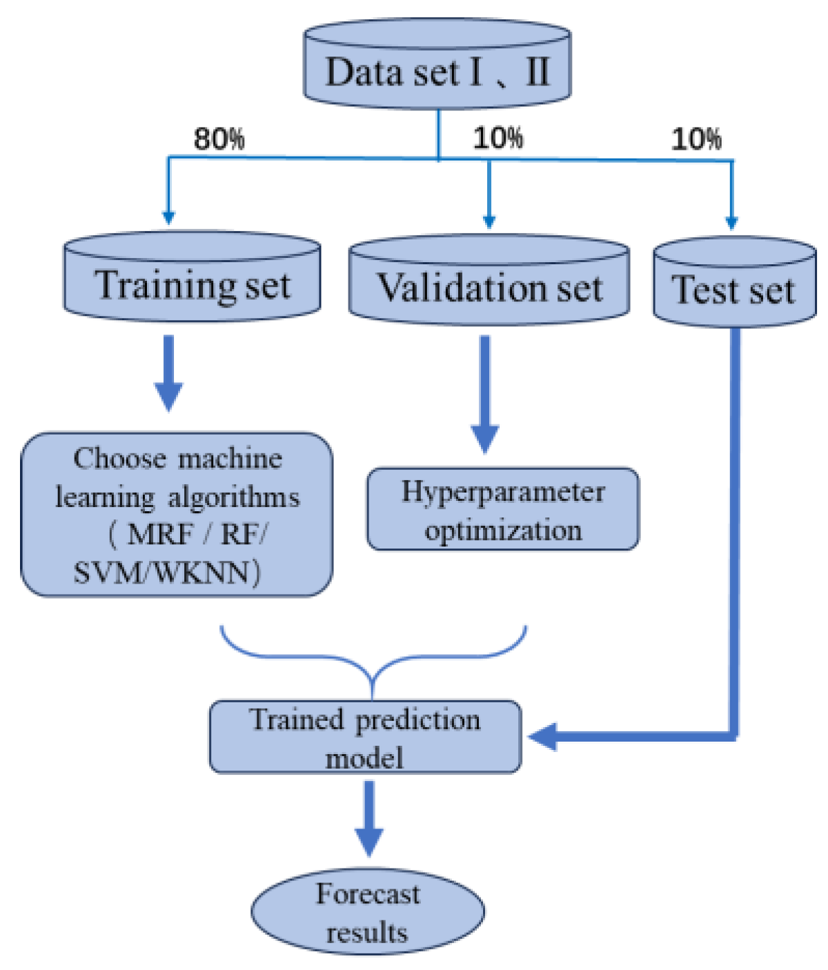
We took 80% of the dataset as the training set, 10% as the validation set, and 10% as the test set. The training set ranged from 1 January 2012 to 9 December 2021 (2415 days); the validation set ranged from 10 December 2021 to 10 March 2023 (302 days); and the test set ranged from 11 March 2023 to 11 June 2024 (302 days). The MRF, RF, SVM, and WKNN algorithms were used to build prediction models on the training set. The hyperparameters of the different models were optimized to obtain trained prediction models.

To identify the most influential predictors among the 26 candidate features, a five-fold cross-validated stepwise regression was performed on the combined training and validation dataset. In each fold, four subsets were used for model fitting and evaluated using the Akaike Information Criterion (AIC). The model with the minimum AIC was selected, and its retained variables were adopted as the final input features. Consequently, 16 significant predictors were identified: SMA(10), WMA(10), WR(6), RSI(6), RSI(12), AD, MTM(10), Stochastic D, ROC(12), BIAS(10), BIAS(15), MACD(9), CCI, MA(5), Closing Price, and ROC(1).

To compare the performance improvement of the prediction models produced by stepwise regression analysis, two datasets were used: the original dataset with 26 indicators and the dataset with 16 indicators selected by stepwise regression. The test samples from both datasets were input into the trained prediction models, and the prediction results for each test sample were output. The general process of constructing the prediction models in this study is shown in Figure 1. In Figure 1, the original dataset containing all 26 indicators is denoted as Dataset I, while the dataset comprising the 16 selected indicators is referred to as Dataset II.

2.5. Model Evaluation Metrics

To intuitively measure the ability of different prediction models to recognize the trend of the CSI 300 stock index, we establish the confusion matrix and introduce the four metrics of accuracy, precision, recall, and F₁ score to evaluate the model’s predictive capability. The calculation methods for these metrics are:

$$Accuracy={\displaystyle \frac{TP+TN}{TP+TN+FP+FN}},Precision={\displaystyle \frac{TP}{TP+FP}},Recall={\displaystyle \frac{TP}{TP+FN}},{\mathrm{F}}_{1}score={\displaystyle \frac{2TP}{2TP+FN+FP}}$$

(15)

where TP represents the number of correctly predicted upward samples, TN represents the number of correctly predicted downward samples, FP represents the number of downward samples incorrectly predicted as upward, and FN represents the number of upward samples incorrectly predicted as downward.

3. Results

3.1. Experimental Environment and Hyperparameter Settings

The experiments were conducted using the R 4.3.0 [28] language on a personal computer with the following specifications: Nvidia 3060 Laptop GPU (6 GB), manufactured by NVIDIA Corporation, Santa Clara, CA, USA, and an Intel Core i9-12900H @ 2.50 GHz CPU, manufactured by Intel Corporation, Santa Clara, CA, USA. The RF and MRF prediction models were established using the “randomForest.default” function from the R package “randomForest”. The full configuration details, resampling scheme, and implementation scripts are provided in the Supplementary Materials (Supplementary Folders S2 and S3).

The RF model has two important hyperparameters: the number of classifiers (ntree), i.e., the number of decision trees, and the maximum number of features (mtry). The maximum number of features controls the number of variables selected when splitting nodes, and thus determines the growth pattern of the decision trees. The MRF model includes these hyperparameters as well as the number of scales ${\sigma }_b^2,b=1,2,\cdots ,B$, which is the number of sample sizes $n_b,b=1,2,\cdots ,B$ during the resampling. According to the research experience of the literature [23], this value is typically around 10. For this study, we set $B$= 10.

For the SVM, the Gaussian kernel function was chosen. This has a parameter $\gamma$ that affects the data distribution in the new feature space. The penalty coefficient C also requires tuning.

For the WKNN, the hyperparameters are the distance function (distance), weight (weight), and number of neighbors $k$. The Euclidean distance was used for the distance function and we set distance = 2, with rectangular, triangular, and Gaussian kernels used for the weights. The number of neighbors was tuned during model optimization. The parameter ranges considered for the four models considered in this study are presented in

Table 2. Selection range of hyperparameters for different prediction models.

Prediction Model	Hyperparameter	Interpretation of Hyperparameter	Range of Hyperparameter
RF& MRF	ntree	number of classifiers	[100, 1000], by = 100
	mtry	maximum number of features	[1, i], by = 4, i = 16 or 26
SVM	kernel	kernel function	Gaussian kernel function
	C	penalty coefficient	{0.001,0.01,0.1,1,5,10,100,1000}
	$\gamma$	parameters for nonlinear kernel functions	[0.1, 2], by = 0.1
WKNN	distance	distance function	2
	weight	weight	{rectangular, triangular, Gaussian}
	$k$	number of nearest neighbors	[1, 20], by = 1

Note: For dataset I, i = 26, and for dataset II, i = 16.

.

A grid search was used for hyperparameter tuning in these complex parameter spaces. This method divides the parameter space into a grid and searches all points to find the optimal parameters. For this study, the hyperparameters were optimized in two steps: (i) training the model with the training set and (ii) improving the generalization ability of the model with the validation set to detect and adjust for overfitting.

Using the hyperparameter selection method described above, the optimal hyperparameter combinations for the four models on the different datasets were obtained using the R 4.3.0 software for statistical analysis. The results are presented in

Table 3. Hyperparameter selection for different machine learning models.

Prediction Model	Hyperparameter	Interpretation of Hyperparameter	Value of Hyperparameter (Dataset I)	Value of Hyperparameter (Dataset II)
RF	ntree	number of classifiers	600	900
	mtry	maximum number of features	21	5
MRF	ntree	number of classifiers	800	100
	mtry	maximum number of features	13	5
SVM	kernel	kernel function	Gaussian kernel function	Gaussian kernel function
	C	penalty coefficient	5	5
	$\gamma$	parameters for nonlinear kernel functions	0.1	0.1
WKNN	distance	distance function	2	2
	weight	weight	triangular	triangular
	$k$	number of nearest neighbors	20	14

.

3.2. Empirical Results Analysis

3.2.1. Comparison of Prediction Performance Based on Test Set I

According to the dataset division rules given in Section 2.5, prediction models were constructed on the training and validation sets, and the confusion matrix obtained on the test set was used to evaluate the prediction results of the different models. The results in

Table 4. Confusion matrix of different prediction models (test set I).

Prediction Model	Actual Category	Prediction Category
		0-“Downward”	1-“Upward”
MRF	0-“downward”	135	31
	1-“upward”	30	106
RF	0-“downward”	129	37
	1-“upward”	29	107
SVM	0-“downward”	118	48
	1-“upward”	23	113
WKNN	0-“downward”	101	65
	1-“upward”	27	109

Note: 0 represents (0 or −1).

indicate that, using test set I with all 26 indicators directly as input variables, the machine learning models exhibit different abilities to recognize “upward” and “downward” samples. The MRF and RF models have stronger recognition capabilities for downward samples, the SVM has more balanced recognition capabilities for both types of samples, and the WKNN model has stronger recognition capabilities for upward samples. Based on the confusion matrices of the different prediction models, the accuracy, precision, recall, and F₁ score were calculated. The results are given in

Table 5. Evaluation metrics for different prediction models (test set I).

Prediction Model	Accuracy	Precision	Recall	F1 Score
MRF	0.7980	0.7737	0.7794	0.7766
RF	0.7815	0.7431	0.7868	0.7643
SVM	0.7649	0.7019	0.8309	0.7609
WKNN	0.6954	0.6264	0.8015	0.7032

.

First, the MRF model demonstrates the best overall performance, with an accuracy of 0.7980 and an F₁ score of 0.7766, indicating the highest recognition ability for different types of samples. The proposed model also has the highest precision at 0.7737, meaning that 77.37% of the samples predicted as upward are actually upward. The recall is 0.7794, indicating that the model correctly predicted 77.94% of the actual upward samples. In contrast, the SVM achieves the highest recall of 0.8309, indicating that it is the least likely to misclassify upward samples as downward. The RF model performs similarly to the SVM, with an accuracy of 0.7815, but with a lower recall of 0.7868, suggesting it is less effective than the SVM in correctly identifying all upward samples. The WKNN model gives the worst results across all metrics, reflecting its inadequacy in adapting to the current dataset.

By plotting the ROC curves and calculating the AUC values, the predictive capabilities of the models can also be intuitively compared, as shown in Figure 2. On Test Set I, the MRF model achieves an AUC value of 0.8747, which is higher than that of the RF and WKNN models but slightly lower than that of the SVM model. This indicates that both the MRF and SVM models yield relatively strong predictive performance in the context of stock index movement forecasting.

3.2.2. Comparison of Prediction Performance Based on Test Set II

Table 6. Confusion matrix of different prediction models (test set II).

Prediction Model	Actual Category	Prediction Category
		0-“Downward”	1-“Upward”
MRF	0-“downward”	135	31
	1-“upward”	25	111
RF	0-“downward”	130	36
	1-“upward”	27	109
SVM	0-“downward”	143	23
	1-“upward”	49	87
WKNN	0-“downward”	98	68
	1-“upward”	29	107

Note: 0 represents (0 or −1).

suggests that using the 16 indicators selected through stepwise regression analysis as input variables improves the prediction performance. At this stage, each prediction model exhibits stronger recognition capabilities for upward samples.

The evaluation metrics for the different prediction models on test set II are presented in

Table 7. Evaluation metrics for different prediction models (test set II).

Prediction Model	Accuracy	Precision	Recall	F1 Score
MRF	0.8146	0.7817	0.8162	0.7986
RF	0.7914	0.7517	0.8015	0.7758
SVM	0.7615	0.7909	0.6397	0.7073
WKNN	0.6788	0.6114	0.7868	0.6881

. Table 7 compares the performance of different prediction models on Test Set II. Among all models, the MRF model achieves the best overall performance, with the highest accuracy (0.8146), recall (0.8162), and F₁ score (0.7986). The RF model ranks second across most metrics, while SVM shows relatively high precision but lower recall. The WKNN model performs the weakest, with the lowest scores in all evaluation metrics. Overall, the MRF model per- forms better on test set II than on test set I, demonstrating strong overall performance and accurate recognition of downward samples.

Comprehensive analysis of the evaluation metrics achieved on both test sets demonstrates that, while it may not always be the best in terms of individual metrics, the MRF model exhibits superior performance when considering all evaluation metrics together, achieving a good balance. This balance is reflected in its high accuracy in judging upward samples and relatively accurate identification of downward samples, ensuring the stability and accuracy of the prediction model. These characteristics are crucial for many practical applications.

As shown in Figure 3, the ROC curves of different prediction models on Test Set II are presented. The MRF model achieves an AUC value of 0.8727, which is higher than that of the SVM and WKNN models but slightly lower than that of the RF model. This suggests that incorporating stepwise regression analysis can effectively enhance the performance of the MRF model in forecasting the CSI 300 stock index.

3.3. Comparison of Model Computational Efficiency

This section compares the runtimes of the different algorithms to demonstrate the practicality of the MRF algorithm from the perspective of actual operability.

Table 8. Runtimes of different models on training and test sets.

Prediction Model	Running Time (s)
	training set I	training set II	test set I	test set II
MRF	1.3315	0.8415	0.2775	0.2440
RF	0.3298	0.2306	0.0053	0.0050
SVM	1.6135	1.5114	0.0213	0.0157
WKNN	0.2002	0.1313	0.0255	0.0205

lists the runtimes on the training and test sets. The MRF model has a shorter runtime on the different training sets than SVM, but requires longer for training than RF and WKNN. Additionally, the proposed MRF model has the longest runtime on the different test sets. However, the overall runtime difference is less than 1 s. This difference is caused by the multiple resampling processes during MRF model training, which require the model to handle more data. During the prediction stage, the MRF model adjusts the $BP$ using a relatively complex calculation process, leading to increased runtime on the test set. In practical applications, the choice of algorithm should consider runtime, accuracy, and stability. When computational resources are sufficient, algorithms with slightly longer runtimes but higher accuracy are preferable. Therefore, the MRF model developed in this study has practical application value.

4. Discussion and Conclusions

Comparing this study with related research demonstrates the effectiveness of the MRF model based on stepwise regression analysis for predicting the trend of the CSI 300 stock index.

For instance, Wang and Zhu [29] developed a hybrid deep learning model that integrates financial sentiment scores and news flow features to predict stock index movements. Their model achieved an accuracy, precision, recall rate and F₁ score of 80.07%, 80.07%, 80.07% and 80.06%, respectively, on a test set covering the period from October 26, 2020 to December 31, 2021 (291 days). In comparison, on Test Set II covering March 11, 2023 to June 11, 2024 (302 days), the proposed MRF model achieved an accuracy of 81.46%, precision of 78.17%, recall of 81.62%, and F₁ score of 79.86%, accuracy and recall of which exceed the metrics reported by Wang and Zhu. This suggests that the MRF model not only captures temporal and structural patterns in financial time series more effectively, but also provides more statistically reliable prediction confidence through the integration of multiscale bootstrap-based p-value correction, even without relying on external text-based sentiment indicators.

Two test sets based on the CSI 300 stock index are used to evaluate the predictive performance of the proposed MRF model. In Test Set I, the accuracy, precision, recall and F₁ score reached 79.80%, 77.37%, 77.94% and 77.66%, respectively, while in Test Set II, the accuracy and precision improved to 81.46% and 78.17%, with recall and F₁ score reaching 81.62% and 79.86%, respectively. Compared with existing models such as RF, SVM and WKNN, the proposed MRF model achieves superior performance across multiple evaluation metrics, particularly in terms of accuracy and precision. These improvements stem from two key innovations: (i) the introduction of multiscale bootstrap resampling, which increases the diversity and robustness of the ensemble learning framework; and (ii) the incorporation of an unbiased p-value with third-order accuracy during prediction, enhancing classification reliability beyond traditional majority voting schemes. Additionally, stepwise regression contributes further by eliminating redundant variables and enhancing the relevance of input features, thereby improving model interpretability and reducing overfitting. Overall, the combination of statistical feature selection with an advanced ensemble learning framework offers a practical and effective approach for forecasting complex financial time series. From a theoretical standpoint, this work extends the conventional random forest framework by integrating the multiscale bootstrap method proposed by Shimodaira [18,19,20,21] into ensemble learning. The resulting MRF model formally incorporates resampling-scale-dependent bootstrap probabilities and corrects classification bias via third-order p-value extrapolation. This represents a novel application of statistical hypothesis testing techniques in supervised machine learning, offering a mathematically grounded approach to improve voting-based classifiers. The model bridges statistical inference and ensemble learning, providing a new direction for future research in robust and interpretable machine learning algorithms. It should be noted that the MRF model proposed in this paper is limited to predicting classification problems, such as determining whether future stock prices will rise or fall. At present, it cannot be applied to continuous variables. However, the conventional random forest does not have this limitation and can be used for regression problems.