Abstract
In numerical analysis, the Boole’s formula serves as a pivotal tool for approximating definite integrals. The approximation of the definite integrals has a big role in numerical methods for differential equations; in particular, in the finite volume method, we need to use the best approximation of the integrals to obtain better results. This paper presents a rigorous proof of integral inequalities for first-time differentiable s-convex functions in the second sense. This paper has two main goals. The first is that the use of s-convex function extends the results for convex functions which cover a large class of functions and the second is the best approximation. To prove the main inequalities, we drive integral identity for differentiable functions. Then, with the help of this identity, we prove the error bounds of Boole’s formula for differentiable s-convex functions in the second sense. Some new midpoint-type inequalities for generalized convex functions are also given which can help us in finding better error bounds for midpoint integration formulas compared to the existing ones. Moreover, we provide some applications to quadrature formulas and special means for the real numbers of these newly established inequalities. Furthermore, we present numerical examples and computational analysis that show that these newly established inequalities are numerically valid.
Keywords:
Boole’s formula-type inequality; modified convex function; quadrature formulae; midpoint formula; error bounds MSC:
26D10; 26D15; 26A51
1. Introduction
The concept of numerical integration was formally introduced in 1915 in a publication titled A Course in Interpolation and Numerical Integration for the Mathematical Laboratory by David Gibb [1]. In recent decades, numerical integration has become an essential component of scientific computing, engineering, and data analysis. The term quadrature is a traditional mathematical expression for finding areas. By constructing various interpolating polynomials, a broad class of quadrature rules can be derived. One of the simplest methods assumes the interpolating function to be constant (a zero-degree polynomial), known as the midpoint or rectangle rule. When the interpolating function is linear, the corresponding method is called the trapezoidal rule. If the interpolating polynomial is of the second degree, the resulting method is Simpson’s rule, named after mathematician Thomas Simpson (1710–1761), whose simplest form is known as Simpson’s rule.
To achieve higher accuracy with smaller error bounds, a more advanced form known as the Boole rule is used, also known as Simpson’s or third Simpson rule. Named after George Boole, this method extends Simpson’s approach by using a higher-degree polynomial, thereby providing improved precision in the numerical approximation of integrals.
where is an error term. To know more about numerical integration and its applications one can refer to [2]. The error bound for Boole’s rule approximation is described as
Convexity is a property of a function where any line segment joining two points on its graph will always lie above or on the graph. Convexity plays a vital role in calculus, optimization, and mathematical analysis. Additional results and related inequalities for convex functions are discussed in [3,4,5,6]. The formal definition is as follows:
Definition 1
([7]). A function is said to be convex if
for each value of .
Convex functions are involved in important mathematical inequalities known as Hermite–Hadamard-type inequalities, which are expressed as
Theorem 1.
For a convex function the interval . Then, we have
The aforementioned inequalities likewise apply to concave functions, although they work in the other way. Kirmaci [8] introduced the following midpoint-type inequality along with its error bounds for differentiable convex mappings, one of which is as follows:
Theorem 2.
Let be a differentiable mapping on ; then, we have
In the literature, a Simpson-type inequality is outlined as follows:
Theorem 3.
Let be a four-times differentiable mapping on ; then, we have
where .
The study of error bounds for numerical quadrature formulas has attracted considerable attention in the literature. In their pioneering work, Dragomir and Agarwal [9] extended the classical inequality and obtained sharp estimates for the error term of the trapezoidal rule when the integrand is assumed to be a differentiable convex function. Building upon this framework, Kirmaci [8] focused on the midpoint rule and established corresponding error bounds under the same convexity setting. These initial contributions opened up a new direction for research, encouraging many scholars to investigate error estimates for various quadrature rules under broader assumptions and by means of different analytical tools. Subsequently, Alomari and Dragomir [10,11] considered the Simpson formula and derived error bounds not only for convex functions but also for the wider class of generalized convex functions. Their work also highlighted some practical applications, which emphasized the utility of such results. Parallel to these studies, other authors extended Simpson-type inequalities to multivariate settings. For example, in [12,13], the error bounds for Simpson’s rule were analyzed for functions of two variables, thereby enriching the scope of quadrature error analysis in higher dimensions. Furthermore, Du [14] utilized a general form of convexity in order to establish new estimates for Simpson’s formula, broadening the applicability of such inequalities beyond the standard convex case.
In a more comprehensive sense, a variety of fundamental inequalities, including those of a Hermite–Hadamard, Ostrowski, midpoint, Simpson, and trapezoidal type, provide the theoretical basis for deriving error bounds of integration formulas. Numerous results of this nature can be found in the works of [15,16,17,18,19,20], where these classical inequalities are employed as essential tools to analyze and refine the accuracy of numerical integration methods.
In 1979, Breckner introduced the notion of generalized convex functions [21], marking a substantial advancement in the field of mathematical analysis. This work was later expanded upon by Hudzik and collaborators [22], who investigated the concept of s-convexity in the first sense. Pycia [23] subsequently provided rigorous demonstrations of Breckner’s propositions in 2001. Analytical investigations have established that for a parameter , the condition of s-convexity in the second sense imposes a more restrictive and potent constraint than classical convexity, frequently producing sharper and more refined results. Furthermore, this framework provides a natural generalization of conventional convex functions, as the standard case is recovered by setting . The class is formally characterized in the following manner:
Definition 2
In [24], the Hermite–Hadamard inequality for s-convex functions is stated as
Theorem 4.
If is an s-convex function in the second sense, where , let , If , then the following inequality holds:
Refer to [25,26,27,28,29,30,31,32] for more recent results and insights regarding Hadamard’s inequality.
The main motivation for using s-convexity is that it broadens the class of admissible functions for which integral inequalities can be established. Many functions that fail to satisfy the classical convexity condition may still satisfy the s-convexity condition for some . This makes it possible to derive more general and sharper inequalities that depend on the parameter s. The key advantages of employing s-convexity are summarized as follows:
- It provides a unified framework that includes the classical convex case as a special instance when ;
- The parameter s offers flexibility to obtain sharper and more refined inequality bounds;
- It allows the extension of classical results such as Hermite–Hadamard-, Simpson-, and Boole-type inequalities and other Newton–Cotes formulae-type inequalities to a broader class of functions;
- The derived inequalities often yield improved error bounds in numerical integration and approximation theory.
Motivated by recent studies, a new identity for differentiable mappings based on generalized convexity is established. This identity is then used to derive Boole-type inequalities for differentiable convex functions, along with their applications. Numerical examples are presented to illustrate the validity of the results. This generalization unifies previous results and deepens the understanding of Boole-type inequalities for numerical integration and error estimation.
The structure of the paper is as follows. Section 2 presents the main results for differentiable s-convex functions in the second sense. Applications to numerical integration and special means are given in Section 3. Section 4 provides computational examples illustrating the new inequalities. Concluding remarks with future directions are given in Section 5.
2. Boole-Type Inequality for Modified Convex Function
We rely on the following Lemma to establish our main theorems for s- convex functions.
Lemma 1.
Consider to be a differentiable function whose derivative is continuous and Then, the subsequent equality is satisfied:
Proof.
Theorem 5.
Assume that the premises established in Lemma 1 are fulfilled. If is s-convex on , for some fixed , then the following inequality holds:
Proof.
From Lemma 1 and taking the modulus, we obtain
Now, using the s-convexity of in the second sense, we have
Here, we used the following equalities:
Putting the above calculations into inequality (11), we then obtain
Thus, the proof of Theorem 5 has been finalized. □
Corollary 1.
By setting in Theorem 5, the following inequality holds:
Corollary 2.
In Theorem 5, if then we have the following new midpoint-type inequality for the s-convex function:
Corollary 3.
By setting in Corollary 2, we obtain
Remark 1.
Theorem 6.
Assume that the premises established in Lemma 1 are fulfilled. If is s-convex on , for some fixed and , then the following inequality holds:
where .
Proof.
Corollary 4.
Setting in Theorem 6, we have
The new midpoint-type inequality in terms of the first derivative is observed in the following result:
Corollary 5.
In Theorem 6, if then we have the following midpoint-type inequality for the s-convex function:
Corollary 6.
In Corollary 5, setting we have
Theorem 7.
Assume that the premises established in Lemma 1 are fulfilled. If is s-convex on , for some fixed and then the following inequality holds:
3. Applications
This section presents several applications of the newly established results to numerical quadrature formulas.
3.1. Application to Quadrature Formulas
Consider a partition of the interval , defined by , and let . The associated Boole’s quadrature formula is given by
The classical error analysis for this quadrature rule states that if , then the integral can be expressed as
with the remainder term satisfying the error bound
where . We note that the bound (32) is proportional to , as required for the dimensional consistency and linearity of the error functional.
However, this classical error estimate is inapplicable if lacks a sixth derivative or if is unbounded. The following propositions provide alternative error bounds for the remainder term based on properties of the first derivative.
Proposition 1.
Assume the conditions of Lemma 1 hold. If is convex on , then for any partition Υ of , the following inequality holds:
Proof.
Applying Corollary 1 to each subinterval for yields:
Summing the inequality (34) over all subintervals and employing the triangle inequality, together with the convexity of , we obtain
which completes the proof. □
Remark 2.
One can similarly derive an approximation based on Theorems 6 and 7, respectively; the details are omitted for brevity and are left to the interested reader.
3.2. Application to the Midpoint Formula
Consider a partition of the interval , defined by . The composite midpoint rule for numerical integration is given by
A standard result states that if is a twice-differentiable function, such that its second derivative exists on and is bounded, i.e., , then the integral can be expressed as
where the error term satisfies the bound
This classical error estimate requires the existence and boundedness of the second derivative. The following result provides an alternative error bound for the remainder term in terms of the first derivative, offering an improvement over previous results in certain contexts.
Proposition 2.
Assume that the conditions of Lemma 1 are satisfied. If is a convex function on , then for any partition of , the following inequality holds:
Proof.
Applying Corollary 3 to each subinterval for yields the following local error estimate:
Summing the inequality (39) over all subintervals and applying the triangle inequality, we obtain the global error bound:
which completes the proof. □
Remark 3.
The estimations for midpoint-type inequality given in this work provided better bounds compared to the estimation proved in [8].
3.3. Application to Special Means
Let and . We define a function as
If and , then (see [22]). Hence, for and , we have a function defined by , which belongs to .
In [22], the following result is given. Let be a non-decreasing and s-convex function on , and let be a non-negative convex function on J. Then the composition is s-convex on J.
A direct result of the previous finding can be stated as follows:
Corollary 7.
Suppose is a non-negative convex function on I, then is s-convex on
We shall consider the following special means. For arbitrary real numbers (), we have the following:
The arithmetic mean:
The harmonic mean:
The logarithm mean:
The p-logarithmic mean: and It is well-known that is monotonic non-decreasing over , with and . In particular, we have the following inequality .
Based on the outcomes presented in Section 2, we establish new inequalities for the means mentioned above.
4. Numerical Examples
In this section, a comprehensive numerical investigation is carried out to confirm the validity and efficiency of the newly established results. Several computational experiments are presented to highlight the applicability of the proposed inequalities, especially for the approximation of integrals involving differentiable s-convex functions. To better illustrate the outcomes, three-dimensional graphical models are employed, providing clear insights into the numerical behavior of the derived inequalities. These visual demonstrations play a crucial role in verifying the accuracy and practical significance of the theoretical contributions.
Example 1.
Let be a function defined by . Then by applying inequality (10) to the function , the left-hand side of inequality (10) for is
and the right-hand side of inequality (10) for is
From Equations (42) and (43), it is clear that the left-hand side is less than the right-hand side
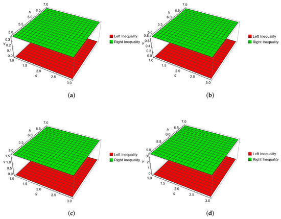
This demonstrates that the inequality (10) is valid. A visual confirmation of this result is provided in Figure 1.
Figure 1.
The graphical evidence presented in Figures (a–d) demonstrates that for every , the value of the left-hand side of inequality (10) is strictly bounded below by its right-hand side. This observation provides empirical confirmation of the result stated in Theorem 5.
Example 2.
Let be a function defined by . Then by applying inequality (10) to the function , the left-hand side of inequality (10) for is
and the right-hand side of inequality (10) for is
From Equations (44) and (45), it is clear that the left-hand side is less than the right-hand side
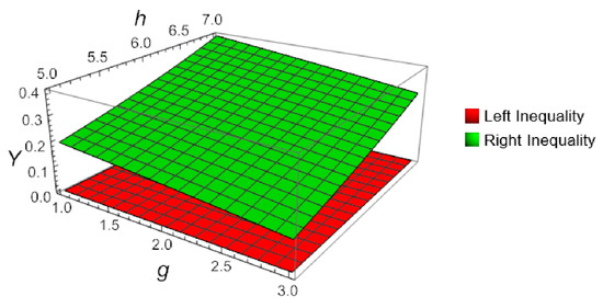
This observation serves as a numerical verification of inequality (10). A visual confirmation of this result is provided in Figure 2.
Figure 2.
Three-dimensional plot for Theorem 5 in Example 2, when , , and , computed and plotted with Mathematica.
Example 3.
Let be a function defined by . Then by applying inequality (10) to the function , the left-hand side of inequality (10) for is
and the right-hand side of inequality (10) for is
From Equations (46) and (47), it is clear that the left-hand side is less than the right-hand side
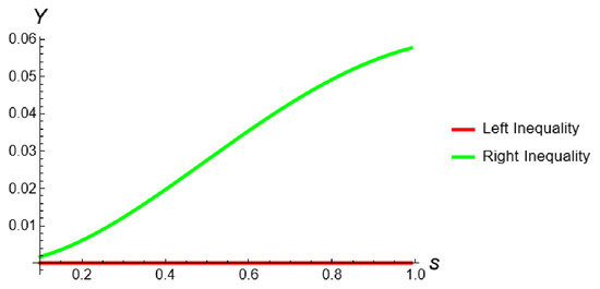
This demonstrates that the inequality (10) is valid. A visual confirmation of this result is provided in Figure 3.
Figure 3.
Two-dimensional plot for Theorem 5 in Example 3, when , and , computed and plotted with Mathematica.
Example 4.
Let be a function defined by and . Then by applying inequality (14) to the function , the right-hand side of inequality (14) for is
From Equations (42) and (48), it is clear that the left-hand side is less than the right-hand side
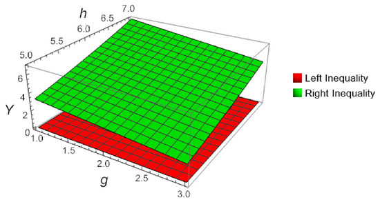
This observation serves as a numerical verification of inequality (14). A visual confirmation of this result is provided in Figure 4.
Figure 4.
Three-dimensional plot for Theorem 6 in Example 4, when , , and , computed and plotted with Mathematica.
Example 5.
Let be a function defined by and . Then by applying inequality (24) to the function , then the left-hand side of inequality (24) for is
and the right-hand side of inequality (24) for is
From Equations (49) and (50), it is clear that the left-hand side is less than the right-hand side
This observation serves as a numerical verification of inequality (24).
5. Conclusions
The main focus of this study was to establish new Boole’s formula-type inequalities for single-time differentiable s-convex functions in the second sense. By employing an integral identity, several inequalities were derived that extend the classical framework and provide improved bounds for both Boole’s and midpoint formulas. The findings indicate that the proposed error estimates outperform some existing results, with s-convexity offering tighter approximations compared to standard convexity. In particular, the analysis demonstrates that as the parameter s varies, the obtained bounds surpass those of the classical case , while the error tends to diminish as . The study further validates its results through applications to quadrature formulas and special means of real numbers, supported by numerical examples, computational analysis, and graphical models. Evidence from Table 1 and Table 2 confirms the effectiveness of the proposed approach for generalized convex functions. These contributions enrich approximation theory, real analysis, and the study of functional inequalities by providing more precise error estimates for polynomial and functional approximations.

Table 1.
Computational analysis between the left-hand and the right-hand sides of inequality (10) for discretization of “s” in Example 1.
Table 2.
Computational analysis between the left-hand and the right-hand sides of inequality (10) for discretization of “s” in Example 2.
Looking ahead, this research can be extended by incorporating q-calculus, fractional calculus, higher-order derivatives, multidimensional frameworks, and alternative convexity structures. The outcomes presented here highlight the significance of Boole’s formula-type inequalities as powerful tools in the advancement of integral inequality theory.
Author Contributions
Conceptualization, A.M.; formal analysis, T.A., A.M., H.E. and L.C.; funding acquisition, L.C.; investigation, T.A., A.M., M.A.A. and L.C.; methodology, T.A., A.M., H.E. and M.A.A.; software, A.M.; supervision, M.A.A.; validation, T.A., A.M., H.E., M.A.A. and L.C.; visualization, T.A., A.M., H.E. and M.A.A.; writing—original draft, T.A. and A.M.; writing—review and editing, T.A., A.M., H.E., M.A.A. and L.C. All authors have read and agreed to the published version of the manuscript.
Funding
Princess Nourah bint Abdulrahman University Researchers Supporting Project number (PNURSP2025R747), Princess Nourah bint Abdulrahman University, Riyadh, Saudi Arabia.
Data Availability Statement
The original contributions presented in this study are included in the article. Further inquiries can be directed to the corresponding author.
Acknowledgments
Princess Nourah bint Abdulrahman University Researchers Supporting Project number (PNURSP2025R747), Princess Nourah bint Abdulrahman University, Riyadh, Saudi Arabia.
Conflicts of Interest
We declare that we have no conflicts of interest in this work.
References
- Gibb, D. A Course in Interpolation and Numerical Integration for the Mathematical Laboratory; G. Bell & Sons, Limited: London, UK, 1915. [Google Scholar]
- Leader, J.J. Numerical Analysis and Scientific Computation; Chapman and Hall/CRC: Boca Raton, FL, USA, 2022. [Google Scholar]
- Ali, M.A.; Kara, H.; Tariboon, J.; Asawasamrit, S.; Budak, H.; Hezenci, F. Some new Simpson’s-formula-type inequalities for twice-differentiable convex functions via generalized fractional operators. Symmetry 2021, 13, 2249. [Google Scholar] [CrossRef]
- Ali, M.A.; Fečkan, M.; Mateen, A. Study of quantum Ostrowski’s-type inequalities for differentiable convex functions. Ukr. Math. J. 2023, 75, 7–27. [Google Scholar] [CrossRef]
- Vivas-Cortez, M.J.; Ali, M.A.; Qaisar, S.; Sial, I.B.; Jansem, S.; Mateen, A. On some new Simpson’s formula type inequalities for convex functions in post-quantum calculus. Symmetry 2021, 13, 2419. [Google Scholar] [CrossRef]
- Mateen, A.; Zhang, Z.; Ali, M.A. Some Milne’s rule type inequalities for convex functions with their computational analysis on quantum calculus. Filomat 2024, 38, 3329–3345. [Google Scholar] [CrossRef]
- Dwilewicz, R.J. A short history of convexity. Differ.-Geom.-Dyn. Syst. 2009, 11, 112–129. [Google Scholar]
- Kirmaci, U.S. Inequalities for differentiable mappings and applications to special means of real numbers and to midpoint formula. Appl. Math. Comput. 2004, 147, 137–146. [Google Scholar] [CrossRef]
- Dragomir, S.S.; Agarwal, R.P. Two inequalities for differentiable mappings and applications to special means of real numbers and to trapezoidal formula. Appl. Math. Lett. 1998, 11, 91–95. [Google Scholar] [CrossRef]
- Alomari, M.; Darus, M.; Dragomir, S.S. New inequalities of Simpson’s type for s-convex functions with applications. Res. Rep. Collect. 2009, 12, 50. [Google Scholar]
- Dragomir, S.S.; Agarwal, R.P.; Cerone, P. On Simpson’s inequality and applications. RGMIA Res. Rep. Collect. 2012, 2, 75. [Google Scholar] [CrossRef]
- Sarikaya, M.Z.; Set, E.; Özdemir, M.E. On new inequalities of Simpson’s type for convex functions. RGMIA Res. Rep. Collect. 2010, 13, 25. [Google Scholar] [CrossRef]
- Özdemir, M.E.; Akdemir, A.O.; Kavurmaci, H.; Avci, M. On the Simpson’s inequality for co-ordinated convex functions. Turk. J. Math. Anal. Number Theory 2014, 2, 165–169. [Google Scholar] [CrossRef]
- Du, T.; Li, Y.; Yang, Z. A generalization of Simpson’s inequality via differentiable mappings using extended (s,m)-convex functions. Appl. Math. Comput. 2017, 293, 358–369. [Google Scholar] [CrossRef]
- Sarikaya, M.Z.; Set, E.; Yaldiz, H.; Başak, N. Hermite–Hadamard’s inequalities for fractional integrals and related fractional inequalities. Math. Comput. Model. 2013, 57, 2403–2407. [Google Scholar] [CrossRef]
- İşcan, İ.; Wu, S. Hermite–Hadamard type inequalities for harmonically convex functions via fractional integrals. Appl. Math. Comput. 2014, 238, 237–244. [Google Scholar] [CrossRef]
- Sarikaya, M.Z.; Yildirim, H. On Hermite-Hadamard type inequalities for Riemann-Liouville fractional integrals. Miskolc Math. Notes 2016, 17, 1049–1059. [Google Scholar] [CrossRef]
- Sarikaya, M.Z.; Set, E.; Ozdemir, M.E. On new inequalities of Simpson’s type for s-convex functions. Comput. Math. Appl. 2010, 60, 2191–2199. [Google Scholar] [CrossRef]
- Chen, J.; Huang, X. Some new inequalities of Simpson’s type for s-convex functions via fractional integrals. Filomat 2017, 31, 4989–4997. [Google Scholar] [CrossRef]
- Budak, H.; Hezenci, F.; Kara, H. On parameterized inequalities of Ostrowski and Simpson type for convex functions via generalized fractional integrals. Math. Methods Appl. Sci. 2021, 44, 12522–12536. [Google Scholar] [CrossRef]
- Breckner, W.W. Stetigkeitsaussagen für eine klasse verallgemeinerter konvexer funktionen in topologischen linearen räumen. Publ. De L’Institut MathéMatique 1978, 23, 13–20. [Google Scholar]
- Hudzik, H.; Maligranda, L. Some remarks on s-convex functions. Aequationes Math. 1994, 48, 100–111. [Google Scholar] [CrossRef]
- Pycia, M. A direct proof of the s-Hölder continuity of Breckner s-convex functions. Aequationes Math. 2001, 61, 128–130. [Google Scholar] [CrossRef]
- Dragomir, S.S.; Fitzpatrick, S. The Hadamard’s inequality for s-convex functions in the second sense. Demonstr. Math. 1999, 32, 687–696. [Google Scholar]
- Kirmaci, U.S.; Bakula, M.K.; Özdemir, M.E.; Pečarić, J. Hadamard-type inequalities for s-convex functions. Appl. Math. Comput. 2007, 193, 26–35. [Google Scholar] [CrossRef]
- Alomari, M.; Darus, M.; Dragomir, S.S. Inequalities of Hermite-Hadamard’s type for functions whose derivatives absolute values are quasi-convex. Res. Rep. Collect. 2009, 12, 1. [Google Scholar]
- Alomari, M.; Darus, M.; Kirmaci, U.S. Refinements of Hadamard-type inequalities for quasi-convex functions with applications to trapezoidal formula and to special means. Comput. Math. Appl. 2010, 59, 225–232. [Google Scholar] [CrossRef]
- Kashuri, A.; Liko, R. Fractional trapezium type inequalities for twice differentiable preinvex functions and their applications. Int. J. Optim. Control. Theor. Appl. 2020, 10, 226–236. [Google Scholar] [CrossRef]
- Yildiz, Ç.; Yergöz, B.; Yergöz, A. On new general inequalities for s-convex functions and their applications. J. Inequalities Appl. 2023, 2023, 11. [Google Scholar] [CrossRef]
- Sezer, S. The Hermite-Hadamard inequality for s-convex functions in the third sense. AIMS Math. 2021, 6, 7719–7732. [Google Scholar] [CrossRef]
- Barsam, H.; Ramezani, S.M.; Sayyari, Y. On the new Hermite–Hadamard type inequalities for s-convex functions. Afr. Mat. 2021, 32, 1355–1367. [Google Scholar] [CrossRef]
- Zhan, X.; Mateen, A.; Toseef, M.; Ali, M.A. Some Simpson- and Ostrowski-type integral inequalities for generalized convex functions in multiplicative calculus with their computational analysis. Mathematics 2024, 12, 1721. [Google Scholar] [CrossRef]


Disclaimer/Publisher’s Note: The statements, opinions and data contained in all publications are solely those of the individual author(s) and contributor(s) and not of MDPI and/or the editor(s). MDPI and/or the editor(s) disclaim responsibility for any injury to people or property resulting from any ideas, methods, instructions or products referred to in the content. |
© 2025 by the authors. Licensee MDPI, Basel, Switzerland. This article is an open access article distributed under the terms and conditions of the Creative Commons Attribution (CC BY) license (https://creativecommons.org/licenses/by/4.0/).