Abstract
Accurate estimation of probability distribution parameters is fundamental in frequency analyses of extreme hydrological and meteorological events. The reliability of such analyses largely depends on the estimation method adopted and on the availability of explicit relationships for parameter calculation. However, many parameter estimation methods are not yet implemented in specialized software, which limits their practical applicability. This study presents innovative explicit relationships for estimating the parameters of the Weibull distribution—one of the most widely used models in hydrology and environmental sciences—using the Known Moments method (K-moments). The proposed approximations, based on rational functions, enable the estimation of Weibull parameters (particularly the shape parameter) with admissible relative errors below 1%. The performance of the K-moments method was demonstrated through representative case studies from Romanian hydrology. The results show that the developed relationships significantly simplify the practical implementation of the Weibull distribution in frequency analysis using K-moments, ensuring both high accuracy and computational efficiency.
MSC:
62D05; 62F40; 62F07; 62P12; 62P30
1. Introduction
Frequency analysis of extreme events represents a cornerstone in hydrological design and risk assessment, supporting the dimensioning of hydraulic structures, flood mitigation systems, and water resource management strategies.
In the field of reliability engineering, methods for estimating the parameters of probability distributions have become essential tools for the probabilistic characterization of random variables that describe degradation processes, time-to-failure distributions, or residual strengths.
The reliability of such analyses depends not only on the quality of input data but also on the choice of probability distribution and the accuracy of its parameter estimation. In this context, a large variety of distributions—such as GEV, Pearson III, Log-Normal, Wakeby, generalized Pareto, Gumbel and Weibull—have been proposed to describe extreme flows, rainfall, or wind speeds [1,2,3]. Among these, the Weibull distribution has gained particular importance due to its flexibility and mathematical simplicity [4,5,6,7,8,9,10].
Traditional methods for parameter estimation, such as the method of moments, maximum likelihood, or L-moments, often require iterative numerical procedures or software packages that are not universally accessible. Moreover, many advanced distributions are not yet integrated into commercial or open-source hydrological programs, making their practical use difficult. The existence of explicit analytical relationships for parameter estimation can therefore greatly enhance both applicability and reproducibility, especially when quick or large-scale analyses are required.
The K-moments method [11,12], recently introduced as an alternative to classical L-moments, provides improved robustness to outliers and better numerical stability for small samples. Building upon this framework, the present study develops and validates explicit approximation formulas for the parameters of the Weibull distribution using rational expression, with estimation errors below 1%. In addition, the performance of the K-moments method was demonstrated through two representative case studies relevant to technical hydrology in Romania.
Other new elements presented in the manuscript include the approximate relationships for estimating the parameters of the Weibull distribution using the L-moments and MOM methods.
This manuscript contributes to expanding the toolbox of statistical parameter estimation in hydrological frequency analysis, by combining analytical simplicity, computational efficiency, and high accuracy within the K-moments theoretical framework.
2. Materials and Methods
If a random variable X follows a Weibull distribution, the probability density function with parameters, , and is defined by:
The complementary cumulative distribution function is:
The quantile function is:
2.1. Parameter Estimation—K-Moments
For a parametric model with parameters , the K-moments method estimates these parameters by imposing equality between the theoretical K-moments and the sample K-moments. For a three-parameter distribution, the orders moments (commonly 1, 2, 3 or 4) are [11,12]:
where
, represents the theoretical central (upper) K-moments of the distribution; , represents the annual probability of exceedance; , represents the arithmetic mean.
The K-moments for the sample are calculated using the following relations:
where
represents the empirical probability associated with the sample data. The combinatorial formula for Equation (5) is found in [11,12].
For the central moments:
, represents the sample expected value.
By ratios of these K-moments, the relations for K-coefficient of variation (), K-skewness () and K-kurtosis () are obtained (equivalent to those related to the L-moments method).
The entire theoretical basis for the K-moments method can be found in the original materials developed by Koutsoyiannis [11,12].
Thus, taking into account these theoretical aspects, the relationships necessary to estimate the parameters of the Weibull distribution using the central K-moments are the following:
It can be observed that K-skewness () is defined solely by the shape parameter. Thus, for a given theoretic, , the approximate relationship for estimating the shape parameter is as follows:
The variation of the estimation errors associated with the shape parameter is illustrated in Figure 1. This figure displays the deviation between the parameter values obtained through the proposed explicit K-moment relations and the corresponding theoretical or reference values derived from numerical computation.
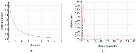
Figure 1.
The relative errors for the shape parameter approximation: K-moments. (a) the exact and approximate relationships of the shape parameter as a function of K-skewness; (b) The relative errors for the shape parameter: K-moments.
By examining this graph, one can assess the accuracy, stability, and convergence behavior of the approximation formulas across the entire range of the K-skewness coefficient. The graphical representation clearly indicates that the relative estimation errors remain below 1%, confirming the high precision and reliability of the developed expressions. Such visualization is particularly useful for identifying intervals where the approximation performs optimally and for validating the robustness of the proposed analytical relationships for practical applications in hydrological frequency analysis.
Once the shape parameter of the Weibull distribution has been determined, the remaining parameters—namely the scale and location (position) parameters—can be evaluated using the following analytical relationships. These expressions establish the link between the theoretical characteristics of the distribution and the statistical descriptors derived from the observed data, ensuring internal consistency between the estimated moments and the fitted probability model.
The scale parameter governs the dispersion and spread of the distribution, directly influencing the magnitude of the quantile values, while the location parameter defines the lower bound or shift of the distribution along the discharge axis. Together with the shape parameter, these quantities fully characterize the probabilistic behavior of the hydrological variable, allowing for accurate computation of quantiles and exceedance probabilities essential in design flood estimation.
2.2. Parameter Estimation—Method of Moments (MOM)
The expressions of the equations required for parameter estimation using the MOM are as follows:
where , and represent the arithmetic mean, the variance, and the coefficient of skewness, respectively.
However, since the skewness depends solely on the shape parameter , the latter can be approximately estimated as follows:
Figure 2 illustrates both the definition domain of the shape parameter as a function of skewness and the relative errors between the exact values and the approximate relationship used to estimate the shape parameter as a function of skewness.
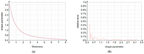
Figure 2.
The relative errors for the shape parameter approximation: MOM. (a) the exact and approximate relationships of the shape parameter as a function of skewness; (b) The relative errors for the shape parameter.
2.3. Parameter Estimation—Method of Linear Moments (L-Moments)
The exact equations for estimating the three parameters are:
In this case, the L-skewness () also depends exclusively on the shape parameter. Therefore, for this method as well, the shape parameter can be approximately estimated as a function of the L-skewness, as follows:
Figure 3 shows the variation of the shape parameter and the relative errors for the L-moments method.
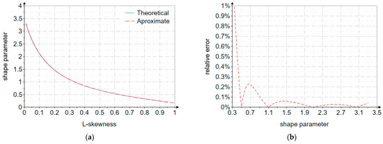
Figure 3.
The relative errors for the shape parameter approximation: L-moments. (a) the exact and approximate relationships of the shape parameter as a function of skewness; (b) The relative errors for the shape parameter.
The relationship was derived through a numerical procedure implemented in Mathcad, with the objective of obtaining an analytical expression that accurately describes the variation of with respect to , and .
The variation domain of the shape parameter was first defined based on theoretical and empirical results corresponding to the analyzed distribution. This domain was then discretized into more than 3000 equidistant values.
A graphical inspection revealed a nonlinear trend. Consequently, several types of approximation functions: polynomial, exponential, and rational, were tested and compared in terms of fitting accuracy.
The functions provided the best trade-off between analytical simplicity and numerical accuracy, yielding relative errors below 1% across the relevant range. This empirical relationship enables the direct estimation of the shape parameter thereby avoiding iterative numerical procedures commonly required in the fitting of theoretical distributions.
3. Case Study
The case studies consist of performing in situ frequency analyses of annual maximum discharges to estimate the extreme peak values associated with specific annual exceedance probabilities relevant to technical hydrology.
Considering that the method of linear moments (L-moments), the method of K-moments (K-moments), and the method of ordinary moments (MOM) rely exclusively on characteristic moments and higher-order statistical indicators to describe the probabilistic behavior of hydrological variables, their computed values for the analyzed sites are summarized in Table 1, Table 2 and Table 3.

Table 1.
Statistical indicators of the observed data derived using the MOM.
Table 2.
Statistical indicators of the observed data derived using the L-moments.
Table 3.
Statistical indicators of the observed data derived using the K-moments.
These tables provide a comparative overview of the main descriptive statistics—such as mean, coefficient of variation, skewness, and kurtosis—derived from each approach.
Where
represents the arithmetic mean;
represents the standard deviation;
represents the coefficient of variation;
represents the skewness;
represents the multiplication coefficient used in the correction of data skewness, according to common practice in Romania. This coefficient reflects the genesis of high flows, as follows: 2–for flows generated by snowmelt; 3—for flows generated by mixed sources (snowmelt and rainfall); and 4—for maximum flows generated solely by rainfall.
represents the corrected skewness.
To assess the temporal consistency of the hydrological data, a stationarity analysis was conducted using the t-test, which confirmed that the time series of annual maximum discharges did not exhibit significant trends or systematic changes over the observation period. This indicates that the dataset can be considered statistically stable and suitable for frequency analysis. Furthermore, the Grubbs test was applied to detect potential anomalous or extreme values that could distort the statistical characterization of the series; however, no outliers were identified, confirming the overall reliability and homogeneity of the observed data.
4. Results
As a case study, the performances of the Weibull distribution with the three parameters estimated with the K-moments method are presented compared to those estimated with the linear moments method.
A flood frequency analysis is performed to obtain the quantile values of annual exceedance probabilities related to rare and very rare events.
Based on the data series, the values of the extreme quantiles corresponding to the annual exceedance probabilities of 0.01%, 0.1% and 1% are determined (Table 4 and Table 5), values common in the sizing of hydrotechnical works such as dams, etc. This is also the domain of annual exceedance probabilities where the differences in estimating the quantile values are the most pronounced, representing the main inconvenience in selecting the best parameter estimation method and the best model.
Table 4.
L-moments quantile results for the Siret River.
Table 5.
L-moments quantile results for the Ialomita River.
Figure 4 presents the fitted probability distributions corresponding to the two rivers analyzed in this study. The empirical plotting positions were determined using the Hazen formula, which provides a balanced estimation of non-exceedance probabilities for observed data series. The horizontal axis is displayed on a decimal logarithmic scale, facilitating clearer visualization of the broad range of discharge values commonly associated with extreme hydrological events. This representation is particularly useful for examining the upper-tail behavior of the distributions, where rare but significant events occur and where accurate estimation is essential for hydrological design and risk assessment.
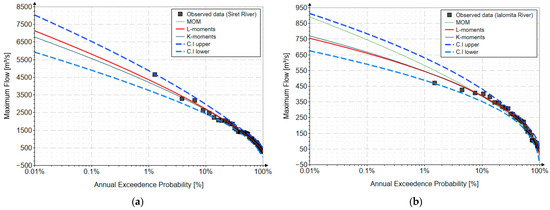
Figure 4.
The quantile function curves corresponding to the analyzed probability distribution. (a) Siret River; (b) Ialomita River.
The figure enables a comparative evaluation of the fitted distributions, highlighting how well each theoretical model replicates the empirical data. By examining both the central tendency and the tail fit, the analysis supports a better understanding of each distribution’s performance, reliability, and applicability in representing extreme river discharge behavior across different catchments.
5. Discussions
The comparative analysis between the MOM, L-moments and K-moments estimation methods highlights the capacity of the K-moments approach to provide stable and consistent parameter estimates, even in cases where data series are relatively short or include moderate variability.
For both the Siret and Ialomița Rivers, the results show that the quantiles estimated using K-moments are slightly lower than those obtained through L-moments, particularly in the upper tail of the distribution (for exceedance probabilities of 0.01–1%). This behavior suggests a more conservative estimation of extreme discharges, which may be advantageous in practical hydrological design when uncertainty in the input data is significant.
The graphical comparison of the quantile function curves (Figure 4) confirms that both methods (compared to MOM) provide a satisfactory fit to the empirical data, with the Weibull distribution adequately capturing the central tendency and variability of the observed series. However, the K-moments method demonstrates a slightly improved alignment with the empirical points in the upper-tail region, indicating its potential to better reproduce rare and extreme events.
In the case of the Siret River, the MOM method produced values that were extremely close to those obtained using the L-moments method; however, the sample (observed data) skewness was corrected in accordance with hydrological practices commonly applied in Romania. In general, the main drawback of the MOM method is that for short and medium-length series (n < 80 values), the skewness requires correction. Moreover, the hydrological practice commonly applied in Romania should be avoided, as it introduces subjectivity in selecting this correction factor, which is typically chosen arbitrarily.
The relative performance metrics—RME (Root Mean Error) and RAE (Relative Absolute Error)—reported in Table 6 further support these findings.
Table 6.
RME and RAE score values for the Siret and Ialomita Rivers.
The small differences between the L- and K-moments methods (ΔRME < 0.0003 and ΔRAE < 0.002) confirm that the proposed K-moment-based explicit relations ensure a high level of precision while maintaining computational simplicity. These results emphasize the robustness of the K-moments framework, which, unlike traditional iterative techniques, allows for explicit and reproducible parameter estimation, particularly valuable in regional or large-scale hydrological frequency studies.
The confidence interval was established using the frequency factor specific to the Weibull distribution and the K-moments method, in a manner analogous to that developed for the L- and LH-moments methods in previous studies [13], for a 95% confidence level, based on a Gaussian assumption.
The Weibull frequency factor for K-moments is:
This approach ensures internal methodological consistency, as it extends the concept of the frequency factor—traditionally employed in L-moment and LH-moment frameworks—to the K-moment method. Consequently, the estimation of quantiles and their associated uncertainty remains coherent across different moment-based approaches, enabling a direct comparison between the statistical performances of the methods.
The stability of the estimated parameters across different sites demonstrates the general applicability of the proposed relations. The similarity in coefficient of variation and skewness values obtained for both rivers reinforces the consistency of the K-moment descriptors in reflecting the statistical structure of hydrological extremes. Overall, the findings indicate that the use of explicit K-moment-based formulas can enhance both efficiency and accuracy in flood frequency analysis, reducing dependence on specialized software or iterative calibration.
6. Conclusions
This study introduces and validates explicit analytical relationships for estimating the parameters of the Weibull distribution using the K-moments method. The developed expressions provide high accuracy, with relative estimation errors below 1%, and eliminate the need for iterative numerical optimization procedures.
The main conclusions can be summarized as follows:
- K-moments offer a reliable and robust alternative to classical L-moments, ensuring numerical stability and reduced sensitivity to sampling variability.
- The proposed explicit parameter relations facilitate practical implementation of the Weibull distribution in hydrological frequency analyses, enabling fast and reproducible computations even for limited datasets.
- The comparative analysis of quantile estimates for the Siret and Ialomița rivers confirms that both methods yield similar results, with K-moments producing slightly lower and more conservative values for extreme discharges.
- Error metrics (RME and RAE) indicate negligible differences between methods, validating the high precision of the proposed approach.
- The results demonstrate that the K-moment framework can be successfully extended to other continuous probability distributions, improving accessibility and applicability in engineering hydrology and risk assessment.
The explicit relationships derived in this study contribute to simplifying and standardizing the use of the Weibull distribution for modeling hydrological extremes, providing an efficient and transparent tool for both research and practical design applications.
This research is part of broader research in which the aim is to identify the best distributions and methods for estimating their parameters for the specifics and particularities of technical hydrology in Romania [14].
Author Contributions
Conceptualization, C.G.A. and D.I.; methodology, C.G.A. and D.I.; software, C.G.A. and D.I.; validation, C.G.A. and D.I.; formal analysis, C.G.A. and D.I.; investigation, C.G.A. and D.I.; resources, C.G.A. and D.I.; data curation, C.G.A. and D.I.; writing—original draft, C.G.A. and D.I.; writing—review and editing, C.G.A. and D.I.; visualization, C.G.A. and D.I.; supervision, C.G.A. and D.I.; project administration, C.G.A. and D.I.; funding acquisition, C.G.A. and D.I. All authors have read and agreed to the published version of the manuscript.
Funding
This research received no external funding.
Data Availability Statement
The original contributions presented in this study are included in the article. Further inquiries can be directed to the corresponding author.
Conflicts of Interest
The authors declare no conflicts of interest with ACL Hydro Engineering Solutions SRL.
References
- Leščešen, I.; Šraj, M.; Basarin, B.; Pavić, D.; Mesaroš, M.; Mudelsee, M. Regional Flood Frequency Analysis of the Sava River in South-Eastern Europe. Sustainability 2022, 14, 9282. [Google Scholar] [CrossRef]
- Rima, L.; Haddad, K.; Rahman, A. Low-Flow Identification in Flood Frequency Analysis: A Case Study for Eastern Australia. Water 2024, 16, 535. [Google Scholar] [CrossRef]
- Turhan, E. An Investigation on the Effect of Outliers for Flood Frequency Analysis: The Case of the Eastern Mediterranean Basin, Turkey. Sustainability 2022, 14, 16558. [Google Scholar] [CrossRef]
- Tegegne, G.; Melesse, A.M.; Asfaw, D.H.; Worqlul, A.W. Flood Frequency Analyses over Different Basin Scales in the Blue Nile River Basin, Ethiopia. Hydrology 2020, 7, 44. [Google Scholar] [CrossRef]
- Dabire, N.; Ezin, E.C.; Firmin, A.M. Determination of Hydrological Flood Hazard Thresholds and Flood Frequency Analysis: Case Study of Nokoue Lake Watershed. Water 2025, 17, 1147. [Google Scholar] [CrossRef]
- Heo, J.-H.; Boes, D.; Salas, J. Regional Flood Frequency Analysis Based on a Weibull Model: Part 1. Estimation and Asymptotic Variances. J. Hydrol. 2001, 242, 157–170. [Google Scholar] [CrossRef]
- Chandel, N.; Agnihotri, P.G.; Patel, J.N. The Upper Narmada River Basin’s flood frequency analysis using the GAMLSS technique. Water Pract. Technol. 2025, 20, 631–652. [Google Scholar] [CrossRef]
- Gómez, Y.M.; Gallardo, D.I.; Marchant, C.; Sánchez, L.; Bourguignon, M. An In-Depth Review of the Weibull Model with a Focus on Various Parameterizations. Mathematics 2024, 12, 56. [Google Scholar] [CrossRef]
- Bardsley, E. The Weibull Distribution as an Extreme Value Model for Transformed Annual Maxima. J. Hydrol. 2019, 58, 123–131. Available online: https://www.jstor.org/stable/26912154 (accessed on 9 October 2025).
- Ekanayake, S.T.; Cruise, J.F. Comparisons of Weibull- and exponential-based partial duration stochastic flood models. Stoch. Hydrol. Hydraul. 1993, 7, 283–297. [Google Scholar] [CrossRef]
- Koutsoyiannis, D. Knowable moments for high-order stochastic characterization and modelling of hydrological processes. Hydrol. Sci. J. 2019, 64, 19–33. [Google Scholar] [CrossRef]
- Koutsoyiannis, D. Knowable Moments in Stochastics: Knowing Their Advantages. Axioms 2023, 12, 590. [Google Scholar] [CrossRef]
- Anghel, C.G. Revisiting the Use of the Gumbel Distribution: A Comprehensive Statistical Analysis Regarding Modeling Extremes and Rare Events. Mathematics 2024, 12, 2466. [Google Scholar] [CrossRef]
- Anghel, C.G.; Ianculescu, D. Application of the GEV Distribution in Flood Frequency Analysis in Romania: An In-Depth Analysis. Climate 2025, 13, 152. [Google Scholar] [CrossRef]


Disclaimer/Publisher’s Note: The statements, opinions and data contained in all publications are solely those of the individual author(s) and contributor(s) and not of MDPI and/or the editor(s). MDPI and/or the editor(s) disclaim responsibility for any injury to people or property resulting from any ideas, methods, instructions or products referred to in the content. |
© 2025 by the authors. Licensee MDPI, Basel, Switzerland. This article is an open access article distributed under the terms and conditions of the Creative Commons Attribution (CC BY) license (https://creativecommons.org/licenses/by/4.0/).