Inference for Two-Parameter Birnbaum–Saunders Distribution Based on Type-II Censored Data with Application to the Fatigue Life of Aluminum Coupon Cuts

Abstract

This study addresses the problem of parameter estimation and prediction for type-II censored data from the two-parameter Birnbaum–Saunders (BS) distribution. The BS distribution is commonly used in reliability analysis, particularly in modeling fatigue life. Accurate estimation and prediction are crucial in many fields where censored data frequently appear, such as material science, medical studies and industrial applications. This paper presents both frequentist and Bayesian approaches to estimate the shape and scale parameters of the BS distribution, along with the prediction of unobserved failure times. Random data are generated from the BS distribution under type-II censoring, where a pre-specified number of failures (m) is observed. The generated data are used to calculate the Maximum Likelihood Estimation (MLE) and Bayesian inference and evaluate their performances. The Bayesian method employs Markov Chain Monte Carlo (MCMC) sampling for point predictions and credible intervals. We apply the methods to both datasets generated under type-II censoring and real-world data on the fatigue life of 6061-T6 aluminum coupons. Although the results show that the two methods yield similar parameter estimates, the Bayesian approach offers more flexible and reliable prediction intervals. Extensive R codes are used to explain the practical application of these methods. Our findings confirm the advantages of Bayesian inference in handling censored data, especially when prior information is available for estimation. This work not only supports the theoretical understanding of the BS distribution under type-II censoring but also provides practical tools for analyzing real data in reliability and survival studies. Future research will discuss extensions of these methods to the multi-sample progressive censoring model with larger datasets and the integration of degradation models commonly encountered in industrial applications.

1. Introduction

The Birnbaum–Saunders (BS) distribution is a distribution built from the standard normal random variable using a monotone transformation method. The BS distribution is also known as the fatigue life distribution. In fact, Birnbaum and Saunders [1] introduced the distribution to model the fatigue life of metals subject to periodic stress. The BS distribution has many applications in different fields of science; fatigue failure caused under cyclic loading was provided by Birnbaum and Saunders [2] as a physical explanation of this model, and based on a biological model. Then, a more general derivation was derived by Desmond [3], who reduced some of the original propositions to strengthen the physical explanation for the use of this distribution. The hazard-rate property of the BS distribution, i.e., that it cannot be monotone and that it increases up to a point, then decreases, is the case applied to many real-life situations, as in a study of recovery from breast cancer. Langlands et al. [4] observed that the maximum mortality rate among breast cancer patients occurs about three years after the diagnosis; then, it slowly drops over a fixed interval of time.

For more details, one may refer to the comprehensive review paper by Balakrishnan and Kundu [5]. In this rich review paper, one may see other applications for the BS distribution, such as insurance data of Swedish third-party motor insurance for 1977 for one of several geographical zones, the survival life in hours for ball bearings of a certain type and the bone mineral density (BMD) measured in gm/cm² for newborn babies. In fact, the BS model has received considerable attention in the last few years for various reasons; the probability density function of a BS distribution can take on different shapes; for example, it has a non-monotonic hazard function and a nice physical justification. Furthermore, many generalizations of the BS distribution have been presented in the literature, and abundant applications in many different research areas have been found.

The cumulative distribution function (CDF) and probability density function (PDF) of the Birnbaum–Saunders model with parameters of $\alpha$ and $\beta >0$, respectively, are

$$F_T(t;\alpha ,\beta )=\mathsf{\Phi }\left[{\displaystyle \frac{1}{\alpha }}\left\{{\left({\displaystyle \frac{t}{\beta }}\right)}^{{\displaystyle \frac{1}{2}}}-{\left({\displaystyle \frac{\beta }{t}}\right)}^{{\displaystyle \frac{1}{2}}}\right\}\right],0<t<\infty ,\alpha ,\beta >0,$$

(1)

and

$$f(t;\alpha ,\beta )={\displaystyle \frac{1}{2\sqrt{2\pi }\alpha \beta }}\left[{\left({\displaystyle \frac{\beta }{t}}\right)}^{{\displaystyle \frac{1}{2}}}+{\left({\displaystyle \frac{\beta }{t}}\right)}^{{\displaystyle \frac{3}{2}}}\right]exp\left[{\displaystyle \frac{-1}{2{\alpha }^2}}\left({\displaystyle \frac{t}{\beta }}+{\displaystyle \frac{\beta }{t}}-2\right)\right],t>0,\alpha >0,\beta >0.$$

(2)

where $\alpha$ and $\beta >0$ are the shape and scale parameters, respectively, and $\mathsf{\Phi }(.)$ is the standard normal CDF. From now on, we adopt the notation of $BS$$(\alpha ,\lambda )$ to denote to the BS distribution with parameters of $\alpha$ and $\beta$. Many authors in the literature have studied different aspects of the BS distribution; among them, Birnbaum and Saunders [2] studied the maximum likelihood (ML) estimators of the shape and scale parameters of the BS model, and their asymptotic distributions were obtained by Engelhardt et al. [6]. Balakrishnan and Zhu [7] established the existence and uniqueness of the ML estimators. Ng et al. [8] discussed the ML estimation of the $\alpha$ and $\beta$ parameters based on type-II right-censored samples. Bayesian inference for the scale parameter ($\beta$) was considered by Padgett [9] with the use of a noninformative prior; it was assumed that the shape parameter was known. The same problem but when both parameters are unknown was considered by Achcar [10], and Achcar and Moala [11] addressed the problem in the case of censored data and covariates. Bayesian estimates and associated credible intervals for the parameters of the BS distribution under a general class of priors were handled by Wang et al. [12]. More recent studies further expanded the use of the BS distribution in various reliability contexts. Liu et al. [13] introduced a random-effect extension of the BS distribution to refine its modeling flexibility in reliability assessment. Sawlan et al. [14] applied the BS distribution to model metallic fatigue data, presenting its advantage in predicting fatigue life. Razmkhah et al. [15] developed a neutrosophic version of the BS distribution to account for uncertainty in data; they presented its application in industrial and environmental data analysis. Park and Wang [16] proposed a goodness-of-fit test for the BS distribution; they improved the fit evaluation of the test through a new probability plot-based approach. Finally, Dorea et al. [17] presented a generalized class of BS-type distributions that was used to model the fatigue-life data and address cases where crack damage follows heavy-tailed distributions.

Different types of censoring schemes (CSs) are adopted by authors in the literature, and the most common censoring schemes are usually called type-I and type-II CSs. Usually, the data are censored in reliability and life testing analysis. In type-II censoring, it is assumed that n items are tested. An integer of $m<n$ is pre-fixed, and as the m-th failure is observed, the experiment stops simultaneously. The prediction problem of unseen or removed observations based on the early noticed observations in the current sample has received considerable interest in numerous fields of reliability and life testing conditions. One may refer to Kaminsky and Nelson [18] for more details. The Bayesian prediction of an unseen observation from a future sample based on a current noticed sample, which is known as the informative sample, is one of the most important aspects in Bayesian analysis. Prediction can be used effectively in the medical field in predicting the future prognosis of patients or future side effects associated of patients treated with medication. For more information about the importance of the prediction problem and its different applications, one may refer to Al-Hussaini [19], Kundu and Raqab [20] and Bdair et al. [21]. The phenomenon of observing censored data is of natural interest in survival, reliability and medical studies for a wide range of reasons (see, for example, Balakrishnan and Cohen [22]). Several applications of prediction problems can be found in meteorology, hydrology, industrial stress testing, athletic events and the medical field.

Our goals in this paper are two-fold: First we employ importance sampling to compute the Bayesian estimates of $\alpha$ and $\beta$ of a BS type-II censored sample. We use very deep computer simulations to compare the executions of the Bayesian estimators with maximum likelihood estimators (MLEs). The symmetric credible intervals (CRIs) are also computed and compared to the confidence intervals (CIs) based on the asymptotic and bootstrap (Boot-t) arguments. The other goal involves considering the prediction of the life lengths of censored values. In this work, we implement the importance and Metropolis–Hastings (M–H) algorithms to estimate the posterior predictive density of unseen units based on current informative data, and we also construct the prediction intervals (PIs) of the these unseen units.

In many real-world applications, such as material testing and clinical trials, data are often incomplete due to censoring or accidental omission. Type-II censoring, in which a fixed number of failures is observed, is particularly common in reliability studies. Accurate estimation of failure parameters and predictions of unobserved data is crucial for understanding material behavior, ensuring the safety of industrial components and making informed decisions in medical research. This study presents a comprehensive comparison of frequentist and Bayesian approaches for estimating the parameters of type-II BS censored data. This paper introduces a perfect Bayesian approach that uses Markov chain Monte Carlo (MCMC) sampling to generate point estimates and credible intervals, providing a more flexible way to quantify uncertainty. The calculation of point predictions and credible intervals via this Bayesian approach effectively indicates the uncertainty associated with the predictions, providing a complete understanding of the possible range of outcomes compared to classical statistical methods. Additionally, this study applies these methods to both simulated and real-world datasets, illustrating their effectiveness in practical reliability analysis.

The practical applications of this work may cover many fields. Understanding the fatigue life of metals and other materials is important for validating the reliability of components used in auto manufacturing and structural engineering; these are some applications of materials science. The methods improved in this paper have strict ways of estimating the fatigue life of materials from censored data, which enables engineers to predict failure times accurately, which, in turn, lets them make better decisions. Another aspect of the application is medical research; it is essential to evaluate the treatment efficacy and patient prognosis, which can be achieved effectively by predicting patient survival times based on data from censored clinical trials. The Bayesian approach discussed in this work provides a useful approach to handling incomplete data and improving the accuracy of predictions. The primary objectives of this study are to explain the advantages of Bayesian inference and provide practical outlines to apply these methods in real-world reliability and survival studies.

Future research will extend the methods developed in this work to study multi-sample progressive censoring. This extension is particularly important in cases where multiple groups or samples are affected by different censoring scenarios, which usually occurs in industrial and clinical trials. By applying the methods to larger datasets, our goal will be to refine the robustness of the proposed approaches and to ensure the application of these methods to a wider range of real-world problems. Additionally, we plan to integrate degradation models, which are commonly used in industrial applications to monitor the deterioration of products over time. These models offer a deeper investigation of reliability, especially of products that deteriorate over time under stress. This approach can also provide more accurate predictions of failure times compared to classical lifetime models. With this combination of the strengths of type-II censoring, Bayesian inference and degradation modeling, we hope to offer more powerful tools for reliability and survival analysis.

The remaining sections of the paper include the following. In Section 2, we describe the determination of the MLEs of the scale and shape parameters. Asymptotic and Boot-t methods of constructing CIs of the parameters are also studied. In Section 3, we describe Bayesian estimates using importance sampling for the $\alpha$ and $\beta$ model parameters. In Section 4, Gibbs and Metropolis sampling are employed to derive sample-based estimates for the predictive density functions of the parameters, as well as the times to failure of the surviving units ($U_{s:n-m}(s=1,2,...,n-m)$) based on the noticed sample $(t_1,t_2,\dots ,t_m)$. In Section 5, we present a data analysis and a Monte Carlo simulation for numerical comparison purposes.

2. Maximum Likelihood Method

Let $T_1,\dots ,T_n$ be independent and identically distributed (iid) lifetimes with the PDF in (2) put under test. The integer of $m<n$ is pre-fixed, and the experiment stops as soon as we observe the m-th failure. The first m failure times ($t_1<\dots <t_m$) form an ordered type-II right-censored random sample, with the largest $(n-m)$ lifetimes having been censored. The likelihood function based on a type-II censored sample is given by (Balakrishnan and Cohen [22])

$$\begin{array}{ccc}\hfill L& \propto & {\left\{1-\mathsf{\Phi }\left[{\displaystyle \frac{1}{\alpha }}\xi \left({\displaystyle \frac{t_m}{\beta }}\right)\right]\right\}}^{n-m}\hfill \\ & \times & \left\{{\displaystyle \frac{1}{{\alpha }^m{\beta }^m}}\prod _{i=1}^m{\xi }^{\prime }\left({\displaystyle \frac{t_i}{\beta }}\right)\right\}exp\left[{\displaystyle \frac{-1}{2{\alpha }^2}}\sum _{i=1}^m{\xi }^2\left({\displaystyle \frac{t_i}{\beta }}\right)\right],\hfill \end{array}$$

(3)

and the log-likelihood function of (3) is

$$\begin{array}{ccc}\hfill lnL& =& \mathrm{const}+(n-m)ln\left\{1-\mathsf{\Phi }\left[{\displaystyle \frac{1}{\alpha }}\xi \left({\displaystyle \frac{t_m}{\beta }}\right)\right]\right\}-mln\alpha -mln\beta \hfill \\ & +& \sum _{i=1}^{m}ln\left[{\xi }^{\prime }\left({\displaystyle \frac{t_i}{\beta }}\right)\right]-{\displaystyle \frac{1}{2{\alpha }^2}}\sum _{i=1}^m{\xi }^2\left({\displaystyle \frac{t_i}{\beta }}\right),\hfill \end{array}$$

(4)

where

$$\xi \left(t\right)=t^{{\displaystyle \frac{1}{2}}}-t^{{\displaystyle \frac{-1}{2}}},$$

$${\xi }^2\left(t\right)=t+t^{-1}-2,$$

$${\xi }^{\prime }\left(t\right)={\displaystyle \frac{1}{2t}}\left(t^{{\displaystyle \frac{1}{2}}}+t^{{\displaystyle \frac{-1}{2}}}\right).$$

Based on Ng et al. [8], we consider

$$\begin{array}{c}\hfill {\alpha }^2={\displaystyle \frac{h_2\left(\beta \right)h_3\left(\beta \right)-h_1\left(\beta \right)h_4\left(\beta \right)}{h_1\left(\beta \right)-h_3\left(\beta \right)}}(={\phi }^2\left(\beta \right),\mathrm{say}),\end{array}$$

(5)

where

$$h_1\left(\beta \right)=\xi \left({\displaystyle \frac{t_m}{\beta }}\right),$$

$$h_2\left(\beta \right)=-{\displaystyle \frac{1}{m}}\sum _{i=1}^m{\xi }^2\left({\displaystyle \frac{t_i}{\beta }}\right),$$

$$h_3\left(\beta \right)={\left[1+\sum _{i=1}^m{\displaystyle \frac{\left(\frac{t_i}{\beta }\right){\xi }^{″}\left(\frac{t_i}{\beta }\right)}{{\xi }^{\prime }\left(\frac{t_i}{\beta }\right)}}\right]}^{-1}\left({\displaystyle \frac{t_m}{\beta }}\right){\xi }^{\prime }\left({\displaystyle \frac{t_m}{\beta }}\right),$$

$$h_4\left(\beta \right)={\left[1+\sum _{i=1}^m{\displaystyle \frac{\left(\frac{t_i}{\beta }\right){\xi }^{″}\left(\frac{t_i}{\beta }\right)}{{\xi }^{\prime }\left(\frac{t_i}{\beta }\right)}}\right]}^{-1}\left[-{\displaystyle \frac{1}{m}}\sum _{i=1}^m\left({\displaystyle \frac{t_i}{\beta }}\right)\xi \left({\displaystyle \frac{t_i}{\beta }}\right){\xi }^{\prime }\left({\displaystyle \frac{t_i}{\beta }}\right)\right].$$

Then, we consider

$$\begin{array}{ccc}\hfill Q\left(\beta \right)& =& {\phi }^2\left(\beta \right)\left[{\displaystyle \frac{1}{2}}-{\displaystyle \frac{1}{K^{\ast }\left(\beta \right)}}\right]-{\displaystyle \frac{u^{\ast }}{2}}+{\displaystyle \frac{1}{2v^{\ast }}}\hfill \\ & -& {\displaystyle \frac{\phi \left(\beta \right)(n-m)}{m}}H\left[{\displaystyle \frac{1}{\phi \left(\beta \right)}}\xi \left({\displaystyle \frac{t_m}{\beta }}\right)\right]\left({\displaystyle \frac{t_m}{\beta }}\right){\xi }^{\prime }\left({\displaystyle \frac{t_m}{\beta }}\right),\hfill \end{array}$$

where

$$u^{\ast }={\displaystyle \frac{1}{m}}\sum _{i=1}^m\left({\displaystyle \frac{t_i}{\beta }}\right),$$

$$v^{\ast }={\left[{\displaystyle \frac{1}{m}}\sum _{i=1}^m{\left({\displaystyle \frac{t_i}{\beta }}\right)}^{-1}\right]}^{-1},$$

$$K^{\ast }\left(\beta \right)={\left[{\displaystyle \frac{1}{m}}\sum _{i=1}^m{\left(1+{\displaystyle \frac{t_i}{\beta }}\right)}^{-1}\right]}^{-1},$$

and

$$K^{\prime \ast }\left(\beta \right)={\left[K^{\ast }\left(\beta \right)\right]}^2\left[{\displaystyle \frac{1}{m}}\sum _{i=1}^m{\left(1+{\displaystyle \frac{t_i}{\beta }}\right)}^{-2}\right].$$

The ML estimate of $\beta$ is the solution of $Q\left(\beta \right)=0$. The nonlinearity of $Q\left(\beta \right)=0$ urges us to use a numerical procedure to solve it for $\beta$. The positive square root of the right-hand side of (5) gives the maximum likelihood estimate ($\widehat{\alpha }$ of $\alpha$) after calculating the ML estimate ($\widehat{\beta }$) of $\beta$.

To construct confidence intervals for $\alpha$ and $\beta$, we need the observed Fisher information matrix $\left(\mathbb{J}\left({\widehat{\delta }}_M\right)\right)$, which is the negative of second partial derivatives of the log-likelihood function in (4). It is well-known that the approximation of ${\widehat{\delta }}_M\sim N_2(\delta ,{\mathbb{J}}^{-1}\left({\widehat{\delta }}_M\right))$ is applicable, where $\delta =(\alpha ,\beta )$ and ${\widehat{\delta }}_M=({\widehat{\alpha }}_M,{\widehat{\beta }}_M)$. Therefore, the approximations of $100(1-\gamma )\%$ CIs for $\alpha$ and $\beta$ are $\left({\widehat{\alpha }}_M-z_{\gamma /2}\sqrt{{\upsilon }_{11}},{\widehat{\alpha }}_M+z_{1-\gamma /2}\sqrt{{\upsilon }_{11}}\right)$ and $\left({\widehat{\beta }}_M-z_{\gamma /2}\sqrt{{\upsilon }_{22}},{\widehat{\beta }}_M+z_{1-\gamma /2}\sqrt{{\upsilon }_{22}}\right)$, respectively, where ${\upsilon }_{11}$ and ${\upsilon }_{22}$ are the elements of the main diagonal of ${\mathbb{J}}^{-1}\left({\widehat{\delta }}_M\right)$ and $z_{\gamma }$ is $100\gamma$-th upper-point percentile of the standard Gaussian distribution. Usually, for small sample sizes, the CI based on the asymptotic result does not perform well in calculating the CI. For this reason, the CI based on the Boot-t method is an effective method in evaluating the CI; one may refer to, for example, Ahmed [23]. The algorithm that best describes this method is summarized as follows:

• Step 1: Use the ML estimation to estimate $\alpha$ and $\beta$ based on the observed informative sample (denoted by ${\widehat{\alpha }}_M$ and ${\widehat{\beta }}_M)$;
• Step 2: Generate a Boot-t sample using ${\widehat{\alpha }}_M$ and ${\widehat{\beta }}_M$ obtained in Step 1; then, calculate the first m observed censored units ($B_{U\left(1\right)},B_{U\left(2\right)},\dots ,B_{U\left(m\right)}$) under the BS model. Next, compute the corresponding MLEs (${\widehat{\alpha }}_M^{\ast }$ and ${\widehat{\beta }}_M^{\ast }$) of $\alpha$ and $\beta$ and the elements $({\upsilon }_{11}^{\ast },{\upsilon }_{22}^{\ast })$ of the main diagonal of $J^{{\ast }^{-1}}({\widehat{\alpha }}_M^{\ast },{\widehat{\beta }}_M^{\ast })$;
• Step 3: Define an estimated Boot-t version,

  $$Q_1^{\ast }={\displaystyle \frac{{\widehat{\alpha }}_M^{\ast }-{\widehat{\alpha }}_M}{\sqrt{{\upsilon }_{11}^{\ast }}}},\mathrm{and}{Q}_2^{\ast }={\displaystyle \frac{{\widehat{\beta }}_M^{\ast }-{\widehat{\beta }}_M}{\sqrt{{\upsilon }_{22}^{\ast }}}},$$

  depending on the Boot-t sample generated in Step 2;
• Step 4: Generate M = 1000 Boot-t samples and versions of $Q_1^{\ast }$ and $Q_2^{\ast }$; then, obtain the $100(\gamma /2)$-th and $100(1-\gamma /2)$-th sample quantiles of $Q_1^{\ast }$ and $Q_2^{\ast }$;
• Step 5: Compute the approximate $100(1-\gamma )\%$ CIs for $\alpha$ and $\beta$ as
  $({\widehat{\alpha }}_M-{\widehat{q}}_{1,1-\gamma /2}\sqrt{{\upsilon }_{11}},{\widehat{\alpha }}_{ML}-{\widehat{q}}_{1,\gamma /2}\sqrt{{\upsilon }_{11}})$ and $({\widehat{\beta }}_{ML}-{\widehat{q}}_{2,1-\gamma /2}\sqrt{{\upsilon }_{22}},{\widehat{\beta }}_{ML}-{\widehat{q}}_{2,\gamma /2}\sqrt{{\upsilon }_{22}})$.

3. Bayesian Method

Here, based on a type-II censored sample from the two-parameter BS distribution, we obtain the posterior densities of the $\alpha$ and $\beta$ parameters in order to present the corresponding Bayesian estimators of the mentioned parameters. To develop the Bayesian estimates, we first present independent priors for $\alpha$ and $\beta$ based on the approximation presented by Tsay et al. [24]. Tsay et al. [24] stated that the error function ($erf(.)$) can be written in a form of exponential function as

$$erf\left(z\right)=1-exp\{-c_{1}z-c_2{z}^2\},$$

(6)

where $c_1=1.0950$ and $c_2=0.7565$. It is well known that the standard normal CDF can be written in terms of $erf(.)$ as

$$\begin{array}{ccc}\hfill \mathsf{\Phi }\left(x\right)& =& {\displaystyle \frac{1}{\sqrt{2\pi }}}{\int }_{-\infty }^x{e}^{{\displaystyle \frac{-t^2}{2}}dt}\hfill \\ & =& {\displaystyle \frac{1}{2}}\left[1+erf\left({\displaystyle \frac{x}{\sqrt{2}}}\right)\right].\hfill \end{array}$$

(7)

Using (6) and (7), we conclude that

$$\begin{array}{ccc}\hfill 1-\mathsf{\Phi }\left[{\displaystyle \frac{1}{\alpha }}\xi \left({\displaystyle \frac{t_i}{\beta }}\right)\right]& \approx & {\displaystyle \frac{1}{2}}exp\left\{-c_1\left({\displaystyle \frac{1}{\sqrt{2}\alpha }}\xi \left({\displaystyle \frac{t_i}{\beta }}\right)\right)-c_2{\left({\displaystyle \frac{1}{\sqrt{2}\alpha }}\xi \left({\displaystyle \frac{t_i}{\beta }}\right)\right)}^2\right\}\hfill \\ & =& {\displaystyle \frac{1}{2}}exp\left\{{\displaystyle \frac{-c_1}{\sqrt{2}\alpha }}\xi \left({\displaystyle \frac{t_i}{\beta }}\right)\right\}exp\left\{{\displaystyle \frac{-c_2}{2{\alpha }^2}}{\xi }^2\left({\displaystyle \frac{t_i}{\beta }}\right)\right\}.\hfill \end{array}$$

(8)

According to (8), the likelihood function in (3) can be approximated by

$$\begin{array}{ccc}\hfill L& \propto & \left\{{\displaystyle \frac{1}{{\alpha }^m{\beta }^m}}\prod _{i=1}^m{\xi }^{\prime }\left({\displaystyle \frac{t_i}{\beta }}\right)\right\}exp\left[{\displaystyle \frac{-1}{2{\alpha }^2}}\sum _{i=1}^m{\xi }^2\left({\displaystyle \frac{t_i}{\beta }}\right)\right]\hfill \\ & \times & exp\left\{{\displaystyle \frac{-c_1(n-m)}{\sqrt{2}\alpha }}\xi \left({\displaystyle \frac{t_m}{\beta }}\right)\right\}exp\left\{{\displaystyle \frac{-c_2(n-m)}{2{\alpha }^2}}{\xi }^2\left({\displaystyle \frac{t_m}{\beta }}\right)\right\}\hfill \\ & \propto & {\displaystyle \frac{1}{{\alpha }^m{\beta }^m}}\prod _{i=1}^m{\xi }^{\prime }\left({\displaystyle \frac{t_i}{\beta }}\right)exp\left\{{\displaystyle \frac{-1}{2{\alpha }^2}}\left[\sum _{i=1}^m{\xi }^2\left({\displaystyle \frac{t_i}{\beta }}\right)+c_2(n-m){\xi }^2\left({\displaystyle \frac{t_m}{\beta }}\right)\right]\right\}\hfill \\ & \times & exp\left\{{\displaystyle \frac{-c_1(n-m)}{\sqrt{2}\alpha }}\xi \left({\displaystyle \frac{t_m}{\beta }}\right)\right\}.\hfill \end{array}$$

(9)

If we use non-informative priors, improper posterior and continuous conjugate priors result, so we use the proper priors with known hyperparameters to support the property of posteriors. As stated by Wang et al. [12], we assume that $\beta$ has an inverse gamma $\left(IG\right)$ distribution, with parameters $(a_1,b_1)$ denoted by $IG\left(\beta \right|a_1,b_1)$, and that $\lambda =2{\alpha }^2$ also has an inverse gamma distribution with parameters $(a_2,b_2)$ denoted by $IG\left(\lambda \right|a_2,b_2)$ with the following densities:

$${\nu }_{\beta }\left(a_1,b_1\right)={\displaystyle \frac{b_1^{a_1}}{\mathsf{\Gamma }\left(a_1\right)}}{\beta }^{-a_1-1}{e}^{{\displaystyle \frac{-b_1}{\beta }}},{\nu }_{\lambda }\left(a_2,b_2\right)={\displaystyle \frac{b_2^{a_2}}{\mathsf{\Gamma }\left(a_2\right)}}{\lambda }^{-a_2-1}{e}^{{\displaystyle \frac{-b_2}{\lambda }}},$$

(10)

where $a_1,b_1,a_2,b_2$ are positive real constants that mirror prior knowledge about the $\beta$ and $\lambda$ parameters. By combining (9) and (10), the joint posterior density of $\beta$ and $\lambda$ can be written as

$$\begin{array}{ccc}\hfill p(\lambda ,\beta |T)& \propto & L(\lambda ,\beta ;T)\pi \left(\beta \right|a_1,b_1)\pi \left(\lambda \right|a_2,b_2)\hfill \\ & \propto & {\nu }_{\beta }(a_1+m,b_1){\nu }_{\lambda }\left(a_2+{\displaystyle \frac{m}{2}},\sum _{i=1}^m{\xi }^2\left({\displaystyle \frac{t_i}{\beta }}\right)+c_2(n-m){\xi }^2\left({\displaystyle \frac{t_m}{\beta }}\right)+b_2\right)\hfill \\ & \times & {\delta }_m\left(\beta \right){\tau }_m(\lambda ,\beta ){\left(\sum _{i=1}^m{\xi }^2\left({\displaystyle \frac{t_i}{\beta }}\right)+c_2(n-m){\xi }^2\left({\displaystyle \frac{t_m}{\beta }}\right)+b_2\right)}^{-(a_2+{\displaystyle \frac{m}{2}})},\hfill \end{array}$$

where

$${\delta }_m\left(\beta \right)=\prod _{i=1}^m{\xi }^{\prime }\left({\displaystyle \frac{t_i}{\beta }}\right),$$

and

$${\tau }_m(\lambda ,\beta )=exp\left\{{\displaystyle \frac{-c_1(n-m)}{\sqrt{\lambda }}}\xi \left({\displaystyle \frac{t_m}{\beta }}\right)\right\}.$$

Based on the observed type-II censored sample, the marginal density of $\beta$ is given by

$$\begin{array}{c}\hfill \pi \left(\beta \right|\mathbb{T})\propto {\nu }_{\beta }(a_1+m,b_1)\omega \left(\beta \right),\end{array}$$

where

$$\omega \left(\beta \right)={\left(\sum _{i=1}^m{\xi }^2\left({\displaystyle \frac{t_i}{\beta }}\right)+c_2(n-m){\xi }^2\left({\displaystyle \frac{t_m}{\beta }}\right)+b_2\right)}^{-(a_2+{\displaystyle \frac{m}{2}})}{\delta }_m\left(\beta \right)E_{\lambda }\left({\tau }_m(\lambda ,\beta )\right),$$

with $E_{\lambda }$ denoting the expectation with respect to $IG(a_2+{\displaystyle \frac{m}{2}},{\sum }_{i=1}^m{\xi }^2\left({\displaystyle \frac{t_i}{\beta }}\right)+c_2(n-m){\xi }^2\left({\displaystyle \frac{t_m}{\beta }}\right)+b_2)$. The conditional density of $\lambda$, given $\beta$ and the data, is

$$\begin{array}{c}\hfill \nu \left(\lambda \right|\beta ,\mathbb{T})\propto {\nu }_{\lambda }\left(a_2+{\displaystyle \frac{m}{2}},\sum _{i=1}^m{\xi }^2\left({\displaystyle \frac{t_i}{\beta }}\right)+c_2(n-m){\xi }^2\left({\displaystyle \frac{t_m}{\beta }}\right)+b_2\right){\tau }_m(\lambda ,\beta ).\end{array}$$

(11)

Now, we proceed to obtain the Bayesian estimators (BEs) of $\alpha$ and $\beta$ under the squared error loss (SEL) function. The BE of any function of $\alpha$ and $\beta$ (e.g., $\theta =\eta (\alpha ,\beta )$) under the SEL function is given by

$$\begin{array}{c}\hfill {\widehat{\theta }}_{SE}={\displaystyle \frac{{\int }_0^{\infty }{\int }_0^{\infty }\eta (\alpha ,\beta )g_1\left(\alpha \right|\mathbf{x},\beta )g_2\left(\beta \right|\mathbf{x})h\left(\beta \right|\mathbf{x})}{{\int }_0^{\infty }{\int }_0^{\infty }{g}_1\left(\alpha \right|\mathbf{x},\beta )g_2\left(\beta \right|\mathbf{x})h\left(\beta \right|\mathbf{x})}}.\end{array}$$

(12)

The BEs for $\alpha$ and $\beta$ cannot be obtained in explicit form because (12) cannot be evaluated analytically. For this reason, we use an importance sampling technique, as suggested by Chen and Shao [25], to approximate (12) and to construct the corresponding credible intervals. Based on the observed type-II censored sample, the Bayes estimator of $\beta$ is written as

$${\widehat{\beta }}_B=E\left(\beta \right|\mathbb{T})={\displaystyle \frac{E_{\beta }\left(\beta \omega \left(\beta \right)\right)}{E_{\beta }\left(\omega \left(\beta \right)\right)}},$$

(13)

where $E_{\beta }$ denotes the expectation with respect to $IG(a_1+m,b_1)$. Based on (11), we also have

$$E\left(\lambda |\beta ,\mathbb{T}\right)={\displaystyle \frac{E_{\lambda }\left[\lambda {\tau }_m(\lambda ,\beta )\right]}{E_{\lambda }\left[{\tau }_m(\lambda ,\beta )\right]}}.$$

As a result, the Bayesian estimate of $\lambda$ can be written as

$$\begin{array}{ccc}\hfill {\widehat{\lambda }}_B=E\left(\lambda |T\right)& =& E_{\beta }{E}_{\lambda }\left(\lambda |\beta ,T\right)\hfill \\ & =& {\displaystyle \frac{E_{\beta }\left(\omega \left(\beta \right)E\left(\lambda |\beta ,\mathbb{T}\right)\right)}{E_{\beta }\left(\omega \left(\beta \right)\right)}}.\hfill \end{array}$$

(14)

Equations (13) and (14) cannot be solved analytically, so to produce consistent sample-based estimators for $\lambda$ and $\beta$ and to construct corresponding credible intervals, we employ an importance sampling technique to approximate Equations (13) and (14). The Bayesian point estimators of $\lambda$ and $\beta$ can be determined using the following algorithm:

• Importance sampling algorithm

1.

Generate M values of $\beta$ from $IG(a_1+m,b_1)$ (say, ${\beta }_i,i=1,2,\dots ,M$);

2.

For each ${\beta }_i$ generated in Step 1, generate M values of $\lambda$ from

$IG\left(a_2+{\displaystyle \frac{m}{2}},{\sum }_{i=1}^m{\xi }^2\left({\displaystyle \frac{t_i}{\beta }}\right)+c_2(n-m){\xi }^2\left({\displaystyle \frac{t_m}{\beta }}\right)+b_2\right)$;

3.

Compute $E_{\lambda }\left[\lambda {\tau }_m(\lambda ,\beta )\right]$ and $E_{\lambda }\left[{\tau }_m(\lambda ,\beta )\right]$ with respect to the $\lambda$ values simulated in Step 2;

4.

Compute $\omega \left({\beta }_i\right)$ and $E\left(\lambda \right|{\beta }_i,\mathbb{T})$;

5.

Average the numerators and the denominators of (13) and (14) with respect to the $\beta$ values simulated in Step 1.

Now, the two-sided Bayesian credible confidence intervals, as well as the highest posterior density (HPD) CIs for $\alpha$ and $\beta$, can be improved here. Using the simulated values, $100(1-\gamma )\%$ Bayesian CIs for the $\alpha$ and $\beta$ parameters can be computed. Therefore, a $100(1-\gamma )\%$ Bayesian CI for $\theta (\theta =\alpha$, or $\beta$) is $\left({\theta }_{[100\gamma /2]},{\theta }_{\left[100\right(1-\gamma /2\left)\right]}\right)$, where ${\theta }_{\left[100\gamma \right]}$ is the $100\gamma$-th percentile of the $\theta$ values simulated using the above algorithm, with $\left[x\right]$ being the integer part of x. Since the Bayesian credible CIs do not clarify whether the values of $\theta$ located inside these intervals have a higher probability than the values located outside the intervals, we present the HPD CI for $\theta$. The HPD CI is considered one of the shortest-width CIs; here, the posterior density of any point outside the interval is less than that of any point within the interval. We use a Monte Carlo technique for importance sampling, which was first presented by Chen and Shao [25] to address the HPD CI for any function of the involved parameters (e.g., $\varrho (\alpha ,\beta )$). We start by arranging the simulated values of $\varrho (\alpha ,\beta )$ in ascending order to get

$${\varrho }_{\left(1\right)}\le {\varrho }_{\left(2\right)}\le \dots \le {\varrho }_{\left(M\right)},$$

then compute the ratios as

$${\zeta }_i={\displaystyle \frac{\omega \left({\beta }_{\left(i\right)}\right)}{{\sum }_{i=1}^M\omega \left({\beta }_{\left(i\right)}\right)}},i=1,2,\dots ,M.$$

Taking in consideration the fact that M is sufficiently large, the $100(1-\gamma )\%$ HPD interval for $\varrho$ is the shortest interval among the intervals ($I_j$) for $j=1,2,\dots ,M-\left[\right(1-\gamma \left)M\right]$, with

$$I_j=\left({\varrho }^{({\displaystyle \frac{j}{M}})},{\varrho }^{({\displaystyle \frac{j+\left[\right(1-\gamma \left)M\right]}{M}})}\right),$$

where ${\varrho }^{\left(\gamma \right)}$ is $100\gamma$-th percentile of $\varrho$, which can be taken out as follows:

$$\begin{array}{ccc}\hfill {\varrho }^{\left(\gamma \right)}& =& \left\{\begin{array}{cc}{\varrho }_{\left(1\right)}\hfill & if\gamma =0,\hfill \\ & \\ {\varrho }_{\left(i\right)}\hfill & if\sum _{j=1}^{i-1}{\zeta }_j\le \gamma \le \sum _{j=1}^i{\zeta }_j,\hfill \end{array}\right.\hfill \end{array}$$

Then, the HPD CIs of $\alpha$ and $\beta$ can be obtained accordingly.

4. Bayesian Prediction Method

Here, we discuss the problem of predicting the unseen items in the type-II censored data from the BS distribution. Precisely, our main interest is in the posterior density of the s-th-order statistic from a sample of size $n-m$ unseen items. For this, we predict $U_{s:n-m}(s=1,2,\dots ,n-m)$ based on the observed type-II censored sample $(t_1,t_2,...,t_m)$. We start by presenting the posterior predictive density of $Y=U_{s:n-m}$, given the observed censored data, which has the form of

$$\begin{array}{ccc}\hfill p\left(y\right|\mathrm{data})& =& {\int }_0^{\infty }{\int }_0^{\infty }{f}_{Y|\mathrm{data}}\left(y\right|\alpha ,\beta )\pi (\alpha ,\beta |\mathrm{data})d\alpha d\beta ,y>t_m,\hfill \end{array}$$

(15)

where $f_{Y|\mathrm{data}}\left(y\right|\alpha ,\beta )$ is the conditional density function of Y, given T = t. According to the Markovian property of order statistics (Arnold et al. [26]), this conditional density is just the conditional density of Y given $t_m$, that is, the pdf of the s-th-order statistic out of a sample of $n-m$ from F left truncated at $t_m$. Precisely, it can be rewritten as $f_{Y|\mathrm{data}}\left(y\right|\alpha ,\beta )=f_{Y|T=t_m}\left(y\right|\alpha ,\beta )$.

Let us consider the case when $s=m+1$, in which case

$$\begin{array}{ccc}\hfill f_{t_{m+1}|t_m}\left(y\right|\alpha ,\beta )& =& {\displaystyle \frac{(n-m)f(y;\alpha ,\beta ){\left(1-F(y;\alpha ,\beta )\right)}^{n-m-1}}{{\left(1-F(t_m;\alpha ,\beta )\right)}^{n-m}}},y>t_m\hfill \\ & =& {\displaystyle \frac{\frac{(n-m)}{2\sqrt{2\pi \alpha \beta }}\left[{\left(\frac{\beta }{y}\right)}^{\frac{1}{2}}-{\left(\frac{y}{\beta }\right)}^{\frac{3}{2}}\right]exp\left[\frac{-\left(\frac{y}{\beta }+\frac{\beta }{y}-2\right)}{2{\alpha }^2}\right]{\left(1-\mathsf{\Phi }\left[\frac{1}{{\alpha }_j}\xi \left(\frac{y}{{\beta }_j}\right)\right]\right)}^{n-m-1}}{{\left(1-\mathsf{\Phi }\left[\frac{1}{{\alpha }_j}\xi \left(\frac{t_m}{{\beta }_j}\right)\right]\right)}^{n-m}}}.\hfill \end{array}$$

(16)

The predictive density of $t_{m+1}$ at any point ($y>t_m$) is then

$$\begin{array}{ccc}\hfill f_{t_{m+1}|t_m}^{\ast }\left(y\right|\mathrm{data})& =& {\int }_0^{\infty }{\int }_0^{\infty }{f}_{t_{m+1}|t_m}\left(y\right|\alpha ,\beta )\pi (\alpha ,\beta |\mathrm{data})d\alpha d\beta ,y>t_m.\hfill \end{array}$$

(17)

Visibly, the Bayesian predictive estimate ($E\left(Y\right|\mathrm{data})$) cannot be evaluated directly from (15) and (17). Therefore, we suggest Monte Carlo (MC) simulation to create a sample from the predictive distribution. Under the squared error loss (SEL) function, the Bayesian predictors (BPs) of $Y=t_s$ can be computed as

$$\widehat{Y}=E_{posterior}\left(Y\right|\mathrm{data})={\int }_{t_m}^{\infty }yp\left(y\right|\mathrm{data})dy.$$

Based on MC samples $\left\{\left({\alpha }_j,{\beta }_j\right):j=1,\dots ,M\right\}$, the simulation-based estimator of $p\left(y\right|x)$ can be computed as

$$\widehat{p}\left(y\right|\mathrm{data})={\displaystyle \frac{1}{M}}\sum _{j=1}^{M}f\left(y|t_m;{\alpha }_j,{\beta }_j\right).$$

(18)

Using algebra, the sample-based predictor of Y can be simplified as follows:

$$\begin{array}{ccc}\hfill \widehat{Y}& =& {\displaystyle \frac{1}{M}}\sum _{j=1}^M\sum _{i=0}^{s-1}\sum _{l=0}^{n-m-s}{(-1)}^{i+l}\left({\displaystyle \genfrac{}{}{0pt}{}{s-1}{i}}\right)\left({\displaystyle \genfrac{}{}{0pt}{}{n-m-s}{l}}\right){\displaystyle \frac{{\beta }_j}{2}}{\displaystyle \frac{{\mathsf{\Phi }}^i\left[\frac{1}{{\alpha }_j}\xi \left(\frac{t_m}{{\beta }_j}\right)\right]}{{\left(1-\mathsf{\Phi }\left[\frac{1}{{\alpha }_j}\xi \left(\frac{t_m}{{\beta }_j}\right)\right]\right)}^{n-m}}}\hfill \\ & \times & {\int }_{{\displaystyle \frac{1}{{\alpha }_j}}\xi \left({\displaystyle \frac{t_m}{{\beta }_j}}\right)}^{\infty }{\left[{\alpha }_{j}u+\sqrt{{\left({\alpha }_{j}u\right)}^2+4}\right]}^2{\left[\mathsf{\Phi }\left(u\right)\right]}^{s+l-1-i}{e}^{-{\displaystyle \frac{u^2}{2}}}du.\hfill \end{array}$$

Furthermore, the approximate estimator given in (18) can be used to find a two-sided prediction interval for Y. The $100(1-\gamma )\%$ prediction interval for Y is $(L,U)$, where L and U can be computed numerically as

$$P\left(Y>L|t\right)={\int }_L^{\infty }\widehat{p}\left(y\right|t)dy=1-{\displaystyle \frac{\gamma }{2}}, \mathrm{and}P\left(Y>U|t\right)={\int }_U^{\infty }\widehat{p}\left(y\right|t)dy={\displaystyle \frac{\gamma }{2}}.$$

Now, we discuss the use of the Gibbs sampler in estimating the posterior distribution. In fact, to estimate the posterior distribution using the Gibbs sampler, we need to generate samples from the full conditional distribution for each quantity involved. This is true for $\alpha$ and $Y=(t_{m+1},t_{m+2},\cdots ,t_n)$ but not for $\beta$. Consequently, we adopt the M–H algorithm in combination with the Gibbs sampler to sample $\alpha$ and Y directly from their full conditional distributions. We update $\beta$ via an M–H algorithm, as explained by Tierney [27], i.e., the normal distribution is the proposal distribution. Using the extended likelihood in (9) and the joint prior of $\beta$ and $\lambda$, the full Bayesian model can be written as

$$\pi (\lambda ,\beta |\mathbb{T})\propto {\varphi }_1\left(\lambda \right|\beta ,\mathbb{T}){\varphi }_2\left(\beta \right|\mathbb{T}),$$

where ${\varphi }_1\left(\lambda \right|\beta ,\mathbb{T})$ is the PDF of the inverse gamma distribution ($IG\left(a_2+{\displaystyle \frac{m}{2}},{\sum }_{i=1}^m{\xi }^2\left({\displaystyle \frac{t_i}{\beta }}\right)+c_2(n-m){\xi }^2\left({\displaystyle \frac{t_m}{\beta }}\right)+b_2\right)$) and ${\varphi }_2\left(\beta \right|\mathbb{T})$ is given by

$$\begin{array}{ccc}\hfill {\varphi }_2\left(\beta \right|\mathbb{T})& \propto & {\nu }_{\beta }(a_1+m,b_1){\delta }_m\left(\beta \right){\tau }_m(\lambda ,\beta )\hfill \\ & \times & {\left(\sum _{i=1}^m{\xi }^2\left({\displaystyle \frac{t_i}{\beta }}\right)+c_2(n-m){\xi }^2\left({\displaystyle \frac{t_m}{\beta }}\right)+b_2\right)}^{-(a_2+{\displaystyle \frac{m}{2}})}.\hfill \end{array}$$

(19)

It can be easily seen that the full conditional distribution of $\lambda$, given $\beta$ and $\mathbb{T}$, is a known distribution, while the form of the full conditional distribution of $\beta$, given $\mathbb{T}$, in (19) is not a well-known distribution; therefore, we cannot generate $\beta$ directly. Accordingly, to generate $\beta$ from the full conditional distribution of $\beta$, given $\mathbb{T}$, we use the M–H algorithm with normal proposed distribution. One of the important things in this process is to decrease the rejection rate among all iterations as much as possible. Below, we present an algorithm that depends on the choice of the normal distribution as a proposal distribution and on the use of the M–H algorithm. This method can also be used to find the BEs and to structure the credible intervals for $\lambda$ and $\beta$. The Gibbs sampler is considered a Markov chain Monte Carlo (MCMC) technique that simulates a Markov chain based on the full conditional distributions. We use the Gibbs sampler to obtain an approximation of ${\theta }_{BE}$ and the corresponding credible intervals based on the drawing of MCMC samples ($({\lambda }_l,{\beta }_l),l=1,2,...,M$) from the joint posterior distribution. For this reason, we present the M–H algorithm according to the following steps:

• M–H algorithm for prediction

1.

Start with the MLEs $(\widehat{\alpha },\widehat{\beta })$ as the initial values (e.g., $({\alpha }^{\left(0\right)},{\beta }^{\left(0\right)})$);

2.

Set J = 1;

3.

Given ${\beta }^{(J-1)}$, generate $\beta$ from ${\varphi }_2\left(\beta \right|\mathbb{T})$ in (19) with $N({\beta }^{(J-1)},S_{\beta }^2)$ as the proposal distribution, where $S_{\beta }^2$ is the variance of $\beta$, which can be picked out to be the inverse of the Fisher information. The new values of $\beta$ can be updated as follows:

a.

Generate ${\zeta }_J$ from $N({\beta }^{(J-1)},S_{\beta }^2)$ and u from $U(0,1)$;

b.

If $u<min(1,\epsilon )$, then let ${\beta }^{\left(J\right)}={\zeta }_J$; otherwise, go to (a), where

$$\epsilon ={\displaystyle \frac{\pi \left({\zeta }_J\right|\mathbf{T})}{\pi \left({\beta }^{(J-1)}\right|\mathbf{T})}};$$

4.

Given $\beta$, generate $\alpha =\sqrt{{\displaystyle \frac{\lambda }{2}}}$ from $IG\left(a_2+{\displaystyle \frac{m}{2}},{\sum }_{i=1}^m{\xi }^2\left({\displaystyle \frac{t_i}{\beta }}\right)+c_2(n-m){\xi }^2\left({\displaystyle \frac{t_m}{\beta }}\right)+b_2\right)$;

5.

Set $J=J+1$;

6.

Repeat Steps 3–5 M times;

5. Data Analysis and Simulation

Here, an inclusive simulation study is performed to assess the performance of the sample-based estimates and predictors presented in the previous few sections, and we discuss the analysis of data extracted from a type-II censored BS model. All calculations are carried out using R programming software. The Pseudocodes for the Bayesian Estimation and Prediction, Core Functions in R and Software Versions are presented in the Appendix A, Appendix B, Appendix C and Appendix D, respectively.

5.1. Real Data Analysis

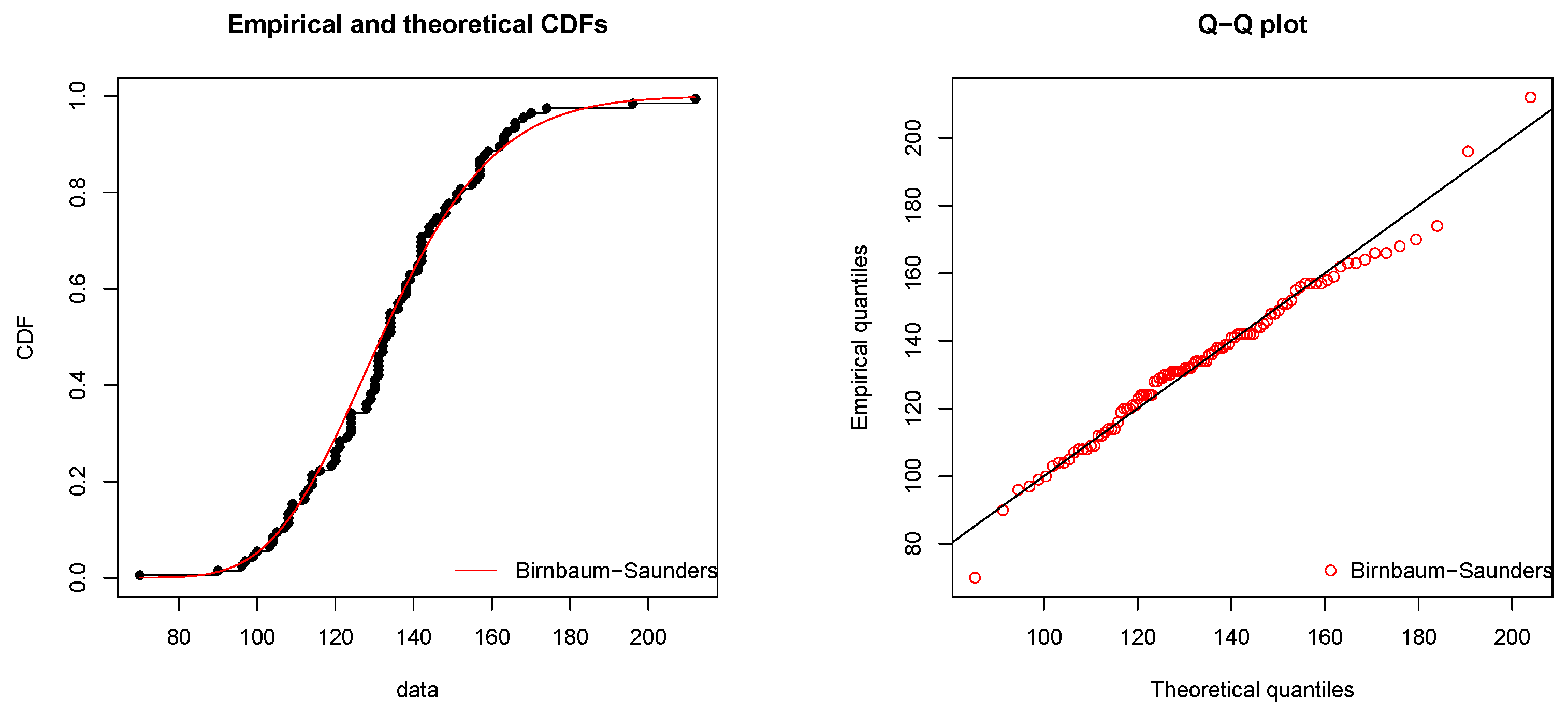
In this subsection, we start by presenting the analysis of a real dataset to explain the execution of the previously presented methods. The data represent the fatigue life of 6061-T6 aluminum coupons cut parallel to the direction of rolling and oscillated at 18 cycles per second with a maximum stress per cycle of 31,000 psi. These data were originally reported by Birnbaum and Saunders [2]. The dataset is expressed as follows:

70     90    96     97    99    100      103      104  104  105  107  108  108  108  109

109  112  112  113  114  114  114  116  119  120  120  120  121  121  123

124  124  124  124  124  128  128  129  129  130  130  130  131  131  131

131  131  132  132  132  133  134  134  134  134  134  136  136  137  138

138  138  139  139  141  141  142  142  142  142  142  142  144  144  145

146  148  148  149  151  151  152  155  156  157  157  157  157  158  159

162  163  163  164  166  166  168  170  174  196  212

For illustrative purposes, we suggest the following type-II censored samples with ($n=101$, $m=90$) and ($n=101$, $m=70$), i.e., we suggest only 90 and 70 available observations. Before we proceed with further analysis, we first present some basic descriptive statistics concluded from this dataset. The mean, the standard deviation and the coefficient of skewness are 133.73, 22.36 and 0.3355, respectively. The BS model may be used to analyze this dataset because the data are positively skewed. Now, we can simply numerically check the fit of the dataset. The Newton—Raphson method is employed to evaluate the MLEs of the parameters of the BS model. The MLEs of the shape and scale parameters are $\widehat{\alpha }$ = 0.1704 and $\widehat{\beta }$ = 131.8213, respectively.

The Kolmogorov–Smirnov (K–S) and Cramer–von Mises (CvM) distances between the empirical and fitted distribution functions and the associated p-values are given by $K-S=0.0849$, $CvM=0.0856$ and $0.7052,0.6759$, respectively. These results indicate that the two-parameter Birnbaum–Saunders model fits this dataset perfectly. The empirical and fitted distribution functions are shown in Figure 1.

Using the observed and noticeable type-II censored data described above, we compute the MLEs and BEs of $\alpha$ and $\beta$. We start by generating 50,000 observations to calculate the BEs of $\alpha$ and $\beta$ using the importance sampler and discard the initial 5000 samples for burn-in. 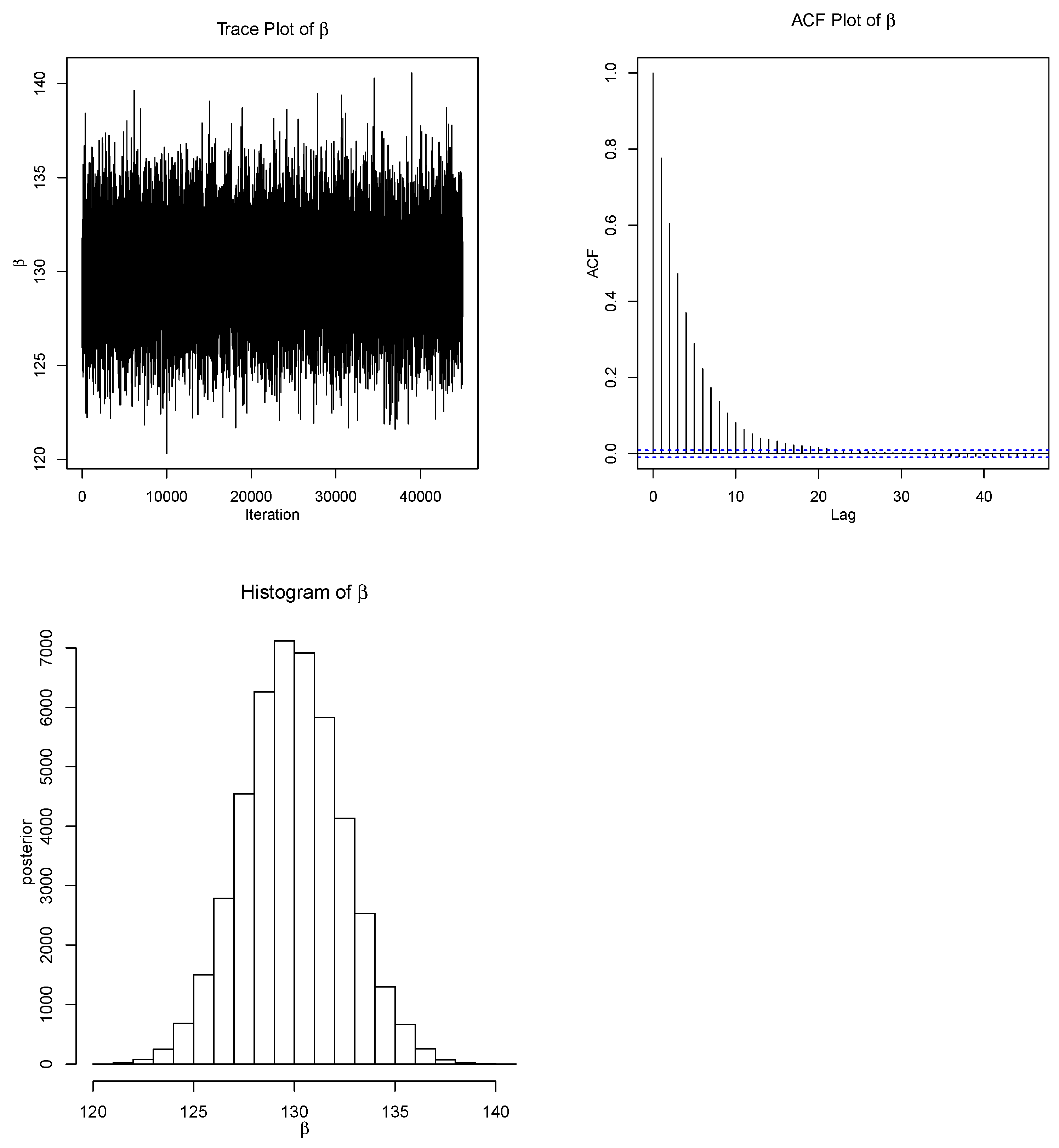Note that since we do not have any prior knowledge about the data, we assume that the priors are improper (precisely, $a_1=b_1=a_2=b_2=0$) to compute BEs and HPD CIs. The M–H algorithm is also employed to calculate the BEs of $\beta$. The Gaussian distribution is an adequate proposal distribution for the full conditional distribution of $\beta$, as clearly shown by Figure 2. Then, we can pick out the parameters of the proposal distribution to determine the best fitted model for the full conditional distribution. As a result, we use the M–H technique with the Gaussian proposal model to generate samples from the target probability distribution. Our natural choice of the initial value of $\beta$ is its MLE (${\widehat{\beta }}_M$), which is computed using the Newton–Raphson method, while the variance of $\beta$ is the reciprocal of the Fisher information, which is $S_{\beta }^2=5.960009$. We then generate $50,000$ random variates with $S_{\beta }^2=5.960009$ and find that the acceptance rate for this choice of variance is $71.03\%$, which is quite favorable. We burn in the initial 5000 samples and use the remaining observation to compute the BEs.

The trace and ACF plots are used effectively in checking the convergence of the M–H algorithm as a graphical diagnostic convergence tool. The trace and ACF plots for $\beta$ are shown in Figure 2. We can easily notice from the trace plot that there is a random scatter about a mean value represented by a solid line, with a fine mixing of the chains for the simulated values of $\beta$. We can also easily notice from the ACF plot that the autocorrelation of the chains is very low. Consequently, based on these plots, we can conclude that the M–H algorithm converges rapidly based on the proposed Gaussian distribution.

The outcomes for MLEs and BEs using importance and M–H samplers, in addition to the 95% Boot-t CI, asymptotic CI and HPD CI for $\alpha$ and $\beta$, are all displayed in

Table 1. Point estimates and 95% $CIs$ for $\alpha$ and $\beta$.

		SEL
m		MLE	Importance	M–H	Approximate CI	Boot-t CI	HPD CI
90	$\alpha$	0.1706	0.1769	0.1738	(0.1450, 0.1962)	(0.1465, 0.1967)	(0.1407, 0.1739)
	$\beta$	131.8776	132.2340	130.9982	(127.4480, 136.3064)	(127.5583, 135.8003)	(127.0845, 134.9120)
70	$\alpha$	0.1735	0.1787	0.1762	(0.1423, 0.2008)	(0.1446, 0.1989)	(0.1462, 0.1857)
	$\beta$	132.1070	132.3581	131.7418	(126.7428, 136.9137)	(126.7720, 136.0554)	(128.1083, 136.6701)

.

Now, we consider the prediction of some of the unseen values. The point predicted values and PIs for unseen values are computed as presented in

Table 2. Point predictors and 95% PIs of censored observations based on Bayesian methods.

		Point Predictors		PIs
		Importance	M–H	Importance	M–H
m = 90	n
	$Y_{1:11}$	162.67	162.18	(162.35, 163.52)	(161.75, 162.71)
	$Y_{2:11}$	166.23	163.65	(165.87, 167.12)	(163.36, 164.34)
	$Y_{3:11}$	169.68	166.16	(169.27, 170.93)	(165.95, 166.97)
	$Y_{4:11}$	173.05	170.61	(172.91, 174.61)	(170.14, 171.18)
	$Y_{5:11}$	179.83	174.70	(179.15, 180.86)	(179.38, 180.45)
	$Y_{6:11}$	187.14	180.22	(186.85, 188.62)	(179.88, 180.99)
	$Y_{7:11}$	196.41	187.85	(195.74, 197.52)	(187.63, 188.78)
	$Y_{8:11}$	204.38	195.79	(204.18, 205.97)	(195.42, 196.61)
	$Y_{9:11}$	211.27	204.16	(210.86, 212.68)	(203.33, 204.54)
	$Y_{10:11}$	217.02	213.06	(216.20, 218.06)	(212.35, 213.59)
m = 70	n
	$Y_{1:31}$	142.92	142.36	(142.12, 143.44)	(141.87, 143.07)
	$Y_{4:31}$	145.64	144.39	(144.92, 146.30)	(143.93, 145.16)
	$Y_{7:31}$	148.78	147.68	(148.06, 149.47)	(146.83, 148.11)
	$Y_{10:31}$	150.93	150.51	(150.23, 151.70)	(149.22, 150.54)
	$Y_{13:31}$	154.12	153.14	(153.64, 155.17)	(152.02, 153.38)
	$Y_{16:31}$	158.34	156.75	(157.51, 159.12)	(155.81, 157.22)
	$Y_{19:31}$	162.95	160.45	(162.33, 164.01)	(159.72, 161.18)
	$Y_{22:31}$	165.44	164.80	(164.19, 165.93)	(164.03, 165.52)
	$Y_{25:31}$	169.38	167.65	(168.48, 170.31)	(166.59, 168.14)
	$Y_{28:31}$	173.19	169.28	(171.86, 173.81)	(168.65, 170.28)

. The PIs are constructed under ab SEL function based on importance and M–H algorithms, the details of which are presented in Section 4. We can easily notice that the PIs established based on the M–H algorithm have the shortest intervals for all cases.

5.2. Simulation Results

Now, we use Monte Carlo simulation to compare the execution of the different estimation and prediction methods presented in the previous sections. We use bias and mean square error (MSE) criteria to compare the performance of the MLEs and BEs. In this simulation, we set the values of the parameters of BS to ($\alpha =2$, $\beta =1.5$) and ($\alpha =1.5$, $\beta =1.0$). Additionally, we consider different censoring schemes, along with different effective sample sizes of $n=25,50$ and 100. To perform the Bayesian analysis effectively, we assume three different priors. For prior 0, i.e., improper prior information, the prior parameters are assumed to take zero values of $a_1=b_1=a_2=b_2=0$. Next, two additional proper priors are assumed with same means but different variances to mirror the sensitivity of our inference to variations in the specification of prior parameters. Consequently, prior 1 and prior 2 are assumed to be $a_1=a_2=3,b_1=b_2=1$ and $a_1=a_2=5,b_1=b_2=2$, respectively. In this setting, prior 2 is more informative than prior 1. This enables us to evaluate the extent to which the informative prior contributes to the outcomes achieved based on observed values.

Table 3. (a) AWs and CPs of 95% CIs when $\alpha =2$ and $\beta =1.5$; (b) AWs and CPs of 95% CIs when $\alpha =1.5$ and $\beta =1.0$.

(a)
			Boot-t CI	Approximate CI	HPD CRI
CSs					Prior 0	Prior 1	Prior 2
$(25,15)$	$\alpha$	AW	2.2517	2.3739	1.9514	1.8017	1.7232
		CP	0.9317	0.9305	0.9344	0.9349	0.9412
	$\beta$	AW	1.7414	1.8509	1.6541	1.6247	1.5132
		CP	0.9423	0.9414	0.9450	0.9461	0.9485
$(25,20)$	$\alpha$	AW	2.1966	2.2978	1.8705	1.7751	1.6821
		CP	0.9327	0.9315	0.9352	0.9365	0.9425
	$\beta$	AW	1.7270	1.7962	1.5932	1.5701	1.4904
		CP	0.9431	0.9421	0.9459	0.9472	0.9494
$(50,30)$	$\alpha$	AW	2.0914	2.1885	1.8180	1.7237	1.6460
		CP	0.9333	0.9322	0.9357	0.9378	0.9425
	$\beta$	AW	1.6916	1.7351	1.5566	1.5202	1.4721
		CP	0.9438	0.9427	0.9466	0.9481	0.9504
$(50,40)$	$\alpha$	AW	1.9914	2.0805	1.7218	1.6191	1.5446
		CP	0.9384	0.9377	0.9404	0.9418	0.9448
	$\beta$	AW	1.5538	1.6101	1.4912	1.4593	1.4119
		CP	0.9457	0.9446	0.9473	0.9492	0.9510
(b)
			Boot-t CI	Approximate CI	HPD CRI
CSs					Prior 0	Prior 1	Prior 2
$(100,50)$	$\alpha$	AW	1.8513	1.9223	1.6289	1.5094	1.4650
		CP	0.9407	0.9399	0.9427	0.9438	0.9490
	$\beta$	AW	1.4461	1.5338	1.3936	1.3527	1.3121
		CP	0.9470	0.9461	0.9483	0.9501	0.9519
$(100,75)$	$\alpha$	AW	1.6332	1.7618	1.5059	1.4639	1.4012
		CP	0.9422	0.9409	0.9440	0.9462	0.9499
	$\beta$	AW	1.2736	1.3812	1.2094	1.1509	1.4220
		CP	0.9479	0.9470	0.9491	0.9512	0.9523
$(100,90)$	$\alpha$	AW	1.4418	1.5642	1.3601	1.3025	1.2180
		CP	0.9431	0.9420	0.9449	0.9468	0.9513
	$\beta$	AW	1.0799	1.1846	0.9878	0.9222	0.8709
		CP	0.9488	0.9482	0.9504	0.9519	0.9530
$(25,15)$	$\alpha$	AW	1.1287	1.1745	1.0749	1.0165	0.9624
		CP	0.9267	0.9249	0.9277	0.9289	0.9298
	$\beta$	AW	0.7641	0.8185	0.7141	0.6722	0.6104
		CP	0.9377	0.9363	0.9389	0.9396	0.9405
$(25,20)$	$\alpha$	AW	1.0628	1.1151	0.9856	0.9346	0.8957
		CP	0.9277	0.9261	0.9284	0.9293	0.9303
	$\beta$	AW	0.7338	0.7848	0.6984	0.6325	0.5974
		CP	0.9388	0.9372	0.9397	0.9406	0.9414
$(50,30)$	$\alpha$	AW	0.9792	1.0244	0.9184	0.8771	0.8263
		CP	0.9285	0.9273	0.9290	0.9298	0.9311
	$\beta$	AW	0.7269	0.7674	0.6752	0.6184	0.5841
		CP	0.9398	0.9387	0.9410	0.9421	0.9433
$(50,40)$	$\alpha$	AW	0.9176	0.9714	0.8768	0.8322	0.7968
		CP	0.9296	0.9285	0.9305	0.9312	0.9324
	$\beta$	AW	0.7055	0.7354	0.6554	0.6065	0.5692
		CP	0.9409	0.9401	0.9425	0.9438	0.9449
$(100,50)$	$\alpha$	AW	0.8620	0.9109	0.8224	0.7889	0.7405
		CP	0.9310	0.9299	0.9321	0.9327	0.9339
	$\beta$	AW	0.6908	0.7115	0.6381	0.5812	0.5534
		CP	0.9427	0.9419	0.9441	0.9453	0.9467
$(100,75)$	$\alpha$	AW	0.8119	0.8569	0.7751	0.7396	0.7008
		CP	0.9326	0.9312	0.9342	0.9359	0.9372
	$\beta$	AW	0.6684	0.6912	0.6119	0.5687	0.5404
		CP	0.9443	0.9437	0.9458	0.9470	0.9481
$(100,90)$	$\alpha$	AW	0.7668	0.8077	0.7259	0.6961	0.6643
		CP	0.9343	0.9329	0.9361	0.9384	0.9398
	$\beta$	AW	0.6178	0.6546	0.5961	0.5413	0.5176
		CP	0.9462	0.9455	0.9476	0.9489	0.9499

presents the average widths (AWs) and coverage probabilities (CPs) of 95% CIs for $\alpha$ and $\beta$ based on Boot-t, asymptotic ML and Bayesian methods with the improper prior (prior 0) and informative priors (prior 1 and prior 2) under the SEL function. For 10,000 replications, the average bias and MSEs of the MLEs and BEs under the SEL of $\alpha$ and $\beta$ are computed as displayed in

Table 4. (a) Bias and MSEs of the MLEs and BEs when $\alpha =2$ and $\beta =1.5$; (b) Bias and MSEs of the MLEs and BEs when $\alpha =1.5$ and $\beta =1.0$.

(a)
		MLE		Prior 0		Prior 1		Prior 2
CSs↓		Bias	MSE	Bias	MSE	Bias	MSE	Bias	MSE
$(25,15)$	$\alpha$	0.5877	0.6634	−0.5362	0.6185	0.4581	0.5852	0.4208	0.5646
	$\beta$	0.6293	0.8816	0.5863	0.8205	0.5814	0.7848	0.5747	0.7659
$(25,20)$	$\alpha$	0.5615	0.6618	−0.5199	0.6138	0.4521	0.5832	0.4199	0.5629
	$\beta$	−0.6220	0.8758	0.5848	0.8095	0.5757	0.7765	0.5687	0.7593
$(50,30)$	$\alpha$	0.5558	0.6578	−0.5034	0.6114	0.4456	0.5793	0.4039	0.5577
	$\beta$	0.6142	0.8681	0.5803	0.7883	0.5741	0.7698	0.5647	0.7469
$(50,40)$	$\alpha$	0.5508	0.6507	−0.4984	0.6075	0.4361	0.5689	0.4004	0.5467
	$\beta$	0.6072	0.8577	0.5752	0.7778	0.5644	0.7602	−0.5604	0.7366
$(100,50)$	$\alpha$	0.5422	0.6481	0.4901	0.5911	0.4288	0.5541	0.3986	0.5371
	$\beta$	0.5994	0.8419	0.5721	0.7642	0.5684	0.7567	−0.5585	0.7287
$(100,75)$	$\alpha$	−0.5328	0.6342	−0.4862	0.5817	0.4194	0.5456	0.3934	0.5308
	$\beta$	0.5916	0.8221	0.5895	0.7475	0.5686	0.7390	−0.5524	0.7118
$(100,90)$	$\alpha$	−0.5378	0.6216	−0.4807	0.5739	0.4128	0.5359	0.3912	0.5252
	$\beta$	0.5888	0.7932	0.5805	0.7152	0.5642	0.6789	−0.5493	0.6518
(b)
		MLE		Prior 0		Prior 1		Prior 2
CSs↓		Bias	MSE	Bias	MSE	Bias	MSE	Bias	MSE
$(25,15)$	$\alpha$	−0.5214	0.5836	0.4835	0.5523	−0.4466	0.5254	0.4087	0.4978
	$\beta$	0.5417	0.7336	0.5263	0.6877	0.5183	0.6564	−0.5022	0.6328
$(25,20)$	$\alpha$	0.5068	0.5687	−0.4682	0.5363	0.4322	0.5081	0.3951	0.4795
	$\beta$	0.5359	0.7167	0.5177	0.6744	0.5089	0.6412	0.5002	0.6202
$(50,30)$	$\alpha$	0.4892	0.5522	0.4543	0.5207	−0.4262	0.4924	0.3849	0.4629
	$\beta$	−0.5246	0.6867	0.5119	0.6379	−0.4987	0.6184	0.4921	0.5962
$(50,40)$	$\alpha$	−0.4773	0.5419	0.4408	0.5067	0.4171	0.4761	−0.3762	0.4473
	$\beta$	−0.5061	0.6715	0.4970	0.6226	0.4831	0.6033	−0.4768	0.5829
$(100,50)$	$\alpha$	0.4685	0.5269	0.4278	0.4933	0.4103	0.4612	0.3679	0.4340
	$\beta$	0.4924	0.6547	−0.4856	0.6106	−0.4752	0.5942	0.4635	0.5718
$(100,75)$	$\alpha$	−0.4433	0.5157	0.4116	0.4793	0.3965	0.4536	−0.3539	0.4258
	$\beta$	0.4782	0.6387	−0.4668	0.6036	0.4572	0.5834	−0.4513	0.5611
$(100,90)$	$\alpha$	0.4318	0.4962	−0.4032	0.4674	0.3722	0.4426	−0.3469	0.4130
	$\beta$	0.4637	0.6247	0.4528	0.5886	−0.4450	0.5657	0.4377	0.5462

a,b. We observe from Table 3a,b that the HPD CIs are shorter than the asymptotic and Boot-t CIs under all priors for $n=25,50,100$ with different values of m. The performance of HPD CIs tends to be higher under informative priors than that of the asymptotic and Boot-t CIs. The Boot-t method performs well when compared to the asymptotic method in terms of estimating all parameters. It can also be noticed that when n increases, all CI types tend to become shorter. The simulated CPs are very close to each other for all these CIs. As shown in Table 4a,b, in terms of bias and MSEs, the BEs perform well for all values of n and m. For all sample sizes, we can notice that the Bayesian estimates of $\alpha$ and $\beta$ are better than the MLEs, as indicated by their lower bias and MSEs compared to MLE results. Additionally, as expected, we can notice that the BEs under the more informative prior 2 are better than the less informative and non-informative priors. Finally, we can clearly conclude that the results of BEs are sensitive to the presumed values of the prior parameters, specifically for the informative prior (prior 2).

For the prediction problem, different type-II censored schemes are randomly generated from the BS model and for $n=25,50,100$. Then, the average bias and mean square prediction errors (MSPEs) are computed for the predictors and PIs for censored times. The bias and MSPEs of BPs are computed over 10,000 replications for non-informative and informative priors. The values of the bias and MSPEs are reported in

Table 5. Bias and MSPEs of BPs for censored units when $\alpha =2$ and $\beta =1.5$.

			Prior 0		Prior 1		Prior 2
CSs			Importance	M–H	Importance	M–H	Importance	M–H
	$Y_{1:10}$	Bias	0.4927	−0.4718	−0.4727	0.4558	0.4582	0.4414
$(25,15)$		MSPE	0.9638	0.9035	0.9287	0.8778	0.8536	0.7928
	$Y_{3:10}$	Bias	0.5225	0.5064	−0.4958	0.4726	0.4784	−0.4567
		MSPE	0.9839	0.9189	0.9682	0.8965	0.9318	0.8590
	$Y_{7:10}$	Bias	0.5754	−0.5419	0.5234	0.5012	0.4935	−0.4731
		MSPE	0.9986	0.9376	0.9712	0.9094	0.9515	0.8708
	$Y_{10:10}$	Bias	−0.6254	0.5659	0.6060	0.5422	0.5664	0.5033
		MSPE	1.1903	0.9653	0.9925	0.9312	0.9674	0.8851
	$Y_{1:5}$	Bias	−0.4706	0.4553	0.4471	0.4232	0.4269	−0.4061
$(25,20)$		MSPE	0.9329	0.8874	0.8844	0.8375	0.8385	0.7862
	$Y_{3:5}$	Bias	0.4829	0.4646	0.4617	0.4351	0.4473	−0.4129
		MSPE	0.9452	0.8963	0.8987	0.8566	0.8450	0.7921
	$Y_{5:5}$	Bias	−0.4992	0.4741	0.4836	0.4454	0.4692	−0.4235
		MSPE	0.9556	0.9048	0.9116	0.8648	0.8509	0.8092
	$Y_{1:20}$	Bias	0.4595	0.4331	−0.4327	0.4119	0.4180	0.3968
$(50,30)$		MSPE	0.9065	0.8421	0.8562	0.8072	0.7945	0.7554
	$Y_{5:20}$	Bias	−0.4762	0.4571	0.4558	−0.4309	0.4397	0.4098
		MSPE	0.9267	0.8690	0.8829	0.8348	0.8201	0.7860
	$Y_{10:20}$	Bias	−0.4956	0.4676	0.4879	0.4480	0.4722	0.4213
		MSPE	0.9445	0.8905	0.9014	0.8536	0.8562	0.7965
	$Y_{15:20}$	Bias	0.5206	0.4882	−0.5063	0.4685	0.4885	0.4399
		MSPE	0.9766	0.9231	0.93725	0.8761	0.8964	0.8260
	$Y_{20:20}$	Bias	−0.5451	0.4923	0.5268	0.4767	−0.5016	0.4456
		MSPE	0.9966	0.9586	0.9782	0.9077	0.9375	0.8563
	$Y_{1:10}$	Bias	0.4406	−0.4193	0.4185	0.3933	−0.3946	0.3739
$(50,40)$		MSPE	0.8725	0.7917	0.8229	0.7724	0.7642	0.7311
	$Y_{3:10}$	Bias	0.4569	−0.4216	0.4332	0.4094	−0.4243	0.3817
		MSPE	0.8962	0.8248	0.8536	0.7968	0.8047	0.7552
	$Y_{7:10}$	Bias	0.4765	−0.4374	0.4518	0.4147	−0.4386	−0.3984
		MSPE	0.9261	0.8560	0.8825	0.8485	0.8492	0.7946
	$Y_{10:10}$	Bias	0.4980	0.4516	0.4753	0.4276	0.4522	−0.4058
		MSPE	0.9508	0.8971	0.9360	0.8740	0.9313	0.8421
	$Y_{1:50}$	Bias	−0.4357	0.4031	0.4046	0.3802	0.3847	0.3631
$(100,50)$		MSPE	0.8270	0.7228	0.8069	0.7089	0.7226	0.6852
	$Y_{10:50}$	Bias	0.4524	0.4275	0.4215	−0.4082	0.4077	0.3829
		MSPE	0.8533	0.7438	0.8366	0.7475	0.7896	0.7355
	$Y_{20:50}$	Bias	0.4713	0.4386	−0.4462	0.4123	−0.4227	0.3907
		MSPE	0.8952	0.8205	0.8692	0.8067	0.8459	0.7847
	$Y_{30:50}$	Bias	−0.4982	0.4448	0.4615	0.4227	0.4462	−0.4079
		MSPE	0.9568	0.8750	0.9187	0.8592	0.8852	0.8356
	$Y_{40:50}$	Bias	0.5095	0.4547	0.4791	0.4313	0.4562	0.4175
		MSPE	0.9971	0.9467	0.9563	0.9168	0.9048	0.8653
	$Y_{50:50}$	Bias	0.5252	−0.4740	0.4962	0.4515	0.4708	−0.4356
		MSPE	1.0964	0.9806	1.0167	0.9551	0.9719	0.9046
	$Y_{1:25}$	Bias	−0.4052	0.3761	0.3771	0.3356	0.3582	0.3174
$(100,75)$		MSPE	0.7849	0.7007	0.7584	0.6848	0.6938	0.6692
	$Y_{10:25}$	Bias	0.4450	0.3952	0.4097	0.3563	−0.3816	0.3373
		MSPE	0.8253	0.7709	0.7967	0.7264	0.7510	0.6980
	$Y_{20:25}$	Bias	−0.4758	0.4136	0.4352	0.3866	−0.4127	0.3588
		MSPE	0.8676	0.8471	0.8479	0.7812	0.8052	0.7249
	$Y_{25:25}$	Bias	0.4937	0.4311	−0.4632	0.4059	0.4367	−0.3742
		MSPE	0.9081	0.8689	0.8630	0.8351	0.8471	0.7763
	$Y_{1:10}$	Bias	−0.3869	0.3577	0.3550	−0.3177	0.3378	0.2981
$(100,90)$		MSPE	0.7255	0.6544	0.7065	0.6462	0.6552	0.6269
	$Y_{3:10}$	Bias	−0.4052	0.3650	0.3798	−0.3262	−0.3515	0.3074
		MSPE	0.7789	0.6837	0.7467	0.6641	0.6985	0.6480
	$Y_{7:10}$	Bias	−0.4259	0.3831	0.3954	0.3468	0.3722	0.3281
		MSPE	0.7965	0.7188	0.7713	0.6812	0.7461	0.6749
	$Y_{10:10}$	Bias	0.4537	0.4022	−0.4239	0.3661	0.3953	−0.3440
		MSPE	0.8312	0.7485	0.7963	0.7035	0.7713	0.6993

and

Table 6. Bias and MSPEs of BPs for censored units when $\alpha =1.5$ and $\beta =1.0$.

			Prior 0		Prior 1		Prior 2
CSs			Importance	M–H	Importance	M–H	Importance	M–H
	$Y_{1:10}$	Bias	0.4566	0.4186	−0.4425	0.4101	0.4355	−0.4031
$(25,15)$		MSPE	0.8114	0.7424	0.8059	0.7348	0.7968	0.7228
	$Y_{5:10}$	Bias	0.4733	0.4291	0.4625	0.4207	0.4589	0.4116
		MSPE	0.8365	0.7574	0.8221	0.7486	0.8133	0.7357
	$Y_{10:10}$	Bias	0.4917	0.4390	0.4886	0.4282	−0.4739	0.4189
		MSPE	0.8520	0.7691	0.8406	0.7612	0.8311	0.7486
	$Y_{1:5}$	Bias	0.4683	−0.4274	−0.4442	−0.4155	0.4262	0.4012
$(25,20)$		MSPE	0.7952	0.7289	0.7872	0.7193	0.7786	0.7115
	$Y_{3:5}$	Bias	0.4828	0.4438	0.4594	0.4208	0.4382	−0.4087
		MSPE	0.8108	0.7385	0.8023	0.7226	0.7983	0.7179
	$Y_{5:5}$	Bias	−0.5037	0.4556	0.4728	0.4372	0.4558	−0.4154
		MSPE	0.9556	0.7458	0.9116	0.7321	0.8509	0.7249
	$Y_{1:20}$	Bias	−0.4336	0.3923	0.4258	0.3852	0.4122	−0.3721
$(50,30)$		MSPE	0.7728	0.7033	0.7619	0.6927	0.7542	0.6886
	$Y_{10:20}$	Bias	0.4585	−0.4135	0.4448	−0.4089	0.4325	0.3942
		MSPE	0.7862	0.7086	0.7741	0.7018	0.7639	0.6952
	$Y_{20:20}$	Bias	−0.4736	−0.4392	0.4682	0.4282	−0.4567	0.4122
		MSPE	0.7958	0.7224	0.7854	0.7166	0.7741	0.7052
	$Y_{1:10}$	Bias	0.4293	0.3858	0.4015	0.3643	0.3855	0.3597
$(50,40)$		MSPE	0.7346	0.6625	0.7162	0.6433	0.7016	0.6331
	$Y_{5:10}$	Bias	0.4381	0.3951	−0.4139	0.3779	0.3974	0.3686
		MSPE	0.7406	0.6864	0.7324	0.6741	0.7152	0.6576
	$Y_{10:10}$	Bias	0.4532	0.4120	0.4294	0.3906	−0.4107	0.3775
		MSPE	0.7745	0.7154	0.7486	0.6986	0.7374	0.6693
	$Y_{1:25}$	Bias	0.3828	−0.3569	−0.3766	0.3458	0.3615	0.3346
$(100,75)$		MSPE	0.6589	0.5962	0.6413	0.5832	0.6280	0.5673
	$Y_{13:25}$	Bias	0.4063	−0.3779	0.3951	0.3665	0.3878	0.3532
		MSPE	0.7066	0.6382	0.6871	0.6119	0.5714	0.5879
	$Y_{25:25}$	Bias	0.4180	−0.3913	0.4096	0.3857	−0.3961	−0.3677
		MSPE	0.7668	0.6893	0.7503	0.6680	0.7387	0.6459
	$Y_{1:10}$	Bias	−0.3397	0.3067	0.3265	0.2854	0.3159	0.2678
$(100,90)$		MSPE	0.6158	0.5437	0.6008	0.5216	0.5837	0.5076
	$Y_{5:10}$	Bias	0.3518	0.3196	−0.3381	0.2955	0.3292	−0.2779
		MSPE	0.6374	0.5722	0.6192	0.5594	0.6083	0.5280
	$Y_{10:10}$	Bias	0.3782	0.3346	0.3591	−0.3083	0.3511	0.2936
		MSPE	0.6733	0.6011	0.6527	0.5738	0.6339	0.5458

for the predetermined censoring schemes.

Table 7. AWs and CPs of PIs for censored units based on importance, M–H and Boot-t samplers when $\alpha =2$ and $\beta =1.5$.

CSs
$n=25$		$Y_{1:10}$	$Y_{3:10}$	$Y_{7:10}$	$Y_{10:10}$	-	-
$m=15$	Boot-t	2.2455 (0.9552)	2.5622 (0.9532)	2.7956 (0.9514)	2.9261 (0.9493)	-	-
	Importance	1.9832 (0.9590)	2.2071 (0.9577)	2.4747 (0.9553)	2.6437 (0.9531)	-	-
	M–H	1.7878 (0.9634)	1.9144 (0.9617)	2.1528 (0.9596)	2.2952 (0.9580)	-	-
$n=25$		$Y_{1:5}$	$Y_{3:5}$	$Y_{5:5}$	-	-	-
$m=20$	Boot-t	2.1034 (0.9541)	2.2858 (0.9522)	2.4235 (0.9509)	-	-	-
	Importance	1.8235 (0.9569)	2.0486 (0.9548)	2.1962 (0.9537)	-	-	-
	M–H	1.7168 (0.9619)	1.8330 (0.9602)	1.9553 (0.9589)	-	-	-
$n=50$		$Y_{1:20}$	$Y_{5:20}$	$Y_{10:20}$	$Y_{15:20}$	$Y_{20:20}$	-
$m=30$	Boot-t	1.9202 (0.9521)	2.1908 (0.9508)	2.3212 (0.9488)	2.5113 (0.9472)	2.6883 (0.9457)	-
	Importance	1.7591 (0.9579)	1.8105 (0.9564)	1.9368 (0.9549)	2.0827 (0.9534)	2.1971 (0.9521)	-
	M–H	1.6044 (0.9585)	1.7020 (0.9573)	1.8218 (0.9562)	1.9654 (0.9549)	2.1340 (0.9537)	-
$n=50$		$Y_{1:10}$	$Y_{3:10}$	$Y_{7:10}$	$Y_{10:10}$	-	-
$m=40$	Boot-t	1.7352 (0.9508)	1.8547 (0.9487)	1.9252 (0.9471)	2.1624 (0.9460)	-	-
	Importance	1.5765 (0.9563)	1.6675 (0.9549)	1.7428 (0.9535)	1.9098 (0.9523)	-	-
	M–H	1.2809 (0.9574)	1.4270 (0.9562)	1.5151 (0.9550)	1.6443 (0.9542)	-	-
$n=100$		$Y_{1:50}$	$Y_{10:50}$	$Y_{20:50}$	$Y_{30:50}$	$Y_{40:50}$	$Y_{50:50}$
$m=50$	Boot-t	1.5937 (0.9492)	1.7908 (0.9479)	1.9655 (0.9464)	2.1903 (0.9451)	2.3765 (0.9438)	2.5826 (0.9425)
	Importance	1.3866 (0.9547)	1.5624 (0.9533)	1.7139 (0.9519)	1.8608 (0.9505)	1.9890 (0.9487)	2.1423 (0.9465)
	M–H	1.2921 (0.9558)	1.4002 (0.9549)	1.5520 (0.9534)	1.7292 (0.9520)	1.8937 (0.9511)	2.0282 (0.9497)
$n=100$		$Y_{1:25}$	$Y_{10:25}$	$Y_{20:25}$	$Y_{25:25}$	-	-
$m=75$	Boot-t	1.4652 (0.9478)	1.6254 (0.9466)	1.8429 (0.9453)	1.9492 (0.9441)	-	-
	Importance	1.2236 (0.9521)	1.4351 (0.9511)	1.6023 (0.9496)	1.7385 (0.9485)	-	-
	M–H	1.1305 (0.9532)	1.2824 (0.9523)	1.4325 (0.9510)	1.5027 (0.9496)	-	-
$n=100$		$Y_{1:10}$	$Y_{3:10}$	$Y_{7:10}$	$Y_{10:10}$	-	-
$m=90$	Boot-t	1.2652 (0.9460)	1.3824 (0.9446)	1.4629 (0.9431)	1.5492 (0.9418)	-	-
	Importance	1.0952 (0.9508)	1.2251 (0.9485)	1.3423 (0.9471)	1.4138 (0.9556)	-	-
	M–H	0.8505 (0.9517)	0.9824 (0.9504)	1.1482 (0.9484)	1.2627 (0.9471)	-	-

and

Table 8. AWs and CPs of PIs for censored units based on importance, M–H and Boot-t samplers when $\alpha =1.5$ and $\beta =1.0$.

CSs
$n=25$		$Y_{1:10}$	$Y_{5:10}$	$Y_{10:10}$
$m=15$	Boot-t	1.8862 (0.9528)	1.9374 (0.9512)	2.2138 (0.9501)
	Importance	1.6974 (0.9545)	1.8062 (0.9533)	1.9318 (0.9520)
	M–H	1.5217 (0.9571)	1.6682 (0.9553)	1.7991 (0.9533)
$n=25$		$Y_{1:5}$	$Y_{3:5}$	$Y_{5:5}$
$m=20$	Boot-t	1.7605 (0.9516)	1.8426 (0.9504)	1.9571 (0.9490)
	Importance	1.6033 (0.9532)	1.7283 (0.9519)	1.8479 (0.9509)
	M–H	1.4880 (0.9547)	1.6046 (0.9535)	1.7379 (0.9522)
$n=50$		$Y_{1:20}$	$Y_{10:20}$	$Y_{20:20}$
$m=30$	Boot-t	1.6254 (0.9502)	1.7533 (0.9489)	1.8438 (0.9473)
	Importance	1.5039 (0.9517)	1.6117 (0.9504)	1.6995 (0.9491)
	M–H	1.3906 (0.9530)	1.5056 (0.9518)	1.5927 (0.9505)
$n=50$		$Y_{1:10}$	$Y_{5:10}$	$Y_{10:10}$
$m=40$	Boot-t	1.4995 (0.9488)	1.6228 (0.9475)	1.7168 (0.9462)
	Importance	1.3455 (0.9498)	1.4570 (0.9487)	1.5617 (0.9474)
	M–H	1.2018 (0.9515)	1.2984 (0.9504)	1.4118 (0.9492)
$n=100$		$Y_{1:25}$	$Y_{13:25}$	$Y_{25:25}$
$m=75$	Boot-t	1.3161 (0.9459)	1.4471 (0.9446)	1.5682 (0.9432)
	Importance	1.1535 (0.9472)	1.2659 (0.9460)	1.3829 (0.9446)
	M–H	1.0259 (0.9488)	1.1138 (0.9474)	1.2492 (0.9461)
$n=100$		$Y_{1:10}$	$Y_{5:10}$	$Y_{10:10}$
$m=90$	Boot-t	1.1788 (0.9443)	1.2958 (0.9430)	1.3823 (0.9418)
	Importance	1.0209 (0.9457)	1.1327 (0.9444)	1.2273 (0.9430)
	M–H	0.8027 (0.9469)	0.8912 (0.9460)	0.9798 (0.9448)

include the AWs and CPs of $95\%$ PIs based on importance, M–H and Boot-t. It can be noticed from Table 5 and Table 6 that the BPs using the M–H method perform well compared to the importance sampler method in terms of the reported values of bias and MSPE for all priors. It is observed for all sample sizes that both importance sampling and M–H methods perform well under the more informative prior 2 than those using the less informative or non-informative priors, with obvious privilege for the M–H method due to its lower bias and MSPE values. As foreseen, when m increases, the MSPEs of the censored times tend to be larger due to the increase in the quantity of observed data. From Table 7 and Table 8, in terms of the AW criterion, a clear clue can be observed that supports the conclusion that the Bayesian PIs based on M–H sampling are the best PIs. We can also noticed that the PIs calculated using importance sampling perform better than those calculated using the Boot-t method based on the reported AW values. Furthermore, as anticipated, the farther the censored value is from the last observed value, the larger the AW values are compared to those that are closer. The CP values are close to each other. It can also be seen that the Bayesian PIs under the informative prior (prior 2) behave better than PIs based on other priors. Furthermore, the simulated CPs are high and tend to be close to the accurate prediction coefficient ($1-\gamma =0.95$).

6. Discussion and Conclusions

In this study, we investigated parameter estimation and prediction methods for type-II censored BS data. We compared frequentist and Bayesian approaches, employing MCMC sampling to estimate parameters and construct credible intervals. Our results shows that that two methods provide comparable estimates for the shape and scale parameters. The Bayesian method provides more reliable and flexible prediction intervals compared to classical methods, especially when prior information is available. By applying these methods to simulated and real-world data, we have shown the practical advantage of the presented approaches in reliability and survival analysis.

Failure data, like the fatigue life of materials, are of credible interest in reliability analysis. Therefore, methods based on degradation data are increasingly common in industries such as manufacturing, healthcare and materials science. When the process leading to failure is slow or progressive with deteriorating performance over time, degradation data models are usually used. These models can employed effectively to better understanding how a product or system degrades before it fails, including through the use of functional models, stochastic processes and random-effects models.

Ruiz et al. [28], Zhai et al. [29], and Xu et al. [30], among others, have recently focused on using degradation models to evaluate product reliability. For example, Ruiz et al. [28] introduced generalized functional mixed models for accelerated degradation testing, which allowed them to predict failure times accurately by modeling the degradation process under stress. Zhai et al. [29] suggested a random-effects Wiener process approach to model product degradation with heterogeneity, considering the variability between products that may fail at different rates. Similarly, Xu et al. [30] developed a multivariate Student-t process model for degradation data with tail-weighted distributions to study common problems in industrial reliability.

Our current study mainly focuses on failure time data under type-II censoring, where the data represent the times at which components fail under stress or other conditions. The two approaches are applied in different contexts. The main advantage of degradation models is their ability to model the gradual deterioration of products, which allows for more careful estimations of remaining beneficial life before failure occurs. On the contrary, failure time analysis under type-II censoring is more convenient when data are collected after a certain number of failures have been observed. This makes it ideal for situations where products are tested to failure.

There is a clear possibility that future research will integrate these models with type-II censoring, as our current methods do not directly associate degradation data models. This combination might provide more accurate and comprehensive reliability assessments, especially when there is a relationship between failure times and degradation patterns for some products. By combining degradation modeling with the Bayesian approach used in this work, we could offer a more flexible and deep approach to handling both types of data, which, in turn, can enable better predictions of the possible failure times of a product based on its degradation path.

Moreover, this study provides valuable insights into parameter estimation and prediction using type-II censored BS data. However, the growing importance of degradation data models in reliability analysis calls for further consideration of how these models can be integrated with our presented methods. Future promising work will study these extensions, as well as the application of our methods to larger datasets, multi-sample progressive censoring schemes and industrial applications involving degradation data.

References

1. Birnbaum, Z.W.; Saunders, S.C. A new family of life distribution. J. Appl. Probab. 1969, 6, 319–327. [Google Scholar] [CrossRef]
2. Birnbaum, Z.W.; Saunders, S.C. Estimation for a family of life distributions with applications to fatigue. J. Appl. Probab. 1969, 6, 328–347. [Google Scholar] [CrossRef]
3. Desmond, A.F. Stochastic models of failure in random environments. Can. J. Stat. 1985, 13, 171–183. [Google Scholar] [CrossRef]
4. Langl, A.O.; Pocock, S.J.; Kerr, G.R.; Gore, S.M. Long-term survival of patients with breast cancer: A study of the curability of the disease. Br. Med. J. 1979, 2, 1247–1251. [Google Scholar] [CrossRef] [PubMed]
5. Balakrishnan, N.; Kundu, D. Birnbaum-Saunders distribution: A review of models, analyses, and applications. Appl. Stochastic. Models Bus Ind. 2019, 35, 4–132, (with discussions). [Google Scholar] [CrossRef]
6. Engelhardt, M.; Bain, L.J.; Wright, F.T. Inferences on the parameters of the Birnbaum-Saunders fatigue life distribution based on maximum likelihood estimation. Technometrics 1981, 23, 251–256. [Google Scholar] [CrossRef]
7. Balakrishnan, N.; Zhu, X. On the existence and uniqueness of the maximum likelihood estimates of parameters of Birnbaum-Saunders distribution based on Type-I, Type-II and hybrid censored samples. Statistics 2014, 48, 1013–1032. [Google Scholar] [CrossRef]
8. Ng, H.K.T.; Kundu, D.; Balakrishnan, N. Point and interval estimations for the two-parameter Birnbaum-Saunders distribution based on type-II censored samples. Comput. Stat. Data Anal. 2006, 50, 3222–3242. [Google Scholar] [CrossRef]
9. Padgett, W.J. On Bayes estimation of reliability for the Birnbaum-Saunders fatigue life model. IEEE Trans. Reliab. 1982, 31, 436–438. [Google Scholar] [CrossRef]
10. Achcar, J.A. Inferences for the Birnbaum-Saunders fatigue life model using Bayesian methods. Comput. Stat. Data Anal. 1993, 15, 367–380. [Google Scholar] [CrossRef]
11. Achcar, J.A.; Moala, F.A. Use of MCMC methods to obtain Bayesian inferences for the Birnbaum-Saunders distribution in the presence of censored data and covariates. Adv. Appl. Stat. 2010, 17, 1–27. [Google Scholar]
12. Wang, M.; Sun, X.; Park, C. Bayesian analysis of Birnbaum-Saunders distribution via the generalized ratio-of-uniforms method. Comput. Stat. 2016, 31, 207–225. [Google Scholar] [CrossRef]
13. Liu, Y.; Zhang, H.; Li, W. A novel random-effect Birnbaum-Saunders distribution for reliability assessment considering accelerated mechanism equivalence. Comput. Stat. 2024, 39, 501–515. [Google Scholar] [CrossRef]
14. Sawlan, Z.; Hasan, M.; Abdel-Mageed, R. Modeling metallic fatigue data using the Birnbaum-Saunders distribution. Fatigue Fract. Eng. Mater Struct. 2023, 46, 1423–1434. [Google Scholar] [CrossRef]
15. Razmkhah, M.; Karami, S.; Salim, S. Neutrosophic Birnbaum-Saunders distribution with applications. J. Stat. Comput. Simul. 2024, 94, 298–315. [Google Scholar]
16. Park, C.; Wang, M. A goodness-of-fit test for the Birnbaum-Saunders distribution based on the probability plot. Stat. Probabil. Lett. 2023, 174, 125–136. [Google Scholar]
17. Dorea, C.C.Y.; Silva, M.D.; Lima, G. A general class of fatigue-life distributions of Birnbaum-Saunders type. Reliab. Eng. Syst. Saf. 2023, 229, 108–118. [Google Scholar]
18. Kaminsky, K.S.; Nelson, P.I. Prediction of order statistics. In Handbook of Statistics: Order Statistics: Applications; Balakrishnan, N., Rao, C.R., Eds.; North-Holland: Amsterdam, The Netherlands, 1998; Volume 17, pp. 431–450. [Google Scholar]
19. Al-Hussaini, E.K. Predicting observable from a general class of distributions. J. Stat. Plan. Inference 1999, 79, 79–81. [Google Scholar] [CrossRef]
20. Kundu, D.; Raqab, M.Z. Bayesian inference and prediction of order statistics for type-II censored Weibull distribution. J. Stat. Plan. Inference 2012, 142, 41–47. [Google Scholar] [CrossRef]
21. Bdair, O.M.; Awwad, R.R.A.; Abufoudeh, G.K.; Naser, M.F.M. Estimation and prediction for flexible Weibull distribution based on progressive Type-II censored data. Commun. Math. Stat. 2020, 8, 255–277. [Google Scholar] [CrossRef]
22. Balakrishnan, N.; Cohen, A.C. Order Statistics and Inference: Estimation Methods; Academic Press: San Diego, CA, USA, 1991. [Google Scholar]
23. Ahmed, E.A. Bayesian estimation based on progressive Type-II censoring from two-parameter bathtub-shaped lifetime model: An Markov chain Monte Carlo approach. J. Appl. Stat. 2014, 41, 752–768. [Google Scholar] [CrossRef]
24. Tsay, W.J.; Huang, C.J.; Fu, T.T.; Ho, I.L. A simple closed-form approximation for the cumulative distribution function of the composite error of stochastic frontier models. J. Prod. Anal. 2013, 39, 259–269. [Google Scholar] [CrossRef]
25. Chen, M.H.; Shao, Q.M. Monte Carlo estimation of Bayesian credible and HPD intervals. J. Comput. Graph. Stat. 1999, 8, 69–92. [Google Scholar] [CrossRef]
26. Arnold, B.C.; Balakrishan, N.; Nagaraja, H.N. A First Course in Order Statistics; Wiley: New York, NY, USA, 1992. [Google Scholar]
27. Tierney, L. Markov chains for exploring posterior distributions. Ann. Stat. 1994, 22, 1701–1728. [Google Scholar] [CrossRef]
28. Ruiz, C.; Liao, H.; Pohl, E.A. Generalized Functional Mixed Models for Accelerated Degradation-Based Reliability Analysis. IEEE Trans. Reliab. 2024. [Google Scholar] [CrossRef]
29. Zhai, Q.; Li, Y.; Chen, P. Modeling Product Degradation with Heterogeneity: A General Random-Effects Wiener Process Approach. IISE Trans. 2025. [Google Scholar] [CrossRef]
30. Xu, A.; Fang, G.; Zhuang, L.; Gu, C. A multivariate student-t process model for dependent tail-weighted degradation data. IISE Trans. 2024. [Google Scholar] [CrossRef]
Figure 1. Empirical and fitted distribution functions and Q–Q plots for the two datasets.
Mathematics 13 00590 g001
Figure 2. Plots of Metropolis–Hastings Markov chains for β .
Mathematics 13 00590 g002