Piecewise-Analytical Approximation Methods for Initial-Value Problems of Nonlinear, Ordinary Differential Equations: Part 2

Abstract

A variety of methods that provide approximate piecewise- analytical solutions to initial-value problems governed by scalar, nonlinear, first-order, ordinary differential equations is presented. The methods are based on fixing the independent variable in the right-hand side of these equations and approximating the resulting term by either its first- or second-order Taylor series expansion. It is shown that the second-order Taylor series approximation results in Riccati equations with constant coefficients, whereas the first-order one results in first-order, linear, ordinary differential equations. Both approximations are shown to result in explicit finite difference equations that are unconditionally linearly stable, and their local truncation errors are determined. It is shown that, for three of the nonlinear, first-order, ordinary differential equations studied in this paper that are characterized by growing or decaying solutions, as well as by solutions that first grow and then decrease, a second-order Taylor series expansion of the right-hand side of the differential equation evaluated at each interval’s midpoint results in the most accurate method; however, the accuracy of this method degrades substantially for problems that exhibit either blowup in finite time or quadratic approximations characterized by a negative radicand. It is also shown that methods based on either first- or second-order Taylor series expansion of the right-hand side of the differential equation evaluated at either the left or the right points of each interval have similar accuracy, except for one of the examples that exhibits blowup in finite time. It is also shown that both the linear and the quadratic approximation methods that use the midpoint for the independent variable in each interval exhibits the same trends as and have errors comparable to the second-order trapezoidal technique.

1. Introduction

Initial-value problems governed by nonlinear ordinary differential equations arise in many fields in science and engineering, e.g., radiative heat transfer [1], electrical circuits [2], and thermal explosions [3]. These problems may arise from either lumped models of physical phenomena or the discretization of the spatial variables in evolution problems governed by partial differential equations of, say, the advection–reaction–diffusion type. The latter are usually characterized by many time scales, e.g., residence, diffusion, and chemical kinetics times, that may be quite different. As a consequence, the nonlinear ordinary differential equations resulting from the spatial variable discretization are stiff [4], and their solution is usually obtained by means of implicit methods, which are not subject to the time step limitations associated with the stability of explicit ones [4,5].

Although iterative methods may be used to solve the nonlinear algebraic equations that result from the implicit discretization of nonlinear ordinary differential equations, they may be computationally costly, especially for equations arising from the spatial discretization of two- or three-dimensional problems. However, if the nonlinear ordinary differential equation consists of the sum of linear and nonlinear terms, one may solve the linear part exactly and deal with the nonlinear contribution by means of a quadrature that may also result in a nonlinear equation for which iterative Krylov subspace techniques may be of great use [6]; these techniques are known as exponential integrators. Alternatively, one may employ linear implicit methods that combine the Runge– Kutta collocation formalism with collocation techniques, e.g., ref. [7], or combine rational implicit and explicit multistep methods, e.g., refs. [8,9], in such a way that the resulting finite differences are linearly implicit and have a high order, etc.

Another method to deal with nonlinear differential problems is to use splitting methods, whereby the nonlinear operator is decomposed into the sum of much simpler ones that may be solved more easily than the original problem, e.g., refs. [10,11], or compositional techniques that make use of lower-order techniques that, upon composition, result in higher accuracy than individual ones [10,11]. Such splitting methods were initially developed in the former union and applied to solve, say, advection–reaction–diffusion equations by solving sequentially the advection, diffusion, and reaction terms/operators; this procedure uncouples the physical processes and results in splitting-operator errors.

Splitting methods may also be used to solve multidimensional problems by using a sequence of one-dimensional problems; in this case, the resulting technique is usually referred to as dimensional splitting and is affected by (dimensionality) decoupling errors. However, dimensional splitting has the great advantage that the solution of a multidimensional problem is reduced to the solution of much simpler one-dimensional ones. Dimensional splitting found many applications in the 1970s and 1980s in computational fluid dynamics, especially in aerodynamics. Note that exponential integrators and linear implicit techniques may also be used to solve the equations arising from either operator or dimensional splitting.

In the early 1960s, Pope [12] first and then Certaine [13] developed linearization methods for the solution of initial-value problems of nonlinear ordinary differential equations based on the linearization of those equations with respect to both the dependent and independent variables. These methods are exact for linear differential equations, which depend linearly on the independent variable and are characterized by analytical expressions that depend exponentially on time and the partial derivative of the right-hand side of the equation with respect to the dependent variable and, are, therefore, exponential integrators [6]. However, there are several important differences between linearization and exponential integrator methods for initial-value problems of ordinary differential equations. First, exponential integrators require that the nonlinear operator contain a linear part; the linear part in linearization methods arises naturally because it corresponds to the linear term of the Taylor series expansion of the right-hand side of the differential equation. Second, exponential integrators require numerical quadrature if the equation is nonlinear; however, linearization methods provide exact solutions to the approximate linear equations that these methods deal with. For systems of nonlinear ordinary differential equations, both exponential integrators and linearization methods require the evaluation of matrix exponentials. Third, if the nonlinear ordinary differential equation does not contain a linear term on the dependent variable, exponential integrators may not be used unless one adds and subtracts a linear one. The choice of this linear term is not an easy one because it introduces a new time scale.

Linearization methods result in explicit finite difference expressions and are second-order accurate and A-stable [14,15]. As a consequence, they become very useful to deal with stiff problems.

Since the 1960s, time linearization methods have been rediscovered several times, e.g., refs. [14,15,16], and higher-order linearization techniques based on adding a correction term to the linear approximation, which is computed by solving an auxiliary ODE by means of standard explicit integrators, have been developed [16]. Time linearization or simply linearization methods are also referred to as exponentially fitted methods, exponential Euler methods, piece-wise linearized methods and exponentially fitted Euler methods [16]. More recently, attempts have been made to develop A-stable, explicit finite difference methods for initial-value problems in ordinary differential equations based on the Taylor series expansion of the right-hand side of these equations to second-order rather than the first one used in linearization methods [17]. These attempts were in part successful but resulted in explicit finite difference equations that contained the ratio of two series. As a consequence, their accuracy depends on both the number of terms retained in these series and the step size.

The main objective of this paper is to present piecewise analytical solutions to scalar, nonlinear, initial-value problems of ordinary differential equations that are continuous everywhere and provide A-stable, explicit finite difference methods based on a second-order Taylor of the right-hand side of the differential equation, only with respect to the dependent variable, and assess the accuracy of their corresponding finite difference equations in several examples. A second objective is to develop partial linearization methods that only account for the linearization of the right-hand side of the differential equation with respect to the dependent variable and assess their accuracy. A third objective is to compare the accuracy of the piecewise-linear and quadratic approximation methods presented in the paper with those of the well-known second-order accurate trapezoidal rule and the fourth-order accurate Runge–Kutta procedure.

The paper has been arranged as follows. In Section 2, the quadratic approximation method based on the second-order Taylor series expansion with respect to both the dependent and independent variables [17] is first briefly reviewed, before introducing three new, approximate quadratic methods. A full-linearization and three new partial-linearization schemes are presented in Section 3. The jump in the first-order derivative at the grid points and the residual or defect errors of the linear and quadratic approximate methods presented here are determined in Section 4. The explicit finite difference methods resulting from the linear and quadratic approximations reported in the paper are summarized in Section 5, where the linear stability and local truncation errors of the linear and quadratic approximations are also reported. The accuracy of the methods presented in the paper is assessed and illustrated in Section 6 for equations with smooth growing or decaying solutions and an equation whose solution exhibits blowup in finite time. In Section 6, comparisons with the numerical results obtained with the trapezoidal and fourth-order Runge–Kutta method are also reported. A Conclusions section summarizes the most important findings of the paper.

2. Piecewise-Continuous Methods Based on Quadratic Approximations

As stated in the Introduction, in this section, a summary of the full piecewise-continuous methods based on quadratic approximations for scalar, nonlinear, first-order, ordinary differential equations previously reported in [17] is first presented in order to emphasize that these methods provide analytical solutions, which are given by the ratio of two series. Then, in the second subsection, novel piecewise-continuous methods, also based on quadratic approximations that result in analytical solutions that do not involve series, are presented; these methods are one of the main subjects considered in this manuscript.

2.1. Full Piecewise-Continuous Methods Based on Quadratic Approximations

In a previous paper [17], herein referred to as Part 1, approximate, piecewise analytical solutions to scalar, nonlinear, first-order, ordinary differential equations, i.e.,

$${\displaystyle \frac{dy}{dx}}=f(x,y),x>0,y\left(0\right)=y_0,,x\in \Re ,y\in \Re ,$$

(1)

where x and y denote the independent (time) and dependent variables, $f(x,y)$ is a nonlinear function of both x and y, and $y_0$ denotes a constant (initial) value, were obtained by approximating $f(x,y)$ by the constant, linear and quadratic terms of its Taylor series expansion about $(x^n,y^n)$ in the interval $I_n\equiv [x^n,x^{n+1}]$; i.e., Equation (1) was approximated by

$${\displaystyle \frac{dY}{dX}}=P^n\left(X\right)+Q^n\left(X\right)Y+H^n{Y}^2,x\in (x^n,x^{n+1}],$$

(2)

where $X\equiv x-x^n\in (0,x^{n+1}-x^n]$, $Y\equiv y-y^n$,

$$\begin{array}{cc}\hfill & P^n\left(X\right)=f^n+A^{n}X+B^n{X}^2,Q^n\left(X\right)=J^n+C^{n}X,H^n={\displaystyle \frac{1}{2}}{f}_{yy}(x^n,y^n),\hfill \end{array}$$

(3)

$$\begin{array}{cc}\hfill & f^n=f(x^n,y^n),A^n=f_x(x^n,y^n),B^n={\displaystyle \frac{1}{2}}{f}_{xx}(x^n,y^n),\hfill \end{array}$$

(4)

$$\begin{array}{cc}\hfill & J^n=f_y(x^n,y^n),C^n=f_{xy}(x^n,y^n),\hfill \end{array}$$

(5)

${\bigcup }_{k=0}^N{I}_k=T-y_0$, $y^0=y_0$, $y^{N+1}=T>0$, $y^n=y\left(x^n\right)$, $f_r={\displaystyle \frac{\partial f}{\partial r}}$, $f_{pq}={\displaystyle \frac{{\partial }^{2}f}{\partial p\partial q}}$, $T-y_0>0$ is the interval of integration, and $Y(X=0)=Y^n=0$.

If $H^n\ne 0$, Equation (2) is a Riccati equation whose coefficients depend on X, and its analytical solution was found to be the ratio of two series (cf. Equation (32) of [17]) unless $A^n=B^n=C^n=0$, i.e., unless $f(x,y)$ does not depend on x. Although these series converge, their rate of convergence depends on $f^n$, $A^n$, $B^n$, $J^n$, $C^n$ and $H^n$ in each interval $I_n$ and may be very small for large values of X and/or large values of the step size, i.e., $h^n=x^{n+1}-x^n$.

In the next subsection, piecewise-continuous methods also based on quadratic approximations that result in closed-form analytical solutions that are not given by the ratio of two series as those presented in this subsection, are presented.

2.2. Piecewise-Continuous Solutions Based on Quadratic Approximations

If $f(x,y)$ in Equation (1) is approximated by $f(x^{*},y)$ in $I_n$, where $x^{*}\in I_n$, and $f(x^{*},y)$ is then approximated by its second-order Taylor series expansion about $(x^{*},y^n)$, one obtains

$${\displaystyle \frac{dY}{dX}}=P^{*}+Q^{*}Y+H^{*}{Y}^2,x\in (x^n,x^{n+1}],X\in (0,x^{n+1}-x^n],$$

(6)

where

$$P^{*}=f(x^{*},y^n),Q^{*}=f_y(x^{*},y^n),H^{*}={\displaystyle \frac{1}{2}}{f}_{yy}(x^{*},y^n).$$

(7)

Note that setting the right-hand side of Equation (6) to zero results in a quadratic equation whose radicand is ${\left(R^{*}\right)}^2={\left(Q^{*}\right)}^2-4P^{*}{H}^{*}$.

Equation (6) is a Riccati equation with constant coefficients if $H^{*}\ne 0$ and a first-order, linear, constant-coefficient, ordinary differential equation otherwise.

For $H^{*}\ne 0$, the solution to Equation (6) may be obtained by introducing

$$Y\left(X\right)=\mu {\displaystyle \frac{w^{\prime }\left(X\right)}{w\left(X\right)}},$$

(8)

where the prime denotes differentiation with respect to X and $\mu =-{\displaystyle \frac{1}{H^{*}}}$.

Use of Equation (8) in Equation (6) yields the following linear, homogeneous, second-order, constant-coefficient, ordinary differential equation:

$$w^{″}-Q^{*}{w}^{\prime }+H^{*}{P}^{*}w=0,$$

(9)

whose solution depends on the sign of the radicand ${\left(R^{*}\right)}^2$, as discussed next.

If the radicand is positive, the solution to Equations (9) and (8) subject to $Y\left(0\right)=0$ is

$$Y\left(X\right)=y\left(x\right)-y\left(x^n\right)=-P^{*}{\displaystyle \frac{1-exp\left(({\lambda }^{-}-{\lambda }^{+})X\right)}{{\lambda }^{-}-{\lambda }^{+}exp\left(({\lambda }^{-}-{\lambda }^{+})X\right))}},$$

(10)

where ${\lambda }^{\pm }={\displaystyle \frac{1}{2}}(-Q^{*}\pm \sqrt{{\left(Q^{*}\right)}^2-4P^{*}{Q}^{*}})$, while if the radicand is nil, the solution to Equations (9) and (8) subject to $Y\left(0\right)=0$ is

$$Y\left(X\right)=y\left(x\right)-y\left(x^n\right)={\displaystyle \frac{{\lambda }^2}{H^{*}}}{\displaystyle \frac{X}{1-\lambda X}}=P^{*}{\displaystyle \frac{X}{1-\lambda X}},$$

(11)

where $\lambda =-{\displaystyle \frac{Q^{*}}{2}}$.

If the radicand is negative, then the solution to Equations (9) and (8) subject to $Y\left(0\right)=0$ is

$$Y\left(X\right)=y\left(x\right)-y\left(x^n\right)=P^{*}{\displaystyle \frac{sin\left(\omega X\right)}{\omega cos\left(\omega X\right)-\lambda sin\left(\omega X\right)}},$$

(12)

where $\lambda =-{\displaystyle \frac{Q^{*}}{2}}$ and $\omega =\sqrt{4P^{*}{H}^{*}-{\left(Q^{*}\right)}^2}$.

If $H^{*}=0$ and $Q^{*}\ne 0$, the solution to Equation (6) subject to $Y\left(0\right)=0$ is

$$Y\left(X\right)={\displaystyle \frac{P^{*}}{Q^{*}}}\left(exp\left(Q^{*}X\right)-1\right),$$

(13)

which corresponds to an exponential integrator, e.g., [6,12,13,14,15,16]. On the other hand, for $H^{*}=0$ and $Q^{*}=0$, the solution to Equation (6) subject to $Y\left(0\right)=0$ is

$$Y\left(X\right)=P^{*}X,$$

(14)

which yields Euler’s forward or explicit method for $x^{*}=x^n$ and $X^{n+1}=h^n$, where $h^n$ is the step size.

Herein, we shall refer to the solutions reported in Equations (10)–(12) for $x^{*}=x^n$, $x^{*}=x^{n+1}$ and $x^{*}={\displaystyle \frac{1}{2}}(x^n+x^{n+1})$ as methods or approximations Rn, Rnp1 and Rmp, respectively, where R stands for Riccati or Equation (6) with $H^{*}\ne 0$. These methods are exact for autonomous equations, i.e., $f(x,y)=f\left(y\right)$, with $f\left(y\right)=a+by+c{y}^2$, and a, b and c constant.

Equations (10)–(12) provide analytical solutions that are the ratios of exponential, polynomial, and trigonometric functions, respectively, for $H^{*}=H(t^{*},y^n)\ne 0$. By way of contrast, the solution to Equation (2) with $H^n=H(t^n,y^n)\ne 0$ is given by the ratio of two series, as shown in Equation (32) of Part 1 [17]. Although these two series converge, both their rate of convergence and the number of terms that must be retained in order to obtain accurate results depend on $X=x-x^n$. By way of contrast, convergence issues do not arise for Equations (10)–(12), but their accuracy decreases as X is increased or as $h^n=x^{n+1}-x^n$ is increased.

Remark 1.

The solution to Equation (6) may also be obtained by determining the roots of the right-hand side of that equation and then applying the well-known method of partial fractions and integrating the resulting terms.

Remark 2.

If $f(x^{*},y)$ is expanded in Taylor series about $(x^{*},y^n)$ up to third- or fourth-order, then the right-hand side of Equation (6) will contain cubic or quartic, respectively, polynomials, whose roots may be determined analytically, e.g., [18]. However, upon using the method of partial fractions, it is an easy exercise to show that the resulting analytical solutions provide $Y\left(X\right)$ in an implicit fashion and their corresponding finite difference equations are implicit compared with the explicit ones for the methods presented in Section 2 and Section 3, as shown below in Section 5. Furthermore, Taylor series expansion of $f(x^{*},y)$ about $(x^{*},y^n)$ of an order equal to or greater than one result in the right-hand side of Equation (6), which is a polynomial of degree equal to or higher than five, respectively, whose roots cannot be determined analytically and, therefore, have to be determined numerically.

3. Piecewise-Continuous Solutions Based on Linear Approximations

If $f(x,y)$ in Equation (1) is approximated in $I_n$ by its first-order Taylor series approximation about $(x^n,y^n)$, one obtains a first-order, linear, ordinary differential equation that may be deduced from Equations (2)–(5) by setting $B^n=C^n=H^n=0$ in those equations and whose solution may be written as

$$Y\left(X\right)={\displaystyle \frac{1}{Q^n}}\left(f^n+{\displaystyle \frac{A^n}{Q^n}}\right)(exp\left(Q^{n}X\right)-1)-{\displaystyle \frac{A^n}{Q^n}}X,$$

(15)

if $J^n\ne 0$, where $Q^n=J^n$.

If $J^n=0$, the solution Equation (2) with $B^n=C^n=H^n=0$ is

$$Y\left(X\right)=f^{n}X+{\displaystyle \frac{1}{2}}{A}^n{X}^2.$$

(16)

Herein, we shall refer to Equations (15) and (16) as an approximation or method $\mathsf{L}$, where $\mathsf{L}$ stands for (time) linearization or the solution to Equation (2) with $B^n=C^n=H^n=0$ in Equations (2)–(5). This method is exact for $f(x,y)=a+by+cx$, and a, b and c constant.

Remark 3.

It should be noted that Equation (15) is an exponential integrator, although this term is usually reserved for methods based on equations such as (cf. Equation (1)),

$${\displaystyle \frac{dy}{dx}}=f(x,y)=\alpha \left(x\right)y+F(x,y),x>0,y\left(0\right)=y_0,y\in \Re ,$$

where $F(x,y)$ is a nonlinear function of y [6].

Upon integration of the above equation in $I_n$, one obtains

$$y\left(x\right)=exp\left(U(x;x^n)\right)y\left(x^n\right)+{\int }_{x^n}^{x}exp(U(x;x^n)-U(s;x^n))F(s,y\left(s\right))ds,$$

where $U(x;x^n)={\int }_{x^n}^x\alpha \left(s\right)ds$, and

$$y^{n+1}=exp\left(U(x^{n+1};x^n)\right)y\left(x^n\right)+{\int }_{x^n}^{x^{n+1}}exp(U(x^{n+1};x^n)-U(s;x^n))F(s,y\left(s\right))ds,$$

which, for quadrature techniques that employ the upper end point in the evaluation of the integrand, is an implicit equation for $y^{n+1}$, which requires the use of iterative methods to obtain its solution. For the case that $y\in {\Re }^m$ with $m>1$ and $\alpha \left(x\right)$ is a square constant matrix, exponential integrators result in matrix exponentials. Matrix exponentials also appear in the linear approximation methods presented in this section if $y\in {\Re }^m$ with $m>1$.

If $f(x,y)$ in Equation (1) is first approximated in $I_n$ by $f(x^{*},y)$, which is then approximated by its first-order Taylor series approximation about $(x^{*},y^n)$, where $x^{*}\in I_n$, one obtains a first-order, linear, ordinary differential equation that may be deduced by setting $H^{*}=0$ in Equation (6); the solution to the resulting equation may be written as

$$Y\left(X\right)={\displaystyle \frac{f^{*}}{Q^{*}}}(exp\left(Q^{*}X\right)-1),$$

(17)

if $Q^{*}\ne 0$, where $Q^{*}=J^{*}$. If $J^{*}=0$, the solution is

$$Y\left(X\right)=f^{*}X.$$

(18)

Equations (17) and (18) are identical to Equations (13) and (14), respectively, if $x^{*}=x^n$.

Herein, we shall refer to the solutions corresponding to Equations (17) and (18) as methods or approximations Ln, Lnp1 and Lmp for $x^{*}=x^n$, $x^{*}=x^{n+1}$ and $x^{*}={\displaystyle \frac{1}{2}}(x^n+x^{n+1})$, respectively, where L stands for linearization or Equation (6) with $H^{*}=0$. These methods are exact for $f(x,y)=a+by$ with a and b constant.

4. Properties of the Piecewise-Continuous Solutions Based on Linear and Quadratic Approximations

The piecewise solutions based on the quadratic and linear approximations of $f(x,y)$ reported in Section 2 and Section 3, respectively, provide analytical solutions in $(x^n,x^{n+1})$ that are continuous everywhere and exhibit a jump in the first-order derivative at $X^{n+1}$ for $n\ge 0$. For example, for the Rn, Rnp1 and Rmp methods or approximations reported in Section 2, one may obtain from Equation (6) that the left-side derivative at $x^{n+1}$ is

$${\displaystyle \frac{dY}{dX}}\left(h_n^{-}\right)={\displaystyle \frac{dy}{dx}}\left(x_L^{n+1}\right)=P^{*}+Q^{*}(y^{n+1}-y^n)+H^{*}{(y^{n+1}-y^n)}^2,$$

(19)

whereas the right-side derivative at that point is

$${\displaystyle \frac{dY}{dX}}\left(h_n^{+}\right)={\displaystyle \frac{dy}{dx}}\left(x_R^{n+1}\right)=P^{*+1},$$

(20)

where, for example, $P^{*+1}=P(x^{*+1},y^{n+1})$, $x^{*}\in I_n$ and $x^{*+1}\in I_{n+1}$, and the subscripts L and R and the superscripts − and + denote left- and right-side derivatives, respectively; these derivatives are in general different.

For the sake of convenience, herein we shall refer to the left- and right-side derivatives corresponding to Equations (19) and (20) as $s^{-}\left(t^{n+1}\right)=s_{n+1}^{-}$ and $s^{+}\left(t^{n+1}\right)=s_{n+1}^{+}$, respectively; the absolute values of these slopes will be referred to as $S_{n+1}^{-}$ and $S_{n+1}^{+}$, respectively. Either the difference between or the ratio of these two derivatives indicates the smoothness of the approximate solutions reported in Section 2 and Section 3 at the grid points $x^{n+1}$ for $n\ge 0$. Clearly, the decimal logarithm of this ratio, i.e., $R_{n+1}\equiv log\left|{\displaystyle \frac{S_{n+1}^{+}}{S_{n+1}^{-}}}\right|$, is expected to tend to zero as $h^n=(x^{n+1}-x^n)\to 0$.

The piecewise analytical solutions reported in Equations (10)–(18) when substituted in Equation (1) result in the following residual or defect

$$D(t;x^{*})\equiv {\displaystyle \frac{dY}{dX}}(x;x^{*})-f(x,y^n+Y(x;x^{*})),$$

(21)

for $x\in (x^n,x^{n+1})$, where $Y(x;x^{*})$ denotes the approximate analytical solutions corresponding to Equations (10)–(18), which, as stated above, depend not only on $X=x-x^n$ but also on $x^n$ and $x^{*}$; therefore, their residuals also depend on x, $x^n$ and $x^{*}$.

The residual or defect indicates by how much the approximate solution fails to satisfy the original differential Equation (1), whereas the difference between $y^n+Y(x;x^{*})$ and $y_{ex}\left(x\right)$ for $x\in I_n$ denotes the error or accuracy of the piecewise-analytical solution to Equation (1), where $y_{ex}\left(x\right)$ stands for the exact solution to that equation. Herein, we shall assess the error of the approximate solution as $E\left(x\right)\equiv |y^n+Y(x;x^{*})-y_{ex}\left(x\right)|$ for $x\in I_n$.

As stated above, Equation (21) is not valid at the grid points $x^{n+1}$ for $n\ge 0$ because the approximation methods presented in this paper are continuous and analytical in $(x^n,x^{n+1})$, but the left- and right-side derivatives of the approximate solutions obtained here are not equal at $x^{n+1}$ for $n\ge 0$. However, since $f(x,y)$ in Equation (1) denotes the slope of $y\left(x\right)$, and $f(x,y)$ appears in Equation (21), it proves to be convenient to introduce the following expression

$${\widehat{D}}_{n+1} = |S_{n+1}^{+}-S_{n+1}^{-}| = |S_{n+1}^{-}\left|\right|1-{10}^{R_{n+1}}|,$$

(22)

as an estimate of the residual. Note that, if $|{\displaystyle \frac{S_{n+1}^{+}}{S_{n+1}^{-}}}| = 1+\mathcal{O}\left(ϵ\right)$ and $0\le \left|ϵ\right|<<1$, then $R_{n+1}=\mathcal{O}\left(ϵ\right)$ and ${\widehat{D}}_{n+1}=|S_{n+1}^{+}-S_{n+1}^{-}| = |S_{n+1}^{-}\left|\mathcal{O}\right(\left|ϵ\right|)$, which is $\mathcal{O}\left(\right|ϵ\left|\right)$ if $|S_{n+1}^{-}|=\mathcal{O}\left(1\right)$ but may be very large if $|S_{n+1}^{-}{| = \mathcal{O}(\left|ϵ\right|}^{-1})$.

5. Finite Difference Methods Corresponding to the Quadratic and Linear Approximations

The solutions corresponding to the approximation methods Rn, Rnp1, Rmp, L, Ln, Lnp1 and Lmp presented in Section 2 and Section 3 result in the following explicit finite difference approximations

$$y^{n+1}=y^n-P^{*}{\displaystyle \frac{1-exp\left(({\lambda }^{-}-{\lambda }^{+})h_n\right)}{{\lambda }^{-}-{\lambda }^{+}exp\left(({\lambda }^{-}-{\lambda }^{+})h_n\right))}},$$

(23)

$$y^{n+1}=y^n+P^{*}{\displaystyle \frac{h_n}{1-\lambda h_n}},$$

(24)

$$y^{n+1}=y^n+P^{*}{\displaystyle \frac{sin\left(\omega h_n\right)}{\omega cos\left(\omega h_n\right)-\lambda sin\left(\omega h_n\right)}},$$

(25)

$$y^{n+1}=y^n+{\displaystyle \frac{P^{*}}{Q^{*}}}\left(exp\left(Q^{*}{h}_n\right)-1\right),$$

(26)

$$y^{n+1}=y^n+P^{*}{h}_n,$$

(27)

$$y^{n+1}=y^n+{\displaystyle \frac{1}{Q^n}}\left(f^n+{\displaystyle \frac{A^n}{Q^n}}\right)(exp\left(Q^n{h}_n\right)-1)-{\displaystyle \frac{A^n}{Q^n}}{h}_n,$$

(28)

$$y^{n+1}=y^n+f^n{h}_n+{\displaystyle \frac{1}{2}}{A}^n{h}_n^2.$$

(29)

$$y^{n+1}=y^n+{\displaystyle \frac{f^{*}}{Q^{*}}}(exp\left(Q^{*}{h}_n\right)-1),$$

(30)

$$y^{n+1}=y^n+f^{*}{h}_n.$$

(31)

for Equations (10)–(18), respectively.

5.1. Linear Stability of the Methods L, Ln, Lnp1, Lmp, Rn, Rnp1 and Rmp

The finite difference expressions of the methods L, Ln, Lnp1, Lmp, Rn, Rnp1 and Rmp reported in Equations (23)–(31) are explicit and linearly A-stable for the Dahlquist equation [19], i.e., ${\displaystyle \frac{dy}{dx}}=\lambda y$ with $\lambda <0$, and were obtained from the analytical solutions reported in Section 2 and Section 3 where $f(x,y)$ was approximated by either its first- or second-order Taylor series expansion approximation about $(x^{*},y^n)$ for Equations (23)–(27), (30) and (31), and about $(x^n,y^n)$ for Equations (28) and (29). Note that, for the Dahlquist equation, the finite difference equations of the methods L, Ln, Lnp1, Lmp, Rn, Rnp1 and Rmp are identical.

Remark 4.

Herein, for the sake of convenience, we shall drop the superscripts n and ∗ in some cases. When omitted, the superscript may be easily deduced from the text and Equations (23)–(31).

5.2. Local Truncation Errors of the Methods L, Ln, Lnp1 and Lmp

For the method L of Equation (28), a Taylor series expansion of the right-hand side of that equation about $t^n$ with constant h yields

$$\begin{array}{cc}\hfill y^{n+1}& =y^n+f^{n}h+{\displaystyle \frac{1}{2}}(A^n+Q^n{f}^n)h^2+\mathcal{O}\left(h^3\right)\hfill \\ \hfill & =y^n+f(x^n,y^n)h+{\displaystyle \frac{1}{2}}\left({\displaystyle \frac{\partial f}{\partial x}}(x^n,y^n)+f(x^n,y^n){\displaystyle \frac{\partial f}{\partial y}}(x^n,y^n)\right)h^2+\mathcal{O}\left(h^3\right),\hfill \end{array}$$

(32)

which coincides with the Taylor series expansion of the exact solution of Equation (1), i.e.,

$$y^{n+1}=y^n+f(x^n,y^n)h+{\displaystyle \frac{1}{2}}\left({\displaystyle \frac{\partial f}{\partial x}}(x^n,y^n)+f(x^n,y^n){\displaystyle \frac{\partial f}{\partial y}}(x^n,y^n)\right)h^2+\mathcal{O}\left(h^3\right),$$

(33)

up to and including $\mathcal{O}\left(h^2\right)$, and, therefore, L is a second-order accurate method.

Remark 5.

Since terms that depend on $x^{n+1}$ and $x^{*}$ appear in Equation (30), one could carry out the Taylor series expansion about $x^n$ for all the terms that depend on $x^{n+1}$ and $x^{*}$ simultaneously. However, it proves more convenient to first carry out the expansions of the terms that depend on $x^{n+1}$ followed by the expansion of the terms that depend on $x^{*}$ in the resulting equation.

The expansion of Equation (30) in the Taylor series about $y^n$ yields, for constant h,

$$y^{n+1}=y^n+f^{*}h+{\displaystyle \frac{1}{2}}{J}^{*}{f}^{*}{h}^2+\mathcal{O}\left(h^3\right),$$

(34)

and a further expansion of $f^{*}$ and $J^{*}$ about $t^n$ yields

$$\begin{array}{cc}\hfill y^{n+1}& =y^n+f(x^n,y^n)h+{\displaystyle \frac{1}{2}}J(x^n,y^n)f(x^n,y^n)h^2\hfill \\ \hfill & +{\displaystyle \frac{\partial }{\partial x}}\left(f(x^n,y^n)+{\displaystyle \frac{1}{2}}J(x^n,y^n)f(x^n,y^n)h\right)h^2(x^{*}-x^n)+\mathcal{O}\left(h{(x^{*}-x^n)}^2\right).\hfill \end{array}$$

(35)

Note that $0\le x^{*}-x^n\le h=x^{n+1}-x^n$.

A comparison between Equation (33) and Equation (35) indicates that the latter is $\mathcal{O}\left(h^2\right)$ for $x^{*}=x^n$ and $x^{*}=x^{n+1}$, i.e., Ln and Lnp1 are first-order accurate, but Lmp is $\mathcal{O}\left(h^2\right)$ for $x^{*}=x^{n+{\displaystyle \frac{1}{2}}}$, i.e., for $x^{*}-x^n={\displaystyle \frac{h}{2}}$.

5.3. Local Truncation Errors of the Methods Rn, Rnp1 and Rmp

As shown in Equations (23)–(25), the finite difference equations for the methods Rn, Rnp1 and Rmp depend on the sign of $R^2$ as shown in Section 2. In this subsection, we shall analyze the local truncation errors of Equation (23), which corresponds to $R^2>0$ and $H^{*}\ne 0$; analogous derivations may be performed for $R^2=0$ and $R^2<0$ but are not reported here.

For the sake of convenience, in this section, we first recall that ${\lambda }^{+}+{\lambda }^{-}=J^{*}$ and introduce $\mathrm{\Lambda }={\lambda }^{+}-{\lambda }^{-}=2R$ and $p=\mathrm{\Lambda }h$ and consider constant h.

A Taylor series expansion of Equation (23) with fixed $x^{*}$ yields, after lengthy operations,

$$y^{n+1}=y^n+f^{*}h\left(1+\left(\beta +{\displaystyle \frac{1}{2}}\right)p+\left(\beta +{\displaystyle \frac{1}{6}}\right)p^2+{\displaystyle \frac{1}{24}}\left(\beta +14\right)p^3\right)+\mathcal{O}\left(p^4\right),$$

(36)

where $\beta ={\displaystyle \frac{{\lambda }^{-}}{\mathrm{\Lambda }}}$.

A further expansion of Equation (36) about $x^n$ indicates that

$$y^{n+1}=y^n+f(x^n,y^n)h+\mathcal{O}\left(p^2\right)=y^n+f(x^n,y^n)h+\mathcal{O}\left(h^2\right),$$

(37)

if $x^{*}=x^n$ and $x^{*}=x^{n+1}$, i.e., Rn and Rnp1, are first-order accurate. On the other hand, if $x^{*}=x^{n+{\displaystyle \frac{1}{2}}}$, Rmp is second-order accurate.

6. Results

In this section, the finite difference methods reported in Section 5 are applied to five variable-coefficient Riccati equations thtat have analytical solutions in order to assess the influence of $x^{*}$ on the accuracy of their solutions as a function of the step size. These examples represent a sample of the numerical studies on twenty nonlinear, ordinary differential equations, which have been analyzed with the finite difference methods reported in Section 5.

For nonlinear, ordinary differential equations that do not have exact solutions, numerical experiments were performed with step sizes equal to $h_m\equiv {\displaystyle \frac{h_0}{2^m}}$ for $m\ge 0$, where $h_0$ denotes the initial step size, and the solutions thus obtained were denoted by $y_m^n$, where the superscript refers to $x^n$ and the subscript m to the step size; a numerical solution was considered to be accurate whenever $E_m^n\equiv |y_{m+1}^n-y_m^n|\le TO{L}_A$ and ${\displaystyle \frac{E_m^n}{|y_{m+1}^n}}|\le TO{L}_R$ if $y_{m+1}^n\ne 0$, where $TO{L}_A$ and $TO{L}_R$ are the user’s specified tolerances that depend on the (solution of the) nonlinear ordinary differential equation to be solved.

The examples considered here include Riccati equations with coefficients that are polynomials and/or exponential functions of the independent variable, smooth solutions, and solutions that blow up in finite time and have been selected to illustrate the effects of both the magnitude and the sign of $R^2$ introduced in Section 2 on the methods accuracy. As shown in that section, the finite difference equations of the methods Rn, Rnp1 and Rmp depend on the sign of $R^2$ as illustrated in Equations (23)–(25).

6.1. Example 1

This example corresponds to

$${\displaystyle \frac{dy}{dx}}=exp(-2x)+2y-exp\left(2x\right)y^2,x>0,y\left(0\right)=-1,$$

(38)

whose solution is

$$y\left(x\right)=exp(-2x){\displaystyle \frac{(2+\sqrt{5})Cexp\left(2\sqrt{5}x\right)+2-\sqrt{5}}{Cexp\left(2\sqrt{5}x\right)+1}},$$

(39)

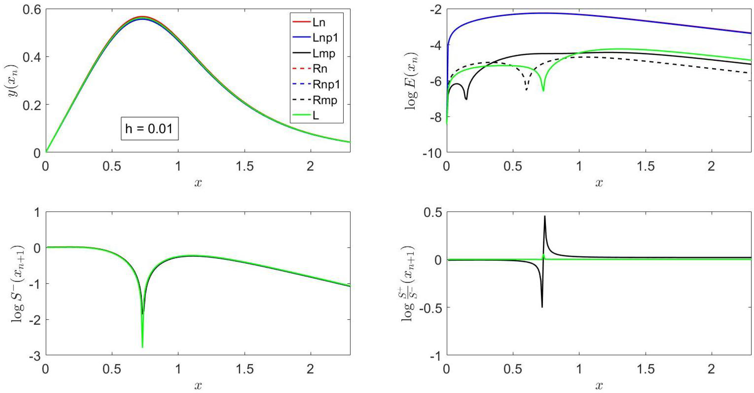
where $C=9-4\sqrt{5}$. This solution tends to zero as $x\to \infty$ and exhibits a relative maximum at $x\approx 0.73$, as shown in Figure 1.

For this example, the radicand defined in Section 2 is $R^2=8$, and, therefore, the finite difference expression for the methods Rn, Rnp1 and Rmp is that of Equation (23), i.e., the ratio of exponential functions.

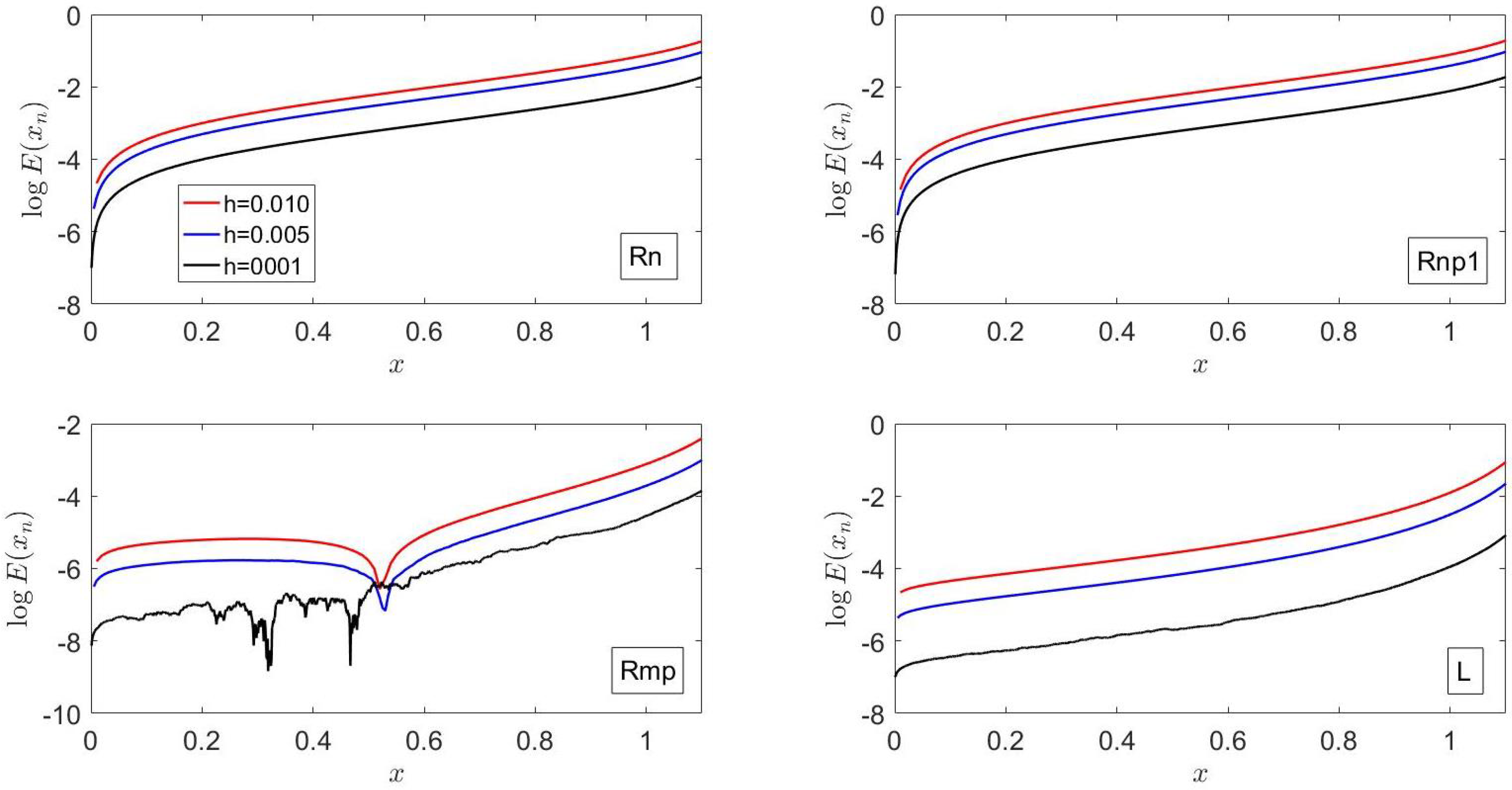
Figure 1 shows that the errors of Ln, Lnp1, Rn and Rnp1 exhibit the same trends and have similar values, which are larger than those of Lmp and Rmp, in accordance with the local truncation error analysis reported in the previous section. The errors of these six methods first increase as x increases from its initial value until $y\left(x\right)$ reaches its relative maximum and then decrease at a smaller rate; i.e., they exhibit the same trends as the analytical solution of Equation (38).

For x greater than unity, Figure 1 indicates that the errors of Lmp and Rmp are smaller than those of L; the error of the latter exhibits a relative minimum at the location of the maximum value of $y\left(x\right)$, i.e., at the location where $f(x,y)=0$.

As shown in Section 2 and Section 3, the piecewise-analytical methods Lmp and Rmp do not account for the dependence of x in $I_n$ since the independent variable is assumed to be equal to $x^{*}$ in that interval; on the other hand, L takes into account that dependence in a linear fashion, as described in Section 3.

Note that, since for $x>>1$, Equation (38) behaves as $y\left(x\right)\approx (2+\sqrt{5})exp(-2x)\equiv V\left(x\right)$, and, therefore, $V\left(x+{\displaystyle \frac{h}{2}}\right)<V\left(x\right)$, one would expect that L is less accurate than Lmp and Rmp for $x>>1$, as illustrated in and in in accordance with the errors shown in Figure 1.

For this example, all the methods presented in this manuscript show that $S_{n+1}^{-}$ decreases from its initial value until $y\left(x\right)$ reaches a relative maximum, then decreases and later increases sharply up to the inflection point of $y\left(x\right)$, exhibits a relative maximum, and then decreases at a much slower rate. The smallest value of the left-side derivative corresponds to L, which includes $f_x$ (cf. Equation (4)).

As illustrated in Figure 1, the ratio of the right- to the left-side derivative is almost one for all $x^n$ except in a neighborhood of the abscissa where the relative maximum of $y\left(x\right)$ occurs; on the left of this abscissa, the slope ratio is less than unity and greater (in absolute value) for Ln, Lnp1, Lmp, Rn, Rnp1 and Rmp than for L, whereas, on the right of this abscissa, the slope ratio is greater than one and greater (in absolute value) for Ln, Lnp1, Lmp, Rn, Rnp1 and Rmp than for L. The behavior of Rn, Rnp1 and Rmp just described is a consequence of the fact that $H^{*}<0$, $|H^{*}|=exp\left(2x^{*}\right)$, increases exponentially as x increases and $J^{*}=2(1-exp\left(2x^{*}\right)y)>0$ for $y<exp(-2x^{*})$, whereas those of Ln, Lnp1, Lmp and L are due to the behavior of $V\left(x\right)$ described above as well as to the fact that $J^{*}<0$ for $y>exp(-2x)$.

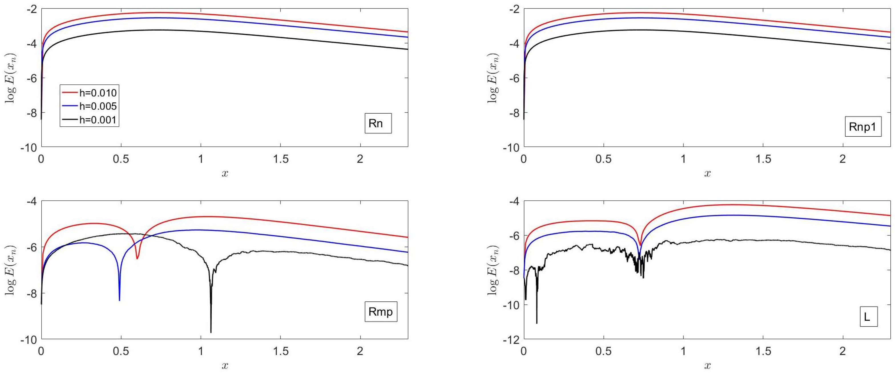
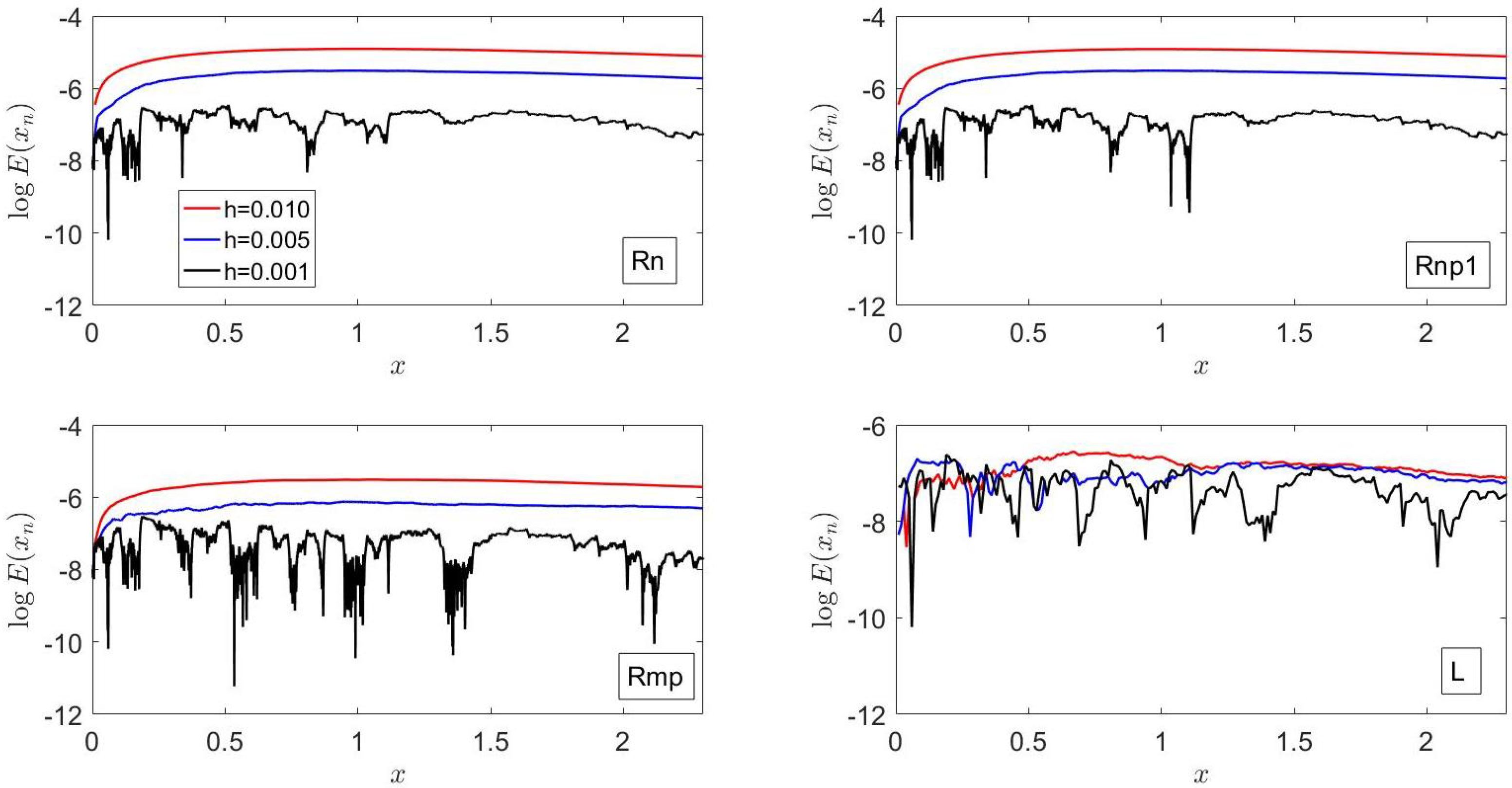
In Figure 2, it is shown that, at $x=1.5$, the accuracy of Rn is about the same as that for Rnp1; the accuracy of these two methods first decreases sharply, reaches a relative minimum, and then increases slowly as x increases; the order of accuracy of these methods is in accordance with what was stated previously in this subsection, as well as with what was is stated in Section 5.

For $h\le 0.005$, Rmp is more accurate than L despite the fact that both are $\mathcal{O}\left(h^2\right)$; the opposite behavior is, however, observed for $h>0.005$. The difference in accuracy between these two methods is mainly due to the coefficient that multiplies the $\mathcal{O}\left(h^3\right)$ term in Equation (32), as discussed in greater length in example 5 below.

6.2. Example 2

This example corresponds to

$${\displaystyle \frac{dy}{dx}}=exp\left(2x\right)+2y+exp(-2x)y^2,x>0,y\left(0\right)=-1,$$

(40)

whose solution is

$$y\left(x\right)=exp\left(2x\right){\displaystyle \frac{tanx-1}{tanx+1}},$$

(41)

and exhibits blowup in finite time at $tanx=-1$, i.e., $x={\displaystyle \frac{3}{4}}\pi$; however, since the principal branch of $tanx$ is $\left(-{\displaystyle \frac{\pi }{2}},{\displaystyle \frac{\pi }{2}}\right)$, the results presented here correspond to this branch.

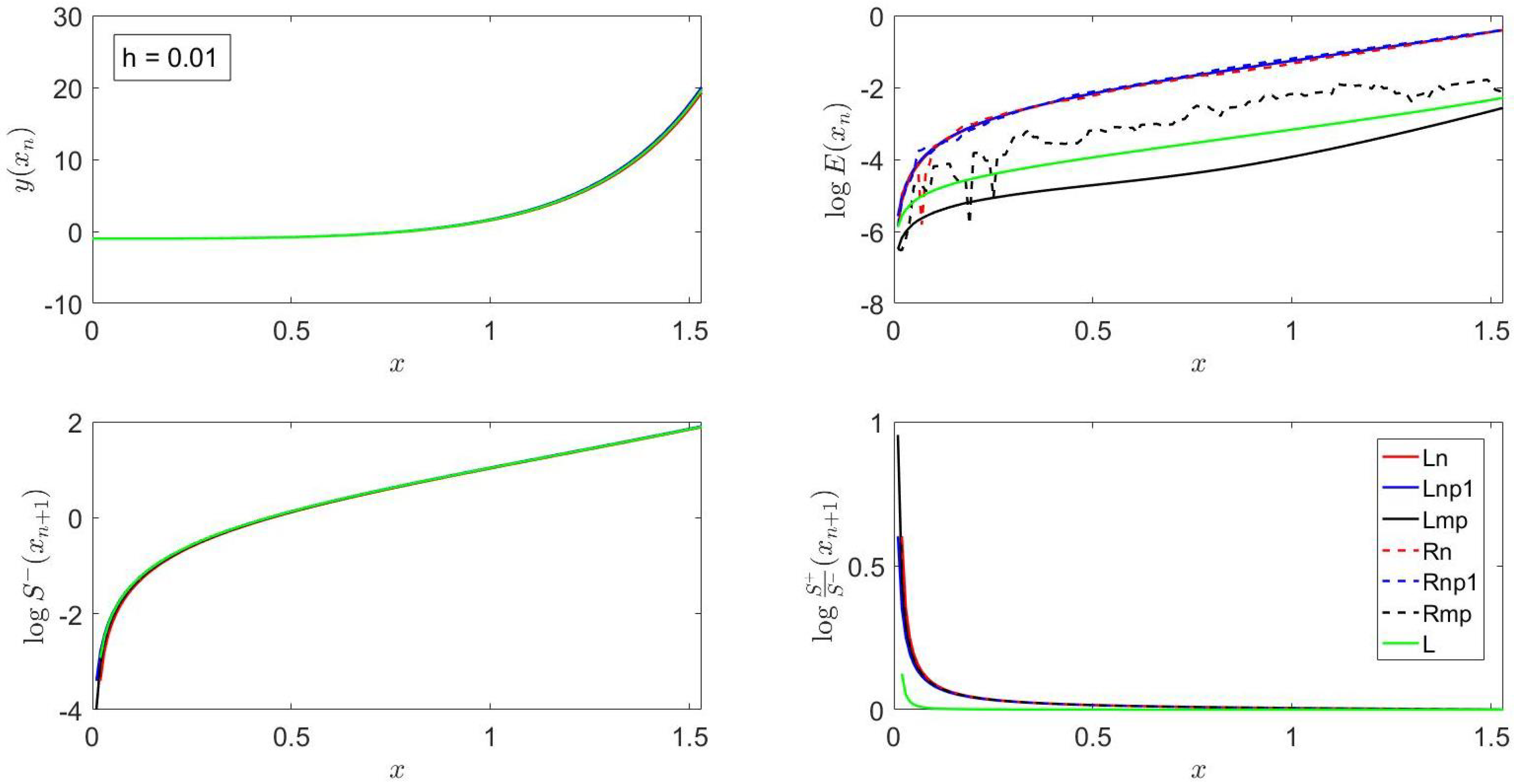
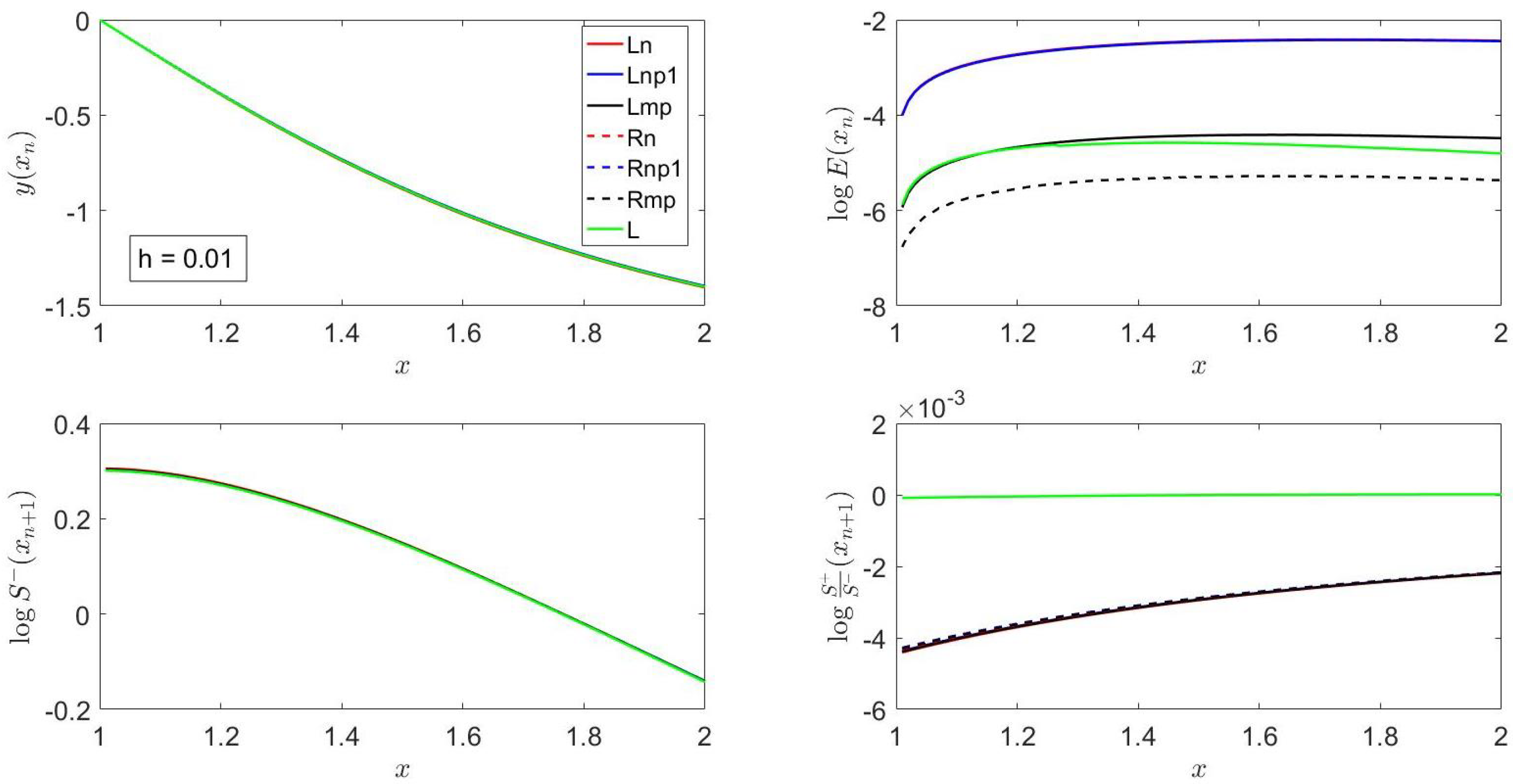
Figure 3 indicates that the exact solution increases as x increases; in fact, for $x\to {\left({\displaystyle \frac{\pi }{2}}\right)}^{-}$, $y\left(x\right)\approx exp\left(2x\right)\equiv V\left(x\right)$. Moreover, for this example, $R=0$ (cf. Section 2), and, therefore, the finite difference equation for the methods Rn, Rnp1 and Rmp is that of Equation (24).

Figure 3 also shows that Lmp is the most accurate method; L is more accurate than Rn; the accuracy of Rmp is lower than that of L but higher than that of Rnp1; and the accuracy of Rnp1 is comparable to those of Ln, Lnp1 and Rn. These results are in accordance with the local truncation error analysis reported in Section 5 and the smooth behavior of Equation (40) in the principal branch of $tanx$.

The errors illustrated in Figure 3 increase as x is increased in accordance with the fact that the exact solution given by Equation (40) increases as x increases. Figure 3 also shows that all the methods presented here provide almost the same value of $S_{n+1}^{-}$ except near $x=0$ due to the exponential dependence of the coefficients that appear in Equation (40). On the other hand, the slope ratio is much larger for Ln, Lnp1, Lmp, Rn, Rnp1 and Rmp than for L due to the fact that the latter makes use of $f_x$ (cf. Equation (4)) and, therefore, accounts for the (explicit) dependence on x in $I_n$ (through $f_x$), as indicated in Section 3.

Figure 3 also shows that Ln, Lnp1, Rn, and Rnp1 exhibit the same trends and have similar errors: these methods are less accurate than Rmp, which, in turn, is less accurate than L, and the latter is, in turn, less accurate than Lmp. The higher accuracy of Lmp as compared with that of L is due to the fact that, since $y\left(x\right)$ is an increasing function of x for $x>>1$, $V\left(x+{\displaystyle \frac{h}{2}}\right)>V\left(x\right)$; in addition, for $x\to {\left({\displaystyle \frac{\pi }{2}}\right)}^{-}$, ${\displaystyle \frac{d^{m+1}V}{d{x}^{m+1}}}=(m+1){\displaystyle \frac{d^{m}V}{d{x}^m}}>V\left(x\right)$ for $m\ge 1$. On the other hand, the lower accuracy of Rmp compared with that of Lmp for this example is due to the fact that, since $R^{*}=0$, $\lambda =-{\displaystyle \frac{J^{*}}{2}}$ (cf. first line below Equation (11)), and $J^{*}=2(1+exp(-2x^{*})y)>0$, $H^{*}=exp(-2x^{*})>0$ and $P^{*}>0$ (cf. Equations (40) and (24)).

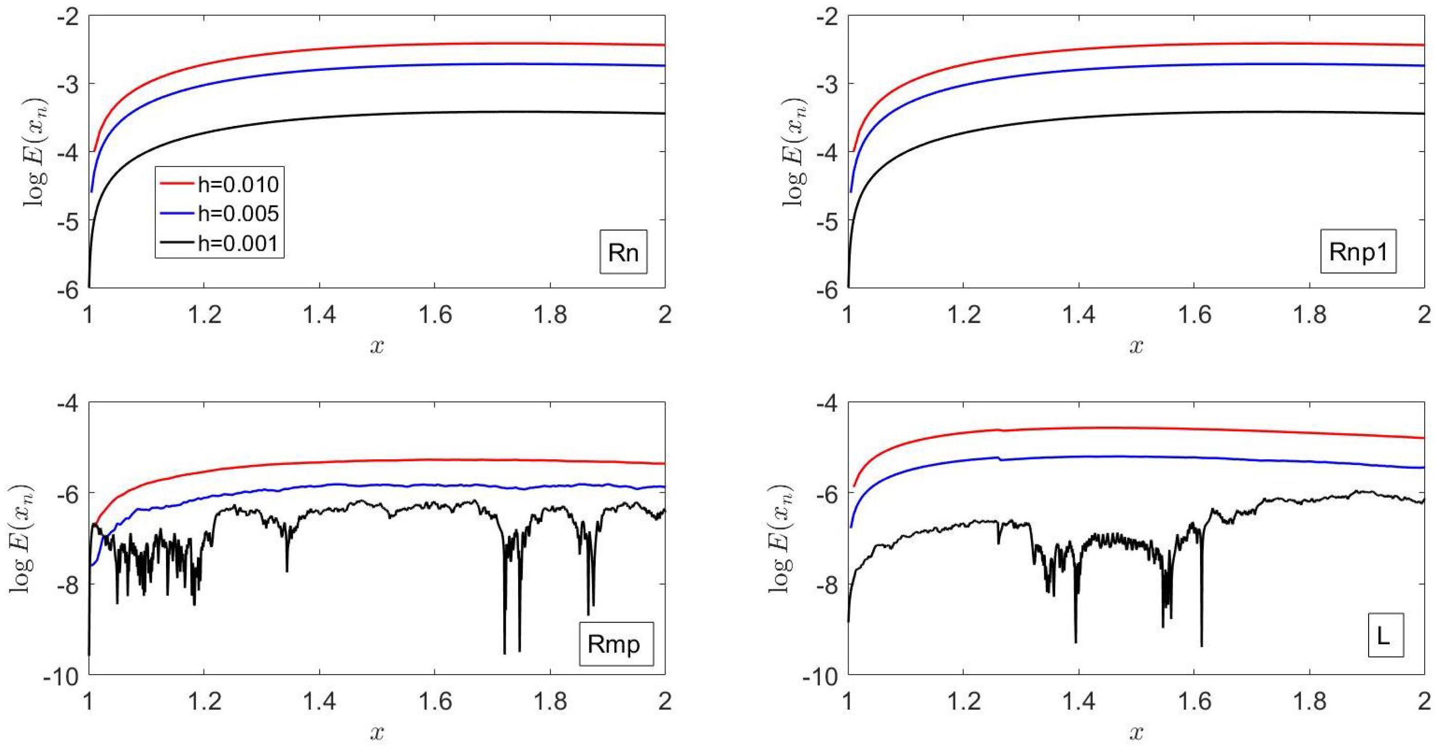
Figure 4 shows that the errors of Rn exhibit similar trends to those of Rnp1, but the errors of these two methods do not exhibit a monotonic behavior with h for all $x>0$. For example, the accuracy of Rnp1 is lower for $h=0.001$ than for $h=0.01$ initially, whereas the opposite behavior is observed at later times. A similar behavior is observed for $h=0.005$. This is in marked contrast with the accuracy of $\mathsf{L}$, which depends monotonically on h, i.e., it increases as h is decreased and is greater than those of Rn, Rnp1 and Rmp; this is consistent with the fact that, as indicated previously, for this example, $R^{*}=0$, but $J\ne 0$ and L depends on $A^n=f_x(x^n,y^n)$, $Q^n=J^n$ and h (cf. Equations (2)–(4)). In addition, L depends exponentially on J and h, whereas Rn, Rnp1 and Rmp depend algebraically on J and h as indicated in Equations (28) and (24), respectively.

On the other hand, the accuracy of Rmp seems to decrease as h is decreased but is higher than those of Rn and Rnp1 for $h\ge 0.005$. The behavior of Rmp on h observed in Figure 4 is due to the exponential coefficients that appear in Equation (40) and the fact that $f>0$, $J>0$ and $H>0$, which imply that, for $x\to {\left({\displaystyle \frac{\pi }{2}}\right)}^{-}$, $f\to 4exp\left(2x\right)$, $J\to 4$ and $H\to exp(-2x)$. This, in turn, implies that Equation (24) may be approximated by $y^{n+1}\approx y^n+4exp\left(2x^n\right){\displaystyle \frac{h}{1+2h}}$, which, for $h<<1$, becomes $y^{n+1}\approx y^n+4exp\left(2x^n\right)h$, which corresponds to Euler’s forward or explicit method.

6.3. Example 3

This example corresponds to

$${\displaystyle \frac{dy}{dx}}=exp\left(x^{4/3}\right)+exp(-x^{4/3})y^2+\left(1+{\displaystyle \frac{4}{3}}{x}^{1/3}\right)y,x>0,y\left(0\right)=0,$$

(42)

whose exact solution is

$$y\left(x\right)=-2exp\left(x^{4/3}\right){\displaystyle \frac{tan\left(\frac{\sqrt{3}}{2}x\right)}{tan\left(\frac{\sqrt{3}}{2}x\right)-\sqrt{3}}},$$

(43)

and exhibits blowup in finite time at $tan\left({\displaystyle \frac{\sqrt{3}}{2}}x\right)-\sqrt{3}=0$, i.e., at $x\approx 1.209$. Note that $y\left(x\right)\approx x$ for $x<<1$ and that the last term in the right-hand side of Equation (42) is not differentiable at $x=0$; however, ${\displaystyle \frac{dy}{dx}}\left(0\right)=1$ and the total derivative of the third term in the right-hand side of Equation (42) with respect to x at $x=0$ is 1. In the neighborhood of the blowup time, $y\left(x\right)\approx -2exp\left(x^{4/3}\right)$.

For this example, $R^2={\displaystyle \frac{16}{9}}\left({\theta }^2+{\displaystyle \frac{3}{2}}\theta -{\displaystyle \frac{27}{16}}\right)$ (cf. Section 2), where $\theta =x^{2/3}$, whose zeroes are $\theta ={\displaystyle \frac{3}{4}}$ and $-{\displaystyle \frac{9}{4}}$, but only the former is a valid one. Moreover, since $\theta \ge 0$, $R^2>0$ for $0\le x\le \varphi \equiv {\left({\displaystyle \frac{3}{4}}\right)}^{{\displaystyle \frac{3}{2}}}$, $R^2=0$ for $x=\varphi$ and $R^2<0$ for $x>\varphi$ and, therefore, these three cases correspond to Equations (25), (24) and (23), respectively. This implies that, as x is increased from zero, the finite difference equations of the Rn, Rnp1 and Rmp methods evolve from the ratio of trigonometric functions to the ratio of exponential ones.

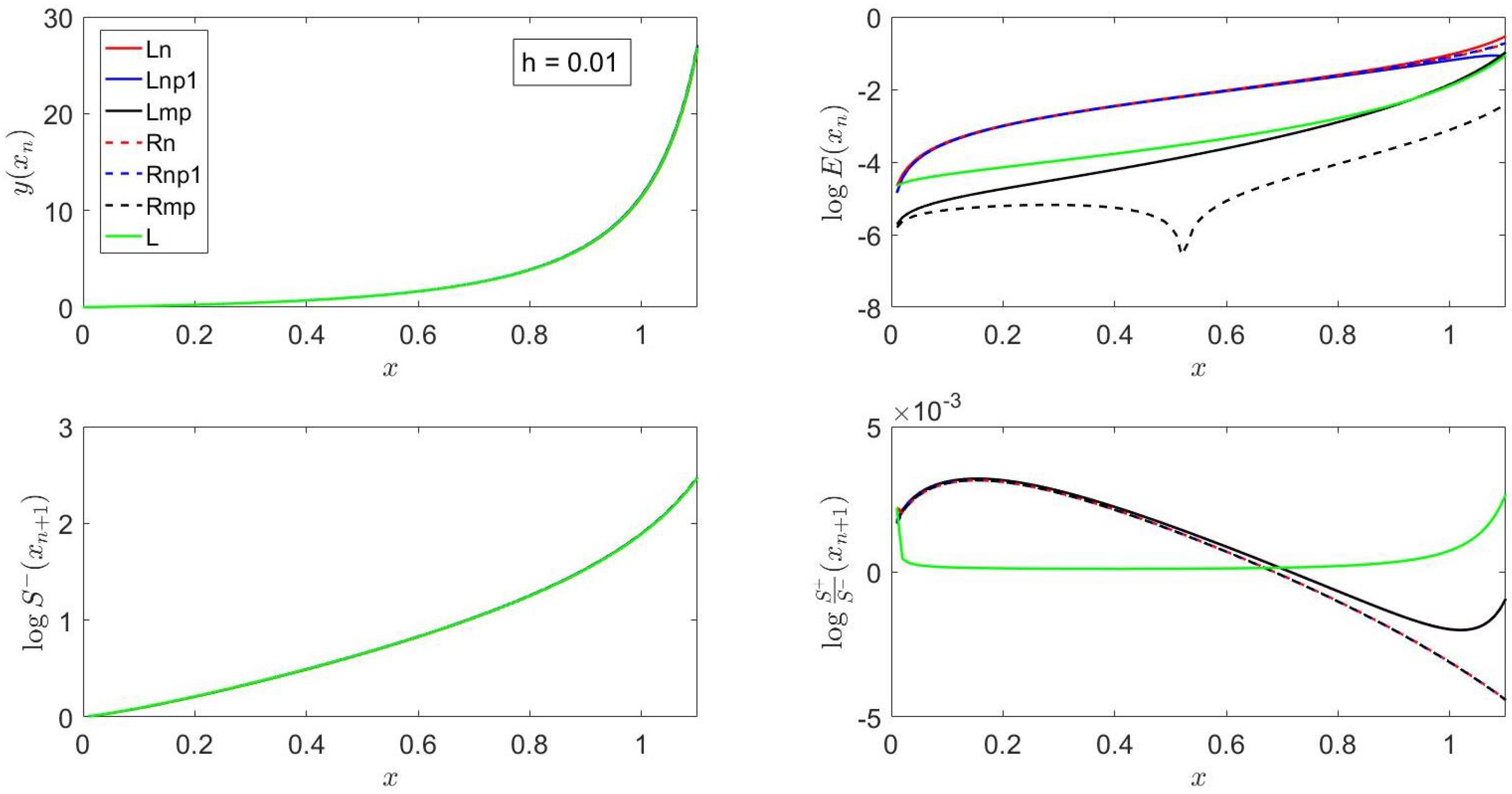
Figure 5 shows that Lmp is more accurate than L, which, in turn, is more accurate than Lnp1; the latter is, in turn, more accurate than Rnp1, whose accuracy is comparable to but higher than that of Ln. These results are consistent with the fact that the coefficients that appear in Equation (42) depend on x, and Ln, Lnp1 and Lmp evaluate these coefficients at different $x^{*}$, whereas, although L makes use of a Taylor series expansion with respect to both the independent and dependent variables, this expansion is a linear one, and its coefficients are evaluated at $x^n$, as shown in Section 2.

Figure 5 also shows that the most accurate method is Rmp and that the slope ratio at $x^{n+1}$ is very close to one for all the methods considered in this manuscript. L predicts the closest slope ratio to unity, followed by Lmp, which exhibits similar trends to those observed by the other methods presented in this paper except near the blowup time. Note that $H=exp(-x^{4/3})>0$, $J=2exp(-x^{4/3})y+1+{\displaystyle \frac{4}{3}}{x}^{1/3}>0$, $f>0$ and Rmp accounts for $P^{*}$, $J^{*}$ and $H^{*}$, whereas Lmp only accounts for $P^{*}$ and $J^{*}$, and L accounts for $P^n$, $J^n$ and $A^n$ (cf. Equations (23)–(31)).

It should be noted that the errors of the numerical methods presented here increase very steeply as the blowup time is approached; this is consistent with the fact that the singularity of the solution derivatives increases as their order is increased. It should also be noticed that an accurate study of blowup in finite time requires the use of variable step sizes whose magnitude decreases as, for example, the slope of the solution increases. This was not pursued in this paper, which is concerned with piecewise-analytical solutions to initial-value problems of nonlinear, first-order, ordinary differential equations. Nevertheless, some comments on the numerical solution of problems that exhibit blow up in finite seem to be appropriate here.

Blowup phenomena in finite time are currently being investigated by the author using variable step sizes based on the slope and/or curvature of the solution; the growth or decay of the solution, etc.; and modifications of the methods L, Lmp and Rmp reported in this manuscript.

Strictly speaking, blowup in either ordinary or evolution partial differential equations means that the solution becomes unbounded at a finite time. When this occurs, the solution loses regularity in a finite time. Since numerical methods cannot deal with infinite values, the issues of how to numerically determine solutions near the blowup time accurately and how to compute an approximate blowup time are of great current interest. Numerical experiments performed to date indicate that adaptive methods can reproduce finite-time blow-up reasonably well; however, they usually do not faithfully reproduce the solution and the blowup rate. In addition, it has been observed that different discretizations result in different growth rates and may introduce spurious behavior in the neighborhood of singularities.

The results presented in Figure 6 indicate that Rn, Rnp1 and L exhibit the same accuracy trends; the accuracy of Rn is comparable to that of Rnp1, which, in turn, is smaller than that of L; and Rmp is more accurate than L. Moreover, close to the blowup time, the errors of L are smaller than those of Rn and Rnp1 but larger than those of Rmp. The higher accuracy of Rmp is due to the fact that this method accounts for $f_{yy}$ (cf. Equation (3)), which, when close to the blowup time, is more singular than $J=f_y$, while the lower accuracy of Rn and Rnp1 is due to the dependence of the coefficients of Equation (42) on x and the fact that $f^{*}$, $J^{*}$ and $H^{*}$ are evaluated at $x^n$ and $x^{n+1}$, respectively.

6.4. Example 4

This example corresponds to

$${\displaystyle \frac{dy}{dx}}=-{\displaystyle \frac{2}{x}}+{\displaystyle \frac{y}{x}}+{\displaystyle \frac{y^2}{x}},x>0,y\left(0\right)=1,$$

(44)

whose solution is

$$y\left(x\right)=2{\displaystyle \frac{1-x^3}{2+x^3}},$$

(45)

and tends to $-2$ as $x\to \infty$ in a monotonic fashion.

For $y\left(0\right)=1$, the finite difference expressions for L, Ln, Rn exhibit a singularity at $x=0$. For this reason, the results presented here correspond to the initial condition $y\left(1\right)=0$ and $x\ge 1$.

For this example $R^2={\displaystyle \frac{9}{x^2}}>0$ (cf. Section 2) and, therefore, the finite difference expressions for the methods Rn, Rnp1 and Rmp are those corresponding to Equation (23). Moreover, $J={\displaystyle \frac{1}{x}}(1+2y)$ and $H={\displaystyle \frac{1}{x}}$. This means that f, R, J, H tend to zero as $x\to \infty$ and, therefore, the finite difference Equation (23) tends to that of Equation (24) as $x\to \infty$.

Figure 7 indicates that, for $x\gtrsim 1.3$, L is more accurate than Lmp, which, in turn, is more accurate than Ln, Lnp1, Rn and Rnp1; the latter four methods do not only exhibit similar trends they also have similar accuracy. The results presented in Figure 7 are in accordance with the local truncation error analysis reported in Section 5. The differences between the errors of L and Lmp, which are both second-order accurate, are mainly due to the coefficient that multiplies the $\mathcal{O}\left(h^3\right)$ in Equation (32) which includes second- and higher-order derivatives of $f(x,y)$.

Figure 7 also indicates that the most accurate method is Rmp for $h=0.01$; L predicts the closest slope ratio to unity; and Ln, Lnp1, Rn, Rnp1 and Rmp predict analogous slope ratios.

Figure 8 indicates that the accuracy of Rn is comparable to that of Rnp1 and both methods exhibit the same trends; the accuracy of Rn is lower than that of L whose accuracy, in turn, is smaller than that of Rmp for $h\ge 0.005$; and the accuracy of all the methods presented in this figure first decreases, then reaches a relative maximum and then increases at a slow pace except for L and Rmp for $h=0.001$.

6.5. Example 5

This example corresponds to

$${\displaystyle \frac{dy}{dx}}=-exp\left(x\right)y^2+y-exp(-x),x>0,y\left(0\right)=1,$$

(46)

whose solution is

$$y\left(x\right)=exp(-x),$$

(47)

and decreases exponentially as x increases.

For this example, $R^2=-3$ and, therefore, the finite difference equation for the methods Rn, Rnp1 and Rmp is Equation (25). This means that the explicit finite difference Equations (23)–(25) are the ratios of trigonometric functions, whereas those of L, Ln, Lnp1 and Lmp are of exponential type because they depend exponentially on $Jh$ (cf. Equations (28) and (30)). Moreover, $f>0$, $H<0$, and $J<0$. Note also that $\left|H\right|\to \infty$ as $x\to \infty$ in an exponential fashion.

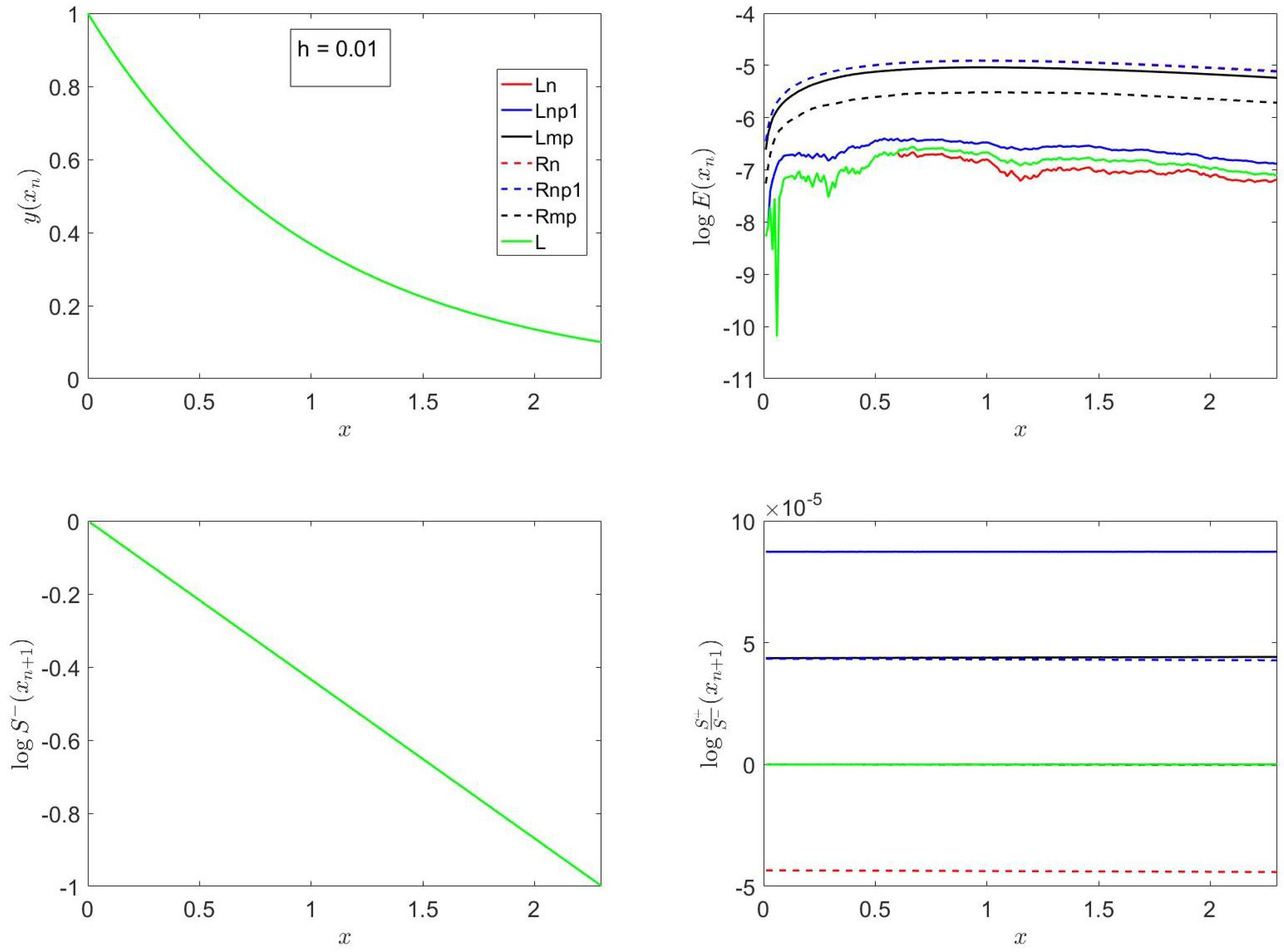
Figure 9 indicates that the most accurate method for this example is Ln, followed by L, Lnp1, Rmp, Lmp, Rn and Rnp1. This result is due to the fact that the exact solution decreases exponentially with time, the time-dependent coefficients that appear in Equation (46) are exponential functions of time, $J<0$, and $\left|H\right|$ increases exponentially with time, as stated above. In addition, Ln and Lnp1 evaluate their corresponding first-order Taylor series approximation at $x^n$ and $x^{n+1}$, respectively, as indicated in Section 3 and, therefore, $exp\left(x^n\right)>exp\left(x^{n+1}\right)$.

Figure 9 also shows that the differences between the errors of Ln and L are very small; in fact, the errors of these two methods are almost identical for $x\lesssim 0.66$. In addition, the slope ratio predicted by all the methods presented in this paper is very close to unity, as illustrated in Figure 9, although Rn predicts a slope ratio slightly less than one, whereas Ln, Lnp1, Lmp, Rmp and Rnp1 predict a slope ratio slightly greater than unity for $h=0.01$.

The results illustrated in Figure 10 show that the errors of Rn are comparable to those of Rnp1 and decrease as h is decreased; these errors are larger than those of L, which, in turn, are smaller than those of Rmp, except for $h=0.001$. The reason for this behavior has been explained above; i.e., for $H^{*}\ne 0$, the approximate, piecewise-analytical methods Rn, Rnp1 and Rmp involve the ratio of trigonometric functions, whereas the linear methods Ln, Lnp1, Lmp and L are of the exponential type. Note also that for non-autonomous, nonlinear, ordinary differential equations, L is second-order accurate, as indicated in Section 5.

The results presented in Figure 1, Figure 2, Figure 3, Figure 4, Figure 5, Figure 6, Figure 7, Figure 8, Figure 9 and Figure 10 clearly indicate that the most accurate method for Examples 1, 3 and 4 is Rmp for $h=0.01$. These three examples are characterized by well-behaved solutions that first increase and then decrease with x for example 1 and solutions that exponentially growi or decrease for examples 3 and 4, respectively. However, the accuracy of this method decreases substantially for equations with solutions that blow up in finite time, as in example 2 and equations with $R^2<0$ (cf. Section 2) with exponentially decaying solutions; the loss of accuracy in these cases is due to exponentially growing second-order derivative $f_{yy}$ and the ratio of trigonometric functions (cf. Equation (25)), respectively.

6.6. Accuracy of the Linear and Quadratic Approximations Methods at Selected Times

In this subsection, the accuracy of the linear approximation methods L, Ln, Lnp1 and Lmp, as well as that of the quadratic ones Rn, Rnp1 and Rmp, is presented for the five examples considered in previous subsections at selected times.

In

Table 1. Decimal logarithm of the error $E\left(x\right)$, i.e., $logE\left(x\right)$, at selected times.

Example ($\mathit{x}=1.5$)	h	Ln	Lnp1	Lmp	L	Rn	Rnp1	Rmp
1	0.010	−2.68	−2.69	−4.51	−4.29	−2.68	−2.69	−4.93
1	0.005	−2.98	−2.99	−5.12	−4.90	−2.98	−2.99	−5.56
1	0.001	−3.68	−3.69	−6.36	−6.30	−3.68	−3.69	−6.22
Example ($x=1.5$)	h	Ln	Lnp1	Lmp	L	Rn	Rnp1	Rmp
2	0.010	−0.46	−0.45	−2.65	−2.35	−0.46	−0.45	−1.88
2	0.005	−0.76	−0.76	−3.25	−2.95	−0.56	−1.13	−1.64
2	0.001	−1.46	−1.49	−4.55	−4.47	−0.85	−0.67	−0.47
Example ($x=1.0$)	h	Ln	Lnp1	Lmp	L	Rn	Rnp1	Rmp
3	0.010	−1.00	−1.20	−1.86	−1.90	−1.12	−1.11	−3.11
3	0.005	−1.39	−1.46	−2.45	−2.51	−1.42	−1.41	−3.71
3	0.001	−2.11	−2.12	−3.89	−3.95	−2.12	−2.11	−4.54
Example ($x=2.0$)	h	Ln	Lnp1	Lmp	L	Rn	Rnp1	Rmp
4	0.010	−2.44	−2.45	−4.48	−4.80	−2.44	−2.44	−5.37
4	0.005	−2.74	−2.75	−5.09	−5.46	−2.75	−2.75	−5.89
4	0.001	−3.44	−3.44	−6.48	−6.12	−3.44	−3.45	−6.35
Example ($x=1.5$)	h	Ln	Lnp1	Lmp	L	Rn	Rnp1	Rmp
5	0.010	−7.02	−6.56	−5.08	−6.81	−4.95	−4.95	−5.54
5	0.005	−6.90	−6.90	−5.68	−6.90	−5.56	−5.56	−6.20
5	0.001	−7.17	−7.17	−7.67	−7.17	−6.73	−6.73	−7.17

, the decimal logarithm of the error, i.e., $logE\left(x\right)$, at selected times is presented for all the methods and the five examples considered in this paper. This table shows that the errors decrease as the step size is decreased except for Rnp1 and Rmp for example 2; Lmp is more accurate than Ln and Lnp1 for all the examples, except for example 5 and $h\ge 0.005$; L is more accurate than Lmp for example 2 and examples 4 and 5 for $h\ge 0.005$; and Rmp is more accurate than Rn and Rnp1 for examples 1, 3, 4 and 5 and example 2 for $h\le 0.005$.

Table 1 also indicates that, for $h=0.01$, the most accurate method is Lmp for examples 1 and 2, and L, Rmp and Ln are the most accurate methods for examples 3, 4 and 5, respectively. Table 1 also shows that L exhibits an order of convergence slightly above two for examples 1, 2, 3 and 5 and between 1 and 2 for example 4. On the other hand, the order of convergence of Lmp is greater than two for examples 3 and 5, two for example 4, and slightly below two for examples 1 and 2. These orders of convergence are mainly in accordance with the local truncation errors analysis reported in Section 5, which are based on Taylor series expansions of the finite difference equations and require that the step size be small. But even though, for example, L and Rmp are second-order accurate methods (cf., e.g., Equation (32)), the coefficient of the $\mathcal{O}\left(h^3\right)$ term in that equation, which is proportional to the second- and higher-order derivatives of $f(x,y)$, may become so large that the neglected $\mathcal{O}\left(h^3\right)$ term may become comparable to or even larger than (the lower-order) retained ones. This may be the case for problems that exhibit blowup in finite time, such as example 3, and problems with very fast-growing or decaying solutions, such as examples 1, and 2 and 5, unless h is sufficiently small. When such a problem is observed, the step size should be varied according to the solution behavior.

For the five examples considered in this section, except example 2, the accuracy of Rn is very close to that of Rnp1, and the accuracy of Ln is very close to that of Lnp1 for examples 1, 2 and 4 and example 5 with $h\le 0.005$, but lower than that of Lnp1 for example 3.

Note that the comments made above on the results in Table 1 are only valid for the times specified in that table and, therefore, may not be applicable to the whole range of x considered in the examples illustrated in Figure 1, Figure 2, Figure 3, Figure 4, Figure 5, Figure 6, Figure 7, Figure 8, Figure 9 and Figure 10 of this paper.

6.7. Comparisons with Other Numerical Procedures

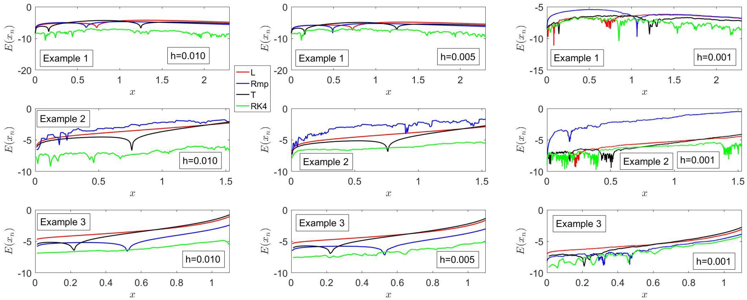
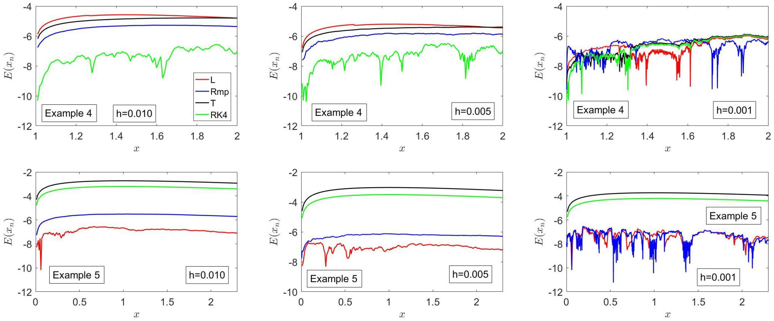
In this subsection, comparisons between the results of the second-order accurate L and Rmp methods presented in this paper and those of the second-order trapezoidal scheme (T), and the fourth-order Runge–Kutta technique (RK4) are presented for the five examples considered in the manuscript. Such comparisons are made in terms of the error with respect to the exact solution and for three different step sizes and are illustrated in Figure 11 and Figure 12.

Before discussing these figures, it is convenient to emphasize several points. First, L and Rmp are implicit methods that provide explicit finite difference formulae, as indicated in Section 5; T is an implicit scheme that, for the nonlinear ordinary differential equations of examples 1–5, result in nonlinear algebraic equations that were solved iteratively by means of the Newton–Raphson technique with the convergence criteria: $E_k=|y_{k+1}-y_k|\le h^2$ and $R_k={\displaystyle \frac{E_k}{|y_{k+1}|}}\le h^2$ provided that $y_{k+1}\ne 0$, where the subscript k denotes the k-th iteration within each $[t^n,t^{n+1}]$, and RK4 is a four-stage, explicit scheme. Second, L and Rmp are $A_0$-stable; T is A- but not $A_0$-stable; and RK4 is conditionally stable. Third, although L, Rmp and T are second-order accurate, the coefficient that multiplies the $\mathcal{O}\left(h^3\right)$ term in Equation (32) is different for each of these methods; this should be kept in mind when comparing the errors of these methods, as indicated previously in the subsection on example 5. Fourth, for the examples whose solutions exhibit either blowup in finite time or grow exponentially, the use of a fixed step size in the trapezoidal rule usually results in an increase in the number of iterations required for convergence, i.e., an increase in the computational time, and not very accurate solutions if the step size is not sufficiently small; however, only the accuracy of L and Rmp is affected in such cases. Fifth, for the same step size, RK4 requires more operations than T, and, for the examples and time steps considered in this work, T required more operations (due to its iterative character) than Rmp, which, in turn, required a few more operations than L. And, sixth, Rmp makes use of $f(x,y)$ and its first- and second-order derivatives with respect to the dependent variable, and L makes use of $f(x,y)$ and its first-order derivative with respect to the dependent variable, whereas T and RK4 only make use of $f(x,y)$. This means that step adaptation comes in a natural way for both L and Rmp through the magnitude of $f_y$, whereas that of T would require, for example, computations based on different step sizes as discussed at the beginning of this section. RK4 could also be used as an adaptive strategy based on computations with different step sizes as just described for T or embedded formulations such as, for example, the Runge–Kutta–Fehlberg–45 procedure.

Figure 11 shows that for $h\le 0.005$ and example 1, the methods considered in this section can be ordered in terms of accuracy (from higher to lower) as RK4, T, Rmp and L, but the errors of the latter three are similar. However, for $h>0.005$, the ordering is RK4, T, L and Rmp for $x\lesssim 1.25$ and RK4, T, Rmp and L for $x>1.25$.

For Examples 2 and 3, the ordering of accuracy is RK4, T, Rmp and L, and RK4, Rmp, T and L, respectively. As stated previously, the solution to example 2 is an exponentially growing one, whereas that of example 3 exhibits blowup in finite time.

Figure 12 shows that the accuracy order for example 4 is RK4, Rmp, T and L, for $h\le 0.005$, and Rmp, L, T and RK4, for $h>0.005$. By way of contrast, the accuracy ordering for example 5 is L, Rmp, RK4 and T, for $h\le 0.005$, and Rmp, L, RK4 and T, for $h>0.005$. Note that, as stated previously, the solution to example 5 is an exponentially decreasing one and that Rmp and L make use of $f_y$ and $f_{yy}$, and $f_y$, respectively.

The results presented in Figure 11 and Figure 12 clearly illustrate that although L, Rmp and T are second-order accurate and their errors are $\mathcal{O}\left(h^2\right)$, the magnitude of their errors may be different due to the difference in the coefficient that multiplies the $\mathcal{O}\left(h^3\right)$ term in their series expansions (cf. Equation (32)).

For example 5, the results illustrated in Figure 12 indicate that L, Rmp are more accurate than T and RK4 because L and Rmp account for f and $f_y$; Rmp also accounts for $f_{yy}$, whose absolute value is an exponentially increasing function of time. On the other hand, T and RK4 only account for f, as discussed previously.

7. Conclusions

Approximate piecewise-analytical solutions to scalar, nonlinear, first-order, ordinary differential equations have been reported based on fixing the independent variable on the right-hand side of these equations and approximating the resulting term by either its first- or second-order Taylor series expansion.

For second-order Taylor series truncations, the approximate methods presented here result in Riccati equations with constant coefficients whose analytical solutions are obtained as the ratio of polynomials, trigonometric or exponential functions instead of the ratio of the two series that result when the Taylor series expansions also include the dependence on the independent variable.

For first-order Taylor series approximations, the piecewise-analytical methods presented here result in first-order, linear, ordinary differential equations with constant coefficients and result in exponential solutions, whereas the solution of linearized methods based on first-order Taylor series approximations that also account for the dependence on the independent variables include exponential and first-degree polynomials.

The approximate piecewise-analytical methods based on both the first- and the second-order Taylor’s series approximations of the right-hand side of the ordinary differential equations have been shown to result in explicit finite difference methods that are unconditionally stable.

Numerical experiments carried out on five first-order, nonlinear, ordinary differential equations that have analytical solutions that either grow or decrease monotonously, first increase and then decrease, or exhibit blowup in finite time have been performed in order to assess the accuracy of the methods presented in the paper. For three of these equations, which exhibit either monotonically decreasing or increasing solutions or solutions that first increase and then decrease, it has been found that a second-order Taylor series expansion of the right-hand side of the differential equation evaluated at each interval’s midpoint results in the most accurate method, whereas methods based on either first- or second-order Taylor series expansion of the right-hand side of the differential equation evaluated at the left and right points of each interval have similar accuracy, except for the second example considered in this study.

For one example that exhibits blowup in finite time, it has been found that methods based on a second-order Taylor series expansion may result in very much poorer accuracy than those based on a first-order expansion, as the blowup time is approached due to the increase in the singularity of the derivatives with respect to the dependent variable as their order is increased. However, the accuracy of first- and second-order Taylor series expansion methods for blowup problems may be substantially improved by employing variable step sizes that are changed according to, for example, the slope of the solution.

It has also been found that if the radicand of a quadratic equation that depends on the right-hand side of the nonlinear, ordinary differential equations and its first- and second-order derivatives is negative, the accuracy of the quadratic approximation methods presented in this manuscript is much smaller than those based on linear approximations because the former are characterized by finite difference expressions that are the ratio of trigonometric functions, whereas the latter depend exponentially on the first-order partial derivative of the right-hand side with respect to the dependent variable.

It has also been shown that the accuracy of the methods Rmp and L presented in this paper is of the same order as that of a trapezoidal rule that requires an iterative procedure, whereas Rmp and L provide explicit finite difference formulae that are $A_0$-stable.