Q-Learning for Online PID Controller Tuning in Continuous Dynamic Systems: An Interpretable Framework for Exploring Multi-Agent Systems

Abstract

This study proposes a discrete multi-agent Q-learning framework for the online tuning of PID controllers in continuous dynamic systems with limited observability. The approach treats the adjustment of each PID gain ($k_p$, $k_i$, $k_d$) as an independent learning process, in which each agent operates within a discrete state space corresponding to its own gain and selects actions from a tripartite space (decrease, maintain, or increase its gain). The agents act simultaneously under fixed decision intervals, favoring their convergence by preserving quasi-stationary conditions of the perceived environment, while a shared cumulative global reward, composed of system parameters, time and control action penalties, and stability incentives, guides coordinated exploration toward control objectives. Implemented in Python, the framework was validated in two nonlinear control problems: a water-tank and inverted pendulum (cart-pole) systems. The agents achieved their initial convergence after approximately 300 and 500 episodes, respectively, with overall success rates of $49.6\%$ and $46.2\%$ in 5000 training episodes. The learning process exhibited sustained convergence toward effective PID configurations capable of stabilizing both systems without explicit dynamic models. These findings confirm the feasibility of the proposed low-complexity discrete reinforcement learning approach for online adaptive PID tuning, achieving interpretable and reproducible control policies and providing a new basis for future hybrid schemes that unite classical control theory and reinforcement learning agents.

1. Introduction

The Proportional–Integral–Derivative (PID) controller represents the most widely implemented control scheme in industrial systems, characterized by its simple structure, direct physical interpretation, and effectiveness in a wide variety of dynamic processes [1]. Its formulation, based on the combination of proportional, integral, and derivative actions, provides a balanced trade-off between response speed, steady-state error elimination, and oscillation damping, and, in turn, lower implementation costs compared to other robust control techniques, such as dead-time compensation (DTC) or model predictive control (MPC), which explains its widespread adoption in sectors such as manufacturing, chemical industry, robotics, and energy [2,3]. However, the effectiveness of PID critically depends on the proper selection of its gains ($k_p$, $k_i$, $k_d$), which determines the system’s stability and transient performance of the system [2,4]. Inappropriate configuration of these parameters leads to degraded behavior, such as excessive overshoot, persistent oscillations, or slow settling, which in turn result in energy inefficiencies, increased mechanical wear, and productivity losses [1,5]. Furthermore, the adjustment process remains highly dependent on operator experience and the operating environment, resulting in highly variable results and a lack of reproducibility across implementations [4]. This set of factors makes PID tuning one of the main bottlenecks in the performance of industrial control systems, particularly in contexts involving non-stationary or nonlinear behavior [5]. Consequently, understanding the structural advantages and limitations of PID has been essential for the development of adaptive approaches and more generalizable optimization strategies.

In response to the limitations of conventional adjustment methods, there has been sustained development of optimization strategies based on metaheuristic algorithms, designed to address the nonlinear, uncertain, and multivariable nature of industrial processes. These strategies, inspired by biological, physical, or social principles, employ global search mechanisms to estimate the optimal parameters of the PID controller in the absence of accurate models [6,7]. This category includes evolutionary algorithms, such as Genetic Algorithm (GA) and Differential Evolution (DE); swarm algorithms, such as Particle Swarm Optimization (PSO) [7,8].

The attractiveness of these methods lies in their ability to explore complex search spaces without requiring precise knowledge about the process model, offering robust solutions in the face of uncertainty, noise, or parametric variability. In addition, their stochastic nature allows them to avoid local minima, achieving superior results in systems with nonlinear dynamics or significant delays [6]. However, their performance depends heavily on the appropriate parameterization of the algorithm and the definition of the optimization criterion, factors that affect the stability and reproducibility of the results [7]. These challenges, together with their high computational cost, have driven the search for approaches with greater adaptive capacity and less dependence on external calibrations, particularly those based on machine learning techniques, which have gained increasing attention in a wide range of areas of study, including those aimed at evaluating their integration into tuning strategies.

Advances in artificial intelligence algorithms have led to the incorporation of machine learning (ML) techniques in control problems, either directly or through controller tuning, the latter motivated by the need to overcome the limitations of traditional heuristic strategies. These approaches enable the direct extraction of knowledge from process data, modeling nonlinear behaviors and temporal dependencies without the need for a detailed physical model of the system [6,9]. Within the field of ML, three main paradigms are commonly distinguished: supervised learning, used in system identification and modeling tasks; unsupervised learning, aimed at discovering hidden patterns in the data; and reinforcement learning (RL), which has gained relevance due to its ability to autonomously adjust control policies through direct interaction with the environment [10,11,12].

Numerous algorithmic proposals have been developed, including the use of recurrent neural networks (RNNs) and their extensions, such as LSTM, which have proven highly effective in capturing the temporal dynamics of industrial processes, facilitating the development of predictive and adaptive models that generalize better under disturbances and nonlinearities [9]. In turn, deep reinforcement learning architectures, particularly those based on Actor-Critic (AC) structures, and policy-optimization approaches such as Deep Deterministic Policy Gradient (DDPG) and Proximal Policy Optimization (PPO), have enabled the implementation of self-tuning PID controllers capable of optimizing their gains online from reward signals without relying on exact process models [12,13,14,15]. However, the computational cost and the difficulties inherent in hyperparameter selection associated with training limit their large-scale adoption [16,17].

In this context, it is pertinent to investigate the design of hybrid algorithms that combine the robustness and simplicity of PID with the adaptive capacity of more advanced optimization methods. This challenge raises a logical question: Is it possible to design reinforcement learning architectures that maintain transparency and remain effective in continuous control tasks?

One promising approach is to restrict the complexity of the agent and shift the design toward schemes where adaptation mechanisms are observable and interpretable. This involves prioritizing direct interpretability over post-hoc explanations (external methods that seek to explain a black box), allowing for the inspection, verification, and traceability of decisions. In this sense, the study of RL approaches with discretized states and actions, explicit update rules, and low-complexity value/policy functions, such as classic Q-learning or other algorithms that offer an adequate compromise between adaptability and readability of the decision mechanism, are relevant to validate and extend [18]. This is because when these decisions are explicitly set, the perception-decision-action cycle becomes auditable, allowing informed human orchestration or intervention to enhance learning stability [18,19,20], a decisive step toward intelligent control that is verifiable and aligned with industrial requirements for robustness and explainability.

In turn, the evolution toward systems with multiple interconnected agents/controllers has given rise to a set of distributed strategies that combine local autonomy with global cooperation, and highlighting key aspects and promising alternatives for their integration. Among these, studies have shown that exposing consensus relationships among control inputs facilitates the analysis of collective behavior [21]. Asynchronous distributed predictive approaches provide an effective solution in environments where agents operate with heterogeneous sampling times, ensuring stability and compliance with physical constraints even under external disturbances [22]. Meanwhile, studies in distributed differential games have demonstrated that formulating control as a strategic interaction between agents with individual objectives allows Nash equilibria to be achieved through linear feedback laws that consider the partial knowledge of each subsystem [23].

Taken together, these underscore key considerations for incorporating of structural interpretability principles into RL architectures, where coordination and local decisions can be analyzed in terms of their physical impacts and contribution to the overall objective of the system. From this perspective, tabular Q-learning is revisited here as a fundamental strategy for online PID tuning. The central idea is to address the design of an appropriate training framework to analyze how agents progressively configure tuning policies for each PID gain, so that the tuning of each gain can be understood as a sequential decision process evaluated across defined intervals. This approach shifts the focus from mere parameterization of the algorithm to observing how the adjustment itself unfolds over evaluation time windows, highlighting the interaction between reward design, convergence behavior, and the emergence of stabilizing strategies under conditions of reduced observability as well as the lack of access to explicit system models.

To further expand this understanding and address the rapid growth of Q-learning tables, the study adopts a configuration of independent multi-agents, each of which autonomously regulates its own PID gains ($k_p$, $k_i$, $k_d$). Decoupling the search process reduces the complexity of local convergence, favoring scalability toward multi-agent architectures and the design of more robust and transparent strategies for application in industrial environments. However, it also introduces specific challenges, such as the need for implicit coordination, the non-stationarity of the learning environment caused by simultaneous interactions with the environment, and the inherent trade-off that arises between exploration and stability [24]. Given these challenges, this study hypothesizes that a set of independent agents acting within a discrete and limited action space (decrease, maintain, or increase each gain), guided solely by an aggregate global reward function, can effectively explore the parameter space and converge toward stabilizing policies without resorting to complex RL structures. Therefore, the overall objective of this study is to evaluate the feasibility and mechanisms by which this discrete multi-agent Q architecture operates for online PID tuning of continuous dynamic systems.

This objective is detailed through three specific aims:

1.

To determine whether agents with restricted observability in the state space, whose only interaction with the environment is the modification of their own gains, can achieve stabilizing policies from global reward signals.

2.

To analyze the emerging exploration trajectories in the PID parameter space, identifying characteristic patterns of learning and adaptation.

3.

To examine the convergence properties of the learning dynamics, ensuring that the adaptation of the gains results in stable and consistent control behavior.

Rather than competing with deep RL schemes or other tuning algorithms with respect to efficiency or accuracy, the study seeks to provide a deeper understanding of the principles that enable effective integration between two classical approaches: control theory and reinforcement learning. To this end, the paper integrates two consolidated theoretical frameworks: on the one hand, the principles of classical control embodied by PID, particularly those related to the stability and dynamic response of closed-loop systems; and on the other hand, the fundamentals of reinforcement learning, centered on the formalism of Markov decision processes and the convergence properties of the Q-learning algorithm. Both domains exhibit a strong theoretical and operational compatibility, while PID control adjusts system actions in response to error dynamics, reinforcement learning provides a powerful framework for optimizing adaptive decision sequences. This synergy enables the development of simple, interpretable, and scalable architectures, suitable for implementation in resource-constrained industrial environments.

2. Theoretical Frameworks

2.1. Proportional–Integral–Derivative Controller

The PID controller is a closed-loop feedback control mechanism that forms the basis of many industrial automation, robotics and embedded control systems, thanks to its simple formulation and proven effectiveness [2]. In this work, the PID controller is used in its parallel discrete form, expressed as Equation (1), where $u\left(t\right)$ represents to the control signal applied to the system, $e\left(t\right)$ is the error at instant t (defined as $e\left(t\right)=r\left(t\right)-y\left(t\right)$, where $r\left(t\right)$ is the reference signal and $y\left(t\right)$ is the system output), and $k_p$, $k_i$ and $k_d$ are the proportional, integral and derivative gains, respectively. Each term contributes distinctly to system dynamics: the proportional component introduces an immediate correction based on the current error, but if $k_p$ is excessive, it can induce oscillations or instability; the integral component accumulates the error history to eliminate steady-state errors, although it can generate overshoot and the integral wind-up phenomenon if not properly regulated; and the derivative term anticipates the error dynamics, generating a useful damping action to reduce overshoot, although it is sensitive to high-frequency noise in the measured signal. Overall, the PID controller seeks to modulate the system response as a function of temporal error, although the nonlinear interaction among the terms makes tuning a complex and delicate process.

$$u\left[t\right]=k_{p}e\left[t\right]+k_i\sum _{j=0}^{t}e\left[j\right]dt+k_d{\displaystyle \frac{e\left[t\right]-e[t-1]}{dt}}$$

(1)

PID tuning involves identifying an appropriate combination of $k_p$, $k_i$ and $k_d$ values that optimizes system performance according to metrics such as settling time, overshoot, stability, and robustness to perturbations. Historically, empirical methods such as the Ziegler-Nichols [25] (first published in 1942) and Cohen-Coon [26] (first published in 1953) rules have been proposed, useful in first-order linear processes but with limitations in delayed or nonlinear systems. More advanced techniques, such as $lambda$-tuning or IMC-based PID tuning [27], offer a systematic approach that rely on model-based information, with good results in stationary systems. In more complex contexts, methods such as relay feedback [28], adaptive self-tuning algorithms, and heuristic approaches based on optimization (genetic algorithms, Particle Swarm Optimization, Bayesian strategies) have been employed. In addition, approaches have emerged that integrate machine learning and neural networks to determine optimal configurations in complex search spaces. Although these methods have extended the capabilities of PID, in many cases they involve high computational costs or significant dependence on accurate models, which restricts their applicability in dynamic industrial environments. These limitations have motivated the search for alternative methods that allow the PID parameters to be adapted online without requiring an explicit model of the system, a context in which reinforcement learning is positioned as a particularly promising approach.

2.2. Reinforcement Learning

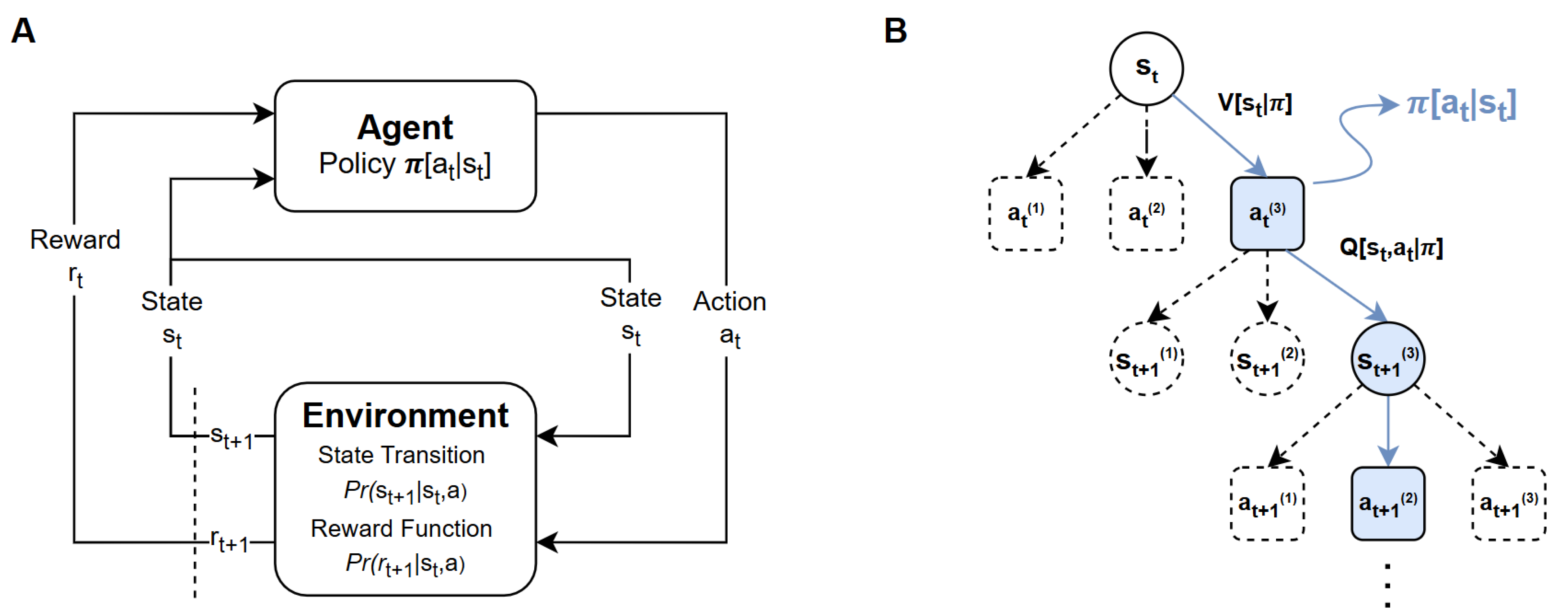
Reinforcement learning is grounded in sequential decision theory, originally formalized by Richard Bellman in the 1950s through dynamic programming. This theory gave rise to the general framework known as the Markov Decision Process (MDP), which forms the basis for a large family of RL algorithms [29]. Figure 1A illustrates the fundamental interaction structure between an agent and its environment: at each time instant t, the agent observes a state $s_t\in S$, selects an action $a_t\in A$ according to its policy $\pi \left(a_t\right|s_t)$, and receives a reward $r_t$ as the environment transitions to a new state $s_{t+1}$, according to a state transition probability function $Pr\left(s_{t+1}\right|s_t,a_t)$. Simultaneously, the reward function determines the distribution $Pr\left(r_{t+1}\right|s_t,a_t)$ governing the feedback from the environment and is therefore fundamental to the learning process.

The agent’s objective is to learn a policy $\pi :S\to A$ that maximizes the expected return, $G_t$ generally defined as the discounted sum of future rewards (see Equation (2)), where $\gamma \in [0,1]$ is the discount factor that weights the relative importance of future rewards. Values close to zero cause the agent to focus on immediate benefits, while values close to one promote decisions with a long-term perspective.

$$G_t=\sum _{t=0}^{\infty }{\gamma }^t{r}_{t+1}$$

(2)

Figure 1B schematically depicts the expansion of the decision tree from a state $s_t$. Each possible action $a_t^{\left(i\right)}$ from that state can lead to different future states $s_{t+1}^{\left(j\right)}$, and so on, generating multiple trajectories for the system evolution. In this framework, the policy $\pi \left(a_t\right|s_t)$ guides the selection of actions, while the quality of decisions can be evaluated using value functions. The state-value function $V\left(s_t\right|\pi )$ represents the expected cumulative reward when the agent starts from state $s_t$ and continues to act according to policy $\pi$. In contrast, the state-action value function $Q(s_t,a_t|\pi )$ represents the expected cumulative reward obtained when the agent first executes the action $a_t$ in state $s_t$ and then follows policy $\pi$. Intuitively, as shown in Figure 1B, $V\left(s_t\right|\pi )$ measures how desirable it is is to be in a given state under a policy, whereas $Q(s_t,a_t|\pi )$ measures how good it is to take a specific action in that state before continuing with the policy.

These functions form the core of RL algorithms, both in their classical tabular variants, such as Q-learning (off-policy) and SARSA (on-policy), and in their modern versions based on function approximators and deep neural networks. However, as the number of possible states and actions increases, the complexity of the decision space grows exponentially, posing significant challenges to designing optimal policies and formulating effective reward functions in partially observable or model-free environments.

2.3. Q-Learning

The mathematical formulation of reinforcement learning is based on the Bellman equation, which defines the optimal value of a policy recursively, decomposing the expected return as a function of future decisions. However, its classical formulation assumes full knowledge of the environment model, i.e., all transition probabilities and the reward function [29]. This limitation was overcome through the development of Temporal Difference (TD) methods, which allow the agent to learn directly from its experience when interacting with the environment [30].

The key principle of TD learning is the iterative update of value estimates through the temporal difference error ${\delta }_t$, which measures the discrepancy between predicted and observed returns. This principle has given rise to a broad family of bootstrapping algorithms [31], ranging from tabular methods such as Q-learning and SARSA, to intermediate formulations like Dyna-Q and AC, and modern deep reinforcement learning variants including Deep Q-Networks (DQN), PPO, DDPG, and Asynchronous Advantage Actor-Critic (A3C). Within this spectrum, the Q-learning algorithm [32] remains particularly relevant for its conceptual simplicity and practical robustness. Its update rule (see Equation (3)) is based on adjusting the value of a state-action pair based on both the immediate reward and the best estimated value of the next state. Importantly, Q-learning is classified as off-policy because, even if the agent explores the environment following a certain policy, the update always assumes that the best possible action will be taken in the future. The learning rate $\alpha \in [0,1]$ controls the extent to which new information influences the update, enabling the agent to progressively refine its estimates of the Q-function as it interacts with the environment.

$$Q(s_t,a_t)\leftarrow Q(s_t,a_t)+\alpha \underset{{\delta }_t}{\underbrace{\left[r_t+\gamma \underset{a_{t+1}}{max}Q(s_{t+1},a_{t+1})-Q(s_t,a_t)\right]}}$$

(3)

Under conditions of sufficient exploration and a sufficiently small learning rate, Q-learning has been shown to converge to the optimal value function $Q^{*}(s,a)$ [29]. However, the guaranteed convergence of Q-learning only holds under discrete and finite state and action spaces. To apply this algorithm to continuous control problems, such as PID tuning, requires performing an explicit discretization of the parameter space and possible observable values. This operation introduces a critical tension trade-off between accuracy and computational feasibility.

On the one hand, a coarse discretization reduces the size of the $Q(s,a)$ table, favoring the speed of learning and the use of lightweight architectures, but on the other hand, it limits the agent’s ability to approximate optimal solutions in continuous environments. Conversely, a fine discretization improves the resolution of the learned policy, but generates a combinatorial explosion of the state-action space, a phenomenon known as the “curse of dimensionality”, which can render learning impractical in terms of memory and convergence time.

In this context, Q-learning acquires strategic significance as a foundation for exploring the balance between simplicity and impact. Its explicit structure allows for a transparent analysis of how the agent’s decisions evolve based on the feedback obtained, which is especially valuable in tasks such as adaptive PID tuning, where understanding the interaction between local parameter settings and the global system response is essential.

2.4. RL Applied to PID Tuning

The integration of RL techniques with PID controllers has been widely studied, with deep reinforcement learning approaches being particularly prominent. Algorithms such as DDPG, PPO, and SAC have proven effective in continuous control tasks, where neural networks allow PID parameters to be adjusted based on experience, optimizing performance metrics such as cumulative error, overshoot, and robustness against disturbances [11,33,34,35]. In addition, architectures such as AC, A3C, and variants of PPO and DDPG have been applied in various scenarios, confirming the adaptability of deep RL to complex environments [17,36,37,38,39].

In parallel, hybrid schemes combining RL with heuristic techniques have been proposed. Among them, the use of fuzzy Q-learning in multi-agent systems has attracted particular attention, where each agent adjusts a PID parameter with rewards based on integral error indices (IAE, ITAE) [40]. Along the same lines, Li et al. [41] incorporated hybrid mechanisms capable of operating in continuous domains based on classical control performance metrics.

Conversely, discrete reinforcement learning algorithms have been effectively applied in robust predictive control models [42,43], integrated with other techniques for the adaptive management of actively perturbed environments, and for the tuning of PID controllers [44,45], although mainly under conditions of high observability and constrained methodological framework. Specifically, works such as those by Elhakim et al. [46], Shi et al. [47], and Thanh et al. [48] defined states based on error variables and their temporal evolution, while actions were defined actions as discrete increases or decreases in the gains. In these cases, reward functions penalized significant deviations and encouraged convergence toward stable configurations. Other proposals have introduced variants including incremental and double Q-learning approach, where the state space was progressively refined and the action space was adaptively expanded, using Gaussian rewards to improve reference tracking in mobile robotics [49,50]. In a similar framework, Fan et al. [51] applied Q-learning to trajectory tracking and lane guidance, and Yeh and Yang [52] compared Q-learning and SARSA with programmed actions in piezoelectric control scenarios, demonstrating the ability of these techniques to adapt the PID parameters in dynamic environments without requiring explicit system models.

Despite advances in the use of deep RL for PID controller tuning, there is still a lack of systematic studies evaluating the application of classical discrete algorithms, such as tabular Q-learning, in continuous systems, especially under limited observability conditions and without explicit models. This gap has been widened by the preference for high-resolution continuous approaches, which has limited the exploration of alternatives based on discretization. However, discrete methods offer advantages in terms of simplicity, interpretability, and consequently greater ease of implementation, which are relevant for industrial applications.

In this context, classical RL algorithms can be a viable alternative, provided critical aspects such as the reward function, exploration strategy, and action-space discretization are carefully defined. These considerations are fundamental to obtaining stable and reproducible policies. On this basis, this study revisits the role of discrete algorithms in the online tuning of PID controllers and proposes a multi-agent architecture based on Q-learning. The following section describes the methodology in detail and the proposed validation process, which combines episode training, specific reward functions, and a framework for evaluating training processes for transparent and interpretable algorithms.

3. Methodology

An experimental computational methodology based on episode-based simulation is adopted to enable the empirical evaluation of continuous dynamic control systems and to conceptually validate an integrated framework that combines a discrete RL scheme with classical PID control. The proposed approach aims to assess the feasibility of automatic gain tuning through decentralized multi-agent learning, applied to nonlinear systems of different orders.

The proposed control framework integrates a discrete multi-agent Q-learning scheme for the automatic tuning of PID controller gains in continuous dynamic systems. Each PID gain ($k_p$, $k_i$, $k_d$) is adjusted by an independent agent operating under low observability in a decentralized manner; that is, no agent directly observes the physical environment or exchanges information with other agents. The system is trained to achieve a single stabilization objective, relying solely on a global reward signal derived from the overall performance of the controlled system, without relying on explicit models or agent-specific reward functions.

3.1. State-Action Space

As described above, the state space of each agent is not defined by the physical variables of the dynamic system, but by the discrete set of possible values for its corresponding PID gain. The action space is the same for all agents and consists of three discrete options: decrease, maintain, or increase the current gain value. Actions that modify the gain produce a fixed change $\mathrm{\Delta }k$, which determines the granularity of the state-space discretization and is limited to an appropriate range of action. This design directs each agent to explore its gain space in search of combinations that simultaneously maximize the overall reward, thus indirectly identifying an effective control policy.

3.2. Training Plan

Training is structured into independent episodes with a fixed maximum duration. Each episode begins with the dynamic system in a perturbed state; all system variables are reset to predefined initial conditions, except for the agents learned Q-values, which accumulate across episodes. Within each episode, time is discretized into fixed-duration decision intervals $\mathrm{\Delta }{T}_{dec}$. At the beginning of each interval, every agent selects an action to update its respective gain. The selected gains remain fixed during that interval $\mathrm{\Delta }{T}_{dec}$ while the PID controller computes the control signal based on the current system error. The resulting control action is applied to the environment; the system dynamics are simulated by numerically integrating the corresponding differential equations, and the new environment state is obtained. The reward at each time step $dt$ is accumulated and used to update the agents Q-tables, allowing them to evaluate the cumulative impact of their actions before making subsequent decisions. Episode termination occurs when any of the following conditions is met:

1.

The maximum episode duration is reached.

2.

The system achieves stabilization according to predefined control thresholds.

3.

The deviation limits of the environment are exceeded.

If the episode ends prematurely, the final Q-value update excludes a temporal difference term, since no successor state exists; only the reward obtained up to that point is considered.

The learning process follows an off-policy framework that employs an $ϵ-\mathrm{greedy}$ exploration strategy with adaptive decay, enabling a gradual shift from exploration to exploitation as training progresses. Initially, a high $ϵ$ promotes active exploration of the reward space, while its gradual reduction progressively favors the exploitation of learned policies. Similarly, the learning rate $\alpha$ is adaptively decayed to stabilize Q-table convergence and to reduce sensitivity to recent observations during later stages of training.

3.3. Reward Function

The reward function, a key component of the proposed control framework, is computed at each decision interval as the sum of instantaneous rewards, which are in turn defined as an additive combination of multiple criteria reflecting both control performance and efficiency. The reward design guides the learning process toward PID gain configurations that maintain system stability while minimizing undesirable control actions.

The first component is the base reward $R_{base}$ (Equation (4)), which is modeled as a weighted Gaussian function centered at the desired operating point of n selected system variables. For each variable value $z_i$, ${\mu }_i$ denotes the setpoint value, ${\sigma }_i$ the sensitivity parameter that controls the curvature steepness, and $w_i$ the relative weight:

$$R_{base}=\sum _{i=1}^n{w}_i·exp\left(-{\displaystyle \frac{{(z_i-{\mu }_i)}^2}{2{\sigma }_i^2}}\right)$$

(4)

A time penalty, $P_t$ (Equation (5)), is applied at each step to encourage rapid stabilization and discourage excessively long episodes:

$$P_t=\alpha ·dt$$

(5)

where $\alpha$ is a proportionality constant.

An additional penalty $P_u$ is introduced to penalize abrupt changes in the control signal (Equation (6)). This term is modeled as a quadratic function of the control signal variation:

$$P_u=\beta ·{(u\left[t\right]-u[t-1])}^2$$

(6)

where $u\left[t\right]$ is the control action at the current step, $u[t-1]$ is the previous action, and $\beta$ a weighting factor.

To further encourage the agent to maintain the system within a desirable operating range, a per-step bandwidth bonus $R_{bw}$, is introduced (Equation (7)). This component provides a small constant reward whenever the observed variables remain within predefined limits of the target region.

$$R_{bw}=\left\{\begin{array}{cc}{r}_{bw},\hfill & \mathrm{if}{z}_j\in [{\widehat{\mu }}_j^{min}-{\delta }_j,{\widehat{\mu }}_j^{max}+{\delta }_j]\forall j\in \mathcal{B}\hfill \\ 0,\hfill & \mathrm{otherwise}\hfill \end{array}\right.$$

(7)

where $r_{bw}$ is the bonus magnitude, ${\widehat{\mu }}_j^{min}-{\delta }_j$ and ${\widehat{\mu }}_j^{max}+{\delta }_j$ denote the lower and upper bounds of the target range, respectively, and $\mathcal{B}$ denotes the set of variables for which the bandwidth condition is defined.

A goal-achievement bonus $R_{bonus}$ is granted when the system reaches the stabilization target (Equation (8)); otherwise, this bonus reward is set to zero:

$$R_{bonus}=\left\{\begin{array}{cc}300,\hfill & \mathrm{if}\mathrm{goal}=\mathit{True}\hfill \\ 0,\hfill & \mathrm{otherwise}\hfill \end{array}\right.$$

(8)

where $\mathrm{goal}=\mathit{True}$ when the target variables are within the predefined stabilization thresholds.

The total reward $R_t$ is accumulated over m time steps within each decision interval $\mathrm{\Delta }{T}_{dec}$, combining all active components of the instantaneous rewards as expressed in Equation (9):

$$R_t=\sum _{t=1}^m(R_{base}\left[t\right]-P_t\left[t\right]-P_u\left[t\right]+\left\{R_{bw}\left[t\right]\right|\mathit{if\; within\; bounds}\}+\left\{R_{bonus}\left[t\right]\right|\mathrm{if}\mathrm{goal}=\mathit{True}\})$$

(9)

3.4. Pseudocode

The core logic of the proposed training framework is summarized in Algorithm 1. The pseudocode formalizes the sequential process; from environment and agent initialization, through the episode loop and decision-interval cycle, to the Q-learning update stage, detailing the interactions among the simulation model, the PID controller, and the independent learning agents.

The pseudocode provides a structured representation of the proposed methodology, clarifying the operational flow and illustrating the integration of the PID controller with the decentralized multi-agent learning process.

Algorithm 1 Adaptive PID control in line with independent multi-agent Q-learning.
Nomenclature: $E_{max}\leftarrow$ Maximum number of episodes; ${\overrightarrow{x}}_0\leftarrow$ Physical initial conditions; $\mathbf{K}\leftarrow$ Controller gains; $\mathrm{\Delta }K\leftarrow$ Delta gain; $t\leftarrow$ Current time; $dt\leftarrow$ Integration time step; state_config←Discretize range of respective gains; $c_{dec}\leftarrow$ Decision counter; $a\leftarrow$ Actions (${\downarrow }_{\mathrm{\Delta }K}=0$, ${\downarrow \uparrow }_{\mathrm{\Delta }K}=1$, ${\uparrow }_{\mathrm{\Delta }K}=2$); $R_a\leftarrow$ Cumulative reward; ${\mathsf{\Pi }}_{ϵ}\leftarrow$$ϵ$-greedy policy; $\mathrm{\Delta }{T}_{dec}\leftarrow$ Interval decision time; $e\leftarrow$ Control variable error.
I. Episode Initialization:
The system is set to the initial state.
1: $Q_{tabl{e}_g}\leftarrow zeros(\overrightarrow{s},\overrightarrow{a})$	▷ Initialize learning matrix in zeros for each agent
2: for episode to $E_{max}$ do
3:   $\mathbf{x}\leftarrow {\overrightarrow{x}}_0$; $\mathbf{K}\leftarrow {\mathbf{K}}_0$; $t\leftarrow 0$; $done\leftarrow false$	▷ Initialize system parameters
4:   ${\mathcal{D}}_g\leftarrow initial\_agent\_state\left(stat{e}_{config}\right)$	▷ Create state space with function for
combinations
5:   for  $g\in \{p,i,d\}$ do
6:   $\overrightarrow{s}={\mathcal{D}}_g$; $\overrightarrow{a}=[1,1,1]$	▷ Initialize state-action space from initial conditions
7:   $c_{dec}\leftarrow 0$	▷ Initialize decision counter
II. Decision interval cycle:
Maintaining PID gains during the decision interval
8:   while not $done$ and $t<T_{max}$ do
9:   $R_a\leftarrow 0$	▷ Initialize cumulative reward
10:   for  $g\in \{p,i,d\}$ do
11:     $a_g\leftarrow {\Pi }_{ϵ}\left(s_g\right)$	▷ Select actions by $ϵ-\mathrm{greedy}$ strategy
12:     $K_g^{\prime }\leftarrow {\mathbf{K}}_{\mathbf{g}}+\mathrm{\Delta }K\left(a_g\right)$	▷ Calculate gains actions
13:     ${\mathbf{K}}_{\mathbf{g}}^{\prime }\leftarrow clipping(K_g^{\prime },K_g^{min},K_g^{max})$	▷ Apply limits to gains
14:     ${\mathbf{K}}_{\mathbf{g}}\leftarrow {\mathbf{K}}_{\mathbf{g}}^{\prime }$	▷ Apply controller gains for interval of each agent
15:     $s_g\leftarrow \mathcal{S}\left({\mathbf{K}}_{\mathbf{g}}\right)$	▷ Create state for each agent
16:   $N\leftarrow \lfloor \mathrm{\Delta }{T}_{dec}/dt\rfloor$	▷ Calculate steps for decision interval
17:   for $k=1$ to N do
18:     $u\leftarrow \mathcal{C}(e,\mathbf{K})$	▷ Calculate PID action control
19:     ${\mathbf{x}}^{\prime }\leftarrow \mathcal{F}(\mathbf{x},u,dt)$	▷ Calculate new state of dynamical system
20:     ${\mathbf{e}}^{\prime }\leftarrow {\mathbf{x}}^{\prime }-\mathbf{x}$	▷ Calculate new error of the system
21:     $t\leftarrow t+dt$	▷ Update time for each step
22:     $r\leftarrow \mathcal{R}({\mathbf{x}}^{\prime },u)$	▷ Calculate instantaneous reward
23:     $R_a\leftarrow R_a+r$	▷ Accumulate instantaneous reward
24:     $\mathbf{x}\leftarrow {\mathbf{x}}^{\prime }$	▷ Update new physical state for next iteration
25:     $done\leftarrow check\_termination(\mathbf{x},t)$	▷ Evaluate end of episode due to restrictions
or stabilization
26:     if $done$ then break
III. Update Q-Learning:
Update $Q_{table}$ using the cumulative reward
27:   for $g\in \{p,i,d\}$ do
28:     $s_g^{\prime }\leftarrow \mathcal{S}\left({\mathbf{K}}_{\mathbf{g}}\right)$	▷ Create new state for each agent
29:     $Q_{max}^{\prime }\leftarrow {max}_{a^{\prime }}{Q}_g(s_g^{\prime },a^{\prime })$
30:     if $done$ then $Q_{max}^{\prime }\leftarrow 0$
31:     $Q_g(s_g,a_g)\leftarrow Q_g(s_g,a_g)+\alpha (R_a+\gamma Q_{max}^{\prime }-Q_g(s_g,a_g))$	▷ Bellman TD
update equation
32:   if not $done$ then
33:     $c_{dec}\leftarrow c_{dec}+1$	▷ Update decision counter
34:     $\mathbf{e}\leftarrow {\mathbf{e}}^{\prime }$	▷ Update error of the system
IV. End of episode:
35:  $\mathrm{episode}\leftarrow \mathrm{episode}+1$	▷ Update number episode
36:  $ϵ\leftarrow max({ϵ}_{min},ϵ·decay)$; $\alpha \leftarrow max({\alpha }_{min},\alpha ·decay)$	▷ Update training parameters

4. Validation Tests

To validate the feasibility of the proposed framework, two classical nonlinear control problems are considered: level regulation of a water-tank (first-order system) and stabilization of an inverted pendulum on a moving cart (second-order system). Both problems are implemented in a closed-loop configuration using the Python 3.11.7 programming language. The system dynamics are modeled by differential equations and numerically solved using the fixed-step odeint integrator from the SciPy library. The complete source code, along with the datasets supporting the reported results, is publicly available on GitHub project repository (see Data Availability Statement). Additionally, the detailed parameter ranges and simulation values are provided in Appendix A (“Simulation parameters for each control problems”).

4.1. Level Control in Water-Tank

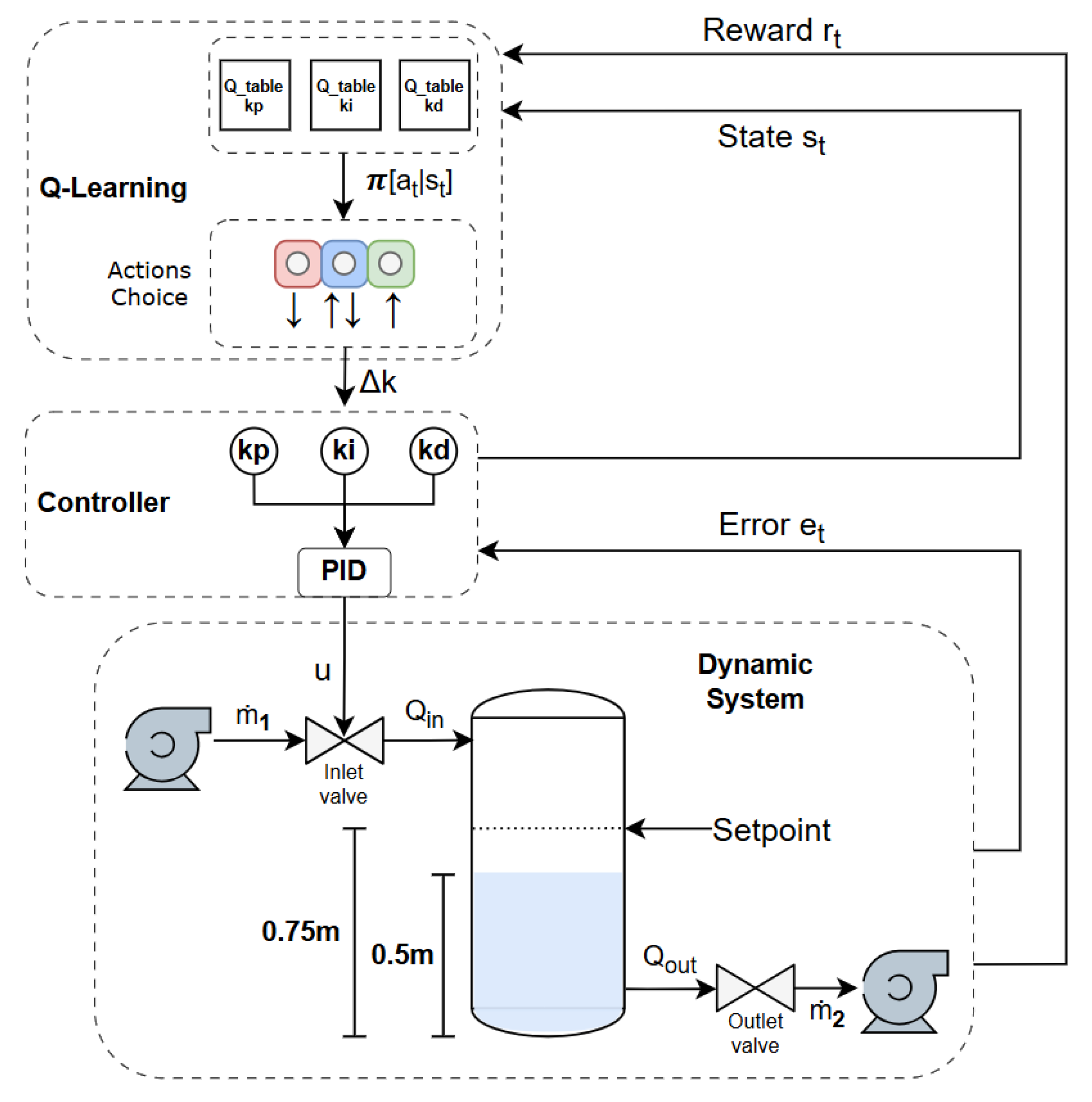
As shown in Figure 2, the first system consists of a hydraulic storage system supplied by an inlet pump delivering a fixed mass flow rate ${\dot{m}}_1$ and discharged through an outlet pump with a fixed mass flow rate ${\dot{m}}_2$. The liquid level is regulated by proportional valves located at the inlet and outlet pipes, positioned at the upper and lower ends of the tank, respectively. The outlet valve remains partially open at a constant ratio, determining the outlet volumetric flow $Q_{\mathrm{out}}$. The inlet valve, conversely, is dynamically adjusted by a PID controller to regulate the inlet volumetric flow $Q_{\mathrm{in}}$. The control objective is to achieve and maintain the liquid level at the reference setpoint, compensating for the continuous discharge through the outlet by modulating the inlet valve opening. The control signal u is bounded in $[0,1]$, directly determining the effective inflow to the tank.

The tank operates at atmospheric pressure $P_{\mathrm{atm}}$, is modeled as a vertical cylinder with constant cross-sectional area A$\left[m^2\right]$, and contains an incompressible fluid of uniform density $\rho$$[kg·m^{-3}]$. Temperature variations are neglected. The system dynamics based on the mass conservation principle relating inflow and outflow, is expressed in Equation (10):

$$A{\displaystyle \frac{\mathrm{d}h}{\mathrm{d}t}}=Q_{\mathrm{in}}-Q_{\mathrm{out}}$$

(10)

4.1.1. Training and Stabilization of Water-Tank

The training results show how the agents, guided by the $ϵ$-greedy exploration strategy and the designed reward function, progressively acquired policies capable of stabilizing the system under study. To evaluate this framework, global indicators are presented to track the evolution of the learning process: the distribution of episode termination reasons, cumulative performance per episode, and the stability achieved in the system response. These indicators provide an overall view of the progress achieved during the training and online tuning of the proposed system.

The training results show a transition from episodes dominated by time-based terminations to a predominance of successful stabilizations (Figure 3A). In the first iterations, most episodes did not meet the control criterion, reflecting the initial exploration phase; however, as learning progressed, the agents were able to identify gain configurations that allowed them to consistently reach the reference level. This progress is also observed in the evolution of the cumulative reward (Figure 3B), where the trajectories show a sustained increase and a reduction in variability, indicating more stable policies. The per-episode performance metric (Figure 3C) complements this behavior, showing an upward trend and convergence toward higher values, confirming improved temporal control efficiency. The dynamic behavior of the system is visualized using heat maps (Figure 3D–F). In Figure 3D, the time versus level curves initially show a wide dispersion around low values, followed by an increasingly dense grouping around the $0.74–0.75$ m range, reflecting a gradual convergence without sustained oscillations. This behavior is complemented by Figure 3E, which represents the relationship between the level and its rate of change, where the trajectories are distributed in positive slope fans for levels far from the target, reaching a maximum of $\dot{h}\approx 0.9$ and converging into different slopes as the level approaches the target value, indicating a varied exploration of the velocity profile while consistently applying the same approach strategy. This behavior is consistent with and explained by Figure 3F, which shows the temporal evolution of the control action, where the curve is characterized by an initial saturation toward the complete opening of the valve $u=1$, which allows for accelerated filling in the initial moments, followed by a gradual decrease until stabilizing within a narrower band around $u\approx [0.22–0.33]$. The reduction in variability in this region indicates that the controller reaches three stable steady states (where episodes accumulate), one central state exceeding 5 s and two adjacent states ending near 5 s.

4.1.2. PID Gains Regions of Stability in Water-Tank

The gain combinations leading to successful episodes reveal well-defined regions of the parameter space explored by the agents during training, a space where they learn stable and reproducible configurations due to the Q-learning algorithm’s gain maximization process.

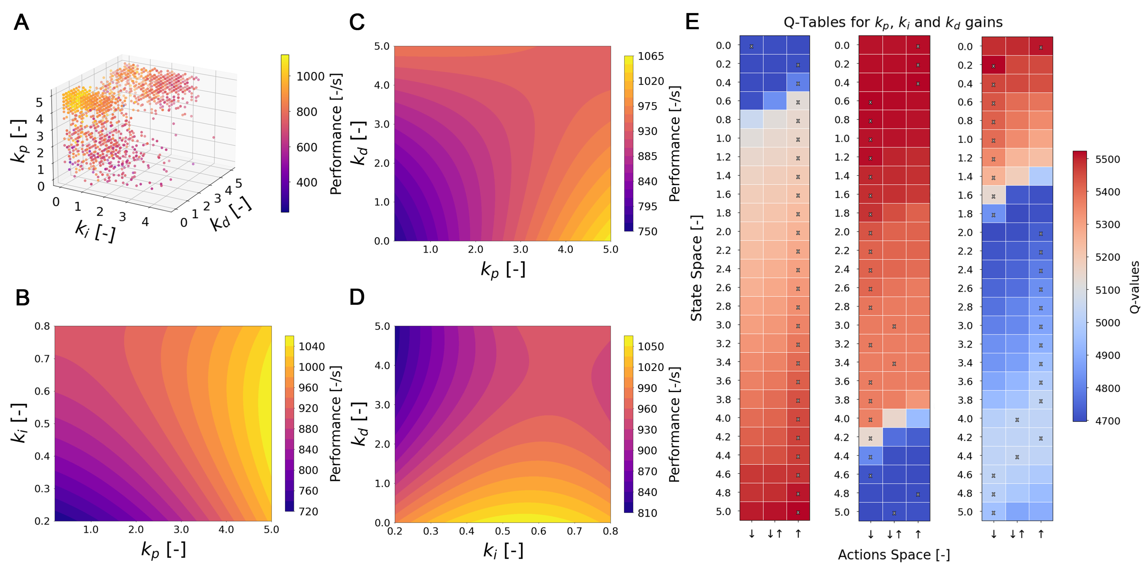
Figure 4A presents a three-dimensional scatter plot in which each point corresponds to a combination of $k_p$, $k_i$ and $k_d$ explored, color-coded according to the performance achieved. A heterogeneous distribution of configurations is observed, with a concentration of high performance values in the area associated with high proportional gains and low derivative and integral gains, indicating the presence of quasi-optimal regions where the controller effectively stabilizes the system. The stabilized region is subsequently modeled using second-degree polynomial curves (Specifically, $z=c_0+c_{1}x+c_{2}y+c_{3}xy+c_4{x}^2+c_5{y}^2$, with coefficients estimated by ordinary least squares.) for each pair of gains. Figure 4B shows the two-dimensional response surface for combinations of $k_p$ and $k_i$ with performance as the color metric. It exhibits an almost continuous gradient, showing that performance steadily improves as $k_p$ increases, particularly in the range $\in [4.0–5.0]$, while $k_i$ maintains a slight modulating effect in this area, limited to small values of $k_i\in [0.2–0.8]$.

Maximum performance occurs at $k_p=5.0$ and $k_i\in [0.4–0.8]$, confirming the dominant role of the proportional term in achieving stabilizing policies in this environment. Figure 4C represents the response surface for the $k_p–k_d$ plane, where broader regions (both gains $\in [0–5]$) are identified with moderate performance for a maximum value of $k_d$, but which decreases when combined with the absence of $k_p$ and increases if the latter reaches its maximum at $k_p=5.0$, confirming the dominant role of proportional gain in overall stabilization. Finally, Figure 4D illustrates the surface corresponding to the $k_i–k_d$ plane for the explored parameter spaces, with $k_d\in [0.0–5.0]$, while $k_i\in [0.2–0.8]$. In this case, the performance gradient indicates a plateau with average performance when both gains are high, and with a dependency distribution that favors reduced $k_d$ configurations, combined with a more indifferent $k_i$, but which peaks between the values $[0.4–0.7]$.

These visualizations reveal well-defined regions in the gain space where the controller achieves effective stabilization of the water-tank. The most favorable configurations are characterized by high values of the proportional gain, combined with low integral and derivative gains. This distribution suggests that the agent consistently converges toward a compact and reproducible region in the parameter space, guided by the design of the reward function and the defined stabilization objective. Consequently, the observed patterns emerge from the intrinsic optimization behavior of the Q-learning algorithm under these specific design constraints. It should be noted, however, that modifying the system parameters, operating ranges, or reward structure could lead to alternative regions in the gain space that also yield stable control policies.

4.1.3. Learned PID Policies in Water-Tank

The response surfaces discussed above indicate that the agent identifies a coherent subset of gain values capable of stabilizing the water-tank system. This is further confirmed by the analysis of the learned policies encoded in the Q-tables, which offer a transparent view of the agent’s preferences in the discretized state-action space. Figure 4E illustrates the distribution of learned actions across the gain space, providing visual confirmation of these tendencies.

For the water-tank system, the agent displays a clear preference for increasing the proportional gain $k_p$ toward its upper bound, reinforcing its critical role in the stabilization process. In contrast, the integral term $k_i$ tends toward low values that minimize cumulative error, though without clear convergence to a specific action. Instead, the agent fluctuates between slight increases and decreases within the narrow band around $k_i\in [0.4–0.6]$. Regarding the derivative gain $k_d$, the preferred actions concentrate in the lower portion of the discretized space. Although some exploratory behavior is observed for higher values of $k_d\in [4.0–4.4]$, these configurations are ultimately discarded, as the associated penalization for aggressive control signal variation leads to poorer long-term outcomes.

These findings confirm that the agent internalizes a policy aligned with the stability regions previously identified, converging on a compact and interpretable subset of the gain space conducive to robust control.

4.1.4. Fixed PID Gain Evaluation in Water-Tank

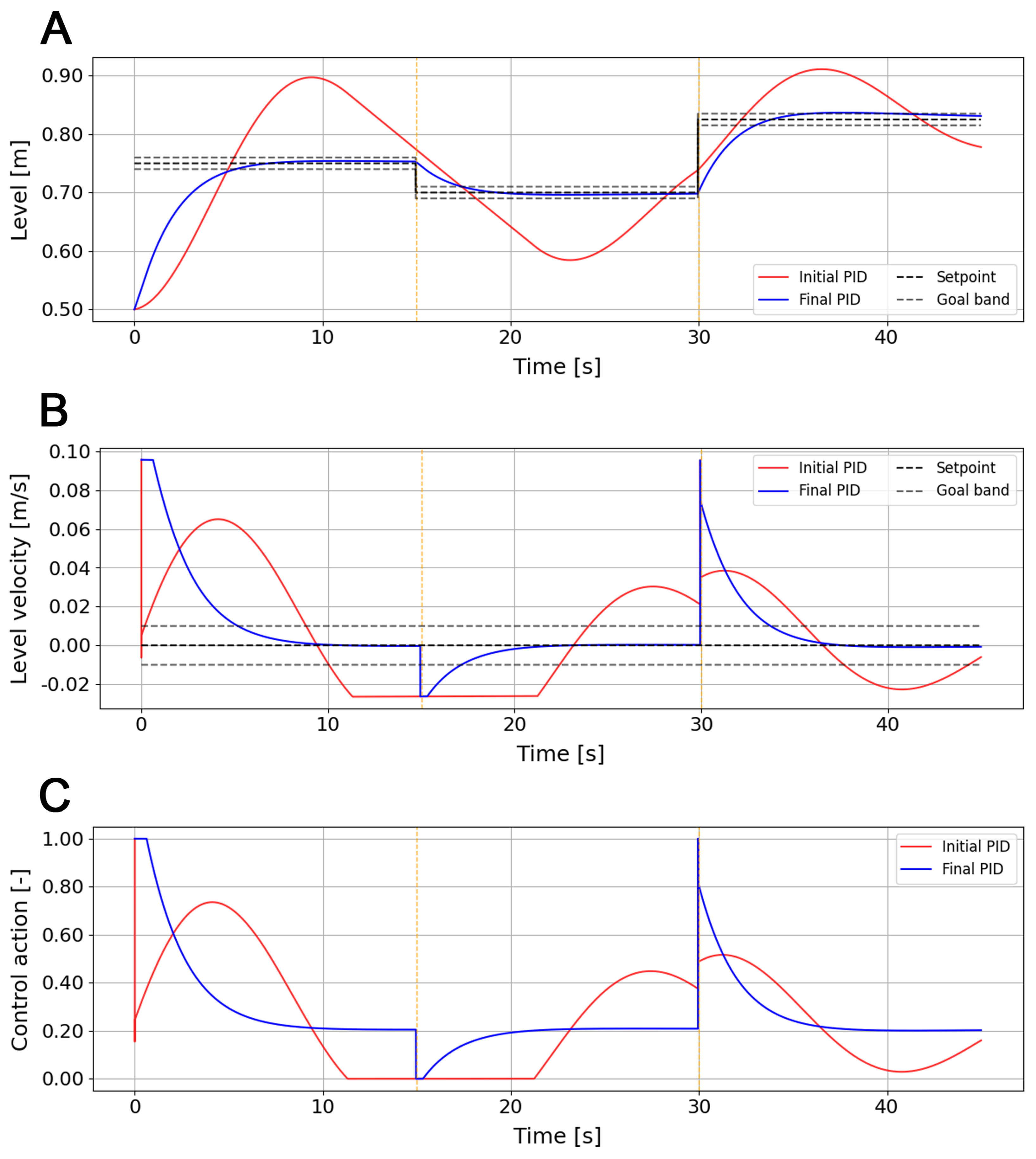
The fixed gains obtained in the final tuning stage, derived from the convergent policy in the Q tables ($k_p=5.0$, $k_i=0.5$ and $k_d=0.1$), were applied to the water-tank system during a 45 s episode in which the setpoint was sequentially varied to assess the tuned controller’s robustness. Figure 5 shows three reference levels applied in 15 s intervals, marked by orange vertical dashed lines, with a setpoint of $0.75$ m in the first interval, $0.7$ m in the next, and $0.825$ m in the last. The results are compared with the response of the initial PID controller ($k_p=1.0$, $k_i=1.0$ and $k_d=1.0$), both operating under identical conditions.

Figure 5A shows the level response. While the initial PID (red) shows a slow response after each setpoint change, a larger overshoot, and a lack of convergence, the final fixed PID (blue) achieves an immediate response to setpoint changes, a smooth transition, and stable convergence within the target band. This indicates a balanced gain configuration that minimizes error, avoids severe oscillations, and reduces steady-state deviations between consecutive setpoints, confirming the stability of the controller in response to the changes in operation. The corresponding level velocity shown in Figure 5B highlights the same behavior. The initial PID produces pronounced oscillations and an inadequate velocity response after each transition, while the final PID effectively attenuates these oscillations, resulting in a more critically damped response. The control action in Figure 5C further illustrates these differences. The initial PID shows noticeable fluctuations both within each interval and after each reference change, while the final PID maintains a moderate and constant control effort. The controller exhibits a rapid adjustment to the setpoint and a controlled opening or closing of the valve toward equilibrium at approximately $20\%$ of the outlet valve position, indicating that the learned gains achieve an effective balance between responsiveness and energy expenditure.

4.2. Stabilization of the Inverted Pendulum on a Cart

Also known as cart-pole system, Figure 6 depicts a planar (two-dimensional) setup consisting of a cart of mass $m_c$ moving horizontally with negligible friction and a pendulum of mass $m_p$ attached via a rigid, massless, and inextensible rod of length l. The control objective is to maintain the pendulum in the unstable inverted vertical position by applying a horizontal force F to the cart through an ideal linear actuator.

The dynamics are derived from the Newton-Euler equations, yielding a coupled nonlinear system of second-order differential equations that describe the cart’s motion and the pendulum angular oscillation. The equations, dependent on the pendulum angle $\theta$, angular velocity $\dot{\theta }$, cart position x, and cart velocity $\dot{x}$, are given in Equations (11) and (12), where g is the gravitational acceleration:

$${\displaystyle \frac{\mathrm{d}\dot{x}}{\mathrm{d}t}}={\displaystyle \frac{F+m_{p}sin\left(\theta \right)\left(l{\dot{\theta }}^2-gcos\left(\theta \right)\right)}{m_c+m_p{sin}^2\left(\theta \right)}}$$

(11)

$${\displaystyle \frac{\mathrm{d}\dot{\theta }}{\mathrm{d}t}}={\displaystyle \frac{-Fcos\left(\theta \right)-m_{p}l{\dot{\theta }}^{2}cos\left(\theta \right)sin\left(\theta \right)+(m_c+m_p)gsin\left(\theta \right)}{l\left(m_c+m_p{sin}^2\left(\theta \right)\right)}}$$

(12)

4.2.1. Training and Stabilization of Cart-Pole

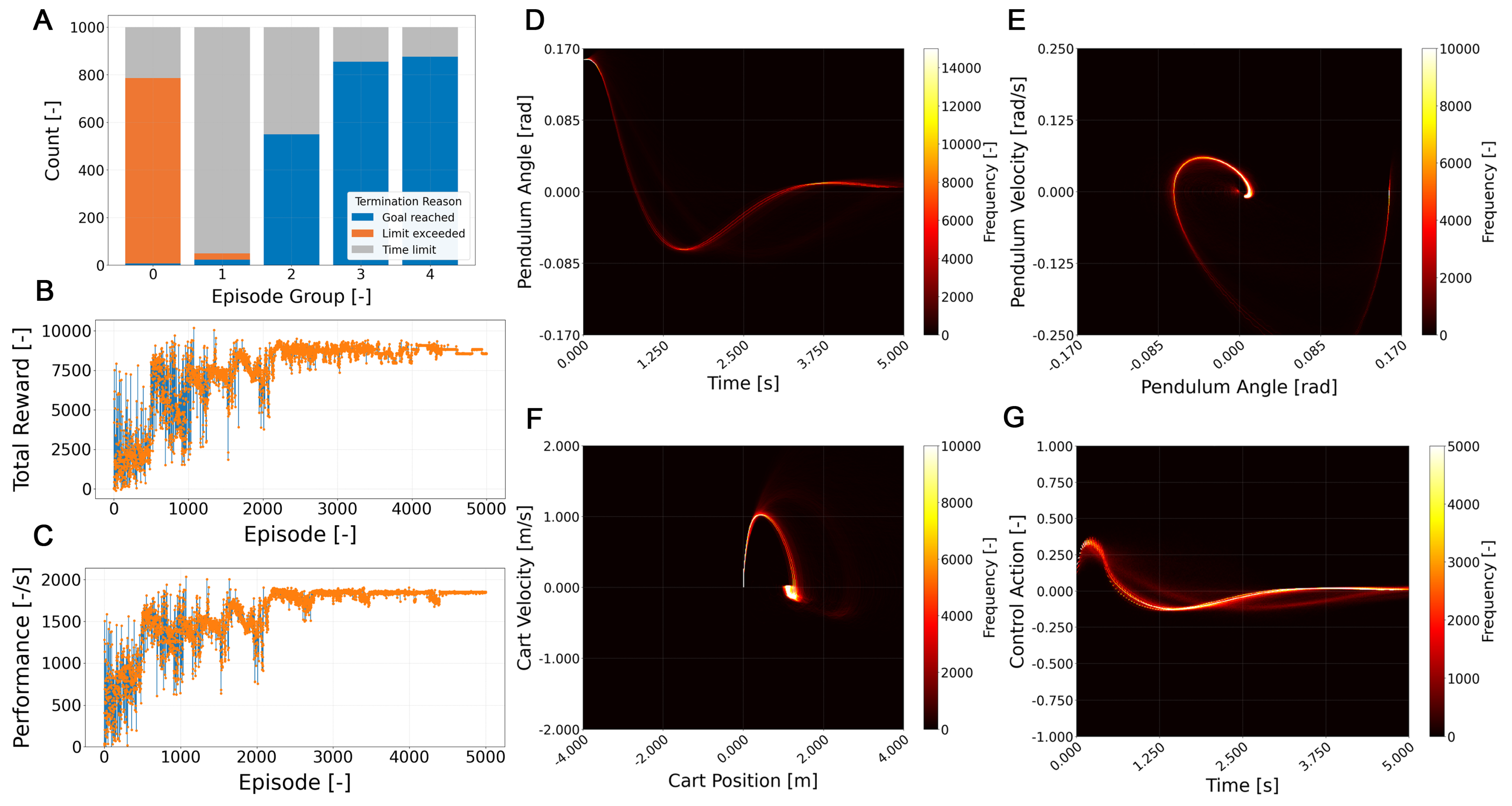
In the cart-pole system, the training evolution shows a progressive transition in the reasons for episode termination (Figure 7A). In the early stages, most attempts end due to exceeding position constraints or time limits, while in intermediate phases, a sustained increase in successful episodes is observed. In the last groups of episodes, the number of successful stabilizations far exceeds the number of failures, reflecting consistent exploitation of successful PID gain trajectories. This behavior is confirmed in the evolution of the accumulated reward per episode (Figure 7B), where the curves initially show high variability and low values, followed by a progressive increase until reaching a stable saturation level close to the maximum reward. The per-episode temporal performance metric (Figure 7C) exhibits a similar trend: an initially dispersed distribution with high amplitude that gradually converges to high and sustained values during the final episodes, within the shortest possible, reflecting a significant improvement in the agent’s ability to keep the pendulum in balance. The internal dynamics of the system is displayed in the heat maps (Figure 7D–G). In Figure 7D, corresponding to the angle of the pendulum with respect to time, there is a growing clustering around values close to equilibrium, with trajectories that gradually reduce the amplitude of oscillation and converge toward zero radians with no evidence of persistent oscillations. Figure 7E, which relates the angle to the angular velocity, shows a pattern characterized by trajectories concentrated around the origin, where the initial exploration fans collapse into a narrower and denser distribution, evidencing a reduction in the dispersion in the dynamic response of the pendulum. In Figure 7F, the phase space of the cart (position and velocity) initially shows wide and dispersed trajectories, followed by a progressive grouping around the central region, indicating more stable control of the base’s movement. Finally, Figure 7G, which represents the control action over time, reveals a response characterized by an initial broad effort that quickly reduces, stabilizing in a narrow band around the zero action ($u=0$). In addition, subtle trajectories can be seen in the control pattern, reflecting a transition from highly variable exploratory actions to more consistent and limited control signals that lead to pendulum stabilization and the cart detention.

4.2.2. PID Gains Regions of Stability in Cart-Pole

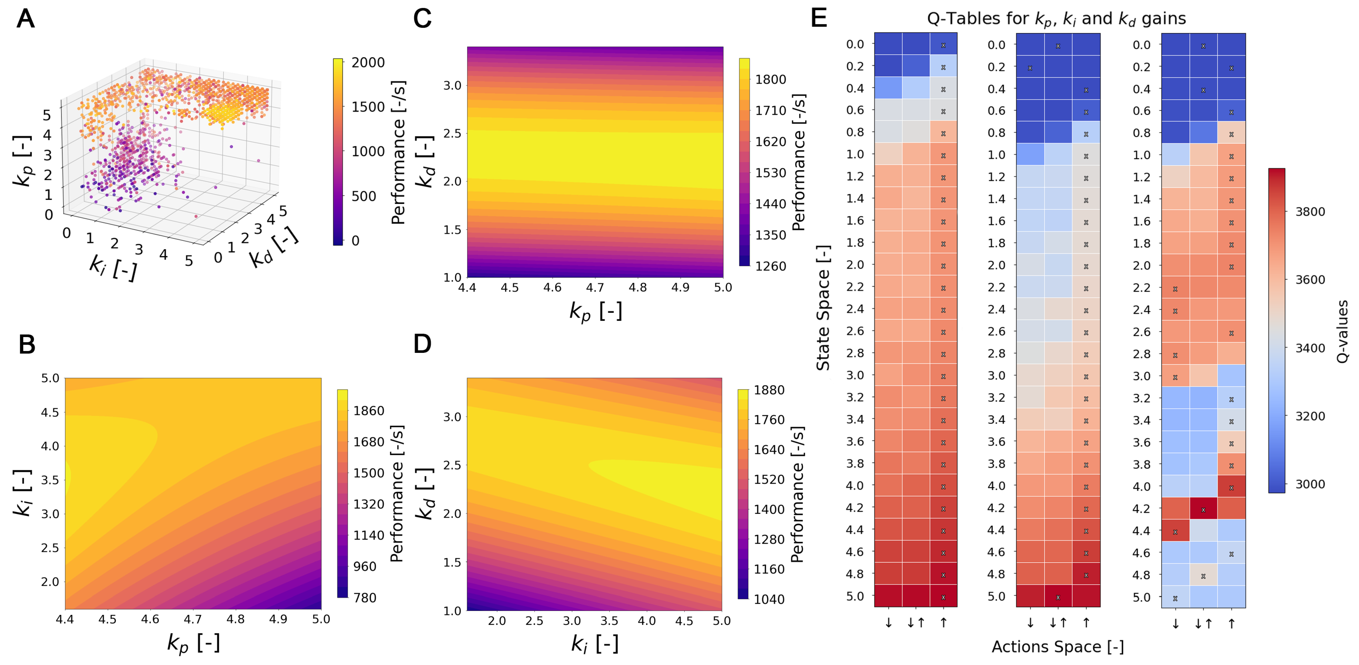
Figure 8A shows the three-dimensional distribution of the gain combinations explored during training. There is a wide dispersion in the parameter space, with a tendency toward higher performance values in regions where $k_p$ and $k_i$ reach high levels, while $k_d$ remains at intermediate values. This accumulation of episodes suggests the presence of a subset of successful gain configurations that favor system stabilization. Figure 8B illustrates the response surface in the $k_p–k_i$ plane, where positive gradients and low variability are observed for high values of $k_i$$\in [3.0–5.0]$, combined with any value within the range of $k_p\in [4.4–5.0]$, while the system rapidly deteriorates if $k_i<3.0$ and $k_p$ increases accordingly, indicating an important conditional dependence on high values of the integrative gain for the system.

For its part, the two-dimensional surface corresponding to the $k_p–k_d$ plane (Figure 8C) shows a convex gradient in performance, which is inherent to the proportional gain evaluation space, provided that the derivative gain is at an intermediate point. Specifically, the behavior can be represented as the surface of a truncated elliptical paraboloid, where maximum performance is achieved through a plateau throughout the entire range of $k_p\in [4.4–5.0]$, while the value of $k_d\in [2.0–2.5]$, otherwise performance declines progressively. This confirms that the combined and appropriate action of these gains contributes to a more stable control of the inverted pendulum, confirming the dominant role of the proportional and integral actions in correcting instantaneous and sustained errors over time, which are also critical for achieving rapid stabilization. Complementarily, Figure 8D, which relates $k_i$ and $k_d$, exhibits consistent behavior: performance increases for $k_d>2.0$ and reaches its maximum when $k_d\in [2.0–2.5]$ and $k_i>3.0$.

In contrast, the gain distributions explored in the cart-pole problem delineate a stability region that favors configurations with simultaneously high proportional and integral gains, alongside intermediate derivative values. This structure reflects the system’s sensitivity to both instantaneous and accumulated error, as well as the need for timely corrections. As with the water-tank, the stability regions found are compact and consistently reproducible, arising from the reward-driven optimization of policy learning. Nevertheless, these results are contingent upon the specific formulation of the control objective and reward function. Adjustments to these elements, or to the dynamic characteristics of the system itself, may redirect the learning process toward different, yet equally valid, regions of gain configurations.

4.2.3. Learned PID Policies in Cart-Pole

For the cart-pole system, the learned policies also exhibit convergence toward specific gain configurations that favor dynamic stability. The Q-tables, visualized in Figure 8E, reveal systematic preferences that mirror the stabilization trends observed in the response surfaces.

Both the proportional ($k_p$) and integral ($k_i$) terms exhibit ascending gradients toward their highest discretized values, confirming their combined importance in handling the cart-pole’s instability. The derivative gain $k_d$, however, shows a more nuanced pattern: action preferences concentrate around intermediate values $k_d\in [2.0–2.2]$, with an evident band of indecision suggesting the agent’s sensitivity to fine-tuning this parameter. Notably, an isolated peak at $k_d=4.2$ appears, but lacks continuity with the surrounding gradients, suggesting that it arises from early exploration rather than representing a robust control solution. This behavior likely stems from the system’s inherent instability, which initially incentivizes sharp corrective actions via high derivative terms—later refined as the learning algorithm stabilizes the policy.

Together, these patterns validate the agent’s ability to learn structured and system-specific control strategies that are consistent with previously identified stable gain regions, reinforcing the robustness of the proposed approach.

4.2.4. Fixed PID Gain Evaluation in Cart-Pole

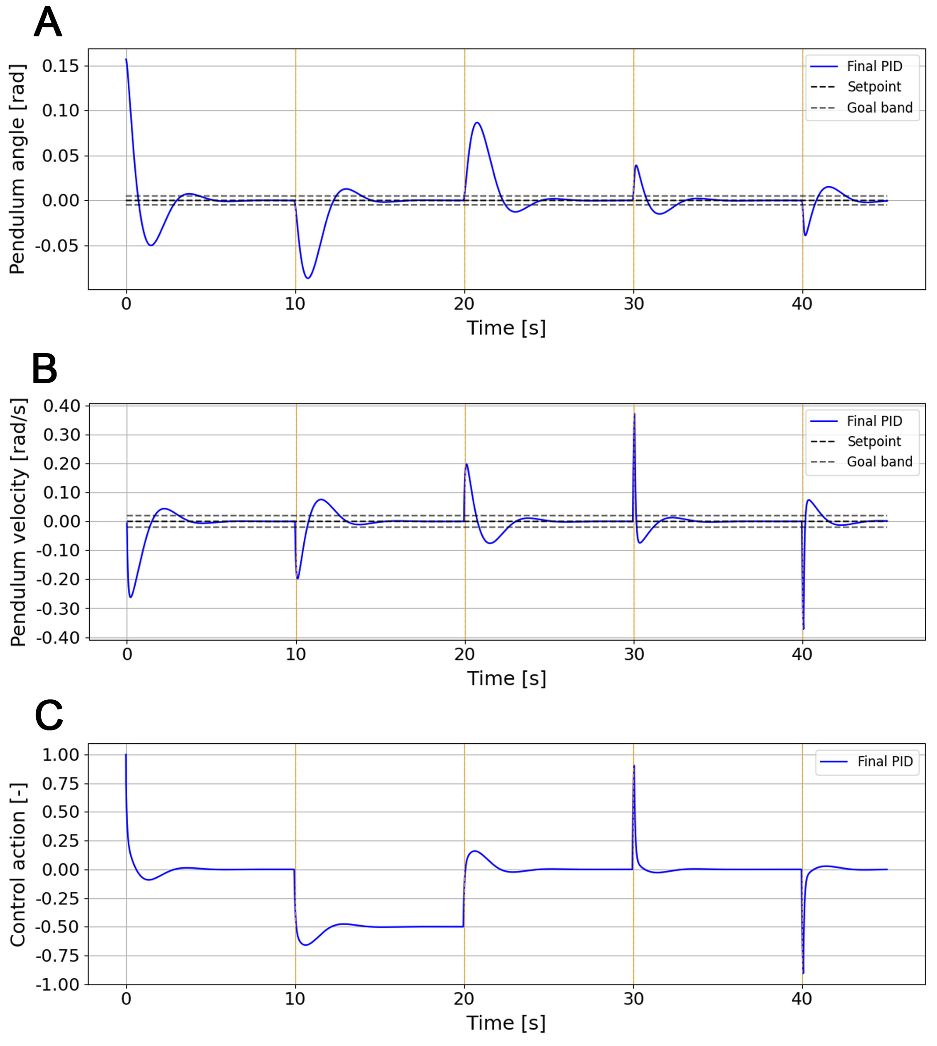
The fixed gains obtained from the final tuning ($k_p=5.0$, $k_i=5.0$ and $k_d=2.1$) were tested on the cart-pole system during a 45 s episode, maintaining the angle setpoint at $\theta =0$ to evaluate the controller’s ability to reject external disturbances in an inherently unstable system. Figure 9 illustrates how the system responds to different disturbance conditions: a constant positive step disturbance was applied to the cart at $50\%$ of the actuator capacity at 10 s and released at 20 s, followed by negative and positive impulse disturbances applied the maximum actuator capacity at 30 s and 40 s, respectively. For simplicity, only the pendulum angle, its angular velocity, and the control action are presented, since the cart displacement is not relevant to this analysis. The initial PID response is excluded, as it fails in the first interval and prevents proper comparison and evaluation of the final PID.

Figure 9A shows the evolution of the pendulum angle. Despite the sequence of disturbances, the final PID maintains the pole close to the upright position, with the angle deviation remaining within the target band after short transients. The system recovers with slight oscillations within the target band and an initial overshoot close to its limits, evidencing a fast recovery and effective disturbance rejection. The absence of sustained oscillations or drift highlights the stability of the fixed control law even under abrupt perturbations. The angular velocity response in Figure 9B complements this observation. Each disturbance generates a brief velocity peak that is quickly damped, demonstrating the controller’s ability to counteract both continuous and impulsive inputs without accumulating residual motion. This behavior confirms that the derivative action contributes to a well-damped transient, while the integral term efficiently restores the reference condition after the constant disturbance interval. Figure 9C shows the control effort applied by the final PID. The control action exhibits small oscillations; however, its magnitude remains within a safe operating range and consistent over time. After compensating for the deviation, the controller stabilizes by balancing the force on the cart at approximately $-50\%$ relative to the constant load step of the second interval. The control signal presents brief, limited peaks in response to external disturbances, with no evidence of saturation or sustained oscillation, reflecting a proportional balance between disturbance rejection and actuator economy.

Overall, the CartPole results validate the robustness of the fixed PID under external perturbations, maintaining upright stability through efficient and limited control effort. Together with the water-tank analysis, these results confirm that the fixed gains derived from the adaptive framework can sustain effective closed-loop behavior within bounded operational conditions. This capability supports the practical scalability of the approach, where adaptive learning can be complemented by stable fixed configurations for broader implementation across real control scenarios.

5. Discussion

The results confirm the feasibility of a multi-agent tabular scheme for online PID tuning under limited observability conditions. The findings of the proposed framework provide insight into the mechanism through which agents explore the gain space, converge toward reproducible configurations, and respond to reward function design.

Regardless of whether aggregate performance could be improved through finer-grained gain adjustments, the learned gain patterns align with the dynamic structure of each process. In the case of water-tank leveling, the predominance of high $k_p$ values accompanied by reduced $k_i$ and $k_d$ gains reflects the nature of a first-order system, where proportional action is sufficient to achieve a stable and rapid response without the need for significant integrative or derivative actions. This pattern contrasts with the cart-pole, an inherently unstable system that requires high $k_p$ and $k_i$ gains and an intermediate level of $k_d$ to effectively compensate for sustained error and moderate oscillations. These gains were obtained consistently (given the compact stability regions), demonstrating the agent’s ability to adapt to the specific dynamic requirements of each process.

As Jingliang Duan et al. [53] point out, the design of the reward function is a key factor in the stability and efficiency of learning. Poorly balanced rewards can induce undesirable behaviors, while carefully crafted functions facilitate more efficient learning trajectories and consistent results. Two operational design choices proved both decisive and scalable. First, the penalty for abrupt control action ($P_u$); in the case of the tank, it regulated the effective influence of the derivative, since its activation led to a brief initial saturation followed by stable valve behavior. Without the penalty, the agent tended to oversize $k_d$, generating undesirable initial oscillations. Second, in cart-pole, even when receiving only the angular error as feedback, the learned controller stabilized the pendulum and stopped the cart due to the reward design (Gaussian component on cart speed, operating bands, and goal bonus), internalizing implicit objectives without additional variables.

Additionally, the feasibility of the approach is further confirmed through analysis using fixed gains extracted from the converged Q-tables, where it is observed that with the same gains, the controller maintains its stabilizing capacity for references close to the training setpoint in both systems. Although extrapolation to targets or operating conditions far from the training range is not guaranteed, this suggests that the learned policies are not restricted to the training reference signal, a synergy that can be favorable in more complex proposals by preserving this capability of the PID algorithm.

Finally, it should be noted that the test environments are idealized, with perfect actuators and no internal or external disturbances, so scalability to more complex scenarios requires additional validation. Likewise, in order to scale the proposed framework, strategies and certain design challenges must be addressed, as they could directly affect system stability and convergence. On the one hand, the design of the state-action space as a discretization of gains is a limitation that affects both the identification of the status of the dynamic system itself and the fine tuning of the PID. A single-gain state representation was adopted to maximize interpretability and maintain the system’s modular applicability. Although closed-loop feedback carries environmental information, the agent’s perception remains partially observable, limiting context-dependent decisions in the event of large setpoint changes or unseen disturbances. Within the considered operating range, the readjustment procedure remains effective; however, extending the generalization would benefit from a hybrid state that increases discretized gains with critical loop variables, the inclusion of other agents that handle the context for adaptive control objectives, or adaptive discretization of gains [49]. However, care should also be taken when selecting the gain-change step size, since, together with the decision cadence, it imposes a resolution-efficiency trade-off that depends on both the sensitivity and the adjustment requirements of the system dynamics (longer windows for slow processes, immediate corrections for fast ones). On the other hand, sensitivity to hyperparameters, such as the reward, $ϵ-\mathrm{greedy}$ exploration rate, learning rate, and their decay schedules, must be carefully tuned according to the learning capacity and multi-agent configuration to avoid severe non-stationarity issues. These aspects represent key challenges that must be addressed before implementing the framework in more complex industrial applications or scaling it to higher-dimensional control problems.

6. Conclusions

The results demonstrate that the proposed multi-agent tabular Q-learning framework effectively performs online PID tuning under limited observability. In the water-tank control problem, the first signs of convergence appeared around 300 episodes, reaching full stability after approximately 2500–3000 episodes, where each of the last two groups of 1000 episodes consistently achieved success rates above $80\%$, maintaining a mean performance deviation below $5\%$. Over the complete 5000 episode training, $49.6\%$ of the runs reached the goal condition, while 50.4% ended due to time limit. In the cart-pole system, initial convergence emerged near 500 episodes and was consolidated around 2000–2500 episodes, where each of the last two groups of 1000 episodes exceeded $85\%$ successful stabilizations, with performance fluctuations below $5\%$. Across the full training horizon, $46.2\%$ of episodes were successful, $16.1\%$ failed due to exceeding physical limits, and $37.7\%$ terminated by time limit. These results confirm that independent agents can learn reproducible and stable gain configurations capable of sustaining continuous control without explicit process models.

The proposed framework provides a transparent and interpretable foundation for adaptive control, where the learning process can be examined directly in terms of PID gain evolution and the resulting control behavior. Its modular multi-agent design allows each component to operate independently, facilitating scalability toward more complex environments and enabling integration with analog PID architectures commonly used in industry. A key outcome of this study is the demonstrated influence of the reward function as a guiding mechanism for coordinated exploration, ensuring both stability and the emergence of desirable implicit behaviors such as minimizing control effort and maintaining safe operating ranges. This interpretability, together with the discrete and low-complexity nature of the scheme, positions the approach as a practical and scalable alternative for deployment in industrial environments requiring transparency, reliability, and explainable reinforcement learning control.

The evidence obtained not only confirms its feasibility but also highlights its potential as a research avenue for broadening the scope of RL applications in automatic control. Future work should focus on extending this framework toward more robust multi-agent systems capable of addressing intelligent adaptive control in complex industrial scenarios involving multiple controllers, strongly nonlinear dynamics, and diverse disturbance conditions. In addition, special attention should be paid to the design of advanced reward mechanisms, as the reward structure, together with fixed-gain decision intervals, proved essential in mitigating non-stationarity by allowing agents to perceive quasi-stationary environments. Therefore, in subsequent studies, it would be interesting to further investigate how these mechanisms contribute to stability, explore reward configurations and multi-objective formulations, and evaluate the impact of reducing observable parameters on convergence. Finally, assessing the feasibility and computational cost of the proposed approach on various integrated control platforms will be an essential step toward its practical implementation and validation under real operating conditions.

References

1. Hägglund, T. Process Control in Practice; De Gruyter: Berlin, Germany, 2023. [Google Scholar] [CrossRef]
2. Åström, K.J.; Hägglund, T. Advanced PID Control; ISA—The Instrumentation, Systems and Automation Society: Research Triangle Park, NC, USA, 2006. [Google Scholar]
3. da Silva, L.R.; Flesch, R.C.C.; Normey-Rico, J.E. Controlling Industrial Dead-Time Systems: When to Use a PID or an Advanced Controller. ISA Trans. 2020, 99, 339–350. [Google Scholar] [CrossRef]
4. Ogata, K. Modern Control Engineering, 5th ed.; Pearson: Upper Saddle River, NJ, USA, 2010. [Google Scholar]
5. Zhao, C.; Guo, L. Control of Nonlinear Uncertain Systems by Extended PID. IEEE Trans. Autom. Control. 2021, 66, 3840–3847. [Google Scholar] [CrossRef]
6. Joseph, S.B.; Dada, E.G.; Abidemi, A.; Oyewola, D.O.; Khammas, B.M. Metaheuristic Algorithms for PID Controller Parameters Tuning: Review, Approaches and Open Problems. Heliyon 2022, 8, e09399. [Google Scholar] [CrossRef]
7. Patil, R.S.; Jadhav, S.P.; Patil, M.D. Review of Intelligent and Nature-Inspired Algorithms-Based Methods for Tuning PID Controllers in Industrial Applications. J. Robot. Control. JRC 2024, 5, 336–358. [Google Scholar] [CrossRef]
8. Vartika, V.; Singh, S.; Das, S.; Mishra, S.K.; Sahu, S.S. A Review on Intelligent PID Controllers in Autonomous Vehicle. In Proceedings of the Advances in Smart Grid Automation and Industry 4.0; Reddy, M.J.B., Mohanta, D.K., Kumar, D., Ghosh, D., Eds.; Springer: Singapore, 2021; pp. 391–399. [Google Scholar] [CrossRef]
9. Prabhat Dev, M.; Jain, S.; Kumar, H.; Tripathi, B.N.; Khan, S.A. Various Tuning and Optimization Techniques Employed in PID Controller: A Review. In Proceedings of the International Conference in Mechanical and Energy Technology: ICMET 2019, Greater Noida, India, 7–8 November 2019; Yadav, S., Singh, D.B., Arora, P.K., Kumar, H., Eds.; Springer: Singapore, 2020; pp. 797–805. [Google Scholar] [CrossRef]
10. Diveev, A.; Sofronova, E.; Konstantinov, S.; Moiseenko, V. Reinforcement Learning for Solving Control Problems in Robotics. In Proceedings of the INTELS’22, Moscow, Russia, 14–16 December 2022; p. 29. [Google Scholar] [CrossRef]
11. Kranthi Kumar, P.; Detroja, K.P. Design of Reinforcement Learning Based PI Controller for Nonlinear Multivariable System. In Proceedings of the 2023 European Control Conference (ECC), Bucharest, Romania, 13–16 June 2023. [Google Scholar] [CrossRef]
12. Rajasekhar, N.; Radhakrishnan, T.; Samsudeen, N. Exploring Reinforcement Learning in Process Control: A Comprehensive Survey. Int. J. Syst. Sci. 2025, 56, 3528–3557. [Google Scholar] [CrossRef]
13. Sutton, R.S.; Barto, A. Reinforcement Learning: An Introduction, 2nd ed.; Adaptive Computation and Machine Learning; MIT Press: Cambridge, MA, USA; London, UK, 2020. [Google Scholar]
14. Sumiea, E.H.; Abdulkadir, S.J.; Alhussian, H.S.; Al-Selwi, S.M.; Alqushaibi, A.; Ragab, M.G.; Fati, S.M. Deep Deterministic Policy Gradient Algorithm: A Systematic Review. Heliyon 2024, 10, e30697. [Google Scholar] [CrossRef]
15. Guan, Z.; Yamamoto, T. Design of a Reinforcement Learning PID Controller. IEEJ Trans. Electr. Electron. Eng. 2021, 16, 1354–1360. [Google Scholar] [CrossRef]
16. Sass, Á.; Kummer, A.; Abonyi, J. Multi-Agent Reinforcement Learning-Based Exploration of Optimal Operation Strategies of Semi-Batch Reactors. Comput. Chem. Eng. 2022, 162, 107819. [Google Scholar] [CrossRef]
17. Shuprajhaa, T.; Sujit, S.K.; Srinivasan, K. Reinforcement Learning Based Adaptive PID Controller Design for Control of Linear/Nonlinear Unstable Processes. Appl. Soft Comput. 2022, 128, 109450. [Google Scholar] [CrossRef]
18. Glanois, C.; Weng, P.; Zimmer, M.; Li, D.; Yang, T.; Hao, J.; Liu, W. A Survey on Interpretable Reinforcement Learning. Mach. Learn. 2024, 113, 5847–5890. [Google Scholar] [CrossRef]
19. Li, P.; Fei, Q.; Chen, Z. Interpretable Multi-Agent Reinforcement Learning via Multi-Head Variational Autoencoders. Appl. Intell. 2025, 55, 577. [Google Scholar] [CrossRef]
20. Zabounidis, R.; Campbell, J.; Stepputtis, S.; Hughes, D.; Sycara, K.P. Concept Learning for Interpretable Multi-Agent Reinforcement Learning. In Proceedings of the 6th Conference on Robot Learning, Auckland, New Zealand, 14–18 December 2022; pp. 1828–1837. [Google Scholar]
21. Chi, R.; Lin, N.; Huang, B.; Hou, Z. Performance-Oriented Design and Analysis for Direct Data-Driven Control of Multi-Agent Systems. Inf. Sci. 2024, 666, 120419. [Google Scholar] [CrossRef]
22. Mi, X.; Liao, Y.; Zeng, H. Asynchronous Distributed Model Predictive Control for Multi-Agent Systems. IEEE Access 2025, 13, 9592–9605. [Google Scholar] [CrossRef]
23. Cappello, D.; Mylvaganam, T. Distributed Differential Games for Control of Multi-Agent Systems. IEEE Trans. Control. Netw. Syst. 2022, 9, 635–646. [Google Scholar] [CrossRef]
24. Matignon, L.; Laurent, G.J.; Fort-Piat, N.L. Independent Reinforcement Learners in Cooperative Markov Games: A Survey Regarding Coordination Problems. Knowl. Eng. Rev. 2012, 27, 1–31. [Google Scholar] [CrossRef]
25. Ziegler, J.G.; Nichols, N.B. Optimum Settings for Automatic Controllers. J. Dyn. Syst. Meas. Control. 1993, 115, 220–222. [Google Scholar] [CrossRef]
26. Cohen, G.H.; Coon, G.A. Theoretical Consideration of Retarded Control. Trans. Am. Soc. Mech. Eng. 2022, 75, 827–834. [Google Scholar] [CrossRef]
27. Åström, K.J.; Hägglund, T. PID Controllers: Theory, Design, and Tuning; ISA—The Instrumentation, Systems and Automation Society: Research Triangle Park, NC, USA, 1995. [Google Scholar]
28. Åström, K.J.; Hägglund, T. Automatic Tuning of Simple Regulators with Specifications on Phase and Amplitude Margins. Automatica 1984, 20, 645–651. [Google Scholar] [CrossRef]
29. Bellman, R. A Markovian Decision Process. Indiana Univ. Math. J. 1957, 6, 679–684. [Google Scholar] [CrossRef]
30. Sutton, R.S. Learning to Predict by the Methods of Temporal Differences. Mach. Learn. 1988, 3, 9–44. [Google Scholar] [CrossRef]
31. Sutton, R.; Barto, A. Reinforcement Learning: An Introduction. IEEE Trans. Neural Netw. 1998, 9, 1054. [Google Scholar] [CrossRef]
32. Watkins, C.J.C.H. Learning from Delayed Rewards. Ph.D. Thesis, King’s College, Cambridge, UK, 1989. [Google Scholar]
33. Yu, X.; Fan, Y.; Xu, S.; Ou, L. A Self-Adaptive SAC-PID Control Approach Based on Reinforcement Learning for Mobile Robots. Int. J. Robust Nonlinear Control. 2022, 32, 9625–9643. [Google Scholar] [CrossRef]
34. Song, L.; Xu, C.; Hao, L.; Yao, J.; Guo, R. Research on PID Parameter Tuning and Optimization Based on SAC-Auto for USV Path Following. J. Mar. Sci. Eng. 2022, 10, 1847. [Google Scholar] [CrossRef]
35. Liu, Y.; Jiang, X.; Li, X.; Sun, B.; Qian, S.; Wu, Y. Robot Target Tracking Control Considering Obstacle Avoidance Based on Combination of Deep Reinforcement Learning and PID. Proc. Inst. Mech. Eng. Part I J. Syst. Control. Eng. 2025, 239, 550–561. [Google Scholar] [CrossRef]
36. Shipman, W.J.; Coetzee, L.C. Reinforcement Learning and Deep Neural Networks for PI Controller Tuning. IFAC-PapersOnLine 2019, 52, 111–116. [Google Scholar] [CrossRef]
37. Park, J.; Kim, H.; Hwang, K.; Lim, S. Deep Reinforcement Learning Based Dynamic Proportional-Integral (PI) Gain Auto-Tuning Method for a Robot Driver System. IEEE Access 2022, 10, 31043–31057. [Google Scholar] [CrossRef]
38. Sun, Q.; Du, C.; Duan, Y.; Ren, H.; Li, H. Design and Application of Adaptive PID Controller Based on Asynchronous Advantage Actor–Critic Learning Method. Wirel. Netw. 2021, 27, 3537–3547. [Google Scholar] [CrossRef]
39. Hao, X.; Xin, Z.; Huang, W.; Wan, S.; Qiu, G.; Wang, T.; Wang, Z. Deep Reinforcement Learning Enhanced PID Control for Hydraulic Servo Systems in Injection Molding Machines. Sci. Rep. 2025, 15, 23005. [Google Scholar] [CrossRef]
40. Kofinas, P.; Dounis, A.I. Online Tuning of a PID Controller with a Fuzzy Reinforcement Learning MAS for Flow Rate Control of a Desalination Unit. Electronics 2019, 8, 231. [Google Scholar] [CrossRef]
41. Li, J.; Yao, Y.; Ma, N. Lane Following Method Based on Q-PID Algorithm. In Proceedings of the 2022 18th International Conference on Computational Intelligence and Security (CIS), Chengdu, China, 16–18 December 2022; pp. 38–42. [Google Scholar] [CrossRef]
42. Vegesna, A.V.; Shamaiah Narayanarao, M.; Bhamidipati, K.; Indiran, T. Q-Learning-Based Multivariate Nonlinear Model Predictive Controller: Experimental Validation on Batch Reactor for Temperature Trajectory Tracking. ACS Omega 2025, 10, 28362–28371. [Google Scholar] [CrossRef]
43. Zheng, Y.; Liu, Y.; Zeng, G.; Zhang, H.; Li, S.; Tang, Y.; Zhao, Q.; Luo, M.; Wang, Y. Distributed Q-Learning Model Predictive Control Based on ADMM for Continuous Nonlinear Systems. Digit. Chem. Eng. 2025, 16, 100257. [Google Scholar] [CrossRef]
44. Song, W.; Chen, Z.; Sun, M.; Sun, Q. Reinforcement Learning Based Parameter Optimization of Active Disturbance Rejection Control for Autonomous Underwater Vehicle. J. Syst. Eng. Electron. 2022, 33, 170–179. [Google Scholar] [CrossRef]
45. Li, L.; Song, K.; Tang, G.; Xue, W.; Xie, H.; Ma, J. Active Disturbance Rejection Path Tracking Control of Vehicles with Adaptive Observer Bandwidth Based on Q-learning. Control. Eng. Pract. 2025, 154, 106137. [Google Scholar] [CrossRef]
46. el Hakim, A.; Hindersah, H.; Rijanto, E. Application of Reinforcement Learning on Self-Tuning PID Controller for Soccer Robot Multi-Agent System. In Proceedings of the 2013 Joint International Conference on Rural Information & Communication Technology and Electric-Vehicle Technology (rICT & ICeV-T), Bandung, Indonesia, 26–28 November 2013; pp. 1–6. [Google Scholar] [CrossRef]
47. Shi, Q.; Lam, H.K.; Xiao, B.; Tsai, S.H. Adaptive PID Controller Based on Q-Learning Algorithm. CAAI Trans. Intell. Technol. 2018, 3, 235–244. [Google Scholar] [CrossRef]
48. Thanh, V.N.; Vinh, D.P.; Nam, L.H.; Nghi, N.T.; Le Anh, D. Reinforcement Q-learning PID Controller for a Restaurant Mobile Robot with Double Line-Sensors. In Proceedings of the 4th International Conference on Machine Learning and Soft Computing, ICMLSC’20, Haiphong City, Vietnam, 17–19 January 2020; pp. 164–167. [Google Scholar] [CrossRef]
49. Carlucho, I.; De Paula, M.; Villar, S.A.; Acosta, G.G. Incremental Q-learning Strategy for Adaptive PID Control of Mobile Robots. Expert Syst. Appl. 2017, 80, 183–199. [Google Scholar] [CrossRef]
50. Carlucho, I.; De Paula, M.; Acosta, G.G. Double Q-PID Algorithm Mob. Robot Control. Expert Syst. Appl. 2019, 137, 292–307. [Google Scholar] [CrossRef]
51. Fan, X.; Sui, J.; He, N.; Zhang, B.; Bu, C.; Yang, J.; Cui, L. Adaptive PID Trajectory Tracking Algorithm Using Q-Learning for Mobile Robots. In Proceedings of the 2022 12th International Conference on CYBER Technology in Automation, Control, and Intelligent Systems (CYBER), Baishan, China, 27–31 July 2022; pp. 1112–1117. [Google Scholar] [CrossRef]
52. Yeh, Y.L.; Yang, P.K. Design and Comparison of Reinforcement-Learning-Based Time-Varying PID Controllers with Gain-Scheduled Actions. Machines 2021, 9, 319. [Google Scholar] [CrossRef]
53. Duan, J.; Guan, Y.; Li, S.E.; Ren, Y.; Cheng, B. Distributional Soft Actor-Critic: Off-Policy Reinforcement Learning for Addressing Value Estimation Errors. IEEE Trans. Neural Networks Learn. Syst. 2022, 33, 6584–6598. [Google Scholar] [CrossRef] [PubMed]
Figure 1. (A) Agent-environment interaction within a Markov decision process. (B) Policy-based action selection tree illustrating the state-action-value relationship.
Mathematics 13 03461 g001
Figure 2. Control process of the water-tank level within the proposed Q-learning-based adaptive PID framework.
Mathematics 13 03461 g002
Figure 3. Training and performance results of the water-tank control system. (A) Distribution of episode termination reasons. (B) Cumulative reward per episode. (C) Performance metric (reward over final time) per episode. (D) Heatmap of water level over time. (E) Heatmap of water level versus level rate. (F) Heatmap of valve opening over time.
Mathematics 13 03461 g003
Figure 4. Analysis of PID gain optimization through Q-learning in the water-tank system. (A) Three-dimensional scatter plot of explored PID gain combinations and their corresponding performance values. (B) Response surface for proportional and integral gains ( k p k i ). (C) Response surface for proportional and derivative gains ( k p k d ). (D) Response surface for integral and derivative gains ( k i k d ). (E) Final Q-tables representing the discretized state-action spaces for proportional, integral, and derivative gains, highlighting the learned value distributions and optimal action selections.
Mathematics 13 03461 g004
Figure 5. Dynamic response of the water-tank system under the initial and optimized PID controllers. (A) Water level over time comparing initial and final PID configurations relative to the setpoints. (B) Water level rate over time for initial and optimized PID controllers. (C) Control effort over time showing the actuator response for initial and optimized PID controllers.
Mathematics 13 03461 g005
Figure 6. Control process of the cart-pole system within the proposed Q-learning-based adaptive PID framework.
Mathematics 13 03461 g006
Figure 7. Training and performance results of the cart-pole control system. (A) Distribution of episode termination reasons. (B) Cumulative reward per episode. (C) Performance metric (reward over final time) per episode. (D) Heatmap of pendulum angle over time. (E) Heatmap of pendulum angle versus angular velocity. (F) Heatmap of cart position versus cart velocity. (G) Heatmap of control action over time.
Mathematics 13 03461 g007
Figure 8. Analysis of PID gain optimization through Q-learning in the cart-pole system. (A) Three-dimensional scatter plot of explored PID gain combinations and their corresponding performance values. (B) Response surface for proportional and integral gains ( k p k i ). (C) Response surface for proportional and derivative gains ( k p k d ). (D) Response surface for integral and derivative gains ( k i k d ). (E) Final Q-tables representing the discretized state-action spaces for proportional, integral, and derivative gains, highlighting the learned value distributions and optimal action selections.
Mathematics 13 03461 g008
Figure 9. Dynamic response of the cart-pole system under external disturbance conditions with the fixed optimized PID controller. (A) Pendulum angle over time under different disturbance scenarios. (B) Pendulum angular velocity over time under different disturbance scenarios. (C) Control action over time showing the controller’s response to the applied disturbances.
Mathematics 13 03461 g009
Disclaimer/Publisher’s Note: The statements, opinions and data contained in all publications are solely those of the individual author(s) and contributor(s) and not of MDPI and/or the editor(s). MDPI and/or the editor(s) disclaim responsibility for any injury to people or property resulting from any ideas, methods, instructions or products referred to in the content.