An Attention-Driven Hybrid Deep Network for Short-Term Electricity Load Forecasting in Smart Grid

Abstract

With the large-scale development of smart grids and the integration of renewable energy, the operational complexity and load volatility of power systems have increased significantly, placing higher demands on the accuracy and timeliness of electricity load forecasting. However, existing methods struggle to capture the nonlinear and volatile characteristics of load sequences, often exhibiting insufficient fitting and poor generalization in peak and abrupt change scenarios. To address these challenges, this paper proposes a deep learning model named CGA-LoadNet, which integrates a one-dimensional convolutional neural network (1D-CNN), gated recurrent units (GRUs), and a self-attention mechanism. The model is capable of simultaneously extracting local temporal features and long-term dependencies. To validate its effectiveness, we conducted experiments on a publicly available electricity load dataset. The experimental results demonstrate that CGA-LoadNet significantly outperforms baseline models, achieving the best performance on key metrics with an $R^2$ of 0.993, RMSE of 18.44, MAE of 13.94, and MAPE of 1.72, thereby confirming the effectiveness and practical potential of its architectural design. Overall, CGA-LoadNet more accurately fits actual load curves, particularly in complex regions, such as load peaks and abrupt changes, providing an efficient and robust solution for short-term load forecasting in smart grid scenarios.

1. Introduction

The traditional power grid is a linear system in which electricity is transmitted unidirectionally from centralized power plants to end users through high-voltage transmission lines [1,2]. However, with the rapid advancement of the socio-economic environment, modern power systems have become increasingly complex. Electricity demand continues to rise, and their operational characteristics now exhibit stronger nonlinearity, temporal dependence, and volatility. Specifically, the power transmission path is fixed and lacks bidirectional interaction between the generation and consumption sides [3]. Moreover, the terminal sections of the grid lack effective real-time monitoring and control mechanisms, which restricts the ability to respond promptly to user behavior changes and load fluctuations [4,5].

To overcome these limitations, the smart grid (SG) has emerged as a next-generation power system [6]. It integrates advanced information and communication technologies with intelligent control mechanisms, and it places greater emphasis on high-precision electricity load forecasting [7,8]. Accurate load forecasting enables adaptive grid operation, refined control, and efficient electricity market mechanisms. It also provides essential support for renewable energy integration, electricity pricing optimization, and demand-side management [9]. Therefore, short-term load forecasting (STLF) has become one of the core research tasks in modern smart grids.

In the field of electricity load forecasting, traditional methods primarily rely on statistical models, such as ARIMA, linear regression, or empirical rules [10,11]. These approaches face difficulties in modeling non-stationary behaviors, local peaks, and multi-scale fluctuations in load data, leading to limited forecasting accuracy and insufficient timeliness for modern smart grid applications [12]. Deep learning methods, such as recurrent neural network (RNN), long-short term memory (LSTM), and gated recurrent units (GRUs), have enhanced the capability of modeling complex time series [13]; however, they still struggle with long-sequence dependency modeling, limited sensitivity to local patterns, and constrained generalization performance [14]. Consequently, there remains a research gap for a model that can simultaneously capture local temporal patterns, long-term dependencies, and adaptively focus on critical time steps to enhance prediction stability and accuracy.

To address these challenges, we propose a hybrid deep learning model, CGA-LoadNet, which integrates a one-dimensional convolutional neural network (1D-CNN), GRUs, and self-attention mechanisms. The model combines the advantages of a CNN for local feature extraction, GRUs for long-term dependency modeling, and self-attention for dynamically focusing on critical time steps. Experimental validation on public load datasets demonstrates that CGA-LoadNet significantly outperforms RNN, LSTM, GRUs, and their convolutional fusion variants in metrics such as the coefficient of determination ($R^2$), root mean square error (RMSE), mean absolute error (MAE), and mean absolute percentage error (MAPE), showcasing superior prediction accuracy and robustness, as well as practical applicability. The innovation and novelty of our scheme are summarized as follows.

(1)

We propose CGA-LoadNet, a hybrid deep learning model that addresses nonlinearity, multi-scale fluctuations, and high-frequency variations in STLF by combining a CNN, GRUs, and self-attention.

(2)

Comprehensive experiments on a public electricity load dataset show that CGA-LoadNet achieves the best performance in $R^2$, RMSE, MAE, and MAPE among all comparison models, demonstrating robust and accurate forecasting capability.

This section provides an overview of the electric load forecasting, and the following sections in this paper are structured as follows. Section 2 describes the related work on methods for electric load forecasting. Section 3 presents the proposed CGA-LoadNet approach and provides an overview of the comparative methods. Section 4 illustrates the experimental configurations. It contains a description of the dataset, the data preprocessing, and the evaluation metrics used in this study. Section 5 illustrates the experimental results and compares them with previous studies. Section 6 provides the conclusions of this paper.

2. Related Work

In recent years, the rapid development of deep learning and intelligent optimization techniques has significantly advanced the field of short-term electricity load and energy consumption forecasting. Research has predominantly focused on exploring various model architectures, particularly in terms of their time-series modeling capabilities and prediction accuracy. These models include CNNs, RNNs, LSTMs, Transformer architectures, and integrated optimization algorithms.

Yazıcı et al. [15] compared 1D-CNN, LSTM, and GRU models for short-term load forecasting based on real electricity consumption data. Their work demonstrated the effectiveness of 1D-CNN models for practical application scenarios. Xue et al. [16] developed an energy consumption forecasting scheme tailored for IoT environments. By leveraging deep neural networks and real-time device data, their model enhanced the accuracy of predicting building energy consumption trends through the fusion of historical and current information.

To address the challenge of joint multi-energy forecasting in integrated energy systems, Wang et al. [17] proposed MultiDeT, a multi-decoder Transformer-based model that enables joint prediction of multiple energy carriers within a unified encoder framework. Huang et al. [18] proposed a hybrid inverted Transformer model for short-term regional energy system forecasting, integrating a two-stage feature extraction mechanism. Their method effectively captured both temporal dependencies and cross-regional feature interactions, leading to improved forecasting performance for smart energy systems. Lu et al. [19] introduced QR-Parallel CNN-BiGRU, a hybrid model that combines quantile regression with parallel convolutional and bidirectional GRU networks, along with an improved whale optimization algorithm for hyperparameter tuning, enabling accurate 24 h probabilistic load forecasting and uncertainty quantification for smart grid operations. Kim et al. [20] proposed a hybrid CNN-LSTM model for residential load forecasting, where the CNN extracts spatial (multi-variable) features and the LSTM captures temporal dependencies; the network achieved significantly lower RMSE compared to traditional models across real-world household energy datasets. Abbas et al. [21] proposed SADE-KAN, a hybrid framework combining Kolmogorov–Arnold Networks with a self-adaptive differential evolution algorithm for short-term load forecasting. This model achieved high-precision, short-term forecasting while significantly reducing the number of parameters, making it especially suitable for multi-timescale load prediction tasks. Wen et al. [22] proposed a deep learning-driven hybrid model for short-term load forecasting, integrating Temporal Convolutional Networks, GRU units, and an attention mechanism. Their approach effectively captured both local temporal patterns and long-term dependencies, achieving high prediction accuracy.

In summary, recent studies have demonstrated that deep learning-based hybrid architectures, such as CNN-RNN, CNN-GRU, and attention-enhanced networks, can effectively capture temporal patterns and improve short-term load forecasting accuracy. Meanwhile, Transformer-based models, including both standard and hybrid variants, have emerged as a powerful alternative due to their ability to model long-range dependencies and multi-scale interactions more effectively. However, despite their growing importance, Transformer approaches may entail higher computational costs and data requirements, making hybrid CNN-, GRU-, and attention-based frameworks a competitive solution in scenarios that demand both efficiency and accuracy. To provide a concise overview of representative studies, we summarize their models, datasets, and forecasting horizons in

Table 1. Summary of studies in load and energy forecasting.

Authors	Model/Method	Dataset/Domain	Forecast Horizon
Yazıcı et al. [15]	1D-CNN, LSTM, GRU	Real electricity consumption data	Short-term
Xue et al. [16]	CNN-BiLSTM hybrid	IoT-based building energy data	Building-level energy consumption
Wang et al. [17]	MultiDeT	Integrated energy systems	Multi-energy joint forecasting
Huang et al. [18]	Hybrid Inverted Transformer	Regional smart energy systems	Short-term load forecasting
Lu et al. [19]	QR-Parallel CNN-BiGRU	Smart grid load data	24 h probabilistic forecasting
Kim et al. [20]	CNN-LSTM hybrid	Household energy datasets	Residential short-term load
Abbas et al. [21]	SADE-KAN	Multi-timescale load data	Short-term/multi timescale
Wen et al. [22]	CNN-GRU-Attention	Public electricity datasets	Short-term

. These limitations and trends motivate our work to develop a hybrid model capable of extracting local features, modeling long-term dependencies, and dynamically focusing on critical time steps.

3. Methodology

This section provides an overview of the preliminary work on our proposed CGA-LoadNet approach and comparative methods.

3.1. Preliminaries

The subsection provides essential background definitions. It establishes a clear foundation for the proposed approach and facilitates comprehension of the subsequent methodology and results.

3.1.1. One Dimension CNNs (1D-CNNs)

Electricity load data exhibit significant temporal characteristics, and they are often accompanied by local periodic fluctuations and irregular disturbances, which are particularly evident in daily load variations and peak consumption periods. These local patterns play a critical role in determining the accuracy of load forecasting models. To effectively capture such features, this study adopted a 1D-CNN to model the input sequences. By sliding one-dimensional convolutional kernels along the time axis, 1D-CNN can automatically extract local dependencies and key temporal patterns from the data, as shown in Figure 1. Compared to traditional handcrafted feature engineering methods, 1D-CNN offers advantages, such as end-to-end training, parameter sharing, and local receptive fields, thereby improving modeling efficiency and enhancing both generalization ability and forecasting performance.

3.1.2. Recurrent Neural Networks (RNNs)

RNNs are a class of neural network architectures specifically designed for modeling sequential data. By transmitting hidden states across time steps, RNNs are capable of capturing temporal dependencies within a sequence. Compared with traditional feedforward neural networks, RNNs incorporate a memory mechanism that allows the model to retain historical information and learn the dynamic evolution patterns of data over time. In tasks such as electricity load forecasting, RNNs can effectively learn temporal patterns from historical load sequences and demonstrate strong modeling capabilities.

3.1.3. Long Short-Term Memory (LSTM) Networks

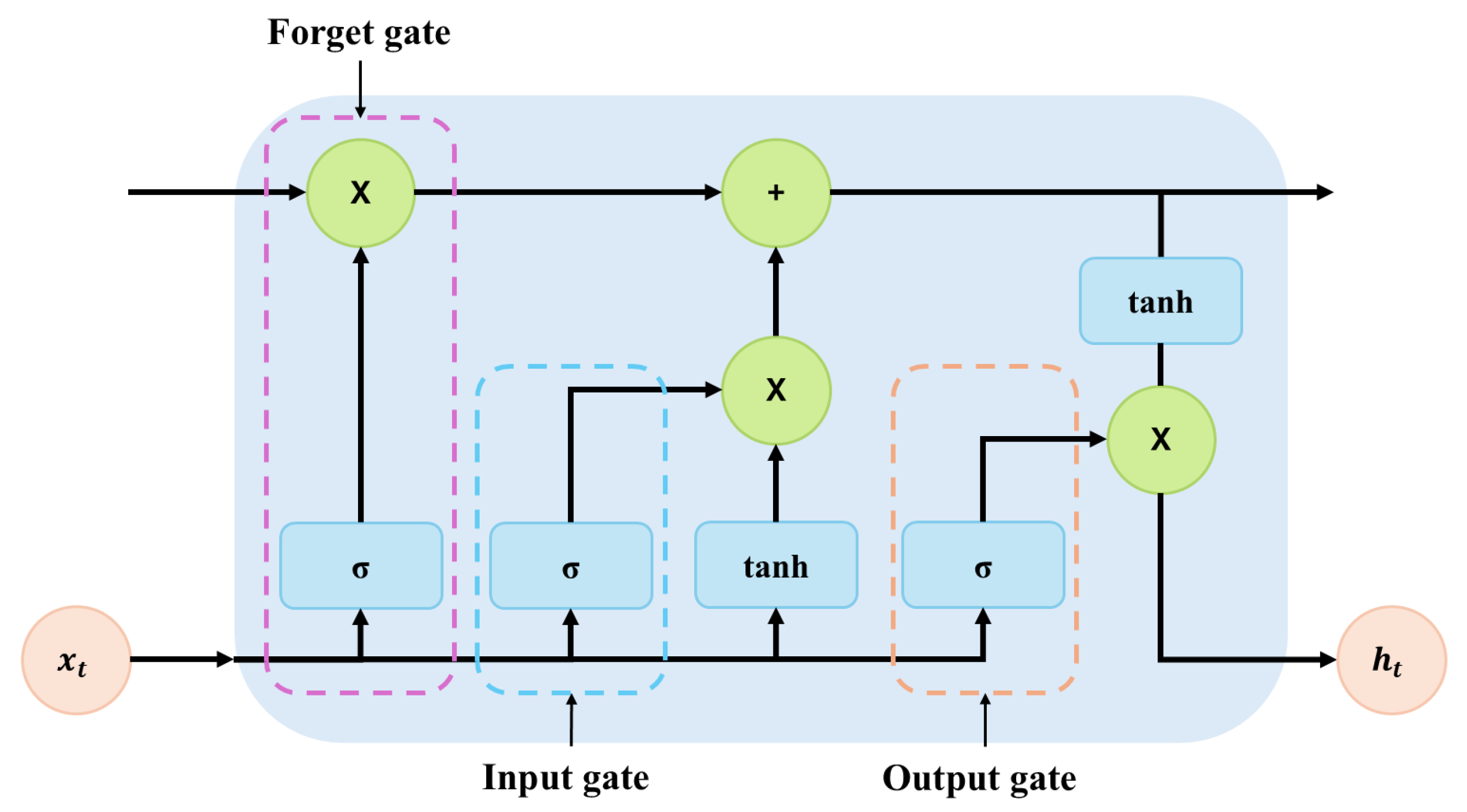
To address the problem of gradient vanishing in traditional RNNs when modeling long-term dependencies, LSTM was introduced. By incorporating gated mechanisms, such as the forget gate, input gate, and output gate, LSTM can effectively retain key information over extended time sequences. (The LSTM structure is shown in Figure 2). In recent years, LSTM has been widely applied in time-series modeling tasks such as electricity load forecasting, particularly excelling at capturing long-term trends and periodic patterns in load variation.

3.1.4. Gated Recurrent Unit (GRU)

The GRU is a simplified variant of LSTM, as shown in Figure 3. It merges the forget gate and input gate into a single update gate and omits the separate memory cell, thereby reducing the number of model parameters while retaining temporal modeling capability. Due to its lower structural complexity, GRU generally offers higher training efficiency and faster convergence, making it particularly suitable for modeling short- and medium-term time series. In the context of this study on electricity load forecasting, GRU can effectively capture dynamic changes and periodic patterns in the sequence, thereby improving prediction accuracy and model stability.

3.1.5. Self-Attention

The self-attention mechanism, initially developed for natural language processing, has in recent years been extended to various time-series modeling tasks. In the context of electricity load forecasting, the attention mechanism calculates importance scores for each time step in the input sequence, enabling weighted representation of key information segments and thereby enhancing the focus of feature extraction. Compared with traditional recurrent neural network architectures, the attention mechanism overcomes the limitation of fixed context windows, explicitly models long-term dependencies, and strengthens the perception of global contextual information. Moreover, integrating attention with models such as CNNs and GRUs can further improve the representational and predictive capabilities for complex load sequences.

3.2. Our Proposed CGA-LoadNet Approach

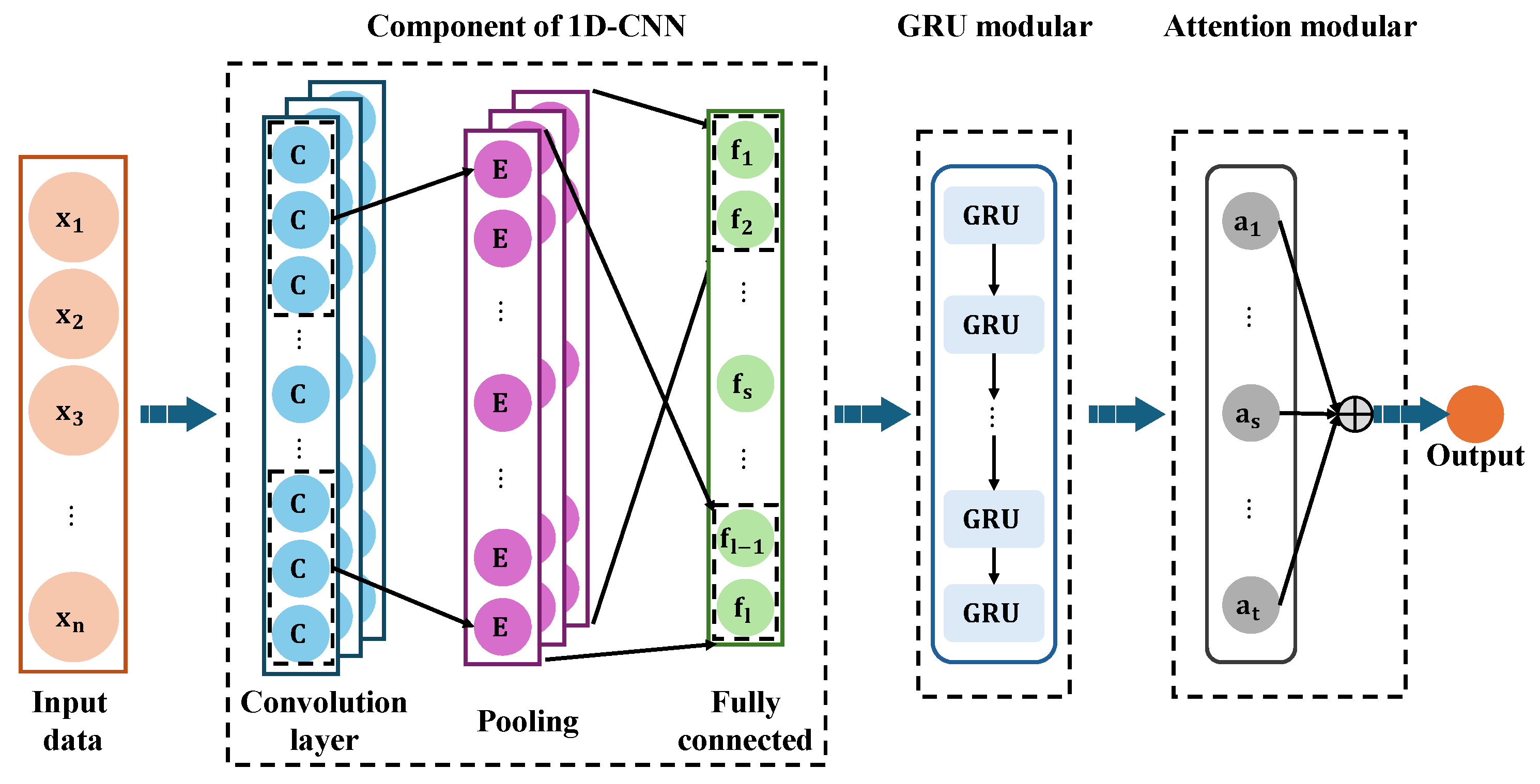
Our proposed CGA-LoadNet is a hybrid neural network architecture that integrates one-dimensional convolution (1D-CNN), gated recurrent units (GRUs), and a self-attention mechanism for short-term electric load forecasting, as shown in Figure 4. This model can simultaneously extract local temporal patterns, capture long-term dependencies, and dynamically emphasize the impact of critical time steps. Given an input load feature sequence, we have the following:

$$\mathbf{X}=[{\mathbf{x}}_1,{\mathbf{x}}_2,\dots ,{\mathbf{x}}_T]\in {\mathbb{R}}^{T\times d},$$

(1)

where T denotes the length of the time series and d denotes the feature dimension. The one-dimensional convolutional neural network first extracts local patterns along the temporal dimension, which can be formulated as follows:

$${\mathbf{H}}_{t,k}^{\left(c\right)}=\sigma \left(\sum _{j=0}^{K-1}{\mathbf{W}}_{k,j}^{\left(c\right)}·{\mathbf{x}}_{t+j}+b_k^{\left(c\right)}\right),k=1,\dots ,C,$$

(2)

where ${\mathbf{H}}^{\left(c\right)}\in {\mathbb{R}}^{T\times C}$ is the convolution output feature map; C is the number of convolution channels (filters); K is the kernel size; ${\mathbf{W}}_{k,j}^{\left(c\right)}$ and $b_k^{\left(c\right)}$ are the convolution kernel weights and biases, respectively; and $\sigma (·)$ is the nonlinear activation function (Sigmoid in this study). This operation enables the model to capture local dependencies and short-term fluctuations in the load sequence.

After the convolutional layer, the output ${\mathbf{H}}^{\left(c\right)}$ is fed into the GRU layer to capture long-term temporal dependencies. The hidden state ${\mathbf{h}}_t$ of the GRU is updated as follows.

$$\begin{array}{cc}{\mathbf{z}}_t\hfill & =\sigma ({\mathbf{W}}_z{\mathbf{h}}_t^{\left(c\right)}+{\mathbf{U}}_z{\mathbf{h}}_{t-1}+{\mathbf{b}}_z)\hfill \end{array}$$

(3)

$$\begin{array}{cc}{\mathbf{r}}_t\hfill & =\sigma ({\mathbf{W}}_r{\mathbf{h}}_t^{\left(c\right)}+{\mathbf{U}}_r{\mathbf{h}}_{t-1}+{\mathbf{b}}_r)\hfill \end{array}$$

(4)

$$\begin{array}{cc}{\tilde{\mathbf{h}}}_t\hfill & =tanh({\mathbf{W}}_h{\mathbf{h}}_t^{\left(c\right)}+{\mathbf{U}}_h({\mathbf{r}}_t\odot {\mathbf{h}}_{t-1})+{\mathbf{b}}_h)\hfill \end{array}$$

(5)

$$\begin{array}{cc}{\mathbf{h}}_t\hfill & =(1-{\mathbf{z}}_t)\odot {\mathbf{h}}_{t-1}+{\mathbf{z}}_t\odot {\tilde{\mathbf{h}}}_t\hfill \end{array}$$

(6)

Here, ${\mathbf{h}}_t\in {\mathbb{R}}^H$ is the hidden state at time t; ${\mathbf{z}}_t$ and ${\mathbf{r}}_t$ are the update and reset gates, respectively; ⊙ denotes the element-wise product; and ${\mathbf{W}}_{*}$, ${\mathbf{U}}_{*}$, ${\mathbf{b}}_{*}$ are the trainable weights and biases. The GRU compresses historical information into hidden states, effectively modeling the long-term dependencies in the load sequence.

To enhance the model’s focus on critical time steps (e.g., peak loads or sudden fluctuations), we introduce a self-attention mechanism over the GRU hidden state sequence, $[{\mathbf{h}}_1,\dots ,{\mathbf{h}}_T]$. The attention weights and the context vector are computed as

$$\begin{array}{cc}{e}_t\hfill & ={\mathbf{v}}^{\top }tanh({\mathbf{W}}_a{\mathbf{h}}_t+{\mathbf{b}}_a)\hfill \end{array}$$

(7)

$$\begin{array}{cc}{\alpha }_t\hfill & ={\displaystyle \frac{exp\left(e_t\right)}{{\sum }_{i=1}^{T}exp\left(e_i\right)}}\hfill \end{array}$$

(8)

$$\begin{array}{cc}\mathbf{c}\hfill & =\sum _{t=1}^T{\alpha }_t{\mathbf{h}}_t.\hfill \end{array}$$

(9)

Here, $e_t$ is the unnormalized attention score at time step t, ${\alpha }_t$ is the normalized attention weight, and $\mathbf{c}\in {\mathbb{R}}^H$ is the context vector obtained through weighted aggregation of the hidden states. The self-attention mechanism adaptively highlights important time steps, thereby improving the model’s sensitivity to load fluctuations and sudden changes.

4. Experiment Evaluation

4.1. Dataset Description and Preprocessing

This study employed publicly available data released by the Australian Energy Market Operator (AEMO) to evaluate the practical applicability and predictive performance of the proposed model. The dataset was obtained from AEMO’s official Weekly Market records (https://data.wa.aemo.com.au, accessed on 30 June 2025). We selected market data covering the period from 6 January 2022, to 5 January 2023, which spans the entire operational cycle of the 2022 calendar year, ensuring good temporal continuity and representativeness. The dataset has a temporal resolution of 30 min intervals, forming a high-resolution electricity load time series suitable for short-term load forecasting tasks.

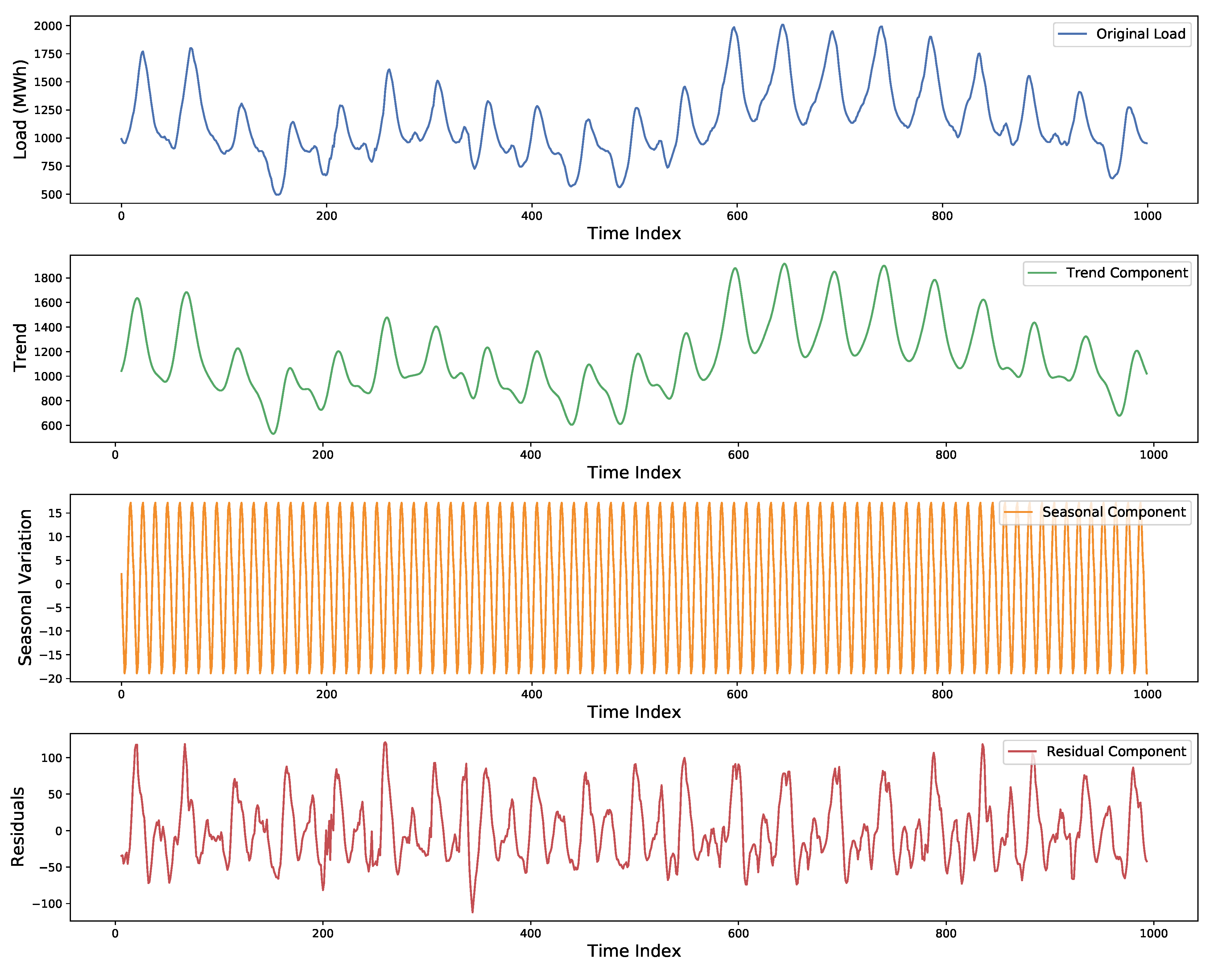
For a deeper understanding of the internal structure of the load sequence, we performed a Seasonal-Trend decomposition using Loess (STL) on the actual load data, as shown in Figure 5. The figure illustrates the original load series along with its decomposed components, long-term trend, seasonal variation, and residual noise. It can be observed that the load data exhibited clear seasonal fluctuations, evolving trend changes over time, and a certain degree of non-stationarity and random disturbance. These characteristics indicate that load forecasting models should simultaneously account for both short-term local patterns and long-term temporal dependencies—an insight that further validates the structural design of our proposed CGA-LoadNet model.

Before training the neural network, a systematic data preprocessing procedure was applied to enhance training stability, efficiency, and convergence. Proper handling of missing data and feature scaling is crucial for achieving stable model performance. First, missing values in the original sequence were imputed using the nearest neighbor method to maintain temporal continuity of the input features. Second, no specific processing was applied to outliers, as neural networks exhibit inherent robustness to occasional anomalies and their occurrence in the dataset was sparse. The preprocessing, therefore, focused primarily on missing-value handling and feature normalization.

Feature scaling was performed to remove the impact of differences in magnitude among variables. All variables were normalized to the range $[0,1]$ using Min-Max normalization. The normalization formula is expressed as

$$X_i={\displaystyle \frac{X_{\mathrm{load}}-X_{min}}{X_{max}-X_{min}}},$$

(10)

where $X_{\mathrm{load}}$ is the original feature value, $X_i$ is the normalized value, and $X_{max}$ and $X_{min}$ represent the maximum and minimum values of the feature, respectively. After model prediction, inverse normalization is applied to recover the original physical units, as shown in the following formula.

$$X_j=(X_{max}-X_{min})·X_i+X_{min},$$

(11)

where $X_j$ denotes the value after inverse normalization.

For sample construction, we adopt a sliding-window approach to transform the time series into a supervised learning format suitable for the model. Specifically, we set the window size to $n_L=24$, meaning that the previous 24 time steps are used as input to predict the load at the next time step. By sliding this window along the sequence, a large number of input–output pairs are generated for training and evaluation of the short-term load forecasting model.

Additionally, the dataset is split chronologically, with the first 80% of the samples used for training and the remaining 20% for validation and testing.

4.2. Problem Description

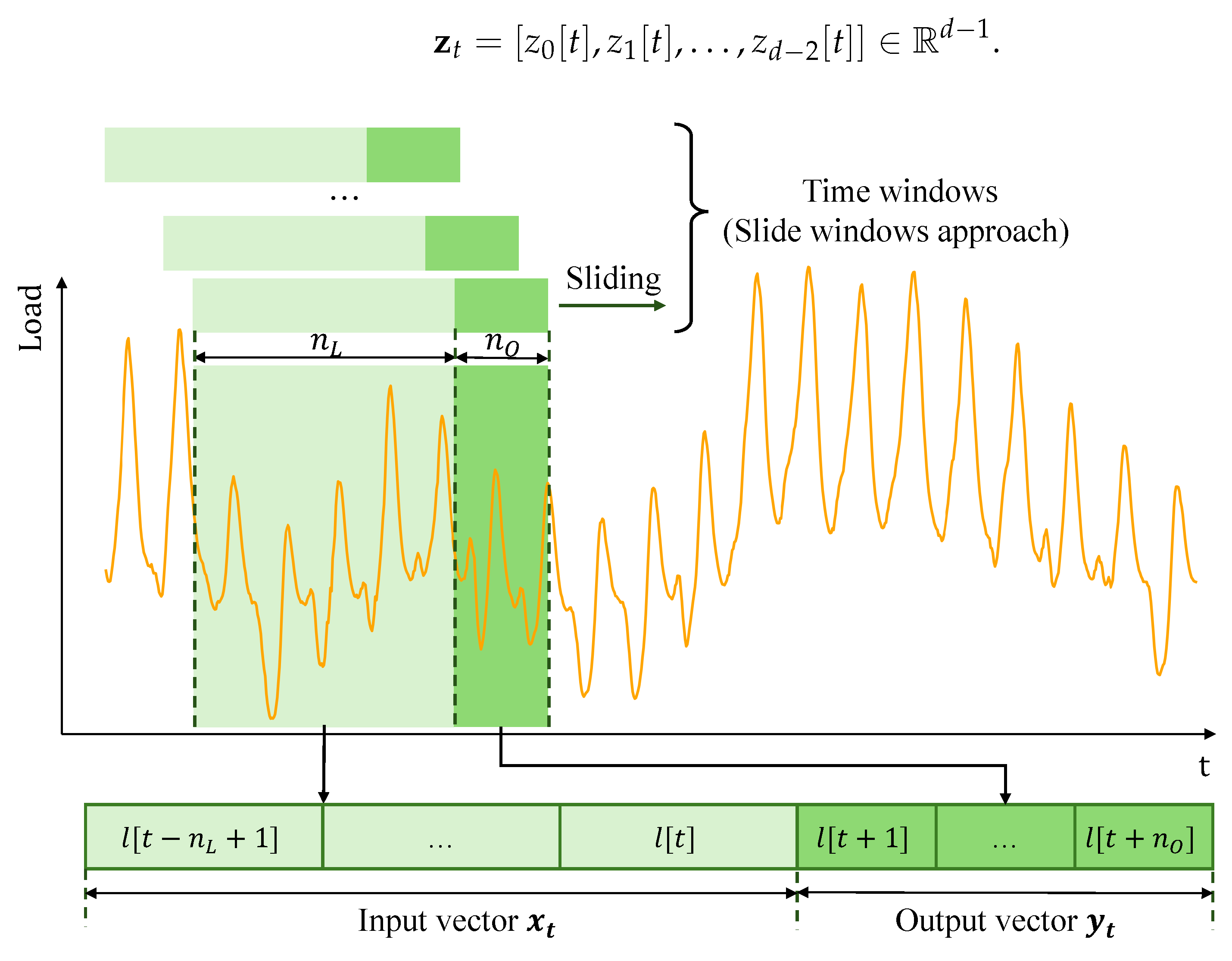
In this study, the electric load forecasting problem is formalized as a supervised learning task. The core idea is to use a sliding time window to divide the time series into multiple input–output pairs, enabling deep learning models to be trained for multi-step prediction. The main concept behind the sliding window approach is to leverage historical load data over a fixed past period to predict future electricity demand over a specified horizon. As illustrated in Figure 6, to more clearly explain the modeling mechanism of the sliding window method, we first introduce the formal definition and symbolic representation of the time series. Let the original electric load time series be denoted as

$$s=\left[s\right[0],s[1],\dots ,s[L\left]\right].$$

(12)

This represents the recorded electric load (e.g., active power) from time $t=0$ to $t=L$. At each time step t, we aim to use the past $n_L$ time steps as input to predict the electric load for the next $n_O$ time steps. Accordingly, we define the input vector (a fixed-length sliding window) as

$${\mathbf{x}}_t=[l[t-n_L+1],l[t-n_L+2],\dots ,l\left[t\right]]\in {\mathbb{R}}^{n_L}.$$

(13)

The output vector corresponds to the electric load values to be predicted over the next $n_O$ time steps.

$${\mathbf{y}}_t=[l[t+1],l[t+2],\dots ,l[t+n_O]]\in {\mathbb{R}}^{n_O}.$$

(14)

By sliding the window over the entire time series, multiple training samples $({\mathbf{x}}_t,{\mathbf{y}}_t)$ can be constructed. In this way, the load forecasting task is transformed into a typical supervised learning modeling task.

In addition to its own historical load $s\left[t\right]$, electric load forecasting can also leverage other external inputs, such as temperature, humidity, and temporal features. Let these external features observed at time t be denoted as

$${\mathbf{z}}_t=[z_0\left[t\right],z_1\left[t\right],\dots ,z_{d-2}\left[t\right]]\in {\mathbb{R}}^{d-1}.$$

When these external features are incorporated, the input becomes a d-dimensional feature vector.

$$\mathbf{x}\left[t\right]\in {\mathbb{R}}^d.$$

This contains the load itself and $d-1$ external features. Specifically, at each time step t, the input vector is defined as

$$\mathbf{x}\left[t\right]=[s\left[t\right],z_0\left[t\right],z_1\left[t\right],\dots ,z_{d-2}\left[t\right]]\in {\mathbb{R}}^d.$$

Accordingly, a complete input window of length $n_L$ (i.e., the number of past steps used for prediction) is given by

$${\mathbf{x}}_t=[\mathbf{x}[t-n_L+1],\dots ,\mathbf{x}\left[t\right]]\in {\mathbb{R}}^{n_L\times d}.$$

4.3. Evaluation Metrics

This study evaluates the predictive performance of the model on the test set using four metrics, $R^2$, RMSE, MAE, and MAPE. Their mathematical definitions are as follows.

$$R^2=1-{\displaystyle \frac{{\sum }_{i=1}^N{(y_i-{\widehat{y}}_i)}^2}{{\sum }_{i=1}^N{(y_i-\overline{y})}^2}},$$

(15)

where $y_i$ denotes the true value (actual load), ${\widehat{y}}_i$ represents the predicted value, $\overline{y}$ is the mean of the true values, and N is the total number of samples. An $R^2$ value closer to 1 indicates that the model can explain a larger proportion of the variance in the target variable.

$$\mathrm{RMSE}=\sqrt{{\displaystyle \frac{1}{N}}{\sum }_{i=1}^N{(y_i-{\widehat{y}}_i)}^2},$$

(16)

where $y_i$ is the true value, ${\widehat{y}}_i$ is the predicted value, and N is the total number of samples. RMSE measures the average deviation between predicted and true values; a smaller RMSE indicates better predictive performance.

$$\mathrm{MAE}={\displaystyle \frac{1}{N}}\sum _{i=1}^N\left|y_i-{\widehat{y}}_i\right|,$$

(17)

where $y_i$ is the true value, ${\widehat{y}}_i$ is the predicted value, and N is the total number of samples. MAE measures the average absolute deviation between predicted and true values, and a smaller MAE indicates higher overall prediction accuracy.

$$\mathrm{MAPE}={\displaystyle \frac{100}{N}}\sum _{i=1}^N\left|{\displaystyle \frac{y_i-{\widehat{y}}_i}{y_i}}\right|,$$

(18)

where $y_i$ is the true value and ${\widehat{y}}_i$ is the predicted value. MAPE expresses the prediction error as a percentage of the true value, which makes it scale-independent and easier to interpret across different datasets. A smaller MAPE indicates that the predictions are, on average, closer to the actual values in relative terms.

These four metrics evaluate the model’s predictive performance from different perspectives: $R^2$ reflects the goodness of fit, RMSE and MAE quantify absolute prediction errors, while MAPE provides an intuitive percentage-based measure of relative error.

4.4. The CGA-LoadNet Approach

In this study, we propose CGA-LoadNet, a hybrid deep learning model designed to capture both local temporal patterns and long-term dependencies in electricity load sequences. The network consists of three main components, a 1D-CNN, a GRU layer, and a self-attention mechanism.

The 1D-CNN layer extracts local features along the temporal dimension, transforming the 19-dimensional input into 24 feature channels. A convolutional kernel size of 1 is employed with zero-padding of one unit on both sides to preserve the sequence length. A Sigmoid activation function is applied to introduce non-linearity. The output is then fed into a GRU layer with 12 hidden units, which models the sequential dependencies in the load time series. An attention mechanism is applied to the GRU outputs to compute dynamic importance weights for each time step, generating a context vector that emphasizes critical periods for prediction. Finally, a fully connected layer maps the context vector to the target load value.

For model training, we use the Adam optimizer with a learning rate of 0.01 and adopt the Smooth L1 loss as the objective function to balance robustness and precision. The model is trained for 100 epochs with a batch size of 128.

5. Result Analysis

This section presents a comprehensive analysis of the predictive performance of each model using tables, line charts, and evaluation metrics. Specifically, we focus on prediction accuracy and error distribution, and we quantify the effectiveness of the proposed CGA-LoadNet method based on key metrics, such as $R^2$, RMSE, MAE, and MAPE.

First, we compare the predicted power load curves with the actual load curves on the test set to visually assess the performance differences among the models. As shown in Figure 7a,b, the predicted power load results are presented for two time intervals, from 2:00 to 14:00 on 24 October and from 2:00 on 24 October to 14:00 on 25 October. During periods with significant load fluctuations, the predicted curve of CGA-LoadNet aligns more closely with the actual load trajectory, while other baseline models exhibit varying degrees of deviation, particularly during peak hours or sudden changes.

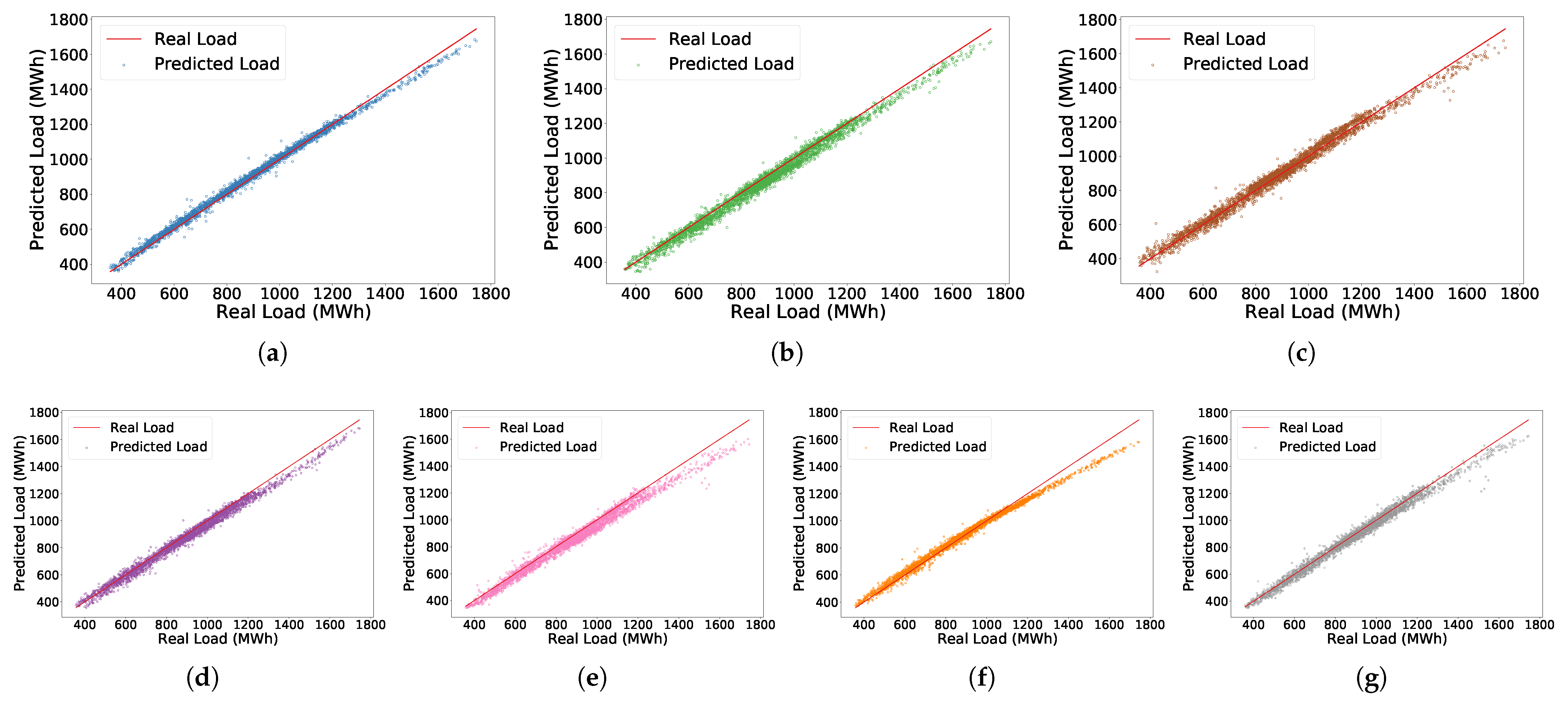
To further assess the overall prediction accuracy of each model, we plotted the predicted values against the actual values in diagonal plots, as shown in Figure 8a–g. The figure contains seven subplots, corresponding to six baseline models and the proposed CGA-LoadNet. In each plot, the x-axis represents the actual load values, while the y-axis indicates the predicted values. The red solid line denotes the ideal diagonal, representing perfect prediction. The prediction points of CGA-LoadNet are more densely concentrated around the ideal diagonal, while the baselines show greater deviations, particularly in high-load regions.

Subsequently, we compared the relative error distributions of the different models on the test set. As shown in Figure 9, the violin plot illustrates the probability density and dispersion of tthe prediction errors. The error distribution of CGA-LoadNet was the most concentrated, with a narrow spread around zero and minimal fluctuation range. By contrast, the baseline methods displayed wider violin shapes and more dispersed distributions, reflecting larger variability in their errors.

Finally,

Table 2. Evaluation metrics ($R^2$, RMSE, MAE, and MAPE) for electricity load forecasting.

Comparison Methods	${\mathit{R}}^2$ Score	RMSE Score	MAE Score	MAPE Score
RNN	0.981	31.47	24.24	2.89
LSTM	0.979	33.49	25.74	2.94
GRU	0.982	30.36	21.23	2.38
Conv1D_RNN	0.985	27.55	22.78	2.61
Conv1D_LSTM	0.963	44.10	33.63	3.80
Conv1D_GRU	0.981	31.48	23.43	2.70
CGA-LoadNet (Ours)	0.993	18.44	13.94	1.72

summarizes the performance of all the models on the test set in terms of $R^2$, RMSE, MAE, and MAPE. The proposed CGA-LoadNet achieves the highest $R^2$ score of 0.993 and records the lowest error values across the three error metrics, with an RMSE of 18.44, an MAE of 13.94, and a MAPE of 1.72, whereas other models show larger gaps in accuracy and stability. These findings clearly demonstrate the superior predictive performance of CGA-LoadNet, and the subsequent discussion provides a detailed interpretation of these results.

6. Conclusions

This paper introduces CGA-LoadNet, a hybrid deep neural network model that integrates a 1D-CNN, GRUs, and a self-attention mechanism for short-term electricity load forecasting. The design leverages convolutional layers for local temporal feature extraction, GRU for modeling long-term dependencies, and self-attention for adaptively focusing on critical time steps. Experimental results demonstrate that CGA-LoadNet consistently outperforms baseline methods, including RNN, LSTM, GRU, and their convolutional variants. The model achieves an $R^2$ score of 0.993, while the error metrics reach values of 18.44 for RMSE, 13.94 for MAE, and 1.72 for MAPE. These results confirm significant improvements in accuracy and stability compared with the other models.

Nevertheless, several limitations should be acknowledged. First, the current study mainly addresses short-term forecasting, and the model’s capability for medium- and long-term horizons has not yet been fully validated. Second, the method relies on sufficient amounts of high-quality historical data, which may restrict its applicability in data-scarce or noisy environments. Finally, important exogenous variables, such as weather conditions, socio-economic indicators, and special events, were not explicitly incorporated, which could limit predictive accuracy under highly dynamic scenarios.

Future work will extend the model to medium- and long-term forecasting tasks, incorporate exogenous variables such as weather and economic indicators, as well as enhance interpretability through attention weight visualization and feature contribution analysis. These directions will improve robustness, transparency, and practical applicability in smart grid operations.

In conclusion, despite these limitations, the proposed CGA-LoadNet provides an efficient, accurate, and practically viable solution for short-term electric load forecasting, with strong potential for deployment in modern power system scenarios.

References

- Adham, M.; Keene, S.; Bass, R.B. Distributed Energy Resources: A Systematic Literature Review. Energy Rep. 2025, 13, 1980–1999. [Google Scholar] [CrossRef]
- Judge, M.A.; Khan, A.; Manzoor, A.; Khattak, H.A. Overview of smart grid implementation: Frameworks, impact, performance and challenges. J. Energy Storage 2022, 49, 104056. [Google Scholar] [CrossRef]
- Hu, Y.; Li, J.; Hong, M.; Ren, J.; Man, Y. Industrial artificial intelligence based energy management system: Integrated framework for electricity load forecasting and fault prediction. Energy 2022, 244, 123195. [Google Scholar] [CrossRef]
- Singh, A.R.; Sujatha, M.; Kadu, A.D.; Bajaj, M.; Addis, H.K.; Sarada, K. A deep learning and IoT-driven framework for real-time adaptive resource allocation and grid optimization in smart energy systems. Sci. Rep. 2025, 15, 19309. [Google Scholar] [CrossRef] [PubMed]
- Alam, M.M.; Hossain, M.; Habib, M.A.; Arafat, M.; Hannan, M. Artificial intelligence integrated grid systems: Technologies, potential frameworks, challenges, and research directions. Renew. Sustain. Energy Rev. 2025, 211, 115251. [Google Scholar] [CrossRef]
- Abrahamsen, F.E.; Ai, Y.; Cheffena, M. Communication technologies for smart grid: A comprehensive survey. Sensors 2021, 21, 8087. [Google Scholar] [CrossRef]
- Wang, F.; Nishter, Z. Real-time load forecasting and adaptive control in smart grids using a hybrid neuro-fuzzy approach. Energies 2024, 17, 2539. [Google Scholar] [CrossRef]
- Rajaperumal, T.; Columbus, C.C. Transforming the electrical grid: The role of AI in advancing smart, sustainable, and secure energy systems. Energy Inform. 2025, 8, 51. [Google Scholar]
- Hachache, R.; Labrahmi, M.; Grilo, A.; Chaoub, A.; Bennani, R.; Tamtaoui, A.; Lakssir, B. Energy Load Forecasting Techniques in Smart Grids: A Cross-Country Comparative Analysis. Energies 2024, 17, 2251. [Google Scholar] [CrossRef]
- Zhang, D.; Xu, Y.; Li, Y. Electric load forecasting based on kernel extreme learning machine optimized by improved sparrow search algorithm. Sci. Rep. 2025, 15, 22273. [Google Scholar] [CrossRef]
- Ugbehe, P.O.; Diemuodeke, O.E.; Aikhuele, D.O. Electricity demand forecasting methodologies and applications: A review. Sustain. Energy Res. 2025, 12, 19. [Google Scholar] [CrossRef]
- Raffoul, E.; Tuo, M.; Zhao, C.; Zhao, T.; Ling, M.; Li, X. Comparative Analysis of Machine Learning Models for Short-Term Distribution System Load Forecasting. arXiv 2024, arXiv:2411.16118. [Google Scholar] [CrossRef]
- Hasanat, S.M.; Ullah, K.; Yousaf, H.; Munir, K.; Abid, S.; Bokhari, S.A.S.; Aziz, M.M.; Naqvi, S.F.M.; Ullah, Z. Enhancing short-term load forecasting with a CNN-GRU hybrid model: A comparative analysis. IEEE Access 2024, 12, 184132–184141. [Google Scholar] [CrossRef]
- Kong, X.; Chen, Z.; Liu, W.; Ning, K.; Zhang, L.; Muhammad Marier, S.; Liu, Y.; Chen, Y.; Xia, F. Deep learning for time series forecasting: A survey. Int. J. Mach. Learn. Cybern. 2025, 16, 5079–5112. [Google Scholar] [CrossRef]
- Yazici, I.; Beyca, O.F.; Delen, D. Deep-learning-based short-term electricity load forecasting: A real case application. Eng. Appl. Artif. Intell. 2022, 109, 104645. [Google Scholar]
- Xue, S.; Huang, H.; Liu, J.; Yang, Q.; Zhao, L.; Wu, H. An Effective Scheme to Solve Critical Data Missing Problems for IoT-Based Smart Energy Management. IEEE Internet Things J. 2024, 12, 4466–4474. [Google Scholar] [CrossRef]
- Wang, C.; Wang, Y.; Ding, Z.; Zheng, T.; Hu, J.; Zhang, K. A transformer-based method of multienergy load forecasting in integrated energy system. IEEE Trans. Smart Grid 2022, 13, 2703–2714. [Google Scholar] [CrossRef]
- Huang, Z.; Yi, Y. Short-Term Load Forecasting for Regional Smart Energy Systems Based on Two-Stage Feature Extraction and Hybrid Inverted Transformer. Sustainability 2024, 16, 7613. [Google Scholar] [CrossRef]
- Lu, Y.; Wang, G.; Huang, X.; Huang, S.; Wu, M. Probabilistic load forecasting based on quantile regression parallel CNN and BiGRU networks. Appl. Intell. 2024, 54, 7439–7460. [Google Scholar] [CrossRef]
- Kim, T.Y.; Cho, S.B. Predicting residential energy consumption using CNN-LSTM neural networks. Energy 2019, 182, 72–81. [Google Scholar] [CrossRef]
- Abbas, M.; Che, Y.; Maqsood, S.; Yousaf, M.Z.; Abdullah, M.; Khan, W.; Khalid, S.; Bajaj, M.; Shabaz, M. Self-adaptive evolutionary neural networks for high-precision short-term electric load forecasting. Sci. Rep. 2025, 15, 21674. [Google Scholar] [CrossRef] [PubMed]
- Wen, X.; Liao, J.; Niu, Q.; Shen, N.; Bao, Y. Deep learning-driven hybrid model for short-term load forecasting and smart grid information management. Sci. Rep. 2024, 14, 13720. [Google Scholar] [CrossRef] [PubMed]