Abstract
We investigate two closely related Lattice Gas Cellular Automata models of the interplay of aggregation of biological cells and synchronization of intracellular oscillations (“clocks”): clock-dependent aggregation, where the adhesive forces between cells depend on their relative clock phases (akin to so-called “swarmalators”), and simple adhesive aggregation, where they do not. Patterns of aggregation are similar for comparable ranges of parameters. However, while simple adhesive aggregation is quite similar to perikinetic aggregation, we show that clock-dependent aggregation differs in subtle ways. We found that it tends to inhibit coalescence of patterns and regularizes aggregate shapes, and, unintuitively, tends to enhance overall synchronization of clocks. Specifically, clock-dependent aggregation showed higher average circularity of aggregates and a larger value of Kuramoto’s r, measuring synchrony. Our results add to the growing literature on swarmalator models and give additional theoretical backing to the previously proposed idea that intracellular oscillatory processes may serve to regularize pattern formation, e.g., in chondrogenic condensation in embryonic chicken limbs. They thus contribute to a partial answer to the question: In the feedback between clocks and attraction in swarmalator models, how important is the effect of clocks on attraction? The detailed, systematic comparison of the results of these two types of aggregation is novel.
Keywords:
swarmalators; synchronization; cell aggregation; pattern formation; Lattice-Gas Cellular Automata MSC:
92B25; 37B15; 92C15
1. Introduction
1.1. Overview
Cellular aggregation is a common phenomenon in biology, e.g., in development, for instance, in the condensation of precartilage cells in developing limbs, see, e.g., [1], and in aggregative organisms on the threshold of multicellularity [2]. There is a plethora of different mechanisms that are responsible for these aggregative processes, for instance, chemotaxis [3] or the coordination of turning rates [4,5].
In this paper, we are interested in possibly the simplest form of cellular aggregation, the formation of cell aggregates via cell–cell adhesion on non-adhesive substrates. This has been experimentally and theoretically investigated as a model of the formation of cancer tumors [6,7,8]. In [7], the authors investigated the dynamics of the aggregation of murine sarcoma cells transfected to express the cell–cell adhesion molecules E-cadherins. Once deposited in vitro on the substrate, they form aggregates which grow in size, and correspondingly decrease in numbers [7]. Once formed, these aggregates undergo compaction: Clusters round up, compact, and, by growing in the third dimension, become spherical. The authors showed that this process of self-assembly is analogous to the well-studied phenomenon of perikinetic aggregation of diffusive colloidal particles first studied by Smoluchowski [9]. As such, this process is an example of diffusion limited aggregation [10]. This mechanism is analogous to what we refer to as simple adhesive aggregation. Various simple mathematical models of this process have been proposed and investigated by these and other authors [6,7,8].
Aggregation of cells is, in some cases, accompanied by the simultaneous synchronization of intracellular oscillatory processes, for example, the cyclical production of the chemotactic agent cyclic adenosine monophosphate (cAMP) in the slime mold Dictyostelium discoideum [3], or the synchronization of the periodic reversal of directions controlled by intracellular oscillations of the “frizzy” (Frz) system and mutual gliding motility proteins (MglAB) in myxobacteria [11,12]. While these two model organisms have been studied extensively, there has been relatively little study of the general mechanisms of the interplay of aggregation and synchronization.
The work at hand is adding to the growing literature of so-called “swarmalator”-type models (swarming oscillators); i.e., models in which synchronization and aggregation of particles is linked. As such, we are not modeling a specific biological phenomenon, but rather a general class of mathematical models that describes a general phenomenon [13,14,15,16]. Specifically, we address the question of how the oscillations in swarmalator-type behavior influence aggregation by conducting an in-depth quantitative analysis of the differences between the aggregation patterns with and without phase-dependent adhesion. This comparison is novel.
1.2. Previous Work on Aggregation and Synchronization
Tanaka and coworkers studied aggregation in systems of chemotactic oscillators [17,18]. In a seminal series of papers, O’Keeffe et al. investigated a model swarming oscillators (“swarmalators”) [14,15,16]. In the swarmalator model, particles have internal oscillators (“clocks”) that interact with each other in a Kuramoto model-like fashion and attract each other, where this attraction is clock-phase-dependent. So two swarmalators that have the same clock phase attract each other stronger than swarmalators in opposite clock phases. This attraction is global, i.e., the force of attraction is independent of the distance of the swarmalators. In [19], we set up and studied a related model of intracellular oscillators with phase-dependent adhesion. Adhesion is of course a local property, meaning that in contrast to O’Keeffe et al.’s swarmalator model, here attraction is local, not global. A partial differential equations model incorporating the Kuramoto model [20,21] and the Armstrong model of cell–cell adhesion [22] was set up and its pattern formation abilities were analyzed via linear stability theory and numerically by Glimm and Gruszka in [19], showing a range of possible patterns in space and clock synchronization. A variant was also investigated via the Cellular Potts Model by Una and Glimm [23], which allows for effects like size and shape fluctuations, since cells are modeled as spatially extended entities instead of modeling cells only as point particles or via their density.
In these models, neighbors seek to synchronize their clocks. When cells do not adhere to each other at all, or when cells in the same clock phase repulse each other, this leads to global synchronization without spatial aggregation. More interesting is the case where cells adhere to each other. In this case, spatial cell clusters form, within which cells’ clocks are synchronized. However, different aggregates are typically synchronized to different clock phases; see Figure 1 for more details.
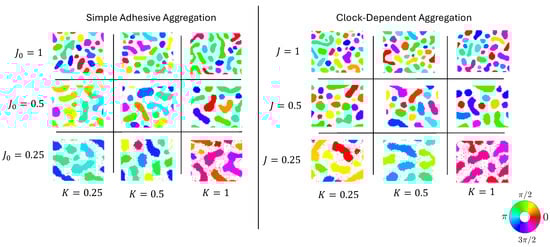
Figure 1.
Parameter sweeps of simulations of simple adhesive aggregation (left) and clock-dependent aggregation (right). States after 2000 simulation steps with identical random initial conditions and 6000 particles ( particle density). Clock phases are shown via colors; see the inlayed color wheel.
Such clusters form without differential adhesion as well, i.e., if the adhesion strength between two cells is independent of their clock phases. This, then, raises the natural question of how the two processes differ: on the one hand, aggregation and synchronization with clock-dependent adhesion (cells in the same phase adhere particularly strongly), and on the other hand, simple (clock-independent) adhesive aggregation.
1.3. Our Model and Results
In the paper at hand, we investigate the question above by comparing two slightly different models as a follow-up of a model in our paper [19]: simple adhesive aggregation is the case in which the base clock-independent adherence strength (denoted by in our model) is positive and the clock-dependent differential adhesion strength (denoted by J) is zero; for clock-dependent aggregation, this is reversed.
Our results shed light on the behavior of swarmalator-type models, specifically in the parameter domain, where cells aggregate into clusters while simultaneously undergoing synchronization. The feedback of synchronization and aggregation (clock-dependent aggregation) improves synchronization and leads to smaller and more compactly shaped clusters compared to the case where synchronization and aggregation are completely separate processes (simple adhesive aggregation); see Section 3.
For an application more closely related to a specific biological phenomenon, the results give additional theoretical backing to the idea that internal oscillatory processes may serve to “regularize” patterns in aggregative pattern formation. This idea was first discussed by Bhat et al. [24]; see also [25]. Bhat et al. argue that the inclusion of intracellular Hes1 oscillations regularizes the patterns of chondrogenic condensations (cellular aggregates) in chick embryos in in vitro experiments; i.e., it makes condensations more uniform and more clearly demarked. They show that if the effect of such synchronous oscillations is added their model of chondrogenesis [26], this is indeed the case. The authors of [24] used a partial differential equations model with externally imposed synchrony of such oscillations; i.e., they are not the outcome of model-inherent oscillation dynamics as in our model. In one crucial aspect their model is similar to the model in this paper though: in both cases, cell–cell adhesion depends on relative clock phases.
2. Model Description
2.1. Overview
We use the model we proposed in [19]. In it, individual cells are represented by points that move according to certain probabilistic rules. Before giving the details below, we note that the idea is that aggregation is modeled via the fact that two cells are more likely to move towards each other than away from each other. These probabilities are influenced by the states of the two internal cell clocks.
Specifically, our Lattice Gas Cellular Automaton (LGCA) model is based on models of cell–cell adhesion and aggregation; see Figure 2 and [19,27,28] for more information. The model is using a 2-dimensional hexagonal lattice with periodic boundary conditions. Each hexagonal node has six “channels,” one for each edge. Each channel corresponds to a direction of motion. Each of the six channels in a hexagon can either be occupied by one particle or unoccupied. So there are between zero and six particles in a hexagon at a given time, all in different channels. Additionally, each particle has a clock associated with it. The “state” of a node is the collection of occupied channels in it with corresponding clock values, i.e., collections , where is the occupancy number (0 or 1) of the ith channel, and corresponding clock values .
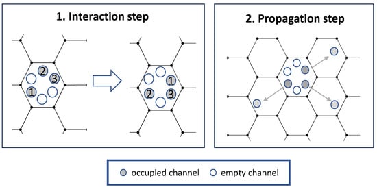
Figure 2.
Schematics for the Lattice Gas Cellular Automaton model. Adpated from [19].
The key idea of the model is that spatiotemporal evolution is modeled via two steps: an interaction step and a propagation step; see Figure 2 for more information. In the propagation step, cells move from one node to a neighboring one in the direction given by their channel. In the interaction step, the state of each node is updated. For this, each possible rearrangement of the particles in a node (state with clock values ) is assigned an energy . A new state is then chosen with probability
where Z is a constant chosen such that the sum of all the probabilities is unity. Note that the more positive the energy is, the higher is the probability that the state is chosen. In our case, is calculated by considering how each particle interacts with the neighboring particles. Specifically,
Here is the vector of direction corresponding to channel i, and is a vector in the direction of a (first-order) neighbor’s lattice site. (See Figure 3). The clock values of the particle in channel i and the neighbor are and , respectively.
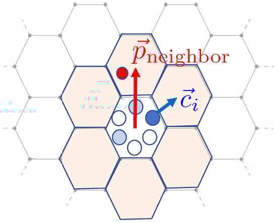
Figure 3.
Schematics for computing the transition probabilities in the interaction step. The formalism means that new channel directions tend to be aligned with the neighbor’s location vector , modeling cell–cell adhesion. See the text for more details. Adpated from [19].
To understand how adhesion and repulsion are modeled, consider the energy (2). Note that if the vectors and are pointed in the same direction, their dot product is positive. Thus, assuming for now that the additional factor is positive as well, this means the direction of motion of a cell is biased towards this neighbor. This models cell–cell adhesion. The baseline adhesion strength is encompassed in , and there is an additional adhesion term that is dependent on the difference in clock values between a cell and its neighbor. Its strength is denoted by J.
Let us discuss the influence of the factor in the energy (2). The case means that all the states have equal energy , and so the transition probabilities (1) are all equal. Thus, this corresponds to unbiased random movement (diffusion). For positive , we get attraction between neighboring cells. For positive J, the term is positive for cells with similar clock phases (). This means that such cells adhere to each other. In contrast, cells with opposite clock phases () actually repulse each other. The form of these equations is motivated by the swarmalator model of O’Keeffe et al. [15], but with local instead of global interactions. For this paper we only used positive and J.
Finally, the clocks are updated based on a discrete Kuramoto-type model [20]. For this, every LGCA step is subdivided into n subintervals of length . (In simulations, we used .) In each subinterval, the change in clock value of the particle at channel i is given by the finite-difference approximation of the Kuramoto model
Here the sum is over the first-order neighbors of the particle in channel i and the particles in the other channels of the same hexagonal node (total particles). The coupling strength of the oscillators is denoted by K. For this work, we focused on . That means that particles want to synchronize with their neighbors. We can assume without loss of generality that by shifting the frame in the clock phase by the term , where t is the number of time steps.
2.2. Implementation and Analysis
In this paper we are focusing on the roles of and J in the model. That is, we are aiming to understand the difference between a baseline adhesion and an adhesion that is dependent on the clock values. To achieve this we ran a set of simulations with and (clock-dependent aggregation) and another set with and (simple adhesive aggregation) for some positive a. The rest of the parameters were identical for both the simulations. Then we looked at four parameters to make conclusions: average radius of gyration of the aggregates (), average circularity of the aggregates (C), the number of aggregates in the simulation (n), and how synchronized the aggregates are (r).
We implemented the LGCA model in the programming language MATLAB R2024a with 6000 particles on hexagonal lattice. In each simulation step, each of the particles’ channels was updated according to the probabilistic rules described in Section 2.1 (interaction step), and then each position was updated according to the propagation step. See the data availability statement of this paper for a link to the code. The simulations were run on a standard PC with 64 GB RAM and an Intel Core i7-1370P 1.90 GHz processor.
Counting aggregates: To count aggregations, we employed two different techniques. For the “total count”, we first plotted all the cells with disk-shaped points. The radius of these disks was chosen so that cells in adjacent channels in one hexagon overlapped, and cells in adjacent hexagons in channels that shared a joint edges also overlapped. We then used the Matlab routine bwconncomp to count the number of connected components. We joined up 91 copies of the simulation domain to create one big picture with periodically repeating images arranged in a hexagonal shape. This is possible because of the periodic boundary conditions. We then determined the number of cells as 1/91th of the number of connected components in this big picture. See the Supplementary Figure S1 for an illustration. In a second method we refer to as “cleaned count”, we first removed any cell that is in a hexagonal node that has two or less cells in it. This helps smooth the boundaries of the aggregates and remove any straggler particles later in the aggregation process.
Radius of gyration and circularity: To calculate the average radius of gyration of clusters, we used MATLAB’s bwconncomp to identify the pixels of the connected components (aggregates) from the images generated for the “cleaned count”. Then the radius of gyration for a single aggregate was calculated by
Here M is the number of pixels in the aggregate, is the pixel location, and is the location of the aggregate’s centroid. We used MATLAB’s regionprops function to get the centroids of the aggregates. The same function was also used to find the mean (bias corrected) circularity of aggregates. The circularity c of a cluster is defined as the ratio of times its area and the square of its perimeter. By the isoperimetric inequality, c lies between 0 and 1, with corresponding to a perfect disk. There is an additional factor for bias correction that corrects issues with small clusters, where the discretization may lead to circularities greater than 1; see [29].
Kuramoto’s r: A standard measure of synchronization is Kuramoto’s order parameter r [20]. Given n clock values where , it is defined via
Note that . In the completely synchronized case (), we have . Values of r close to zero indicate completely unsynchronized (“incoherent”) behavior. We computed Kuramoto’s r numerically using the clock phase value of the cells.
Dependence of Kuramoto’s r on number of oscillators: As stated above, in the case of large n with clock values being uniformly distributed over the interval we have . This is the incoherent case where the clock values are completely randomly distributed without even partial synchronization. But due to finite-size effects (finite n), the value of is not exactly zero. To investigate this situation in more depth, we considered the simple model of finite n and we chose values randomly. As shown below, the expected value of is not exactly zero, but decays as ; see Corollary 1 for more information. [This is a simple result that is likely known, but we have not found previous mention in the literature. We have, therefore, included a formal proof here.] In fact, we have the following result:
Theorem 1.
Consider a random variable defined as follows: Choose first a random positive integer N with some probability density function . Then choose independently from with the uniform distribution. Let . Then the expected value of X is .
Proof.
This is a straightforward computation:
In the second row, we used the relation
□
In particular, we have the following Corollary:
Corollary 1.
Let n be an integer and a collection of independent, uniformly distributed random variables from . Then the expected value of Kuramoto’s parameter defined in (5) is .
For our simulations, we sought to investigate the question of whether the observed partial synchronization where each cluster is synchronized to a different clock phase is analogous to the simple model of randomly chosen clock values investigated above. To do so, we computed the index , where n is the number of clusters (counted with the “cleaned count” method). By Theorem 1, values of close to 1 indicate that the distribution of cluster clock values is essentially random. We used this in Section 3 to analyze our synthetic data; see there for further discussion.
3. Quantitative Results
3.1. Parameter Sweep
We conducted two types of simulations: simple adhesive aggregation, characterized by clock-independent adhesion (), and clock-dependent aggregation (). Figure 1 shows a comparison of the typical results for different values of the adhesion strength J or and the clock coupling rate K. For any combination of parameters, aggregation of clusters was observable, where the number of clusters and their shape depended on the parameters. The clock phases were synchronized within clusters. For the maximum clock coupling rate and minimum adhesion strength, all the cluster clock phases were almost the same for all clusters (“global synchronization”); for all the other values, different clusters were synchronized to different clock values (“local synchronization”).
Note that for fully synchronized particles, the adhesion strength for the two models is the same if the values of J and are the same. For this reason, differences in cluster number, shape, and synchronization were subtle. It is noticeable though that clock-dependent aggregation yielded larger numbers of clusters for comparable parameters. In the following, we will investigate these subtle differences between the two models in more depth. To focus on these differences, and because each simulation run took several hours, we concentrated our simulations on the parameters and and quantifed their differences in a number of different ways.
3.2. Number of Aggregates
As cells in our model undergo random walks and adhesion, they form cluster, or aggregates. As seen in Figure 4, these aggregates grow in size, and their number decreases, from initially about 1700 to around 100 within 40 time steps.
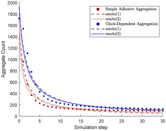
Figure 4.
Number of aggregates as a function of simulation time steps (“total count” algorithm). Data point are based on mean values for simulations. Also shown are weighted least squares best fits for the models smolu(1) and smolu(2) as discussed in the text.
Figure 4 shows the number of aggregates as a function of time steps. We compared the two cases of simple adhesive aggregation and clock-dependent aggregation. Aggregation is slower in the case of clock-dependent aggregation, resulting in significantly larger number of aggregates.
For further analysis, we used the Smoluchowski model [9] to analyze to what extent the data fits the results of a perikinetic process. (As recognized already by others [6,7,8], this analogy is only true in the initial phase of cluster formation, at least under the assumption that the rate constant of collision of clusters does not depend on the size of the clusters. We, therefore, only used the data for the first 40 out of 200 time steps.)
Denote by the number of aggregates of size k, and by the (constant) aggregation rate between clusters of size i and j. Smoluchowski’s equations are then
The total number of clusters at time t is then . We considered two scenarios, which we denote by smolu(1) and smolu(2):
- smolu(1)We assumed for all , i.e., the aggregation rates are independent of the sizes of the clusters; we denoted this rate by . This leads to the equation , which has the solutionNote this model has two parameters: The constant aggregation rate and the initial number of aggregates .
- smolu(2)As a slightly more complex model, we assumed that the aggregation rate is constant for clusters of size greater than 1, but different for the aggregation rate involving clusters of size 1. In short, we had two rates given byThis gave rise to the following coupled system:Note that this simplifies to the previous model for . Solutions to this model have no readily available closed form, but the system can be solved numerically. There were four parameters: Besides the rates and , we had the initial conditions and , the total numbers of clusters and the number of clusters of size 1, respectively.
We performed weighted least squares curve fitting for the data, which consists of the aggregate count at each time step, averaged over 40 simulations. The fitted parameters were and for smolu(1) and and for smolu(2). The weights were the inverse variances of the data each time step to account for size effects, also known as (nonlinear) inverse variance weighted least squares regression, a common approach when fitting data that consists of time series of averages with distinct standard deviations at each point in time, see, e.g., [30]. The results were as followed (also see Figure 4):
- Simple adhesive aggregation, smolu(1): , .
- Simple adhesive aggregation, smolu(2): , ,.
- Clock-dependent aggregation, smolu(1): , .
- Clock-dependent aggregation, smolu(2): , , .
Note that the models fit somewhat better for simple adhesive aggregation, where smolu(2) is a slight improvement over smolu(1) with an aggregation rate for size 1 particles that is about twice as large as the aggregation rate for larger particles . The optimal fit also yielded , i.e., initially, all clusters are of the minimum size. These are plausible results since diffusivity decreases with aggregate size, and also, our random initialization yielded an initial distribution where most clusters only occupied one hexagon. For clock-dependent aggregation, both outcomes are reversed, remarkably, with the aggregation rate for the smallest aggregates being many orders of magnitude smaller than the aggregation rate for larger particles and very few particles being of the smallest size initially—clearly an unrealistic results.
The fitting suggests that the two aggregation processes, while yielding seemingly quite similar results on a superficial level, give rise to quite distinct dynamics at closer look.
3.3. Compaction
One of the key findings of the experimental study of the experimental adhesive aggregation study of sarcoma cells in [7] was that forming aggregates were also simultaneously undergoing compaction: clusters rounded up, compacted, and, by growing in the third dimension, became spherical. In our two-dimensional model, we cannot account for this effect directly. However, we have found that a similar effect occurs in that clusters that were initially irregularly shaped rounded up with time and became more disk-like.
To investigate this numerically, we considered two measurements: the average circularity of clusters and the average radius of gyration. (See section on Model Implementation above.) The circularity index measures the typical “roundness” of clusters with a number between 0 and 1, with 1 corresponding to a perfect disk. The radius of gyration of a cluster of points can be interpreted as an average distance to its center of mass; for a fixed number of points, a disk has minimum radius of gyration. (See also [8]).
Figure 5 shows the averaged results of the simulations of the two indices. The circularity index is close to one initially in both models due to small clusters, which are well approximated by disks. As the cells aggregate, clusters form in irregular shapes, leading to a rapid decrease in circularity. After this initial formation phase, coalescence of the clusters slows down and the clusters slowly round up, leading to an increase in circularity. In contrast, the radius of gyration shows a monotonic increase—this reflects the fact that the average area of clusters continues to increase due to coalescence.
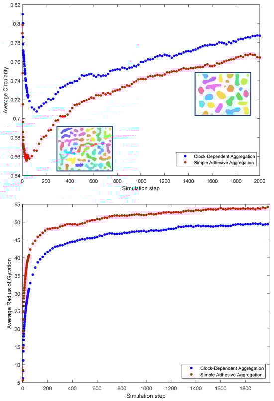
Figure 5.
Measures of compaction: average circularity (top) and average radius of gyration (bottom) as a function of time (simulation step). Both are based on simulations. Inlaid are images of typical aggregation stages showing the gradual “rounding up” of clusters. (Colors in the inlaid images correspond to phases as in Figure 1).
Note that average circularity is larger throughout aggregation for the clock-dependent aggregation than for the simple adhesive aggregation, with a much less steep initial drop. This indicates that cluster tend to be much rounder and regular for the clock-dependent aggregation throughout the whole process.
3.4. Measures of Synchronization
As aggregates from, clocks synchronize within clusters. But to what extend are clusters synchronized among each other? This can be quantified with Kuramoto’s r parameter. The results of the simulations are summarized in Figure 6. The top panel shows the average value of Kuramoto’s r as a function of time step. Note that the value is higher for the clock-dependent aggregation model than for the simple adhesion aggregation, indicating a larger degree of synchrony in this case. This is a somewhat surprising result, given that there tends to be a larger number of clusters in clock-dependent aggregation, all synchronized to different clock phases. If the clock phases were assigned purely by chance, one would expect a lower r-value instead.
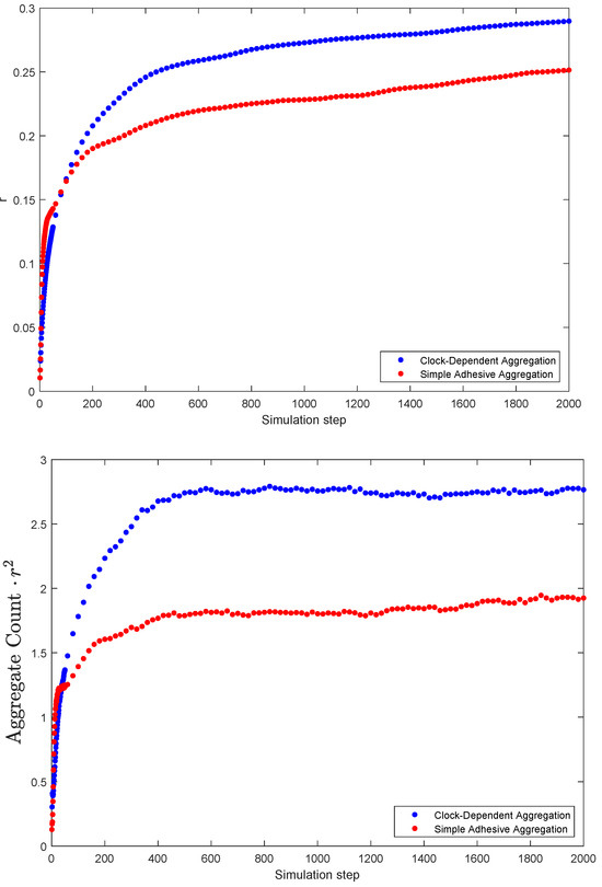
Figure 6.
Measures of synchrony: Kuramoto’s r parameter (top) and the product of number of clusters and Kuramot’s r squared (bottom) as a function of time (simulation step). Both are based on simulations. (The number of clusters n is based on the “cleaned count” algorithm, see Section 2.2).
To investigate this in more depth, we considered the following question: if we have n synchronized clusters, how well can we model the simulation results by simply choosing a random clock value for each cluster? If this was a perfect model, we would expect the mean value over many simulations of to be 1. If this value is larger than 1, we have more synchrony than expected; for long term averages less than 1, we have less synchrony than expected from randomness. We, thus, used the value in our simulations as a measure for how close the situation at hand is to randomly choosing clock values.
Figure 6 shows that for both the simple adhesive aggregation and clock-dependent aggregation, the value is larger than 1, indicating a more-than-random level of synchrony. But here again one sees that this effect is considerably stronger for clock-dependent aggregation, indicating that synchronization of clocks is enhanced compared to simple adhesive aggregation.
3.5. Discussion of Results
Our numerical simulations show that the two models differ in subtle ways. While the broad outcome is similar (see Figure 1), a closer investigation for a specific set of parameters yields that the clock-dependent aggregation gives a larger number of clusters which are more rounded than simple adhesive aggregation (see Figure 4 and Figure 5). The reason is that aggregation and coalescence of aggregates is slower in the clock-dependent case. In fact, fitting Smoluchowski-type models to the aggregation data yielded that simple adhesion aggregation better agrees with the assumptions of perikinetic aggregation; for clock-dependent aggregation, the results of the data fitting is inconsistent with the assumptions of perikinetic aggregation.
The fact that the clock-dependent aggregation yielded more rounded, less irregular cluster shapes than simple adhesive aggregation (see Figure 4 and Figure 5) gives backing to the general idea that internal oscillatory processes may serve to “regularize” patterns in aggregative pattern formation, an idea proposed by Bhat et al. [24]; see also [25] for more information. Bhat et al. found this result both in experimental data and in their mathematical model. While their model differs from ours in some aspects, e.g., that in their model, synchrony was imposed whereas in ours, it is an outcome of the Kuramoto-like interactions, this suggests that the regularizing effect of clock-dependent aggregation on cluster shapes is a generic outcome. A fruitful venue of further research is to test the robustness of this effect under variants of the model.
While these results concerning aggregation are quite intuitive, one surprising, even paradoxical-seeming, result is that synchronization appears enhanced in clock-dependent aggregation compared to simple adhesive aggregation despite the fact that there are more clusters, as indicated by Kuraomoto’s r parameter (Figure 6, top graph). Is it a good conceptual model for synchronization to assume that each of the different aggregates has a (uniformly) randomly “chosen” clock phase? Figure 6 (bottom) indicates that this is not completely unreasonable for the simple adhesive aggregation model, but certainly not the case for the clock-dependent aggregation case. This observation then points to a possible explanation to the seeming paradox of enhanced synchronization in clock-dependent aggregation: In the case of simple adhesive aggregation, cells quickly form irregularly shaped clusters made up of cells with random phases (see Figure 5), which then synchronize without much between-cluster mixing. In the case of clock-dependent aggregation, cells aggregate slower (Figure 4), with cells of opposite phases actually repulsing each other, possibly paradoxically leading to more interactions between cells of very different clock phases. This means that their Kuramoto-like coupling leads to their clock phases approaching each other more, leading to a higher degree of synchrony overall.
4. Conclusions
We investigated two different, but closely related, models of the adhesion-mediated aggregation of cells with internal oscillators (“clocks”) and their synchronization as an extension of our work in [19]. In the first one, simple adhesive aggregation, cell–cell adhesion is independent of clock phase, so that aggregation occurs independently of clock synchronization. In the second one, clock-dependent aggregation, adhesion strength between two cells depends on their clock phases, with cells in the same clock phase attracting each other and cells in opposite phases repulsing each other. Here aggregation and oscillation are inter-dependent processes.
We are particularly interested in the case when the adhesion strength between two synchronized cells is equal in the two models. In this case, the two models would be exactly the same in a field of perfectly synchronized cells.
Our results indicate that the case of simple adhesive aggregation yields very similar results as mathematical models of the process of cell aggregation via cell–cell adhesion on non-adhesive substrates by other authors [6,7,8], who used different Cellular Automata-type models, specifically the qualitative behavior of the decrease of aggregate count with time, and compaction.
The work at hand adds to the growing literature of so-called “swarmalator”-type models (swarming oscillators), i.e., models in which synchronization and aggregation of particles is linked [14,15,16]. While broad swarmaltor-type behavior has been identified in several systems, like tree frogs [31] or the slime mold Dictyostelium discoideum [3], the main interest in these lies in their general mathematical power to explain fundamental processes with relatively simple, tractable models. We asked the following question: in the feedback between adhesion and oscillation, how important is “closing the loop” between clocks and adhesion? The setting we chose here is that of the formation of cell aggregates via cell–cell adhesion on non-adhesive substrates in cancer tumors [6,7,8]. Previous work has not included oscillatory processes, which are known to play a role in some cases; e.g., the recent paper [32], where the authors identified oscillatory expression of SOX2 in glioblastoma cells as playing an important role in tumor formation and growth. We stress, however, that we are mainly interested in model-theoretic questions in this work, not on modeling concrete experiments, although extensions of our work may also help to investigate the role of intracellular oscillators in tumor formation.
Based on the results in this study, we can then answer the general question about swarmalator-type models posed above, at least in this particular case: how important is “closing the loop” between clocks and adhesion? While in many ways, the absence of the effect of clocks on adhesion leads to a very similar aggregation process, there are subtle differences which show that “closing the loop” leads to more regularly shaped aggregates and more synchronized oscillations. (See details discussed in Section 3.5.) Our results, thus, give more theoretical backing to the idea that internal oscillatory processes, effectively tied to adhesion, may serve to inhibit coalescence of aggregates and regularize patterns of aggregates in aggregative pattern formation [24,25]. It is a promising avenue of further research to adapt the model at hand to simulate the process of precartilage condensation in the embryonic chick limb [24] to test our general results against real life experimental data.
We note that we have restricted ourselves to numerical simulations of the model. The LGCA model at hand is very difficult to analyze and even a linear stability analysis via, e.g., the Boltzmann propagator for the model [28,33] appears prohibitively complex due to the combinatorial complexity of the model. While this is outside of the modest range of the paper at hand, it is another intriguing avenue of future research.
Supplementary Materials
The following supporting information can be downloaded at https://www.mdpi.com/article/10.3390/math13213389/s1. Figure S1: Illustration of periodic boundary conditions.
Author Contributions
Conceptualization, T.G.; methodology, T.G.; software, D.G.; validation, D.G.; formal analysis, T.G.; investigation, D.G.; data curation, T.G. and D.G.; writing—original draft, T.G.; supervision, T.G.; project administration, T.G.; funding acquisition, T.G. All authors have read and agreed to the published version of the manuscript.
Funding
This research was funded by John Templeton Foundation grant number 62220.
Data Availability Statement
The MATLAB code used to generate and analyze the simulations in this paper is available at https://osf.io/2v694/ (accessed on 21 October 2025).
Acknowledgments
The authors acknowledge the financial support of the John Templeton Foundation (#62220). The opinions expressed in this paper are those of the authors and not those of the John Templeton Foundation.
Conflicts of Interest
The authors declare no conflicts of interest.
References
- Bhat, R.; Lerea, K.M.; Peng, H.; Kaltner, H.; Gabius, H.J.; Newman, S.A. A regulatory network of two galectins mediates the earliest steps of avian limb skeletal morphogenesis. BMC Dev. Biol. 2011, 11, 6. [Google Scholar] [CrossRef]
- Du, Q.; Kawabe, Y.; Schilde, C.; Chen, Z.-H.; Schaap, P. The Evolution of Aggregative Multicellularity and Cell–Cell Communication in the Dictyostelia. J. Mol. Biol. 2015, 427, 3722–3733. [Google Scholar] [CrossRef]
- Gregor, T.; Fujimoto, K.; Masaki, N.; Sawai, S. The onset of collective behavior in social amoebae. Science 2010, 328, 1021–1025. [Google Scholar] [CrossRef] [PubMed]
- Igoshin, O.A.; Goldbeter, A.; Kaiser, D.; Oster, G. A biochemical oscillator explains several aspects of myxococcus xanthus behavior during development. Proc. Natl. Acad. Sci. USA 2004, 101, 15760–15765. [Google Scholar] [CrossRef]
- Wu, Y.; Kaiser, A.D.; Jiang, Y.; Alber, M.S. Periodic reversal of direction allows myxobacteria to swarm. Proc. Natl. Acad. Sci. USA 2009, 106, 1222–1227. [Google Scholar] [CrossRef]
- Adenis, L.; Gontran, E.; Deroulers, C.; Grammaticos, B.; Juchaux, M.; Seksek, O.; Badoual, M. Experimental and modeling study of the formation of cell aggregates with differential substrate adhesion. PLoS ONE 2020, 15, e0222371. [Google Scholar] [CrossRef] [PubMed]
- Douezan, S.; Brochard-Wyart, F. Active diffusion-limited aggregation of cells. Soft Matter 2012, 8, 784–788. [Google Scholar] [CrossRef]
- Mukhopadhyay, D.; De, R. Aggregation dynamics of active cells on non-adhesive substrate. Phys. Biol. 2019, 16, 046006. [Google Scholar] [CrossRef]
- Smoluchowski, M.V. Versuch einer mathematischen Theorie der Koagulationskinetik kolloider Lösungen. Z. Phys. Chem. 1918, 92U, 129–168. [Google Scholar] [CrossRef]
- Witten, T.A.; Sander, L.M. Diffusion-limited aggregation, a kinetic critical phenomenon. Phys. Rev. Lett. 1981, 47, 1400–1403. [Google Scholar] [CrossRef]
- Guzzo, M.; Murray, S.M.; Martineau, E.; Lhospice, S.; Baronian, G.; My, L.; Zhang, Y.; Espinosa, L.; Vincentelli, R.; Bratton, B.P.; et al. A gated relaxation oscillator mediated by frzx controls morphogenetic movements in myxococcus xanthus. Nat. Microbiol. 2018, 3, 948–959. [Google Scholar] [CrossRef]
- McBride, M.J.; Weinberg, R.A.; Zusman, D.R. “Frizzy” aggregation genes of the gliding bacterium Myxococcus xanthus show sequence similarities to the chemotaxis genes of enteric bacteria. Proc. Natl. Acad. Sci. USA 1989, 86, 424–428. [Google Scholar] [CrossRef]
- Barciś, A.; Bettstetter, C. Sandsbots: Robots that sync and swarm. IEEE Access 2020, 8, 218752–218764. [Google Scholar] [CrossRef]
- O’Keeffe, K.; Ceron, S.; Petersen, K. Collective behavior of swarmalators on a ring. Phys. Rev. E 2022, 105, 014211. [Google Scholar] [CrossRef]
- O’Keeffe, K.P.; Hong, H.; Strogatz, S.H. Oscillators that sync and swarm. Nat. Commun. 2017, 8, 1504. [Google Scholar] [CrossRef]
- Sar, G.K.; Chowdhury, S.N.; Perc, M.; Ghosh, D. Swarmalators under competitive time-varying phase interactions. New J. Phys. 2022, 24, 043004. [Google Scholar] [CrossRef]
- Iwasa, M.; Iida, K.; Tanaka, D. Hierarchical cluster structures in a one-dimensional swarm oscillator model. Phys. Rev. E 2010, 81, 046220. [Google Scholar] [CrossRef]
- Tanaka, D. General chemotactic model of oscillators. Phys. Rev. Lett. 2007, 99, 134103. [Google Scholar] [CrossRef] [PubMed]
- Glimm, T.; Gruszka, D. Modeling the interplay of oscillatory synchronization and aggregation via cell–cell adhesion. Nonlinearity 2024, 37, 035016. [Google Scholar] [CrossRef]
- Kuramoto, Y. Chemical oscillations, waves and turbulence. In Synergetics; Springer: Berlin/Heidelberg, Germany, 1984; Volume 19. [Google Scholar]
- Strogatz, S.H. From Kuramoto to Crawford: Exploring the onset of synchronization in populations of coupled oscillators. Phys. D Nonlinear Phenom. 2000, 143, 1–20. [Google Scholar] [CrossRef]
- Armstrong, N.J.; Painter, K.J.; Sherratt, J.A. A continuum approach to modelling cell-cell adhesion. J. Theor. Biol. 2006, 243, 98–113. [Google Scholar] [CrossRef]
- Una, R.; Glimm, T. A Cellular Potts Model of the interplay of synchronization and aggregation. PeerJ 2024, 12, e16974. [Google Scholar] [CrossRef]
- Bhat, R.; Glimm, T.; Linde-Medina, M.; Cui, C.; Newman, S.A. Synchronization of Hes1 oscillations coordinates and refines condensation formation and patterning of the avian limb skeleton. Mech. Dev. 2019, 156, 41–54. [Google Scholar] [CrossRef]
- Newman, S.A.; Bhat, R.; Glimm, T. Spatial waves and temporal oscillations in vertebrate limb development. Biosystems 2021, 208, 104502. [Google Scholar] [CrossRef] [PubMed]
- Glimm, T.; Bhat, R.; Newman, S.A. Modeling the morphodynamic galectin patterning network of the developing avian limb skeleton. J. Theor. Biol. 2014, 346, 86–108. [Google Scholar] [CrossRef] [PubMed]
- Alber, M.S.; Kiskowski, M.A.; Glazier, J.A.; Jiang, Y. On Cellular Automaton Approaches to Modeling Biological Cells. In Mathematical Systems Theory in Biology, Communications, Computation, and Finance; Rosenthal, J., Gilliam, D.S., Eds.; Springer: New York, NY, USA, 2003; pp. 1–39. [Google Scholar]
- Deutsch, A.; Dormann, S.; Deutsch, A.; Dormann, S. Cellular Automata, Cellular Automaton Modeling of Biological Pattern Formation: Characterization, Examples, and Analysis; Birkhäuser: Boston, MA, USA, 2017; pp. 65–111. [Google Scholar]
- Eddins, S. Revised Circularity Measurement in Regionprops (R2023a). Available online: https://blogs.mathworks.com/steve/2023/03/21/revised-circularity-measurement-in-regionprops-r2023a/ (accessed on 20 October 2025).
- Bevington, P.R.; Robinson, D.K. Data Reduction and Error Analysis; McGraw-Hill: New York, NY, USA, 2003. [Google Scholar]
- Aihara, I.; Mizumoto, T.; Otsuka, T.; Awano, H.; Nagira, K.; Okuno, H.G.; Aihara, K. Spatio-Temporal Dynamics in Collective Frog Choruses Examined by Mathematical Modeling and Field Observations. Sci. Rep. 2014, 4, 3891. [Google Scholar] [CrossRef] [PubMed]
- Fu, R.Z.; Cottrell, O.; Cutillo, L.; Rowntree, A.; Zador, Z.; Wurdak, H.; Papalopulu, N.; Marinopoulou, E. Identification of genes with oscillatory expression in glioblastoma: The paradigm of SOX2. Sci. Rep. 2024, 14, 2123. [Google Scholar] [CrossRef]
- Bussemaker, H.J. Analysis of a pattern-forming lattice-gas automaton: Mean-field theory and beyond. Phys. Rev. E 1996, 53, 1644. [Google Scholar] [CrossRef]


Disclaimer/Publisher’s Note: The statements, opinions and data contained in all publications are solely those of the individual author(s) and contributor(s) and not of MDPI and/or the editor(s). MDPI and/or the editor(s) disclaim responsibility for any injury to people or property resulting from any ideas, methods, instructions or products referred to in the content. |
© 2025 by the authors. Licensee MDPI, Basel, Switzerland. This article is an open access article distributed under the terms and conditions of the Creative Commons Attribution (CC BY) license (https://creativecommons.org/licenses/by/4.0/).