Abstract
The bidirectional power flows and time-varying characteristics generated by distributed photovoltaic integration into low-voltage distribution networks pose accuracy and fairness challenges to traditional line loss allocation methods. Existing methods, based on unidirectional power flow assumptions, are unable to quantify the true contributions of PV nodes and ignore the multi-dimensional value attributes of photovoltaics. Against this background, following the principle of “who caused the incremental part of loss, who is responsible for it“, this paper proposes a hierarchical line loss allocation model for low-voltage distribution networks with distributed photovoltaics. The first layer employs an enhanced marginal loss coefficient method to allocate the baseline line losses without PV integration to original distribution network users. The second layer utilizes spatiotemporal weighted Shapley values to quantify the marginal contributions of PV nodes to line loss variations, while establishing a multi-dimensional PV value correction system based on local consumption rate, spatiotemporal matching degree, and voltage support capability, and transforms the multi-dimensional PV values into economic incentive signals through an adaptive Softmax weighting algorithm. Finally, simulation analysis validates the effectiveness of the proposed line loss allocation method.
Keywords:
distributed photovoltaics; low-voltage distribution network; line loss allocation; marginal loss coefficient; Shapley values MSC:
91A12; 90B10
1. Introduction
Low-voltage distribution networks, as the terminal segment of power systems, bear the critical responsibility of directly supplying electricity to users. However, their line loss rates are significantly higher than those of transmission networks, causing substantial economic losses and severely constraining the overall energy efficiency improvement of power systems [1,2,3,4]. Therefore, accurately identifying line loss sources and reasonably allocating line loss costs have become key issues for the economic operation of distribution networks. Against this background, with the deepening advancement of global energy transformation, the large-scale integration of distributed photovoltaics in low-voltage distribution networks has changed the traditional unidirectional energy flow pattern of “source-grid-load,” causing distribution networks to exhibit bidirectional power flows and strong time-varying characteristics. The uneven spatiotemporal distribution of PV output and load demand further complicates line loss allocation [5,6,7,8,9,10]. However, traditional line loss allocation methods are mainly based on unidirectional power flow assumptions and are difficult to adapt to the complex operating environment of modern distribution networks. How to achieve fair and accurate line loss allocation in new distribution network environments, both reflecting the true contributions of various entities to line losses and incentivizing optimal allocation of distributed energy resources, has become an urgent theoretical and practical problem. A reasonable line loss allocation mechanism is not only a technical means for cost recovery, but also an economic lever to guide optimized operation of distribution networks. By establishing a fair and accurate allocation foundation and transforming the multi-dimensional values of distributed energy resources into economic incentive signals, it can guide optimized PV configuration and improved operation strategies in the long term, thereby improving the overall efficiency of distribution lines.
In research on the impact of distributed photovoltaics on distribution network line losses, existing studies have conducted in-depth analysis from the dimensions of physical mechanisms, value benefits, and spatiotemporal characteristics [11,12,13,14,15,16,17]. Research results show that the integration location, capacity, and operating mode of distributed photovoltaics can directly affect distribution network line loss levels. Under conditions where PV output and load demand have good spatiotemporal matching, line losses can be effectively reduced; otherwise, line losses may increase. Meanwhile, distributed photovoltaics also possess significant economic value (such as local consumption rate) and technical value (such as voltage support capability). However, existing technologies have failed to organically integrate the multi-dimensional value characteristics of photovoltaics with line loss allocation mechanisms.
Reference [18] systematically reviews line loss allocation methods in distribution networks and their applicable ranges, and explores new challenges brought by distributed energy resource integration in modern distribution networks and corresponding technical solutions. Existing line loss allocation methods can be mainly categorized into three types: allocation based on circuit theory, allocation based on power flow tracing methods, and allocation based on sensitivity factor methods. Line loss allocation based on circuit theory applies basic electrical engineering theory directly to calculate line loss allocation for each node or user, based on fundamental circuit principles such as Ohm’s law and Kirchhoff’s laws [19,20]. Power flow tracing methods are currently the most commonly used line loss allocation approaches, with their core being the tracing of power flow paths from source points to load points. Methods such as proportional sharing, game theory, and graph theory can all be viewed as different implementation forms and theoretical extensions of power flow tracing methods [21,22,23,24,25,26]. Proportional sharing methods allocate line losses based on specific indicator proportional relationships; game theory methods seek allocation schemes that balance multiple parties’ interests; graph theory methods utilize network topological structures to analyze power flow paths for line loss allocation. Sensitivity-based line loss allocation methods are theoretically grounded in the marginal effects of load disturbances on network losses, including marginal loss coefficient methods and sensitivity coefficient methods [27,28].
Recent advances demonstrate integrating evolutionary game theory with deep reinforcement learning for multi-agent optimization [29]. Building on this, reference [30] quantifies generator/load grid usage via a virtual-contribution matrix to fairly and efficiently allocate losses under bidirectional power flows. Reference [31] designed a decentralized peer-to-peer energy market for active distribution networks with a novel loss and transaction fee allocation mechanism that addresses physical network constraints while ensuring fairness. These advances reflect a trend toward methods ensuring fairness through mathematical rigor while addressing computational scalability and bidirectional power flows in active distribution networks.
To address the insufficient adaptability of existing line loss allocation methods under bidirectional power flows and strong time-varying characteristics, as well as the difficulty in effectively reflecting the multi-dimensional value of distributed photovoltaics, this paper proposes a hierarchical line loss allocation method for low-voltage distribution networks with distributed photovoltaics. This method follows the basic principle of “who caused the incremental part of loss, who is responsible for it” and divides the network losses of distribution networks with distributed photovoltaics into two parts for allocation: The first layer, based on Enhanced Marginal Loss Coefficient (EMLC), integrates system state adaptability and node electrical sensitivity to achieve fair allocation of initial line loss values when distributed photovoltaics are not connected; the second layer employs spatiotemporal weighted Shapley values to precisely quantify the marginal contributions of PV nodes to line loss variations. Furthermore, a multi-dimensional value correction system based on local consumption rate, spatiotemporal matching degree, and voltage support capability is constructed, and an adaptive Softmax weighting algorithm is designed to effectively transform the multi-dimensional values of photovoltaics into economic incentive signals, aiming to achieve fair allocation and value-oriented incentives for line losses after distributed photovoltaic integration into low-voltage distribution networks.
While the aforementioned methods focus on loss allocation mechanisms, distribution system reliability (such as equipment failure rates and power supply continuity) represents another key factor affecting overall system performance [32]. This paper focuses on the line loss allocation problem under normal operating conditions, assuming stable system operation. Although the proposed hierarchical allocation framework specifically addresses photovoltaic integration, it structurally possesses the potential to extend to other distributed energy resources (such as wind power and energy storage systems), as the baseline allocation mechanism is essentially independent of resource types and the Shapley value framework can theoretically adapt to any distributed energy resource, causing quantifiable line loss variations [33,34,35]. Future research can incorporate reliability constraints into the allocation framework and systematically validate its adaptability to diverse distributed energy resource types, constructing a comprehensive decision model for reliability-economy-diversity collaborative optimization.
Simulation verification shows that the spatiotemporal matching relationship between photovoltaics and loads significantly affects the distribution network line loss distribution characteristics. Compared with power flow tracing methods, marginal loss coefficient methods, and graph theory–power flow methods, the proposed method can more accurately reflect the actual contributions of each node to line losses.
2. Theoretical Foundation of Line Loss Allocation for Low-Voltage Distribution Networks with Distributed Photovoltaics
2.1. Mathematical Model of Line Loss in Low-Voltage Distribution Networks
Consider a low-voltage distribution network with N nodes, whose topological structure can be represented by a directed graph G = (V, E), where V = {1, 2, …, N} is the node set and E ⊆ V × V is the edge set. Define D ⊆ V as the set of nodes with PV integration and L ⊆ V as the set of load nodes, allowing D ∩ L ≠ ∅, indicating that nodes can simultaneously possess both PV and load characteristics.
For any branch (i, j) ∈ E, its impedance is Zij = rij + jxij, where rij and xij are the branch resistance and reactance, respectively. The voltage and current distribution of the distribution network satisfies the constraints of Ohm’s law and Kirchhoff’s laws.
Distribution network line losses consist of resistive losses in each branch, and the branch current distribution directly depends on the power injection and voltage state of each node. Therefore, the total line loss of the entire network at time t is
where Iij(t), Pij(t) and Qij(t) are the current value, active power and reactive power of branch (i, j) at time t, respectively, and |Vi(t)| is the voltage magnitude of node i. Considering the time dimension T = {1, 2, …, T} (such as a typical 24 h day), the cumulative line loss of the system over the entire time range is:
where Δt is the time interval.
In power system analysis, it is crucial to distinguish where physical losses occur from the loss allocation framework. Based on the ideal bus model, buses are modeled as zero–impedance connection points [36,37]. This means the following:
- (1)
- All physical power losses in the distribution network occur in the branches with impedance, such as transmission lines, cables, and transformers, not at the bus nodes themselves. Nodes are merely electrical connection points that satisfy Kirchhoff’s Current Law (KCL).
- (2)
- In loss allocation studies, “node losses” refer to the marginal contribution or allocated share of each node to the total system losses. This concept is used to quantify each node’s responsibility and impact on loss formation. It is not a physical measurement. This distinction is key to understanding loss allocation mechanisms. In this paper, “node loss allocation” refers to the loss shares allocated to nodes using specific methods, not the physical losses at the nodes.
2.2. Impact Mechanism of PV Integration
At time t, the PV output and load power of node i jointly determine the net injection power of the node:
The spatiotemporal distribution of net node power directly affects power flow distribution and line loss levels. The line loss of low-voltage distribution networks affected by the spatiotemporal coupling characteristics of PV-load can be characterized as the following relationship:
where Pnet(t), V(t) and Z represent the net power vector, voltage vector and network impedance matrix, respectively.
2.3. Electrical Distance and Node Correlation
The contribution of nodes to distribution network line losses depends not only on their power magnitude but also on their electrical position in the network. This paper quantifies the electrical correlation between nodes through the Power Transfer Distribution Factor (PTDF) matrix and defines electrical distance indicators based on this. The PTDF matrix Ψ ∈ RE×N, with its elements defined as
This represents the sensitivity of branch (i, j) power flow to changes in node k injection power. The electrical correlation distance based on PTDF is defined as
Electrical distance reflects the degree of difference between nodes i and j in their influence on the entire network power flow. The smaller the distance, the more similar the electrical characteristics of the two nodes, providing a more reasonable physical basis for line loss allocation.
2.4. Problem Description of Line Loss Allocation
Line loss allocation is essentially a multi-criteria cost allocation decision problem under constraints. Given that the total line loss of the distribution network is a fixed value, the total line loss needs to be reasonably allocated to each node while satisfying multiple evaluation criteria.
Line loss allocation needs to satisfy the following basic constraints:
- (1)
- Cost recovery constraint:
- (2)
- Non-negativity constraint:
- (3)
- Physical rationality constraint: Line loss allocation results should reflect the actual contribution of each node to line losses.
Where Ai(t) is the line loss allocation amount of node i at time t.
In distribution networks with distributed photovoltaics, bidirectional power flows and strong time-varying characteristics make traditional allocation methods based on unidirectional power flow assumptions difficult to accurately reflect the true contributions of each node. Therefore, there is an urgent need to construct a new line loss allocation method that adapts to the operational characteristics of modern distribution networks (high proportion of renewable energy integration, bidirectional power flows, etc.).
3. Hierarchical Line Loss Allocation Method
This paper proposes a hierarchical line loss allocation method for low-voltage distribution networks with distributed photovoltaics. As shown in Figure 1, the theoretical framework and key processing flow of the line loss allocation constructed in this paper are presented. The core idea of this method is to divide the network losses of distribution networks with distributed photovoltaics into two levels for allocation according to the principle of “who caused the incremental part of loss, who is responsible for it.” The first level is basic allocation based on physical laws, and the second level is incremental allocation based on game theory. The first level allocation is based on Enhanced Marginal Loss Coefficient (EMLC), integrating the dual dimensions of system state adaptability and node electrical sensitivity, and allocates the initial line loss values without distributed PV integration to all users of the original distribution network. The second level allocation introduces a cooperative game theory framework, treats PV nodes as game participants, quantifies their marginal contributions to line loss variations through spatiotemporal weighted Shapley values, and allocates the line loss variations after distributed PV integration to each distributed PV. Meanwhile, a multi-dimensional value correction system based on local consumption rate, spatiotemporal matching degree, and voltage support capability is constructed, and an adaptive Softmax weighting algorithm is designed to effectively transform the multi-dimensional values of photovoltaics into economic incentive signals.
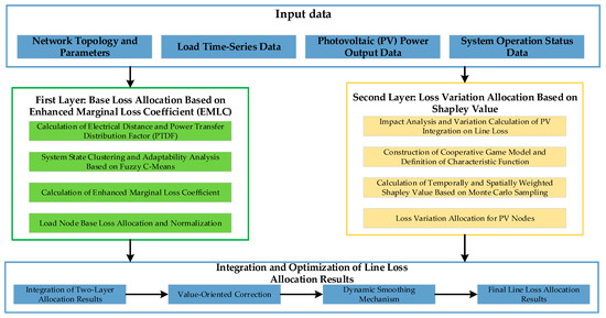
Figure 1.
Framework of the two-stage line loss allocation method for low-voltage distribution networks with distributed photovoltaics.
3.1. Basic Line Loss Allocation Based on EMLC
The physical meaning of the marginal loss coefficient is the amount of change in the total line loss of the distribution network when the power of node i changes by one unit. The basic marginal loss coefficient of node i at time t is defined as
where is the initial power of node i. Through Taylor expansion, the approximate expression for line loss variation can be obtained:
In actual calculations, numerical solutions are usually obtained using the finite difference method:
where ΔP is the introduced small perturbation step size. To improve calculation accuracy, higher-order finite difference methods can also be adopted, such as the central difference method or Richardson extrapolation method. Higher-order formulas have theoretically higher accuracy but also greater computational cost.
In low-voltage distribution networks with distributed photovoltaics, the net injection power of nodes exhibits stronger time-varying characteristics and uncertainty, making marginal loss coefficients significantly different under different operating states. To accurately capture this dynamic characteristic, it is necessary to establish a quantitative characterization method for system states.
This paper defines the distribution network state characteristic vector Φ(t) = [ΦL(t), ΦPV(t), ΦF(t)]T to characterize distribution network operating characteristics from a macro level, where ΦL(t) represents load level characteristics, ΦPV(t) represents PV penetration rate, and ΦF(t) represents reverse power flow proportion (power flow distribution characteristics). Based on historical operating data, distribution network states exhibit obvious clustering characteristics under the dual effects of load changes and PV output fluctuations.
This paper adopts the Fuzzy C-Means Clustering (FCM) algorithm to identify typical operating modes of distribution networks [38,39]. The FCM algorithm solves the optimization problem by alternately optimizing the membership matrix and cluster centers:
where : membership matrix; uih represents the membership degree of sample i to category h; C = {c1, c2, …, cH}: cluster center set, ch is the h-th cluster center; N: number of historical samples; H: number of cluster categories (H = 5 in this paper, representing 5 typical operating modes); m > 1: fuzziness factor, controlling the degree of fuzziness (m = 2 in this paper); ||·||: Euclidean norm.
The membership update formula is
The cluster center update formula is
The algorithm iterates until the change in cluster centers is less than the threshold ε = 10−4.
For the current system state Φ(t) at time t, the membership degree uh(t) to each operating mode category h is calculated through the FCM algorithm. Based on the membership distribution, the state adaptation coefficient is defined as
The physical meaning of αadapt(t) is the degree of closeness between the current operating state and the most similar typical operating mode. The larger the αadapt(t) value, the closer the current state is to an identified typical operating mode.
This paper introduces the node electrical importance coefficient to quantify the influence of nodes in the network. This coefficient comprehensively considers the electrical position of nodes and surrounding load distribution characteristics, defined as
where is the electrical neighboring node set of node i, and is an adaptive threshold, taken as the 75th percentile of electrical distances. This coefficient calculates the influence degree of loads around the node through electrical distance weighting, with neighboring nodes that are closer and have larger load proportions contributing more to the coefficient.
Comprehensively considering system state adaptability and node electrical sensitivity, the Enhanced Marginal Loss Coefficient is defined:
where γe is the weight coefficient of electrical sensitivity, used to balance the influence of system state factors and network topology factors.
Based on the Enhanced Marginal Loss Coefficient, the initial line loss allocation amount of node i ∈ L at time t is calculated as
3.2. Game Theory Incremental Allocation
PV integration changes the power flow distribution and line loss characteristics of distribution networks, further complicating line loss allocation. Traditional methods, such as proportional allocation, are difficult to accurately quantify the true contributions of each node (especially PV nodes) to line loss changes, leading to unfair allocation problems.
The impact of PV nodes on line losses has obvious coalition characteristics, where the combined integration effect of multiple PV nodes is often not equal to the simple superposition of individual node integration effects. For this complex situation of multi-agent interactive influence, cooperative game theory provides a theoretical basis for quantifying the marginal contributions of each PV node and achieving fair incremental line loss allocation. Define the characteristic function v: 2D → R representing the value of PV coalition S ⊆ D:
where is the baseline line loss of the distribution network without any PV integration, and Eloss(S) is the distribution network line loss when only PVs in coalition S are integrated, and all other PVs are not integrated.
In cooperative game theory, the marginal contribution of participant i to coalition S is defined as v(S ∪ {i}) − v(S), representing the incremental value (in this paper, the line loss reduction amount) brought by adding node i to coalition S. This marginal contribution varies depending on which nodes are already present in the coalition, reflecting the complex interactions among PV nodes [40].
The basic requirements of cooperative game theory include the following: (1) Superadditivity: v(S∪ T) ≥ v(S) + v(T), the benefits do not decrease after merging disjoint coalitions; (2) Monotonicity: v(S∪{i}) ≥ v(S), benefits do not decrease as coalition size expands; (3) Individual rationality: ϕi(v) ≥ v({i}), individual gains from joining the coalition are not less than independent action, where ϕi(v) is the benefit of individual i in allocation scheme ϕ.
In the line loss allocation problem with distributed photovoltaics, although under specific spatiotemporal conditions (such as terminal nodes during 11:00–14:00 periods), instantaneous local line loss increases due to reverse power flow may violate the monotonicity assumption, i.e., situations where v(S ∪ {i}) < v(S) exist, analysis based on 24 h cumulative effects shows that situations violating monotonicity account for a low proportion, mainly concentrated in terminal large-capacity PV nodes during high output periods of 11:00–14:00. Most periods and nodes still satisfy the loss reduction effect, and the net contributions of all PV nodes are loss reduction, with instantaneous loss increases being offset by loss reduction effects in other periods. Overall, the basic requirements of cooperative games are still satisfied, so the standard Shapley value method can be directly adopted.
The Shapley value method is a value allocation approach with solid theoretical foundation in cooperative games, satisfying the following fairness principles: (1) Efficiency: The sum of all participants’ Shapley values equals the total coalition benefit, i.e., , ensuring complete cost recovery without surplus or deficit; (2) Symmetry: If two participants have identical marginal contributions to all coalitions, their Shapley values are also identical; (3) Null player property: A participant whose marginal contribution to all coalitions is zero will also have a Shapley value of zero, ensuring that only actual contributors bear responsibility; (4) Additivity: For two games that can be merged, the Shapley value in the merged game equals the sum of Shapley values in the individual games, supporting consistency across different evaluation criteria [41].
The Shapley value method allocates total benefits by calculating the weighted average of each participant’s marginal contributions when joining all possible coalitions:
The weight in the Shapley value formula represents the probability that coalition S is formed before node i joins, when considering all possible node access sequences. Coalitions of the same size receive equal consideration weight, preventing bias toward early or late joiners. This ensures that each PV node’s allocation reflects its average contribution across all possible access scenarios, rather than depending on an arbitrary access sequence.
In the line loss allocation problem, Shapley values quantify each PV node’s fair share of line loss variation by averaging its loss reduction contribution across all possible combinations of PV nodes. For example, the loss reduction contribution of PV node i when it exists alone differs from its contribution when nodes {j, k} are already operating; the Shapley value considers both these scenarios and all other scenarios, deriving a comprehensive allocation result based on fairness through weighted averaging [42].
When the number of PV nodes is large, the complexity of precisely calculating Shapley values is O(|D|·2|D|), making the computational cost expensive. This paper adopts the Monte Carlo sampling method to approximately calculate Shapley values [43]:
where M is the number of samples, and is the coalition excluding i randomly selected in the m-th iteration, reducing the total calculation times from exponential level 2|D| to linear level M * |D|.
Considering the spatiotemporal characteristics of nodes, spatiotemporal weighted Shapley values are introduced:
where yspatial ∈ [0, 0.2] is the adjustment coefficient for spatial correlation, controlling the intensity of spatiotemporal correction. is the local correlation between node i and its surrounding loads, which can be defined as
where is the temporal correlation coefficient between PV output of node i and load of node j, and is the weight based on electrical distance.
Since spatiotemporal weighting modifies the original Shapley value proportions, renormalization is required to maintain efficiency:
3.3. Comprehensive Model of Hierarchical Line Loss Allocation
- (1)
- Baseline Establishment
The first stage establishes the baseline line loss distribution by performing power flow calculations with all PV outputs set to zero () while maintaining actual load levels . This baseline reflects the inherent line loss characteristics of the distribution network determined solely by topology, impedance parameters, and load patterns.
For each load node i ∈ L, the first stage calculates the allocation amount based on the Enhanced Marginal Loss Coefficient: .This calculation is independent of PV characteristics and satisfies the constraint: .
- (2)
- Baseline-Referenced Incremental Allocation
The second stage quantifies the deviation in line loss caused by PV integration relative to the first-stage baseline. The key interaction point lies in the explicit reference to baseline loss in the characteristic function definition: , where is the baseline loss from the first layer, and Eloss(S) is the distribution network line loss when only PVs in coalition S are integrated while all other PVs remain disconnected. This characteristic function measures the loss reduction value contributed by coalition S relative to the first-stage baseline.
The total line loss variation at time t is: , thereby establishing an explicit mathematical dependency: the second stage cannot operate without the first-stage baseline.
This variation is allocated through spatiotemporal weighted Shapley values: , satisfying the efficiency property of the Shapley value method: .
- (3)
- Final Allocation
Combining basic line loss allocation and line loss variation allocation, a hierarchical comprehensive allocation model is constructed. For different types of nodes, their final line loss allocation amounts are calculated as follows:
For pure load nodes (without PV): maintaining the first-stage allocation unchanged,
For pure PV nodes (without load): receiving only the second-stage allocation (typically negative values, representing loss reduction contributions),
For hybrid nodes (with both load and PV): hybrid nodes receive superposition of both stages,
The cost recovery constraint is maintained throughout the entire process: .
The sequential dependency between layers reflects fundamental causality: PV integration causes line loss variations relative to the baseline state. By separating baseline allocation (representing original network responsibility) from incremental allocation (representing PV-induced changes), this method achieves: (1) Clear responsibility separation, preventing cross-subsidization between load users and PV owners; (2) Fairness across entity types through differentiated but complementary evaluation criteria; (3) Physical interpretability, where each allocation component has clear meaning associated with specific operating scenarios.
Dynamic changes in power system operating environments may cause dramatic fluctuations in line loss allocation results, affecting user acceptance. This paper introduces an exponential smoothing mechanism:
where λS ∈ (0, 1] is the smoothing coefficient, controlling the trade-off between current allocation results and historical allocation results. Smaller λS values produce smoother allocation sequences, while larger λS values make allocation results reflect system changes more promptly.
3.4. Multi-Dimensional Value-Oriented Line Loss Allocation Correction Mechanism
3.4.1. Architecture of Multi-Dimensional Value Correction System
Although hierarchical line loss allocation can accurately quantify the actual contributions of each node to line losses, allocation mechanisms based solely on physical causal relationships find it difficult to reflect the diversified value attributes of distributed photovoltaics. The multi-dimensional value-oriented correction mechanism constructed in this section aims to organically combine fair allocation with efficiency optimization. By quantifying the value contributions of PV nodes in three dimensions—local consumption, spatiotemporal matching, and voltage support—and transforming them into differentiated adjustments in line loss allocation, clear economic incentive signals are formed. This incentive mechanism can guide distributed photovoltaics to optimize toward more efficient directions in siting, capacity configuration, and operation strategies without compromising the fairness of physical allocation, thereby improving the overall operational efficiency of the distribution system in the long term.
Specifically, this mechanism achieves efficiency improvement through the following pathways: (1) Local consumption value incentives guide PV configuration closer to load centers, reducing long-distance transmission losses; (2) Spatiotemporal matching value incentives promote coordination between PV output and load demand in temporal and spatial dimensions, reducing long-distance, high-power transmission losses during peak periods; (3) Voltage support value incentives encourage PV to improve system voltage quality through reactive power regulation, reducing additional losses caused by voltage deviations and long-distance reactive power transmission. Through the adaptive Softmax weighting algorithm, this mechanism can dynamically adjust the incentive intensity of different value dimensions according to real-time system operating conditions, ensuring that economic signals always point toward the direction that the system most needs to improve.
Based on this, define the value correction coefficient μi(t) to adjust physical allocation:
where is the physical allocation result obtained in Section 3.3. The correction coefficient is designed using the mean deviation method:
where Xi is the value indicator of node i, is the average value of all PV nodes, and ak ∈ [0, 0.1] controls the correction intensity. When node values are above average, positive incentives are given; when below average, negative incentives are given, achieving a bidirectional incentive mechanism. The design principles of the correction coefficient include:
- (1)
- Maintaining unchanged total line loss allocation of the distribution network to ensure cost recovery.
- (2)
- Forming clear economic incentive signals to guide system optimization, but only fine-tuning the basic allocation rather than making fundamental changes.
3.4.2. Multi-Dimensional Value Assessment
- Local Consumption Service Value Assessment
The local consumption capability of distributed photovoltaics is directly related to the reduction in transmission losses, reflecting significant economic value. This paper evaluates this economic contribution by quantifying the local consumption effect of PV generation.
The instantaneous local consumption rate of node i is defined as
where ϵ is a small positive number to avoid division by zero. This indicator reflects the proportion of PV generation directly consumed by local loads; the higher the consumption rate, the better the effect of reducing long-distance transmission. Further considering the network location characteristics of nodes, introduce the distance attenuation factor:
This factor reflects the density of loads around the node; the denser the loads and the closer the distance, the greater the local consumption potential. Considering the temporal dimension of consumption effects, define the weighted local consumption indicator:
This indicator better reflects actual consumption contributions through PV generation weighting. Based on local consumption contributions, design the local consumption correction coefficient for node i:
where aLCR ∈ [0, 0.1) is the local consumption value conversion coefficient, and is the average of weighted local consumption indicators for all PV nodes.
- 2.
- Spatiotemporal Matching Optimization Value Assessment
The spatiotemporal matching degree between photovoltaics and loads directly affects system resource utilization efficiency and is a key factor in measuring environmental benefits. Good spatiotemporal matching can reduce energy waste and improve overall system environmental performance. This paper proposes a multi-dimensional spatiotemporal matching index that comprehensively considers temporal correlation, power balance, and electrical distance:
where is the weighted comprehensive temporal correlation between PV output of node i and all loads within its electrical neighborhood, is the power imbalance degree, and reflects the electrical centrality of node i in the network.
, and are node-specific weight coefficients satisfying , which can be adaptively adjusted based on entropy weight method algorithms [44].
Based on spatiotemporal matching degree, calculate the spatiotemporal matching correction coefficient for node i:
where aTSM ∈ [0, 0.1) is the time-varying conversion coefficient for spatiotemporal matching value, and is the average of spatiotemporal matching indices for all PV nodes.
- 3.
- Voltage Support Capability Value Assessment
Distributed photovoltaics provide voltage support services to the grid through reactive power regulation and active power control capabilities, reflecting important technical value. This paper systematically quantifies the voltage support contributions of PV nodes to evaluate this technical dimension value.
The voltage support capability of PV nodes needs comprehensive evaluation under multiple operating scenarios:
where Q is the set of different reactive regulation levels, πq is the weight of regulation level q satisfying , and is the system voltage quality improvement of node i under regulation level q relative to the baseline state.
Considering the topological importance of nodes in the network, introduce the position enhancement factor:
where BCi is the betweenness centrality of node i, measuring the transit importance of the node in the network; ζ ∈ [0, 0.3] is the adjustment coefficient.
Further considering the time-varying characteristics of system voltage support demand, introduce voltage support demand weight:
where σvolt(t) is the standard deviation of system voltage deviations at time t, is the average voltage deviation level, and βvolt ∈ [0, 0.4] is the time-varying adjustment coefficient. This weight reflects that voltage support services have higher technical value during periods when system voltage quality is poor.
Comprehensively considering basic support capability, topological importance, and time-varying demand, define the weighted voltage support indicator:
This indicator better reflects actual technical support contributions through PV generation weighting.
Based on voltage support contributions, calculate the voltage support correction coefficient for node i:
where αVS ∈ [0, 0.1) is the voltage support value conversion coefficient, and is the average of weighted voltage support indicators for all PV nodes.
3.4.3. Line Loss Allocation Mechanism with Multi-Dimensional Value Synergistic Correction
Based on the special requirements of multi-dimensional value correction in distribution network line loss allocation, this paper proposes a node-level adaptive Softmax weighting algorithm. Compared with linear normalization methods [45], Softmax naturally guarantees weight non-negativity through exponential functions; compared with the Analytic Hierarchy Process (AHP) [46], it avoids tedious pairwise comparison processes, reducing computational complexity from O(K3) to O(K); compared with the entropy weight method [47], the temperature parameter τ of Softmax provides a more flexible weight distribution control mechanism [48]. In particular, the introduction of the temperature parameter enables the algorithm to dynamically adjust weight concentration according to different node characteristics, which is especially important in the complex scenarios of distribution network line loss allocation. The algorithm dynamically allocates weights for value dimensions based on the characteristics of different nodes:
where is the importance indicator vector of node i at time t, represents local consumption importance, represents spatiotemporal matching importance, where CVloss(t) is the coefficient of variation in line loss distribution, and represents voltage support importance.
The Softmax function converts importance indicators into normalized weights:
where τ is the temperature parameter controlling the smoothness of weight distribution. Smaller τ values make weight distribution sharper, highlighting dominant dimensions; larger τ values make weight distribution more uniform. This paper adopts τ = 1.0 to achieve a balance between highlighting dominant dimensions and maintaining equilibrium. To ensure algorithm robustness, input importance indicators are normalized as preprocessing (scaled to the [0, 1] interval), and through the limitation of value correction intensity coefficient ak ∈ [0, 0.1], it is ensured that value-oriented corrections adjust physical allocation results within ±5%.
Combining the three dimensions of local consumption, spatiotemporal matching, and voltage support, calculate the comprehensive correction coefficient for node i:
To ensure unchanged total line loss allocation of the distribution network, perform normalization:
The final result of value-oriented line loss allocation for PV nodes is
Line loss allocation for non-PV nodes remains unchanged:
The value-oriented line loss allocation correction mechanism transforms the multi-dimensional values of distributed photovoltaics into economic incentive signals, providing an effective pathway for coordinated optimization between distributed photovoltaics and the grid.
4. Simulation Verification and Analysis
4.1. Test System Construction
The simulation analysis in this paper uses the standard low-voltage test network developed by CIGRE (Conseil International des Grands Réseaux Électriques/International Council on Large Electric Systems) Task Force C6.04.02 [49]. During the modeling process, this paper referenced the low-voltage distribution network modeling methodology based on cluster analysis of actual grids from reference [50]. The CIGRE low-voltage network used is implemented through the open-source power system analysis tool pandapower [51]. This network includes 44 bus nodes, 37 distribution lines, 3 distribution transformers, 15 load connection points, and 3 switching devices, with complete network topology and geographical coordinate information, capable of fully reflecting the structural characteristics and operational properties of typical low-voltage distribution networks.
As shown in Figure 2, the CIGRE low-voltage test network consists of one main node (node 0) and three sub-networks: residential area (R nodes), industrial area (I nodes), and commercial area (C nodes). The network includes 44 nodes and 45 lines. The improved network maintains the basic structure of the CIGRE standard test network while optimizing load distribution, adding distributed PV integration points, and configuring differentiated typical daily load curves for industrial, commercial, and residential areas. The total installed PV capacity is 260 kW, accounting for approximately 38% of the total system load, conforming to a medium PV penetration scenario. The selection of PV nodes considers different network positions (main line/branch/terminal) and different capacity ratios to comprehensively evaluate the performance of the method. Figure 3 shows the PV output curve and load curves for different areas. Residential loads exhibit typical “morning and evening double peak” characteristics, with morning peaks occurring at 7:00–9:00 and evening peaks at 19:00–21:00; industrial loads remain relatively stable during working hours (8:00–17:00); commercial loads reach peaks during business hours (8:00–18:00). This study adopts Monte Carlo simulation methods, introducing random multiplier factors following normal distribution N(1, 0.1) in the PV output model to characterize random fluctuations caused by natural factors such as cloud shading. The orange area in Figure 3 represents the possible range of PV output after considering random factors. The temporal relationships between regional loads and PV output directly affect line loss distribution characteristics.
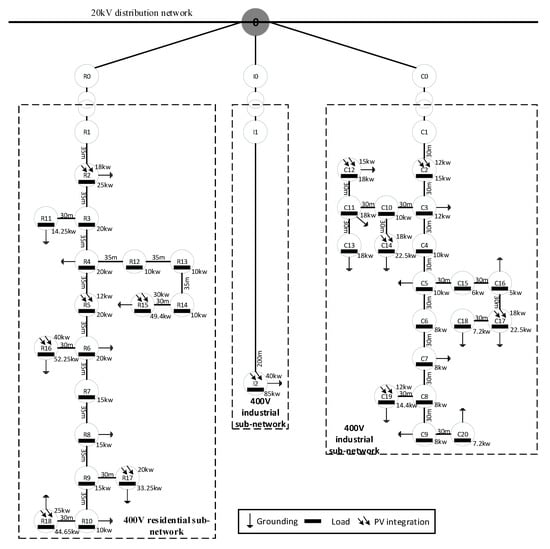
Figure 2.
Improved CIGRE low-voltage test network topology.
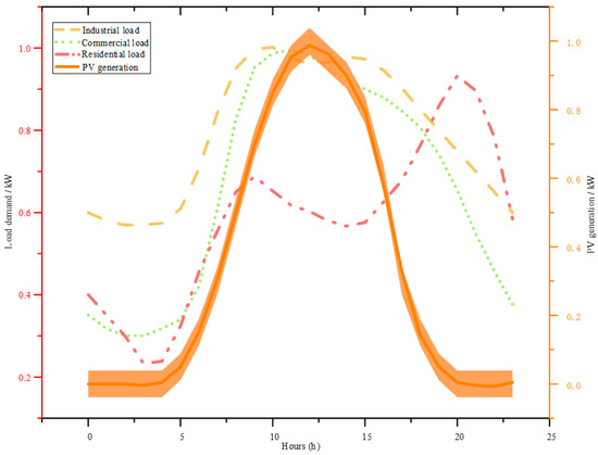
Figure 3.
Comparison of load temporal characteristics curve with photovoltaic generation.
4.2. Impact Assessment of PV Integration on Line Losses
Figure 4 compares the 24 h line loss variation curves under two scenarios, with and without PV.
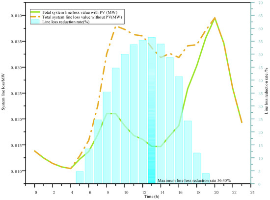
Figure 4.
Dynamic changes in distribution network line losses with and without photovoltaics.
In the scenario without PV, the line loss curve basically follows the trend of load curve changes, with line loss peaks occurring during load peak periods. After PV integration, line losses during daytime periods (8:00–16:00) are significantly reduced, with a maximum reduction of 56.5%; while during nighttime periods, line losses remain basically unchanged due to no PV generation. Overall, PV integration reduces the total daily line loss of the distribution network from the original 0.645 MWh to 0.472 MWh, a reduction of 30.8%.
Further analysis reveals that the line loss reduction effect is closely related to the degree of spatiotemporal matching between PV and loads. The commercial area, due to its load peak being relatively consistent with the PV output peak, shows the most significant line loss reduction effect, with a unit capacity (per MW) PV loss reduction effect of 106.67%; while the residential area’s evening peak load cannot be directly supported by PV, resulting in a weaker line loss reduction effect with a loss reduction effect of 53.61%.
It is worth noting that during certain periods (such as 11:00–14:00), reverse power flows occurred in some areas (mainly terminal nodes in residential areas), leading to slight increases in local line losses, verifying the spatiotemporal characteristics of PV impact on line losses.
4.3. Node Shapley Value Analysis
Figure 5 compares the original Shapley values with the results after spatiotemporal weighted correction.
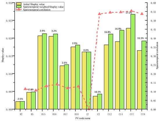
Figure 5.
Comparison of Temporal–Spatial Weighted Correction Effects on Shapley Values.
The simulation results verify the conclusions of the cooperative game applicability analysis in Section 3.2, where all PV nodes have positive Shapley values, indicating that each node’s net contribution to the overall system line loss during the 24 h operation cycle is a loss reduction. Commercial area nodes (C prefix) generally receive higher positive corrections (average +16.8%), while residential area (R prefix) nodes have smaller correction magnitudes (average +2.7%), which is consistent with the differences in matching degrees between load curves and PV output in different areas. Spatiotemporal weighted correction does not change the sign of Shapley values; all nodes maintain positive values before and after correction, with only moderate adjustments in magnitude based on spatiotemporal correlations. Nodes with high spatiotemporal matching receive greater loss reduction contribution recognition, while nodes with low spatiotemporal matching have relatively reduced loss reduction contributions, but all maintain positive contribution characteristics to system loss reduction. This Shapley value correction method, based on spatiotemporal weighting, organically combines the temporal dimension output characteristics and spatial dimension position attributes of PV nodes, significantly improving the accuracy and specificity of line loss allocation.
4.4. Line Loss Allocation with Multi-Dimensional Value Synergistic Correction
This study conducted quantitative evaluations of local consumption rate, spatiotemporal matching degree, and voltage support capability for PV nodes, with results shown in Figure 6.
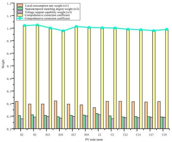
Figure 6.
Comparison of multi-dimensional value weights for PV nodes.
All nodes have generally high local consumption rate contribution weights (0.36–0.42), while spatiotemporal matching weights (0.29–0.32) and voltage support capability weights (0.27–0.32) are relatively lower. This indicates that local consumption rate benefits dominate in the overall value assessment. Value correction proportions are controlled within ±5%, sufficiently moderate, with some nodes receiving positive corrections while others receive negative corrections. This demonstrates that value-oriented correction makes fine adjustments to the allocation without replacing the basic method of hierarchical line loss allocation, and can show clear distinctions based on nodes’ value contributions.
Combining hierarchical physical allocation and multi-dimensional value correction, the final line loss allocation results are obtained, as shown in Figure 7, detailed hierarchical loss allocation data for each node are provided in Appendix A Table A1. Experimental results show that the first layer allocation based on Enhanced Marginal Loss Coefficient (EMLC) presents significant spatial dependency characteristics, with remote nodes (R15, R16, C17) having significantly higher allocation amounts than near-end nodes (R2, C2), which is highly positively correlated with node enhanced MLC values, verifying the accurate capture capability of the proposed method for network topology sensitivity.
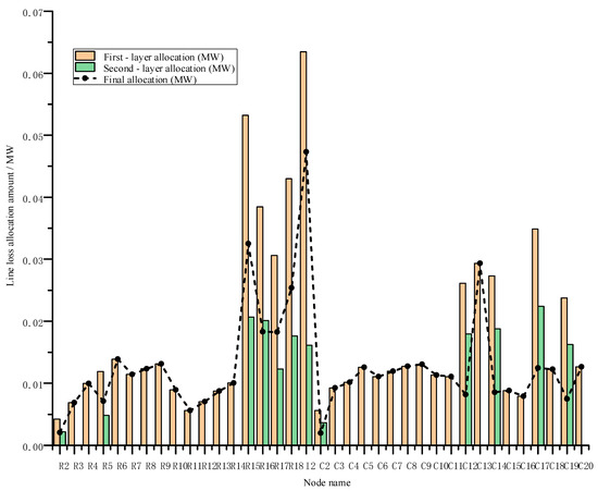
Figure 7.
Comparison of results from the two-stage line loss allocation model.
The second layer allocation results based on spatiotemporal weighted Shapley values effectively quantify the contributions of PV nodes to line loss changes. Experimental data show that most PV nodes receive positive incentive compensation, with C17, C14, and C12 nodes receiving the highest compensation values, which directly correspond to their high spatiotemporal weighted Shapley values. This phenomenon quantitatively confirms the key role of spatial position in line loss contribution assessment.
Pure load nodes (R3, C3, etc.) maintain final allocation amounts consistent with first-layer allocation; while PV hybrid nodes achieve significant allocation reductions, with I2 node reduction reaching 25.46%, R15 node reduction of 38.88%, and C17 node reduction reaching 64.2%. This graded differentiated allocation pattern reflects the precision of the method.
4.5. Horizontal Comparative Analysis with Existing Methods
Figure 8 shows the differences in node allocation between the proposed hierarchical allocation method and the power flow tracing method, marginal loss coefficient method, and graph theory–power flow method [21,26,28]. Table 1 presents the different line loss allocation values for several major PV nodes in the system under different allocation methods.
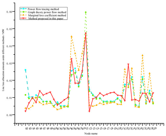
Figure 8.
Comparison of line loss allocation using different methods.

Table 1.
Comparison of line loss allocation values for major PV nodes under different methods.
For commercial area nodes (C2, C12, C17, C19, etc.) with high temporal matching between PV output and load demand, the proposed method reasonably reflects their contributions to line loss reduction through spatiotemporal weighted Shapley values and multi-dimensional value correction mechanisms. For example, the allocation amount for node C12 is 0.008185 MW, representing a 53.3% improvement over the power flow tracing method, 69% improvement over the graph theory–power flow method, and 50% improvement over the marginal loss coefficient method. Traditional methods based on network topology and load states lead to excessively high allocation values for terminal high-load PV nodes (R16, C17, C19, etc.). The proposed method effectively separates PV contributions through hierarchical allocation, reducing line loss allocation for remote high-load PV nodes. For example, the allocation amount for node R16 is 0.01831 MW, representing a 32% improvement over the power flow tracing method, 48.5% improvement over the graph theory–power flow method, and 24.5% improvement over the marginal loss coefficient method, effectively avoiding unreasonable penalties on remote distributed PV nodes. It is worth noting that residential area terminal nodes (such as R17, R18) have higher allocation values under the proposed method compared to power flow tracing and graph theory–power flow methods, but this is reasonable: R17 and R18 have large loads but poor PV-load spatiotemporal matching in residential areas (no PV support during residential evening peak periods), and power flow tracing methods underestimate the actual contributions of PV nodes. The total allocation error for all methods is less than 0.1%, satisfying the cost recovery principle.
Compared with the power flow tracing method, MLC method, and graph theory-based power flow tracing method, the hierarchical structure adopted by the proposed method clearly separates baseline line losses without PV from line loss variations after PV integration. The allocation to pure load nodes reasonably reflects their electricity demand, and the allocation to PV nodes accurately quantifies their marginal contributions to line loss variations, making the allocation process possess clearer physical meaning. This differentiated allocation guides optimal configuration of distributed photovoltaics in locations with good spatiotemporal matching.
4.6. Robustness Comparative Analysis
This study adjusted PV penetration rate from the baseline scenario (38%) to low penetration (20%) and high penetration (60%) levels, respectively, observing the variation trends and sensitivity characteristics of final line loss allocation amounts for various node types.
Figure 9 shows the final line loss allocation amounts for each node under three PV penetration rate levels. Results indicate that as PV penetration rate increases, overall system line losses show a downward trend, but different types of nodes exhibit different behaviors. Node line loss allocation presents a dual response pattern, with terminal PV nodes (C12, C14, C17, C19, R15–R18, I2) showing significant allocation reductions under high penetration rates, while front-end load nodes (C3–C9, R6–R14) have line loss allocations that increase slightly with penetration rate increases, indicating that under high penetration conditions, increased reverse power flows lead to line loss increases.
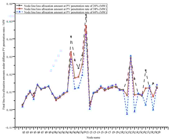
Figure 9.
Comparison of final line loss allocation for nodes at different penetration levels.
Table 2 and Table 3, respectively, show robustness indicator comparisons with and without PV nodes, including average node coefficient of variation (CV) [52,53], median node CV, average node QCD (Quartile Coefficient of Dispersion), average maximum deviation %, and average variation range.
Table 2.
Robustness indicators for all nodes.
Table 3.
Robustness indicators for load nodes.
As shown in Table 2, the average CV value (0.1664) of the proposed method is slightly higher than comparative methods when including PV nodes, but the median CV is only 0.0402, significantly lower than other methods. This indicates that the proposed method maintains excellent robustness for most nodes, while the higher average CV is due to high CV values for PV nodes. However, this precisely embodies the principle of “who caused the incremental part of loss, who is responsible for it” that PV nodes should follow in our method. The allocation amounts for PV nodes sensitively respond to penetration rate changes (as shown in Figure 7, C2 is 0.003609 MW at 20% penetration rate, 0.001997 MW at 38% penetration rate, and drops to 0.000239 MW at 60% penetration rate), accurately reflecting the dynamic impact of PV output fluctuations on line losses. In contrast, other methods “smooth” this fluctuation across all nodes, which, although appearing statistically stable, actually obscures the true physical causal relationships.
Table 3 shows that after removing PV nodes, the average CV of the proposed method drops to 0.0325, significantly better than other methods, proving that the stability of the proposed method in pure load scenarios is comparable to or even superior to traditional methods.
The robustness characteristics of the proposed method can be summarized as “differentiated stability”–exhibiting excellent stability for pure load nodes while accurately identifying dynamic characteristics for PV nodes. This characteristic makes the proposed method more physically meaningful and practically valuable in high-proportion distributed photovoltaic integration scenarios.
5. Conclusions
This study conducted comprehensive verification of the hierarchical line loss allocation model for low-voltage distribution networks with distributed photovoltaics based on the improved CIGRE low-voltage test network. Research results show that distributed PV integration has a significant impact on low-voltage distribution network line losses. Good PV-load spatiotemporal matching can substantially reduce distribution network line losses, while poor matching may cause reverse power flows to increase local line losses. The proposed Enhanced Marginal Loss Coefficient effectively captures system time-varying characteristics and node topological characteristics. Compared with traditional MLC, it considers the dual dimensions of system state adaptability and electrical sensitivity, providing a more precise theoretical basis for basic line loss allocation. Meanwhile, the spatiotemporal weighted Shapley value method achieves fair allocation of PV line loss variations by integrating the spatiotemporal characteristics of PV nodes into the allocation process.
The multi-dimensional value correction and adaptive Softmax weighting mechanisms constructed in the study successfully transform PV local consumption rate, spatiotemporal matching degree, and voltage support capability into economic incentive signals, capable of dynamically adjusting incentive direction and intensity based on node characteristics and system demands. The proposed method transforms fair cost allocation into effective efficiency optimization signals through a three-layer mechanism of ‘precise quantification + multi-dimensional incentives + dynamic response.’ Case studies show that commercial area nodes with high spatiotemporal matching achieve significantly better unit capacity loss reduction effects than residential areas. This efficiency difference is transmitted through differentiated line loss allocation costs, providing continuous momentum for long-term system optimization. Simulation results verify that high-value nodes receive significant allocation reductions. This clear economic signal can guide distributed photovoltaics to optimize toward more efficient directions in siting, capacity configuration, and operation strategies.
The combination of the hierarchical line loss allocation model and value-oriented correction mechanism effectively guides optimal allocation of distributed photovoltaics while ensuring physical rationality and fairness. Case studies validate the effectiveness of the proposed method in line loss allocation problems for low-voltage distribution networks with distributed photovoltaics, providing theoretical support and methodological guidance for constructing more fair, efficient, and sustainable distribution network operation mechanisms.
It should be noted that no single line loss allocation method is universally optimal; different methods exhibit distinct advantages depending on application contexts. The proposed method performs well for distributed photovoltaic integration in low-voltage networks, particularly with high PV penetration (>20%), strong load variability, and refined incentive requirements. However, computational complexity is higher than traditional methods due to Shapley value calculations, making traditional methods preferable for low penetration (<10%) or stable load scenarios. While the framework focuses on photovoltaics, it possesses structural extensibility to other DERs. The first-stage EMLC allocation is technology-agnostic, while the second-stage Shapley framework can accommodate any DER causing quantifiable loss variations. Technology-specific adaptations are required: wind power necessitates modified spatiotemporal metrics and stochastic state characterization; BESS requires redefined characteristic functions and value dimensions, including peak-shaving and time arbitrage; multi-DER systems necessitate hierarchical coalition structures and enhanced computational methods. This research assumes normal operating conditions without explicit reliability constraints. Although system stability is indirectly considered through state adaptability and voltage assessment, integrating reliability constraints with loss allocation remains a future research priority. Future research should explore: (1) joint reliability-loss cost allocation frameworks; (2) dynamic adjustments for aging equipment losses; (3) integration with active control strategies for “allocation-optimization-reliability” collaborative models; (4) systematic validation across diverse DER portfolios; and (5) computationally efficient algorithms using enhanced Shapley estimation methods. These extensions would provide unified theoretical foundations for fair and efficient cost allocation in networks with diverse DER portfolios.
Author Contributions
Conceptualization, Q.P., X.P. and Z.Z.; methodology, Q.P. and X.W.; software, Q.P. and H.Z.; validation, Q.P., X.W. and H.L.; formal analysis, Q.P., H.Z., H.C. and X.W.; investigation, Q.P., X.W. and H.L.; resources, X.P. and Z.Z.; data curation, Q.P., H.Z. and H.C.; writing—original draft preparation, Q.P., H.Z. and X.P.; writing—review and editing, X.P., Z.Z., X.W., H.C. and H.L.; visualization, Q.P. and H.C.; supervision, X.P. and Z.Z.; project administration, X.P. and Z.Z.; funding acquisition, X.P. and Z.Z. All authors have read and agreed to the published version of the manuscript.
Funding
This research was funded by the National Natural Science Foundation of China (Grant No. 62273104) and the Science and Technology Project of Guangdong Power Grid Co., Ltd. (Grant No. GDKJXM20231545).
Data Availability Statement
The original contributions presented in this study are included in the article. Further inquiries can be directed to the corresponding author.
Conflicts of Interest
The authors declare no conflicts of interest.
Appendix A
Table A1.
Hierarchical line loss allocation results for nodes.
Table A1.
Hierarchical line loss allocation results for nodes.
| Node | First Layer Allocation/MW | Second Layer Allocation/MW | Final Allocation/MW | Node | First Layer Allocation/MW | Second Layer Allocation/MW | Final Allocation/MW |
| R2 | 0.00425 | 0.00217 | 0.00208 | C2 | 0.00563 | 0.00364 | 0.00199 |
| R3 | 0.00689 | 0 | 0.00689 | C3 | 0.00928 | 0 | 0.00928 |
| R4 | 0.00998 | 0 | 0.00998 | C4 | 0.01018 | 0 | 0.01018 |
| R5 | 0.01194 | 0.00482 | 0.00711 | C5 | 0.01258 | 0 | 0.01258 |
| R6 | 0.01388 | 0 | 0.01388 | C6 | 0.01107 | 0 | 0.01107 |
| R7 | 0.01145 | 0 | 0.01145 | C7 | 0.01197 | 0 | 0.01197 |
| R8 | 0.01237 | 0 | 0.01237 | C8 | 0.01273 | 0 | 0.01273 |
| R9 | 0.01314 | 0 | 0.01314 | C9 | 0.01307 | 0 | 0.01307 |
| R10 | 0.00893 | 0 | 0.00893 | C10 | 0.01134 | 0 | 0.01134 |
| R11 | 0.00562 | 0 | 0.00562 | C11 | 0.01109 | 0 | 0.01109 |
| R12 | 0.00704 | 0 | 0.00704 | C12 | 0.02613 | 0.01794 | 0.00819 |
| R13 | 0.00874 | 0 | 0.00874 | C13 | 0.02933 | 0 | 0.02933 |
| R14 | 0.01006 | 0 | 0.01006 | C14 | 0.02733 | 0.01877 | 0.00855 |
| R15 | 0.0532 | 0.02068 | 0.03252 | C15 | 0.00882 | 0 | 0.00882 |
| R16 | 0.03844 | 0.02013 | 0.01831 | C16 | 0.00792 | 0 | 0.00792 |
| R17 | 0.0306 | 0.01233 | 0.01827 | C17 | 0.03489 | 0.0224 | 0.01249 |
| R18 | 0.04301 | 0.01763 | 0.02537 | C18 | 0.01229 | 0 | 0.01229 |
| I2 | 0.06348 | 0.01616 | 0.04732 | C19 | 0.02376 | 0.01629 | 0.00747 |
| C20 | 0.01266 | 0 | 0.01266 |
References
- Han, M.Y.; Xiong, J.; Liu, W.D. Spatio-temporal distribution, competitive development and emission reduction of China‘s photovoltaic power generation. J. Nat. Resour. 2022, 37, 1338–1351. [Google Scholar] [CrossRef]
- Shchemeleva, Y.B.; Shchemelev, A.N.; Davidov, S.K. Analysis of the Electrical Energy Losses Structure. In Proceedings of the 2020 International Multi-Conference on Industrial Engineering and Modern Technologies (FarEastCon), Vladivostok, Russia, 6–9 October 2020; pp. 1–5. [Google Scholar]
- Koochaki, M.; Davoudi, M.; Aghtaie, M. A novel loss allocation method applicable for any desired network topology. Electr. Power Syst. Res. 2023, 224, 109733. [Google Scholar] [CrossRef]
- Huang, D.; Zhou, Y.G.; Liu, D.H.; Liang, X.W.; Wu, K.; Li, L. Calculation and analysis of theoretical line loss in low voltage station area based on Adaboost integrated learning. Electr. Meas. Instrum. 2025; in press. [Google Scholar]
- Cheng, L.; Yu, F.; Huang, P.; Liu, G.; Zhang, M.; Sun, R. Game-theoretic evolution in renewable energy systems: Advancing sustainable energy management and decision optimization in decentralized power markets. Renew. Sustain. Energy Rev. 2025, 217, 115776. [Google Scholar] [CrossRef]
- Zhou, Y.; Huang, D.Z.; Li, P.D.; Ji, K.L.; Liu, X.F.; Tan, H. A three-phase power flow model for low-voltage distribution networks considering balanced bus phase asymmetry and photovoltaic access. Electr. Power China 2024, 57, 190–198. [Google Scholar]
- Hou, X.Z.; Wang, S.W.; Su, Y.; Cheng, Y.Y.; Chen, W.L.; Chen, F.Y.; Wu, Z.Y.; Huang, H.C.; He, Y.M.; Yan, W. Daily theoretical line loss rate probability analysis for low voltage distribution networks. J. Chongqing Univ. 2025, 48, 27–37. [Google Scholar]
- Yang, L.; Wang, X.J.; Wang, Z.J.; Zhao, W.H.; Li, P.; Li, M.X. Data-driven Voltage Coordination Control for Low-voltage Distribution Networks with High Household Photovoltaics Penetration. Electr. Drive 2025, 55, 51–60. [Google Scholar]
- Xiao, J.X.; Ye, Y.; Wang, F.; Shen, J.S.; Gao, F. Comprehensive evaluation index system of distribution network for distributed photovoltaic access. Front. Energy Res. 2022, 10, 1–15. [Google Scholar] [CrossRef]
- Tang, W.H.; Huang, K.C.; Qian, T.; Li, W.W.; Xie, X.H. Spatio-temporal prediction of photovoltaic power based on broad learning system and improved backtracking search optimization algorithm. Front. Energy Res. 2024, 12, 1–18. [Google Scholar] [CrossRef]
- Cheng, L.; Peng, P.; Huang, P.; Zhang, M.; Meng, X.; Lu, W. Leveraging evolutionary game theory for cleaner production: Strategic insights for sustainable energy markets, electric vehicles, and carbon trading. J. Clean. Prod. 2025, 512, 145682. [Google Scholar] [CrossRef]
- Wang, L.C.; Yan, R.F.; Saha, T.K. Voltage regulation challenges with unbalanced PV integration in low voltage distribution systems and the corresponding solution. Appl. Energy 2019, 256, 113927. [Google Scholar] [CrossRef]
- Zheng, S. Analysis of Voltage Stability of Receiving-End Power Grid Adapted to Photovoltaic and DC. Master’s Thesis, Nanjing University of Posts and Telecommunications, Nanjing, China, 2021. [Google Scholar]
- Ma, Z.; Chen, H.Y.; Deng, C.; Chen, Y.; Guan, L. Analysis on the Spatiotemporal Distribution Characteristics of the Frequency Response in Large-scale New Energy Access Sending-end Power Grid. Electr. Drive 2025, 55, 56–65. [Google Scholar]
- He, Z.H.; Cao, R.; Liu, H.P.; Zhou, C. Research on improving photovoltaic fault voltage support capability by virtual impedance and reactive current control. Power Capacit. React. Power Compens. 2022, 43, 42–49. [Google Scholar]
- Ren, Y.F.; Zhao, Y.X.; Chen, S.N.; Sun, Q.; Li, M.Y.; Zhang, W.; Liu, L. Compatibility evaluation of photovoltaic and hydroelectric power generation potential in the Beijiang River Basin based on climate resources. Appl. Meteor. Sci. 2025, 36, 164–177. [Google Scholar]
- Chen, H.; Zhang, T.; Pei, H.M.; Shi, W.; Zhang, X.Y. Analysis of distributed photovoltaic power influence on grid voltage and power losses. Electr. Meas. Instrum. 2015, 52, 63–69. [Google Scholar]
- Singh, N.; Mohapatra, A.; Singh, S.N. Loss allocation methods in distribution networks: Present status and challenges. Electr. Power Syst. Res. 2024, 236, 110966. [Google Scholar] [CrossRef]
- Hota, A.P.; Mishra, S.; Mishra, D.P. Active power loss allocation in radial distribution networks with different load models and DGs. Electr. Power Syst. Res. 2022, 205, 107764. [Google Scholar] [CrossRef]
- Atanasovski, M.; Mijoski, T.; Kostov, M.; Arapinoski, B. Real case study of loss allocation in distribution systems with RES. In Proceedings of the 2022 57th International Scientific Conference on Information, Communication and Energy Systems and Technologies (ICEST), Ohrid, North Macedonia, 16–18 June 2022; pp. 1–4. [Google Scholar]
- Wang, Y.H. Research on Allocation of Energy Losses of Distribution System Including Distributed Generation. Master‘s Thesis, North China Electric Power University, Beijing, China, 2013. [Google Scholar]
- Huang, X.; Ouyang, S.; Ma, S.H. Line loss allocation method considering the contribution rate of the distributed generation to distribution network. Electr. Meas. Instrum. 2019, 56, 16–24. [Google Scholar]
- Kumar, H.; Khatod, D.K. Loss allocation in three-phase distribution network using τ-Value. IEEE Trans. Power Syst. 2024, 39, 4924–4934. [Google Scholar] [CrossRef]
- Kumar, H.; Khatod, D.K. τ-Value Based approach for loss allocation in radial and weakly meshed distribution networks with distributed generation. IEEE Trans. Power Deliv. 2022, 37, 1845–1855. [Google Scholar] [CrossRef]
- Gui, J.P.; Zhou, B.T.; Rao, Y.; Wang, W.Z.; Liang, C.; Ding, S.; Xu, C.Y. Loss allocation method for distribution network with DG based on knowledge graph and network topology. J. Wuhan Univ. (Eng. Ed.), 2025; in press. [Google Scholar]
- Liu, W.Y.; Chen, X.X.; Wang, F.Y.; Liu, F.C.; Wang, G. Network loss allocation based on graph theory and power flow tracking. J. North China Electr. Power Univ. (Nat. Sci. Ed.) 2020, 47, 1–9. [Google Scholar]
- Jagtap, K.M. Average marginal loss allocation of distribution networks. In Proceedings of the 2021 13th IEEE PES Asia Pacific Power & Energy Engineering Conference (APPEEC), Thiruvananthapuram, India, 21–23 November 2021; pp. 1–5. [Google Scholar]
- Li, M.Z.; Huo, C.J.; Wang, W.R.; Yu, K.; Zhang, F.R.; Zhang, Y.F. Loss allocation of distribution network with distributed generations based on improved marginal loss coefficients method. Electr. Power Eng. Technol. 2022, 41, 180–184. [Google Scholar]
- Cheng, L.; Wei, X.; Li, M.; Tan, C.; Yin, M.; Shen, T.; Zou, T. Integrating evolutionary game-theoretical methods and deep reinforcement learning for adaptive strategy optimization in user-side electricity markets: A comprehensive review. Mathematics 2024, 12, 3241. [Google Scholar] [CrossRef]
- Zhao, J.; Du, S.; Dong, Y.; Su, J.; Xia, Y. A bidirectional loss allocation method for active distributed network based on virtual contribution theory. Int. J. Electr. Power Energy Syst. 2023, 153, 109112. [Google Scholar] [CrossRef]
- Zare, A.; Mehdinejad, M.; Abedi, M. Designing a decentralized peer-to-peer energy market for an active distribution network considering loss and transaction fee allocation, and fairness. Appl. Energy 2024, 358, 122527. [Google Scholar] [CrossRef]
- Chaitra, A.S.; Sudarshana Reddy, H.R. Improving Reliability in Distribution Systems through Optimal Allocation of Distributed Generators, Network Reconfiguration and Capacitor Placement. SN Comput. Sci. 2024, 5, 456. [Google Scholar] [CrossRef]
- Wilczak, J.M.; Kirk-Davidoff, D.B.; Bloomfield, H.; Bracken, C.; Sharp, J. Wind and solar energy droughts: Potential impacts on energy system dynamics and research needs. J. Renew. Sustain. Energy 2025, 17, 022301. [Google Scholar] [CrossRef]
- Hjalmarsson, J.; Thomas, K.; Boström, C. Service stacking using energy storage systems for grid applications – A review. J. Energy Storage 2023, 60, 106639. [Google Scholar] [CrossRef]
- Mitchell, R.; Cooper, J.; Frank, E.; Holmes, G. Sampling permutations for Shapley value estimation. J. Mach. Learn. Res. 2022, 23, 1–46. [Google Scholar]
- Atanasovski, M.; Taleski, R. Power Summation Method for Loss Allocation in Radial Distribution Networks With DG. IEEE Trans. Power Syst. 2011, 26, 2491–2499. [Google Scholar] [CrossRef]
- Grainger, J.J.; Stevenson, W.D., Jr.; Chang, G.W. Power System Analysis, 2nd ed.; McGraw-Hill Education: New York, NY, USA, 2016; ISBN 978-1-259-00835-1. [Google Scholar]
- Shang, C.; Gao, J.; Liu, H.; Liu, F. Short-Term Load Forecasting Based on PSO-KFCM Daily Load Curve Clustering and CNN-LSTM Model. IEEE Access 2021, 9, 50344–50357. [Google Scholar] [CrossRef]
- Leng, D.; Qiu, Z. Identification of Anomaly Detection in Power System State Estimation Based on Fuzzy C-Means Algorithm. Int. Trans. Electr. Energy Syst. 2023, 7553080. [Google Scholar] [CrossRef]
- Serrano, R. Cooperative games: Core and Shapley value. In Encyclopedia of Complexity and Systems Science; Meyers, R.A., Ed.; Springer: New York, NY, USA, 2009; pp. 1729–1746. [Google Scholar]
- Shapley, L.S. A value for n-person games. In Contributions to the Theory of Games; Kuhn, H.W., Tucker, A.W., Eds.; Princeton University Press: Princeton, NJ, USA, 1953; Volume II, pp. 307–317. [Google Scholar]
- Singh, V.P.; Ahmad, A.; Jagtap, K.M. Weighted Shapley value: A cooperative game theory for loss allocation in distribution systems. Front. Energy Res. 2023, 11, 1129846. [Google Scholar] [CrossRef]
- Touati, S.; Radjef, M.S.; Sais, L. A Bayesian Monte Carlo method for computing the Shapley value: Application to weighted voting and bin packing games. Comput. Oper. Res. 2021, 125, 105094. [Google Scholar] [CrossRef]
- Hu, R.Z.; Lv, S.X.; Zhang, C.; Geng, P.L.; We, H.; Zheng, L.J. Real time comprehensive evaluation method of power quality based on state entropy and dual track TOPSIS. Power Syst. Prot. Control 2023, 51, 102–114. [Google Scholar]
- Patro, S.G.K.; Sahu, K.K. Normalization: A Preprocessing Stage. IARJSET 2015, 20–22. [Google Scholar] [CrossRef]
- Saaty, T.L. Decision making with the analytic hierarchy process. Int. J. Serv. Sci. 2008, 1, 83–98. [Google Scholar] [CrossRef]
- Wang, Y.-M.; Luo, Y. Integration of correlations with standard deviations for determining attribute weights in multiple attribute decision making. Math. Comput. Model. 2010, 51, 1–12. [Google Scholar] [CrossRef]
- Mukhoti, J.; Kirsch, A.; van Amersfoort, J.; Torr, P.H.S.; Gal, Y. Deep Deterministic Uncertainty: A New Simple Baseline. In Proceedings of the IEEE/CVF Conference on Computer Vision and Pattern Recognition (CVPR), Vancouver, BC, Canada, 7 June 2023; pp. 24384–24394. [Google Scholar]
- Barsali, S. Benchmark Systems for Network Integration of Renewable and Distributed Energy Resources; Technical Brochure 575; CIGRE: Paris, France, 2014. [Google Scholar]
- Dickert, J.; Domagk, M.; Schegner, P. Benchmark low voltage distribution networks based on cluster analysis of actual grid properties. In Proceedings of the 2013 IEEE Grenoble Conference, Grenoble, France, 16–20 June 2013; pp. 1–6. [Google Scholar]
- Thurner, L.; Scheidler, A.; Schäfer, F.; Menke, J.-H.; Dollichon, J.; Meier, F.; Meinecke, S.; Braun, M. pandapower—An Open-Source Python Tool for Convenient Modeling, Analysis, and Optimization of Electric Power Systems. IEEE Trans. Power Syst. 2018, 33, 6510–6521. [Google Scholar] [CrossRef]
- Wu, C.; Zhang, X.P.; Sterling, M. Solar Power Generation Intermittency and Aggregation. Sci. Rep. 2022, 12, 1363. [Google Scholar] [CrossRef]
- Wang, L.; Li, Y.; Wang, Y.; Guo, J.; Xia, Q.; Tu, Y.; Nie, P. Compensation Benefits Allocation and Stability Evaluation of Cascade Hydropower Stations Based on Variation Coefficient-Shapley Value Method. J. Hydrol. 2021, 599, 126277. [Google Scholar] [CrossRef]


Disclaimer/Publisher’s Note: The statements, opinions and data contained in all publications are solely those of the individual author(s) and contributor(s) and not of MDPI and/or the editor(s). MDPI and/or the editor(s) disclaim responsibility for any injury to people or property resulting from any ideas, methods, instructions or products referred to in the content. |
© 2025 by the authors. Licensee MDPI, Basel, Switzerland. This article is an open access article distributed under the terms and conditions of the Creative Commons Attribution (CC BY) license (https://creativecommons.org/licenses/by/4.0/).