Abstract
The substantial energy consumption and associated CO2 emissions from industrial operations pose significant environmental and economic challenges for factories and surrounding communities. Within the context of industrial energy management, the steel industry represents a major energy consumer. The imperative to optimize energy use in this sector is driven by a combination of environmental concerns, economic incentives, and technological advancements. This study presents a machine learning model that integrates the whale optimization algorithm (WOA) with multivariate adaptive regression splines (MARS) to forecast electric energy consumption. Utilizing a dataset comprising 35,040 real-world energy consumption records from Gwangyang Steelworks in South Korea, the model was benchmarked against other regression techniques (ridge, lasso, and elastic-net), demonstrating that the proposed WOA-MARS approach achieves a significant improvement in the RMSE (vs. elastic-net or lasso regression techniques) while maintaining interpretability through hinge function analysis. The WOA-tuned MARS model achieves a coefficient of determination (R2) of 0.9972, underscoring its effectiveness for energy optimization in steel manufacturing. The key findings reveal that CO2 emissions and reactive power variables are the strongest predictors.
Keywords:
multivariate adaptive regression splines (MARS); whale optimization algorithm (WOA); ridge (RR), lasso (RL), and elastic-net (ENR) regressions; steelworks electric energy consumption MSC:
62G08; 92B20; 68T20
1. Introduction
As industrialization advances, energy demand correspondingly increases, necessitating the continual adaptation of national policies. Economic growth further intensifies energy consumption, rendering energy both an essential and finite resource. Promoting energy conservation benefits consumers, producers, and overall sustainability, while safeguarding long-term efficiency. The acceleration of economic expansion amplifies the demand for electricity, a fundamental component of daily life and a critical driver of economic development [1]. Environmental challenges stem from the steel industry’s substantial energy consumption and associated CO2 emissions [2]. Carbon dioxide, the principal greenhouse gas, is predominantly released during blast furnace and coking operations, which together account for approximately 70% of total emissions [3,4]. On a global scale, steel production is responsible for nearly 7% of anthropogenic CO2 emissions [5]. To mitigate climate change, advanced technologies are being developed to quantify and reduce energy consumption and CO2 emissions in steel production. Current research focuses on emission-reduction strategies such as carbon capture and the adoption of green hydrogen technologies [6,7,8]. By 2030, these innovative approaches are projected to decrease CO2 emissions by approximately 14–21% and energy consumption by 7–11% [9]. Consequently, forecasting energy demand has become a critical priority for both industrial sectors and national policymakers [10]. Recent research has increasingly employed data-mining techniques to predict energy consumption, utilizing methods such as gradient-boosted machines [11], neural networks [12], time-series models [13], support vector machines [14], regression analysis [15], and deep learning architectures [16]. One study evaluated predictive models, including generalized linear models (GLMs), support vector regression (SVR), k-nearest neighbors (k-NN), random forest, and M5 model trees within a smart city framework [17], although further enhancements in predictive accuracy remain necessary.
In contrast with time-series forecasting methods, which predict future energy demand using lagged variables, this study focuses on estimating instantaneous energy consumption as a function of concurrent operational parameters. The objective is to model the nonlinear relationships between real-time measurements (e.g., reactive power, CO2 emissions, and load type) and energy usage, providing interpretable insights for operational optimization rather than temporal prediction.
This study accurately predicts the electric energy consumption of Gwangyang Steelworks (see Figure 1) using a multivariate adaptive regression splines (MARS) model [18,19,20,21,22,23,24,25], optimized through the whale optimization algorithm (WOA) [26,27,28,29]. To the best of our current knowledge, this specific combination has not yet been explored in the existing literature. For comparative analysis, the same dataset is also evaluated using ridge regression (RR), lasso regression (LR), and elastic-net regression (ENR) techniques [20,21,22,30,31,32,33,34,35]. MARS is a statistical learning approach capable of capturing nonlinearities and variable interactions, evolving from linear models to effectively represent complex relationships [18,19,20,21,22,23,24,25,26,27,28,30,31]. It offers several advantages over both traditional and metaheuristic regression techniques [18,19,20,21,22,23,24,25,30,31,36,37]: (i) straightforward implementation compared with linear regression, (ii) consistent basis functions derived from identical datasets, (iii) ease of interpretability, (iv) ability to handle both continuous and categorical variables, and (v) an explicit mathematical formulation of the dependent variable through fundamental basis functions. This latter characteristic distinguishes MARS from black-box machine learning models such as multilayer perceptrons. Previous studies have demonstrated the effectiveness of MARS in predicting diverse phenomena, including antitumor activity [38], soil organic carbon [39], regolith geochemical grades [40], drilling mud viscosity [41], used car prices [42], benzene concentration [43], and dissolved oxygen levels [44]. However, to date, it has not been applied to predicting the electric energy consumption of Gwangyang Steelworks.
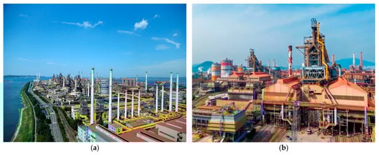
Figure 1.
(a) Aerial view of Gwangyang Steelworks; (b) side view of Gwangyang Steelworks.
The structure of this manuscript is organized as follows: It begins with a detailed description of the experimental design, followed by an outline of the parameters utilized in this investigation. Section 2 provides a comprehensive review of the regression modeling approaches employed, including lasso, ridge, elastic-net, and WOA/MARS-based methods. Section 3 presents the results of the WOA/MARS analysis, comparing predicted values with experimental measurements and evaluating the relative importance of the input parameters. Finally, Section 4 summarizes this study’s conclusions and highlights its principal findings.
2. Materials and Methods
2.1. Experimental Setup
The dataset comprises synchronous measurements of nine independent variables and the target variable (energy consumption (EC)), all recorded at 15 min intervals. The dataset for this study comprises 35,040 samples of electric energy consumption and the following process variables: carbon dioxide emissions (tCO2), lagging current reactive power (LaCRP), lagging current power factor (LaCPF), leading current reactive power (LeCRP), leading current power factor (LeCPF), day of the week (DoW), week status (WS), seconds since midnight (NSM), and load type (LT). The dataset was obtained from the Gwangyang Steelworks, a major industrial facility specializing in the production of steel coils, iron plates, and related steel products [45]. The records span a full year, capturing detailed measurements of key operational variables. The dependent variable in this study is the electric energy consumption (EC), measured in kilowatt-hours (kWh) per 15 min interval. This metric represents the electrical energy used by individual production units or processes within the Gwangyang Steelworks during each sampling period. The 15 min interval aligns with the plant’s data-logging system, capturing high-resolution variations in energy demand associated with operational phases such as smelting, casting, and material handling [46]. The importance of these data comes from their ability to track energy consumption in detail and in real time, providing valuable insights into daily, monthly, and yearly usage patterns [17]. This study does not frame the problem as a time-series forecasting task (e.g., predicting future EC from past values). Instead, the problem is approached as a multivariate regression task, in which EC is estimated from variables measured at the same timestamp. This approach is justified by the industrial need to understand how current operational states (e.g., furnace load and power factor) directly impact energy consumption, without assuming temporal dependencies. Figure 2 shows the experimental setup of the process.
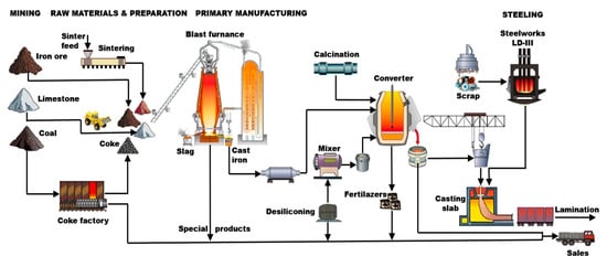
Figure 2.
Schematic diagram illustrating the industrial experimental procedure: experimental setup.
2.2. Variables in Model and Materials
The primary objective of this study was to identify the most influential parameters for estimating energy consumption using the WOA/MARS model. Energy consumption, representing the electrical energy utilized in steel production from iron ore, was designated as the output variable. A total of nine input variables were considered, as summarized in Table 1:

Table 1.
List of the operational variables analyzed in this investigation, gathered with the corresponding standard deviations (STDs) and averages.
Lagging current reactive power (kVarh): Indicates an inductive nature with reactive power consumption when the load current peaks at 90° after the voltage peak;
Leading current reactive power (kVarh): Occurs when the current waveform leads the voltage waveform, indicating capacitive loads supplying reactive power;
Carbon dioxide emission (ton/15 min): Emissions from combustion in steel plants and other industrial processes;
Lagging current power factor (%): Reflects the load current peaking after the voltage, with capacitive loads used to compensate;
Leading current power factor (%): Indicates a capacitive load supplying reactive power when current leads the voltage;
Number of seconds from midnight for each day: Time duration from midnight to the specified datetime value;
Week status: Categorical variable indicating whether the day is a “weekend” or “weekday” [47];
Day of week: Categorical variable indicating the day of the week for casting operations;
Load type: Categorical variable with three types of furnace load: “light load,” “medium load,” and “maximum load”.
The operation output variable of this study was as follows:
The Gwangyang Steelworks’ specific electric energy consumption (kWh): The Gwangyang plant is categorized as a high-energy-consumption facility due to the substantial amount of electrical energy required for steel production.
Exploratory data analysis represents a fundamental step in deriving meaningful insights from a dataset. This analysis confirmed that all dataset features were complete, with no missing values. In addition, the interrelationships among the variables were systematically examined. A correlation matrix was employed to visualize the associations between the different variables, and the corresponding heatmap illustrates the strength of the linear relationships among them. Figure 3 depicts the correlations of various variables with respect to energy consumption. The strongest correlation was observed between CO2 emissions and lagging current reactive power, reflecting their direct relationship with energy consumption.
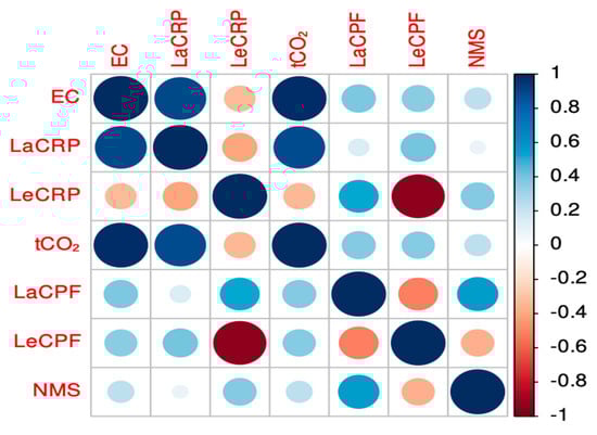
Figure 3.
Correlation matrix for the numerical variables.
2.3. Techniques for Mathematical Modeling
2.3.1. Multivariate Adaptive Regression Splines (MARS) Method
The MARS approach provides a versatile non-parametric approach to regression problems [18,19,20,21,22,23,24,25,30,31]. This technique can be considered as extending both stepwise linear (SL) regression and classification and regression tree (CART) decision trees [30,48,49], while addressing their respective limitations. The primary objective of MARS is to foretell a continuous dependent output variable’s results , relying on a multitude of independent input features, collectively referred to as . The basic principles underlying the MARS methodology can be explained by a specific mathematical formulation [18,19,20,21,22,23,24,25,30,31]:
where
f: This component represents an aggregation of basis functions, each of which depends on the input variable set . These functions are combined by a weighted summation process.
: This term denotes the error vector, which is characterized by its n-dimensional nature, where n corresponds to the number of observations in the dataset. It is typically represented as a column vector with dimensions .
The MARS approach does not necessitate a predetermined functional relationship between the output and input features. Mathematically, it can be articulated as an assemblage of segmented polynomial expressions of order q, referred to as basis functions, with their parameters entirely determined through a detailed analytical process involving .
The methodology of MARS is implemented through the adjustment of specific ranges of the predictor variables using these basis functions. In particular, two-sided truncated power functions, or splines, are the fundamental building blocks of the MARS model. These functions, called hinge functions, can be expressed mathematically as follows [18,19,20,21,22,23,24,25,30,31]:
The hinge function knots in the MARS model are data-derived thresholds optimized to minimize prediction error. These values reflect empirical breakpoints in the relationship between predictors and energy consumption, rather than physical constants.
The power q (where determines how smooth the resulting approximated function is and, at the same time, also determines the category of splines employed. Specifically, when , the model uses linear splines, which are the focus of the present investigation. Quadratic splines are generated when , while cubic splines are generated when , with this pattern continuing for higher values of q. To illustrate this concept, Figure 4 provides a visual representation of two splines in the case where , with the node (also referred to as the knot) positioned at . The purpose of this graphical representation is to demonstrate the behavior of linear splines at a particular node location. The choice of q has significant implications for the flexibility of the model and its capacity to identify nonlinear patterns in the data. Linear splines offer a balance between model simplicity and the ability to approximate nonlinear functions, making them a popular choice in many applications. Higher-order splines can provide greater smoothness but can also introduce additional complexity into the model. The MARS algorithm’s capability to automatically select appropriate basis functions and node locations contributes to its versatility in different areas of scientific investigation.
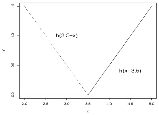
Figure 4.
Graphical representation of linear hinge functions. This figure depicts two linear hinge functions, foundational components of the MARS methodology, commonly referred to as spline foundational components. The diagram includes the following: left spline (dashed line), which represents (x < t, −(x − t)), illustrating behavior for x-values of less than the knot location t; right spline (solid line), which describes (x > t, +(x − t)), characterizing behavior for x-values exceeding t. This visualization highlights the functional symmetry about the knot location t.
Unlike regularized regression methods, the implementation of MARS does not require predictor scaling or centering [50]. The algorithm’s hinge functions adapt to the natural scale of each variable, while the forward/backward selection process ensures parsimony by excluding irrelevant predictors (e.g., unused categorical levels).
The MARS approximation can be characterized as an ensemble of M piecewise linear multivariate splines of a dependent variable derived from M basis functions, built using the hinge functions. The mathematical formulation is as follows [18,19,21,22,23,24,25,30,31]:
where the MARS method’s predicted output variable is and
- represents a constant coefficient, commonly referred to as the intercept;
- signifies the m-th basis function;
- corresponds to the coefficient related to the basis function .
To obtain the optimal collection of basis functions for the comprehensive method, the MARS methodology uses the technique of generalized cross-validation (GCV) [18,19,20,21,22,23,24,25,30,31]. GCV is calculated as the mean-squared residual error divided by a penalty factor, the latter being directly proportional to model complexity, and can be expressed mathematically as [18,19,21,23,24,25,30,31,50,51]
The more basis functions that are employed in the MARS model, the higher the complexity penalizing term, . This term is expressed as [18,19,20,21,22,23,24,25,30,31,50,51]
where M is the number of model basis functions in Equation (3), and d is the model penalty parameter for each basis function.
With the purpose of ensuring the robustness of the findings, it is essential to consider additional factors alongside the aforementioned GCV. These include the following [18,19,21,22,23,24,25,30,31,50,51]:
RSS (residual sum of squares): This measure quantifies the difference between the observations and predictions;
N-subsets: The factor that specifies the total count of groups within the model encompassing all variables.
2.3.2. Ridge Regression and the Least Absolute Shrinkage and Selection Operator (Lasso) Regression Methods
Both regression procedures represent regularization techniques employed in this study to predict the energy consumption (EC) of Gwangyang Steelworks [20,21,22,30,31]. These methods are particularly effective in addressing multicollinearity, which frequently arises in linear regression models with numerous predictors. Overall, they introduce a controlled level of bias in exchange for enhanced efficiency and stability in parameter estimation.
Ridge regression (RR) was developed as a potential solution to address inaccuracies in least squares estimators arising from multicollinearity among independent variables in linear regression models. By providing variance and mean square estimates that are often lower than those obtained via ordinary least squares, RR enables more precise estimation of model parameters. Consequently, it is also employed to predict the energy consumption (EC) of Gwangyang Steelworks [20,21,22,30,31,52,53].
By adding positive components, the problem of a quasi-singular moment matrix is mitigated by lowering the condition number of the diagonals. The following formula for the ordinary least squares estimator can also be used to find the simple ridge estimator [20,21,22,30,31,52,53]:
When is the regressand, represents an identity matrix, with as the design matrix, and the constant that moves the diagonals of the moment matrix is called the ridge parameter , sometimes dubbed as the regularization or complexity parameter. It can be demonstrated that this estimator may be used to solve the following least squares problem with the restriction (a predetermined free parameter t determines the degree of regularization), whereby a Lagrangian can be used to represent it [25,26,27,31,32], as follows:
where . This proves that is just the Lagrange multiplier of the restriction. The ridge estimator turns into ordinary least squares when , demonstrating that the restriction is not enforceable. Typically, is chosen heuristically, which means that it will not exactly meet the requirement. Therefore, the principal advantage of ridge regression over standard linear regression lies in its capacity to balance the trade-off between bias and variance. Specifically, an increase in bias is accompanied by a corresponding reduction in variance, and vice versa.
The lasso regression (LR) method, also applied in this study to address the aforementioned issue, shares several key similarities with ridge regression (RR). The loss function of lasso regression is formally defined as follows [25,26,27,31,32,54,55]:
so that and where the data determines the exact relationship between t and λ.
To sum up, LR can reduce coefficients to zero, whereas RR cannot [20,21,22,30,31,52,53]. This distinction arises from the difference in the shapes of their constraint boundaries. Although they are subject to different constraints— for lasso regression and for ridge regression—both ridge and lasso regression can be interpreted as minimizing a common objective function.
2.3.3. Elastic-Net Regression (ENR)
Elastic-net regression (ENR) combines the principles of both lasso and ridge regressions. The elastic-net Lagrangian function is formulated by integrating the penalty terms of these two methods [20,21,22,30,31,52,53]:
In fact, lasso regression is obtained if , while ridge regression is obtained if . The pair of parameters can be substituted with the parameter, which determines the ratio of the L1 penalty to . Since most computational codes use the number the most, it is used in the calculations here. In this regard, the elastic-net regression’s final Lagrangian is provided by [21,22,31,32,34,35]
2.3.4. Whale Optimization Algorithm (WOA)
The Whale Optimization Algorithm (WOA) was originally proposed by Mirjalili and Lewis [28]. It is an optimization technique inspired by the complex hunting behavior of humpback whales. In a process known as bubble-net feeding, whales generate bubbles to encircle their prey during the hunt. Typically, the whales dive approximately 12 m before creating a spiral of bubbles around the target and subsequently ascend in pursuit. The WOA operates through three primary phases [26,27,28,29]:
Exploration phase: During this phase, each search agent (whale) explores the search space randomly to locate the optimal solution (prey). To update the position of a given search agent, a randomly selected agent is used instead of the current best-performing agent. Mathematically, this behavior is expressed as follows:
where is the position vector of a randomly selected prey, t denotes the actual iteration, and indicates the whale position vector The coefficient vectors are defined as and , with decreasing linearly from 2 to 0 during the iterations, and are random vectors in the range [0, 1]. Exploration is promoted when , forcing whales to move away from a given agent and thereby enhancing the global search ability of the algorithm.
Encircling prey: During the hunting process, humpback whales surround their prey. Other candidate solutions adjust their positions to converge toward the best-performing agent, with the current optimal solution regarded as the global best. Mathematically, this behavior is represented as follows:
where denotes the whale’s position vector, and denotes the position vector of the best solution found so far (the prey). In this case, exploitation is promoted when , ensuring that whales move toward the best solution identified.
Exploitation phase: The objective of this stage is to employ a bubble-net strategy to capture the prey. The bubble-net approach combines two mechanisms: (1) the shrinking encircling mechanism, in which the coefficient vector decreases from 2 to 0 over successive iterations; and (2) the spiral updating position mechanism, which calculates the distance between the whale and the prey and updates the position along a logarithmic spiral:
where is the distance between the whale and the prey, b is a constant defining the shape of the spiral, t is a random number in [−1, 1], and is the prey’s position.
To integrate these two strategies, the WOA assigns a 50% probability of applying either the shrinking encircling mechanism or the spiral updating mechanism in each iteration, which can be formalized as follows:
where p ∈ [0, 1] is a random probability.
In summary, the WOA technique is a very effective tool for solving difficult optimization issues in a variety of fields.
2.4. Goodness of Fit
Nine input variables were employed in the development of the WOA/MARS model, with energy consumption (EC) serving as the dependent variable. The objective was to predict the output variable (SEC) based on these nine process variables and to identify the model that best aligns with the experimental data. The coefficient of determination, R2, was adopted as the primary metric to assess model performance [52,53]. For each data point in the dataset, there exists a corresponding model-estimated value . The observed values correspond to the actual measurements, whereas the predicted values are derived from the model. The variability within the dataset is quantified using the following sums of squares [52,53]:
- First item, total sum of squares (): . This measure is proportional to the sample variance.
- Regression sum of squares (): , sometimes dubbed as the total of squares described;
- Residual sum of squares (): .
In these equations, is the arithmetic mean of the n data points in the experimental dataset and is calculated as
The coefficient of determination is defined as [52,53]
As the statistic approaches unity, it indicates a diminishing disagreement between the experimental and projected data, thus signifying an improved model fit. Similarly, the mathematical expressions for the other two statistics used in this study, root-mean-square error (RMSE) and mean absolute error (MAE), are as follows:
In order to optimize estimation accuracy (R2), this study employs various approximation techniques. These methods model the EC as the dependent variable using nine input factors from experimental samples [47,54]. While the WOA-tuned MARS model was optimized using 10-fold cross-validation to handle its nonlinear structure and hyperparameter tuning, the linear baseline models—ridge regression (RR), linear regression (LR), and elastic-net regression (ENR)—were evaluated on the same independent test set without cross-validation. Given the inherent simplicity of these models and the absence of complex hyperparameters (beyond fixed regularization terms for RR/ENR), a single train–test split (80-20) was deemed sufficient to establish a fair and computationally efficient performance baseline for comparative purposes.
The efficacy of the MARS approximation is heavily contingent upon the selection of its hyperparameters [18,19,21,22,23,24,25,30,31], namely,
- (a)
- Maxfuncs: the highest amount of hinge functions (MF).
- (b)
- The degree to which variables interact (D).
- (c)
- The penalty parameter (d), a GCV parameter imposing a penalty on each node, linked to model complexity (Equation (4)). When d = 0, terms are penalized, but nodes are not; when d = −1, no penalty applies. The common value is d = 2.
- (d)
- The pruned model’s maximum term count (P). The backward pruning stage eliminates ineffective terms to improve model generalization after the forward phase’s overfitting.
To optimize these hyperparameters, this study employs the whale optimization algorithm (WOA) [26,27,28,29]. The WOA is a metaheuristic search algorithm that emulates the hunting behavior of humpback whales in nature, efficiently exploring the hyperparameter search space to identify optimal configurations.
The methodology for implementing the WOA/MARS model is as follows:
Data partitioning: The dataset is bifurcated; twenty percent of the data is employed for testing, while the remaining eighty percent is employed for training.
Model training and hyperparameter optimization:
- (a)
- The training set is utilized to construct the WOA/MARS model.
- (b)
- To adjust the MARS model parameters, a k-fold cross-validation method is used, taking the value k = 10 [52,53,55].
- (c)
- The WOA algorithm is applied within this cross-validation framework to identify the optimal hyperparameter configuration.
Model construction: Once the best parameters are determined, the full training set is employed to construct the final model.
Model evaluation:
- (a)
- The forecasted results are then evaluated against the actual values.
- (b)
- The observed values are then contrasted with these forecasts.
- (c)
- This comparison is used to assess how well the model fits the data.
In this study, several key parameters were defined to implement the WOA and guide the optimization process. The search space parameters are summarized in Table 2. The algorithm was configured with a population size of 40 and a maximum of 50 iterations as the stopping criterion. Unlike certain other optimization methods, this WOA implementation does not use a convergence threshold to terminate the process, relying instead on the predetermined number of iterations.
Table 2.
Search limits of MARS hyperparameters for WOA tuning.
Figure 5 provides a schematic representation of the WOA/MARS-based approximation process utilized in this investigation.
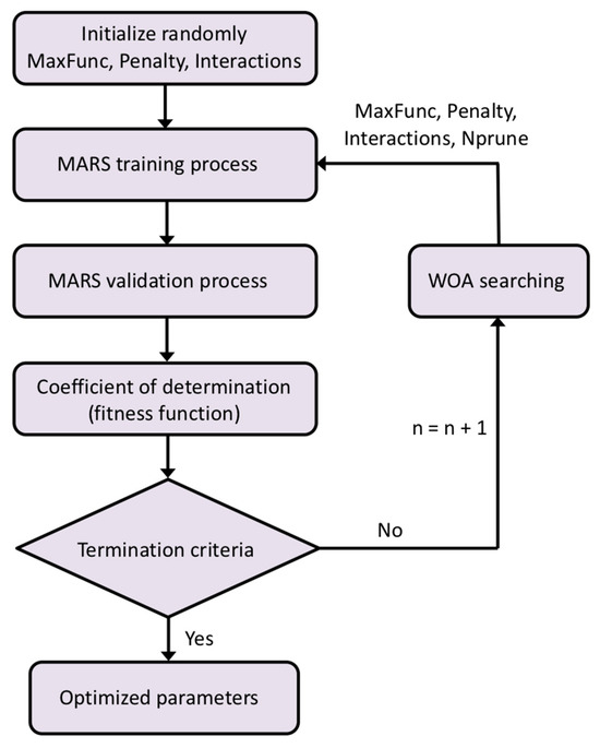
Figure 5.
Flowchart of the WOA/MARS-based approximation.
Predictive modeling frequently uses cross-validation to determine the true coefficient of determination [52,53]. In this investigation, where k = 10, the k-fold cross-validation technique was utilized to assess the predictive capacity of the WOA/MARS-based approximation [52,53,55].
The computational experiments were conducted on an iMac equipped with 24 GB of RAM and an Intel® CoreTM i5-4570 CPU operating at 3.20 GHz with 4 cores. The software environment included the Ubuntu 22.04 operating system, R version 4.5.1, and several key R packages outlined below:
MARS approximation: earth package, version 5.3.4 [56,57];
WOA optimizer: metaheuristicOpt package, version 2.0.0 [28];
RR, LR, and elastic-net regression: glmnet package, version 4.1-9 [58].
The solution space’s variation intervals used in this investigation are displayed below in Table 2.
The WOA metaheuristic optimizer was employed to fine-tune the MARS model parameters, determining optimal values for the upper bound of hinge functions, the level of variable interactions, the penalty parameter, and the maximum number of terms in the pruned model by evaluating cross-validation error differences. The four-dimensional search space corresponds to these four parameters under optimization. The root-mean-square error (RMSE) was adopted as the primary fitness metric and objective function [52,53], providing a robust measure of predictive accuracy for effective parameter evaluation and optimization.
3. Results and Discussion
Table 3 presents the best optimized hyperparameters for predicting electric energy consumption using the MARS-based approach, as found by the WOA optimizer.
Table 3.
Optimized hyperparameters of the most accurately fitted MARS model, as determined by the WOA optimizer, for predicting electric energy consumption (EC).
The primary basis functions and associated coefficients for the optimally adjusted WOA/MARS-based model that was utilized to forecast EC are listed in Table 4. It is important to note that a basis function is defined using the hinge functions that follow the expression [18,19,21,22,23,24,25,30,31,58]:
Table 4.
List of hinge functions and the associated coefficients in the optimally adjusted WOA/MARS-based model for predicting energy consumption.
Fundamentally, MARS represents a type of nonparametric regression technique and can be considered an extension of linear regression. To systematically capture nonlinearities and interactions among input variables, MARS utilizes a weighted sum of the hinge functions described previously [18,19,21,22,23,24,25,30,31].
For comparative analysis, the lasso, ridge, and elastic-net regression techniques were also employed in this study. Their accuracy is contingent upon the parameter [30,32,33,34,35]. Table 5 displays the parameter λ’s ideal value for these regression models, as established by the WOA optimizer.
Table 5.
Optimized λ parameters for lasso, ridge, and elastic-net regression models, as determined by WOA optimization.
To ensure the robustness and validity of the WOA-optimized MARS model, diagnostic analyses of the residuals were performed. Figure 6a presents the residuals versus fitted values plot, which exhibits a random scatter around zero without discernible patterns, confirming the absence of heteroskedasticity and supporting the appropriateness of the model’s functional form. Figure 6b displays the Q–Q plot of the residuals, indicating minor deviations from normality, a phenomenon commonly observed in industrial datasets due to operational outliers. Importantly, these deviations do not impair the model’s predictive performance, as MARS is a nonparametric method that does not rely on the assumption of normally distributed residuals.
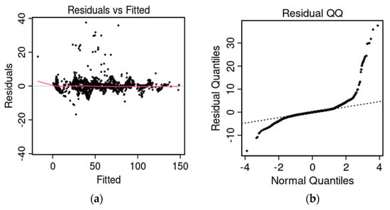
Figure 6.
(a) Residual vs. fitted values graph and (b) Q–Q plot for the WOA/MARS model.
To further assess the interpretability of the model, partial dependence plots (PDPs) were generated for the three most influential variables (CO2, LaCRP, and LaCPF), as presented in Figure 6. These plots depict the relationships between the input variables and the predicted energy consumption, incorporating both first- and second-order terms derived from the WOA-optimized MARS model, thereby elucidating their individual and interactive effects. In Figure 7a, EC (ordinate) is plotted against lagging current reactive power (abscissa), with four other factors kept constant. Similarly, Figure 7b,c show EC versus carbon dioxide emissions and the lagging current power factor, respectively, keeping eight variables fixed. Figure 7d presents a 3D plot of EC (applicate) against carbon dioxide emissions (abscissa) and lagging current reactive power (ordinate), with other variables constant. Likewise, Figure 7e,f depict 3D plots of EC versus carbon dioxide emissions and the lagging current power factor, and lagging versus leading current power factors.
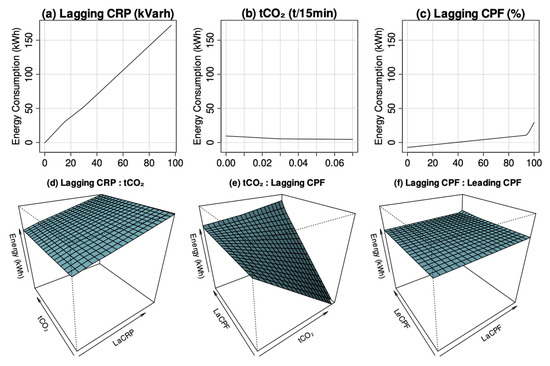
Figure 7.
Visual illustration of the primary and secondary components that constitute the WOA/MARS model for estimating energy consumption: (a) first-order lagging current reactive power term; (b) first-order carbon dioxide term; (c) first-order lagging current power factor term; (d) second-order lagging current reactive power and carbon dioxide terms; (e) second-order carbon dioxide and lagging current power factor terms; and (f) second-order lagging current power factor and leading current power factor terms.
Table 6 summarizes the values of the coefficient of determination (R2), correlation coefficients, and RMSE for various regression models applied to the EC output variable using the testing dataset. The models evaluated include the WOA/MARS-based approach [18,19,21,22,23,24,25,30,31], as well as ridge regression (RR), lasso regression (LR), and elastic-net regression (ENR) [30,32,33,34,35].
Table 6.
Statistical performance indicators (RMSE, MAE, R2, and r) of regression models for EC prediction on the test dataset.
The most recent statistical evaluation indicates that the optimally fitted MARS model achieves an R2 value of 0.9972 and a correlation coefficient (r) of 0.9985 for the EC variable. These results demonstrate a strong agreement between the experimental data and the MARS predictions, indicating a high level of reliability in the model’s goodness of fit. Consequently, this model was selected as the most suitable approach for estimating the dependent variable (EC).
These results are now contextualized by discussing comparable data-driven models reported in the literature. Mubarak et al. [59] introduced a stacked ensemble approach, Stack-XGBoost, which combines multiple machine learning models to predict active and reactive energy consumption in the steel industry. Their methodology employs extra trees regressor (ETR), adaptive boosting (AdaBoost), and random forest regressor (RFR) as base models, with an extreme gradient boosting (XGBoost) algorithm serving as the meta-learner. This approach demonstrated superior accuracy for short-term forecasting horizons. Nevertheless, this MARS model also exhibits strong performance, particularly with respect to the coefficient of determination, indicating an excellent fit to the data. Furthermore, a key advantage of the MARS model is its ability to quantify the importance of each independent variable, providing deeper insights into the factors driving energy consumption predictions.
As a supplementary outcome of these analyses, Table 7 and Figure 7 illustrate the hierarchical importance of the process variables (input factors) in predicting the EC (output dependent factor) [58,60] for this complex investigation.
Table 7.
Ranking of the relevance of the operation variables in the best-fit WOA/MARS model for the EC as stated in the GCV criterion.
In the MARS model, variable importance is estimated using three distinct criteria. First, the nsubsets criterion counts how many model subsets include the variable, with variables appearing in more subsets considered more important. Here, “subsets” refer to the subsets of terms generated during the backward pass of the model-building process. Second, the RSS criterion calculates the decrease in residual sum of squares (RSS) for each subset relative to the previous subset during the backward pass. Variables causing larger net decreases in the RSS are deemed more important. Third, the GCV criterion operates similarly to RSS but uses generalized cross-validation (GCV) instead of the RSS. This criterion was employed to determine variable importance. Both the GCV and RSS columns are normalized so that the largest net decrease is set to 100, facilitating comparison.
Within the MARS framework, carbon dioxide emissions (tCO2) were identified as the most influential predictor of the output variable EC. This is followed, in descending order of importance, by the lagging current reactive power (LaCRP), the lagging current power factor (LaCPF), and the leading current power factor (LeCPF). It is noteworthy that the remaining input variables were not included in the model as explanatory factors.
Figure 8 illustrates the proportional significance of process variables in the optimally fitted WOA/MARS-based approach for EC prediction, determined by the generalized cross-validation (GCV) criterion.
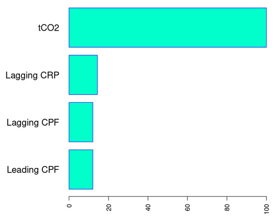
Figure 8.
Variable importance in the optimal WOA/MARS model for EC prediction according to GCV criterion.
In steel plants, electrical energy consumption plays a critical role in production efficiency. Among the influencing factors, CO2 emissions are the most significant, as they exhibit a direct correlation with energy usage, particularly in high-temperature operations and fossil fuel combustion processes [61]. The generation of CO2 serves as an indicator of both energy consumption and process efficiency.
Lagging current reactive power, the lagging current power factor, and the leading current power factor exert a secondary influence, primarily affecting power quality and equipment efficiency rather than total energy consumption. While reactive power impacts supply stability, its effect is less pronounced than that of CO2 emissions [62]. Similarly, the power factor influences energy losses but does not directly quantify total energy usage [63]. In contrast, CO2 emissions provide a direct measure of both consumption and process efficiency, establishing them as the most relevant indicator of energy performance in steel mills.
Industries incur significant costs due to reactive energy, which is consumed without performing useful work, thereby increasing electricity expenses. Large energy consumers, particularly those operating machinery with transformers, tend to generate higher amounts of reactive energy. A leading power factor indicates that voltage lags behind current (capacitive load and negative reactive power), whereas a lagging power factor signifies that current lags behind voltage (inductive load and positive reactive power). Low power factors necessitate higher currents to maintain the same active power (P), which, in turn, requires larger conductor sizes.
Although reactive power and the power factor influence operational efficiency, CO2 emissions remain the primary determinant for optimizing electric energy consumption in steelworks. Reducing CO2 emissions is critical for managing energy usage and minimizing associated emission costs [64].
Energy efficiency plays a crucial role in reducing industrial greenhouse gas emissions, with the iron and steel sector accounting for approximately 5% of global anthropogenic CO2 emissions [65]. The implementation of energy-efficient technologies in steel plants decreases energy consumption (EC), thereby reducing operational costs and mitigating environmental impacts.
This study effectively estimates EC using the WOA/MARS-based model, demonstrating strong agreement with observed data. Figure 9 presents a comparison of experimental and predicted EC values obtained from the LR, RR, ENR, and WOA/MARS models. The MARS model provides the most accurate regression fit, achieving the highest R2, thereby confirming the WOA/MARS approach as the optimal solution.
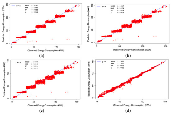
Figure 9.
Predicted EC vs. observed values on the test set with (a) RR model (); (b) LR model (); (c) ENR model (); and (d) WOA/MARS model ().
4. Conclusions
This study demonstrates the effectiveness of a WOA-tuned MARS model for estimating energy consumption in steel production, achieving exceptional predictive accuracy (R2 = 0.9972). The model’s superiority over linear alternatives (RR, LR, and ENR) stems from its ability to capture nonlinear interactions between critical process variables, which align with established steelmaking physics:
- CO2 emissions and energy consumption (EC) exhibit a strong coupling due to shared dependencies on production volume and combustion intensity.
- Lagging reactive power (LaCRP) reflects inductive load dominance, where a poor power factor increases the apparent power demand and, thus, EC.
- Lagging current power factor (LaCPF) extremes indicate suboptimal electrical efficiency, correlating with higher energy losses.
In conclusion, the WOA-tuned MARS model presents a robust methodology for estimating electrical energy consumption in the steel industry. Given the absence of analytical equations capable of accurately predicting steelworks’ electrical energy consumption (SEC) from experimental data alone, alternative diagnostic approaches become indispensable. This methodology demonstrates adaptability to a broad spectrum of manufacturing processes, though its implementation must account for the specific operational characteristics and conditions of individual steelworks.
Limitations and future work: While the proposed methodology demonstrates high accuracy, several limitations and opportunities for future research should be acknowledged:
- Dataset specificity: The current analysis focuses on data from Gwangyang Steelworks (South Korea). Future studies should validate the model’s generalizability across diverse geographical regions and steel plant configurations.
- External factors: Incorporating market demand fluctuations, regulatory changes, and seasonal variations could refine the model’s adaptability to dynamic industrial conditions.
- Temporal validation: Employing time-aware data splits (e.g., training on historical data and testing on recent periods) would further assess the model’s robustness to operational evolution.
- Potential methodological extensions include the following:
- Dynamic hyperparameter tuning using expanding/rolling window strategies to capture long-term trends.
- Hybrid approaches (e.g., MARS + ARIMA) to balance interpretability and predictive power for time-series forecasting.
Author Contributions
Conceptualization, P.J.G.-N., E.G.-G., L.A.M.-G., L.Á.-d.-P., M.M.-F. and A.B.-S.; methodology, P.J.G.-N., E.G.-G., L.A.M.-G., L.Á.-d.-P., M.M.-F. and A.B.-S.; software, P.J.G.-N., E.G.-G., L.A.M.-G., L.Á.-d.-P., M.M.-F. and A.B.-S.; validation, P.J.G.-N., E.G.-G., L.A.M.-G., L.Á.-d.-P., M.M.-F. and A.B.-S.; formal analysis, P.J.G.-N., E.G.-G., L.A.M.-G., L.Á.-d.-P., M.M.-F. and A.B.-S.; data curation, P.J.G.-N., E.G.-G., L.A.M.-G., L.Á.-d.-P., M.M.-F. and A.B.-S.; writing—original draft preparation, P.J.G.-N., E.G.-G., L.A.M.-G., L.Á.-d.-P., M.M.-F. and A.B.-S.; writing—review and editing, P.J.G.-N., E.G.-G., L.A.M.-G., L.Á.-d.-P., M.M.-F. and A.B.-S.; visualization, P.J.G.-N., E.G.-G., L.A.M.-G., L.Á.-d.-P., M.M.-F. and A.B.-S.; supervision, P.J.G.-N., E.G.-G., L.A.M.-G., L.Á.-d.-P., M.M.-F. and A.B.-S. All authors have read and agreed to the published version of the manuscript.
Funding
This research received no external funding.
Data Availability Statement
The data that support the findings of this study are available from the following link: https://archive.ics.uci.edu/dataset/851/steel+industry+energy+consumption (accessed on 15 April 2024).
Acknowledgments
The Mathematics Department at the University of Oviedo generously provided computational assistance. Likewise, the authors would like to thank Anthony Ashworth for revising this research paper in English.
Conflicts of Interest
The authors declare no competing interests.
References
- Xiao, L.; Shao, W.; Liang, T.; Wang, C. A Combined Model Based on Multiple Seasonal Patterns and Modified Firefly Algorithm for Electrical Load Forecasting. Appl. Energy 2016, 167, 135–153. [Google Scholar] [CrossRef]
- Conejo, A.N.; Birat, J.-P.; Dutta, A. A Review of the Current Environmental Challenges of the Steel Industry and Its Value Chain. J. Environ. Manag. 2020, 259, 109782. [Google Scholar] [CrossRef]
- Gogeri, I.; Gouda, K.C.; Sumathy, T. Modeling and Forecasting Atmospheric Carbon Dioxide Concentrations at Bengaluru City in India. Stoch. Environ. Res. Risk Assess. 2024, 38, 1297–1312. [Google Scholar] [CrossRef]
- Tian, W.; An, H.; Li, X.; Li, H.; Quan, K.; Lu, X.; Bai, H. CO2 Accounting Model and Carbon Reduction Analysis of Iron and Steel Plants Based on Intra- and Inter-Process Carbon Metabolism. J. Clean. Prod. 2022, 360, 132190. [Google Scholar] [CrossRef]
- Holappa, L. A General Vision for Reduction of Energy Consumption and CO2 Emissions from the Steel Industry. Metals 2020, 10, 1117. [Google Scholar] [CrossRef]
- González-Álvarez, M.A.; Montañés, A. CO2 Emissions, Energy Consumption, and Economic Growth: Determining the Stability of the 3E Relationship. Econ. Modell. 2023, 121, 106195. [Google Scholar] [CrossRef]
- Bai, H.; Lu, X.; Li, H.; Zhao, L.; Liu, X.; Li, N.; Wei, W.; Cang, D. The Relationship between Energy Consumption and CO2 Emissions in Iron and Steel Making. In Energy Technology 2012; Salazar-Villalpando, M.D., Neelameggham, N.R., Guillen, D.P., Pati, S., Krumdick, G.K., Eds.; Wiley: Hoboken, NJ, USA, 2012; pp. 125–132. ISBN 978-1-118-29138-2. [Google Scholar]
- Griffin, P.W.; Hammond, G.P. Industrial Energy Use and Carbon Emissions Reduction in the Iron and Steel Sector: A UK Perspective. Appl. Energy 2019, 249, 109–125. [Google Scholar] [CrossRef]
- Pardo, N.; Moya, J.; Vatapoulos, K. Prospective Scenarios on Energy Efficiency and CO2 Emissions in the EU Iron & Steel Industry; Publications Office of European Union, Institute for Energy and Transport: Luxembourg, 2015. [Google Scholar]
- Wang, Z.-X.; Li, Q.; Pei, L.-L. A Seasonal GM(1,1) Model for Forecasting the Electricity Consumption of the Primary Economic Sectors. Energy 2018, 154, 522–534. [Google Scholar] [CrossRef]
- Candanedo, L.M.; Feldheim, V.; Deramaix, D. Data Driven Prediction Models of Energy Use of Appliances in a Low-Energy House. Energy Build. 2017, 140, 81–97. [Google Scholar] [CrossRef]
- Le, T.; Zhao, J. A Data Fusion Algorithm Based on Neural Network Research in Building Environment of Wireless Sensor Network. Int. J. Future Gener. Commun. Netw. 2015, 8, 295–306. [Google Scholar] [CrossRef]
- Alsharif, M.H.; Younes, M.K.; Kim, J. Time Series ARIMA Model for Prediction of Daily and Monthly Average Global Solar Radiation: The Case Study of Seoul, South Korea. Symmetry 2019, 11, 240. [Google Scholar] [CrossRef]
- Lv, J.; Li, X.; Ding, L.; Jiang, L. Applying Principal Component Analysis and Weighted Support Vector Machine in Building Cooling Load Forecasting. In Proceedings of the 2010 International Conference on Computer and Communication Technologies in Agriculture Engineering, Chengdu, China, 12–13 June 2010; pp. 434–437. [Google Scholar]
- Amiri, S.S.; Mottahedi, M.; Asadi, S. Using Multiple Regression Analysis to Develop Energy Consumption Indicators for Commercial Buildings in the U.S. Energy Build. 2015, 109, 209–216. [Google Scholar] [CrossRef]
- Mocanu, E.; Nguyen, P.H.; Gibescu, M.; Kling, W.L. Deep Learning for Estimating Building Energy Consumption. Sustain. Energy Grids Netw. 2016, 6, 91–99. [Google Scholar] [CrossRef]
- Sathishkumar, V.E.; Shin, C.; Cho, Y. Efficient Energy Consumption Prediction Model for a Data Analytic-Enabled Industry Building in a Smart City. Build. Res. Inf. 2021, 49, 127–143. [Google Scholar] [CrossRef]
- Friedman, J.H. Multivariate Adaptive Regression Splines. Ann. Statist 1991, 19, 1–67. [Google Scholar] [CrossRef]
- Kooperberg, C. Multivariate Adaptive Regression Splines. In Wiley StatsRef: Statistics Reference Online; Kenett, R.S., Longford, N.T., Piegorsch, W.W., Ruggeri, F., Eds.; Wiley: Boca Raton, FL, USA, 2014; ISBN 978-1-118-44511-2. [Google Scholar]
- Lange, C. Practical Machine Learning with R: Tutorials and Case Studies, 1st ed.; CRC Press LLC: Abingdon, UK, 2024; ISBN 978-1-040-02124-8. [Google Scholar]
- Marsland, S. Machine Learning: An Algorithmic Perspective, 2nd ed.; CRC Press, Taylor and Francis Group: Boca Raton, FL, USA, 2015; ISBN 978-1-4665-8333-7. [Google Scholar]
- Murphy, K.P. Machine Learning: A Probabilistic Perspective; Adaptive Computation and Machine Learning Series; MIT Press: Cambridge, MA, USA, 2012; ISBN 978-0-262-01802-9. [Google Scholar]
- Sekulic, S.; Kowalski, B.R. MARS: A Tutorial. J. Chemom. 1992, 6, 199–216. [Google Scholar] [CrossRef]
- Vidoli, F. Evaluating the Water Sector in Italy through a Two Stage Method Using the Conditional Robust Nonparametric Frontier and Multivariate Adaptive Regression Splines. Eur. J. Oper. Res. 2011, 212, 583–595. [Google Scholar] [CrossRef]
- Xu, Q.-S.; Daszykowski, M.; Walczak, B.; Daeyaert, F.; De Jonge, M.R.; Heeres, J.; Koymans, L.M.H.; Lewi, P.J.; Vinkers, H.M.; Janssen, P.A.; et al. Multivariate Adaptive Regression Splines—Studies of HIV Reverse Transcriptase Inhibitors. Chemom. Intell. Lab. Syst. 2004, 72, 27–34. [Google Scholar] [CrossRef]
- Ebrahimgol, H.; Aghaie, M.; Zolfaghari, A.; Naserbegi, A. A Novel Approach in Exergy Optimization of a WWER1000 Nuclear Power Plant Using Whale Optimization Algorithm. Ann. Nucl. Eng. 2020, 145, 107540. [Google Scholar] [CrossRef]
- Huang, K.-W.; Wu, Z.-X.; Jiang, C.-L.; Huang, Z.-H.; Lee, S.-H. WPO: A Whale Particle Optimization Algorithm. Int. J. Comput. Intell. Syst. 2023, 16, 115. [Google Scholar] [CrossRef]
- Mirjalili, S.; Lewis, A. The Whale Optimization Algorithm. Adv. Eng. Softw. 2016, 95, 51–67. [Google Scholar] [CrossRef]
- Onwubolu, G.C.; Babu, B.V. New Optimization Techniques in Engineering; Studies in Fuzziness and Soft Computing; Springer: Berlin/Heidelberg, Germany, 2004; Volume 141, ISBN 978-3-642-05767-0. [Google Scholar]
- Zheng, G.; Zhang, W.; Zhou, H.; Yang, P. Multivariate Adaptive Regression Splines Model for Prediction of the Liquefaction-Induced Settlement of Shallow Foundations. Soil Dyn. Earthq. Eng. 2020, 132, 106097. [Google Scholar] [CrossRef]
- Kuhn, M.; Johnson, K. Applied Predictive Modeling; Springer: New York, NY, USA, 2013; ISBN 978-1-4614-6848-6. [Google Scholar]
- Izenman, A.J. Modern Multivariate Statistical Techniques; Springer Texts in Statistics; Springer: New York, NY, USA, 2008; ISBN 978-0-387-78188-4. [Google Scholar]
- Keeney, A.J.; Beseler, C.L.; Ingold, S.S. County-Level Analysis on Occupation and Ecological Determinants of Child Abuse and Neglect Rates Employing Elastic Net Regression. Child Abus. Negl. 2023, 137, 106029. [Google Scholar] [CrossRef] [PubMed]
- Saleh, A.K.M.E.; Arashi, M.; Kibria, B.M.G. Theory of Ridge Regression Estimation with Applications; Wiley: Hoboken, NJ, USA, 2019; ISBN 978-1-118-64447-8. [Google Scholar]
- Zhang, L.; Tedde, A.; Ho, P.; Grelet, C.; Dehareng, F.; Froidmont, E.; Gengler, N.; Brostaux, Y.; Hailemariam, D.; Pryce, J.; et al. Mining Data from Milk Mid-Infrared Spectroscopy and Animal Characteristics to Improve the Prediction of Dairy Cow’s Liveweight Using Feature Selection Algorithms Based on Partial Least Squares and Elastic Net Regressions. Comput. Electron. Agric. 2021, 184, 106106. [Google Scholar] [CrossRef]
- Rogers, S.; Girolami, M. A First Course in Machine Learning; Chapman and Hall/CRC: London, UK, 2016; ISBN 978-1-4987-3854-5. [Google Scholar]
- Vapnik, V.N. Statistical Learning Theory; Adaptive and Learning Systems for Signal Processing, Communications, and Control; Wiley: New York, NY, USA; Weinheim, Germany, 1998; ISBN 978-0-471-03003-4. [Google Scholar]
- Gackowski, M.; Szewczyk-Golec, K.; Pluskota, R.; Koba, M.; Mądra-Gackowska, K.; Woźniak, A. Application of Multivariate Adaptive Regression Splines (MARSplines) for Predicting Antitumor Activity of Anthrapyrazole Derivatives. Int. J. Mol. Sci. 2022, 23, 5132. [Google Scholar] [CrossRef] [PubMed]
- De Benedetto, D.; Barca, E.; Castellini, M.; Popolizio, S.; Lacolla, G.; Stellacci, A.M. Prediction of Soil Organic Carbon at Field Scale by Regression Kriging and Multivariate Adaptive Regression Splines Using Geophysical Covariates. Land 2022, 11, 381. [Google Scholar] [CrossRef]
- Majeed, F.; Ziggah, Y.Y.; Kusi-Manu, C.; Ibrahim, B.; Ahenkorah, I. A Novel Artificial Intelligence Approach for Regolith Geochemical Grade Prediction Using Multivariate Adaptive Regression Splines. Geosystems Geoenvironment 2022, 1, 100038. [Google Scholar] [CrossRef]
- Agwu, O.E.; Elraies, K.A.; Alkouh, A.; Alatefi, S. Mathematical Modelling of Drilling Mud Plastic Viscosity at Downhole Conditions Using Multivariate Adaptive Regression Splines. Geoenergy Sci. Eng. 2024, 233, 212584. [Google Scholar] [CrossRef]
- Sharma, J.; Kumar Mitra, S. Developing a Used Car Pricing Model Applying Multivariate Adaptive Regression Splines Approach. Expert Syst. Appl. 2024, 236, 121277. [Google Scholar] [CrossRef]
- Menéndez García, L.A.; Sánchez Lasheras, F.; García Nieto, P.J.; Álvarez De Prado, L.; Bernardo Sánchez, A. Predicting Benzene Concentration Using Machine Learning and Time Series Algorithms. Mathematics 2020, 8, 2205. [Google Scholar] [CrossRef]
- Ali, H.M.; Mohammadi Ghaleni, M.; Moghaddasi, M.; Moradi, M. A Novel Interpretable Hybrid Model for Multi-Step Ahead Dissolved Oxygen Forecasting in the Mississippi River Basin. Stoch. Environ. Res. Risk Assess. 2024, 38, 4629–4656. [Google Scholar] [CrossRef]
- Sathishkumar, V.E.; Lim, J.; Lee, M.; Cho, K.; Park, J.; Shin, C.; Cho, Y. Steel Industry Energy Consumption. 2021. Available online: https://archive.ics.uci.edu/dataset/851/steel+industry+energy+consumption (accessed on 15 April 2024).
- Sathishkumar, V.E.; Lim, J.; Lee, M.; Cho, K.; Park, J.; Shin, C. Industry Energy Consumption Prediction Using Data Mining Techniques. Int. J. Energy Inf. Commun. 2020, 11, 7–14. [Google Scholar] [CrossRef]
- Dutta, S.K.; Chokshi, Y.B. Basic Concepts of Iron and Steel Making; Springer: Singapore, 2020; ISBN 978-981-15-2436-3. [Google Scholar]
- Bishop, C.M. Pattern Recognition and Machine Learning; Information science and statistics; Springer: New York, NY, USA, 2006; ISBN 978-0-387-31073-2. [Google Scholar]
- Smith, C. Decision Trees and Random Forests: A Visual Introduction for Beginners; Blue Windmill Media: Thornton, ON, Canada, 2017; ISBN 978-1-5498-9375-9. [Google Scholar]
- Qureshi, M.U.; Mahmood, Z.; Rasool, A.M. Using Multivariate Adaptive Regression Splines to Develop Relationship between Rock Quality Designation and Permeability. J. Rock Mech. Geotech. Eng. 2022, 14, 1180–1187. [Google Scholar] [CrossRef]
- Verma, V.K.; Banodha, U.; Malpani, K. Optimization with Adaptive Learning: A Better Approach for Reducing SSE to Fit Accurate Linear Regression Model for Prediction. Int. J. Adv. Comput. Sci. Appl. 2024, 15, 168. [Google Scholar] [CrossRef]
- Faraway, J.J. Linear Models with R, 2nd ed.; Texts in Statistical Science; CRC Press: Boca Raton, FL, USA, 2014; ISBN 978-1-4398-8734-9. [Google Scholar]
- Thijssen, J.J.J. A Concise Introduction to Statistical Inference; CRC Press: Boca Raton, FL, USA, 2017; ISBN 978-1-4987-5578-8. [Google Scholar]
- Henderson, S.; Royall, K.E. Barrow Steelworks—Continuous Casting; Stanley Henderson: Los Angeles, CA, USA, 2021; ISBN 978-1-913898-24-3. [Google Scholar]
- Jung, Y. Multiple Predicting K-Fold Cross-Validation for Model Selection. J. Nonparametr. Stat. 2018, 30, 197–215. [Google Scholar] [CrossRef]
- Agresti, A.; Kateri, M. Foundations of Statistics for Data Scientists: With R and Python; Chapman & Hall/CRC Texts in Statistical Science; CRC Press: Boca Raton, FL, USA, 2021; ISBN 978-1-000-46293-7. [Google Scholar]
- Milborrow, S. Earth: Multivariate Adaptive Regression Splines; R Package; 2023. Available online: https://cran.r-project.org/web/packages/earth/earth.pdf (accessed on 5 October 2024).
- Tay, J.K.; Narasimhan, B.; Hastie, T. Elastic Net Regularization Paths for All Generalized Linear Models. J. Stat. Soft. 2023, 106, 1–31. [Google Scholar] [CrossRef]
- Mubarak, H.; Sanjari, M.J.; Stegen, S.; Abdellatif, A. Improved Active and Reactive Energy Forecasting Using a Stacking Ensemble Approach: Steel Industry Case Study. Energies 2023, 16, 7252. [Google Scholar] [CrossRef]
- Deisenroth, M.P.; Faisal, A.A.; Ong, C.S. Mathematics for Machine Learning; Cambridge University Press: Cambridge, UK, 2020; ISBN 978-1-108-47004-9. [Google Scholar]
- Pan, S.-Y.; Chang, E.E.; Chiang, P.-C. CO2 Capture by Accelerated Carbonation of Alkaline Wastes: A Review on Its Principles and Applications. Aerosol Air Qual. Res. 2012, 12, 770–791. [Google Scholar] [CrossRef]
- Maarif, M.R.; Saleh, A.R.; Habibi, M.; Fitriyani, N.L.; Syafrudin, M. Energy Usage Forecasting Model Based on Long Short-Term Memory (LSTM) and eXplainable Artificial Intelligence (XAI). Information 2023, 14, 265. [Google Scholar] [CrossRef]
- Turkovskyi, V.; Malinovskyi, A.; Muzychak, A.; Turkovskyi, O. Using the Constant Current—Constant Voltage Converters to Effectively Reduce Voltage Fluctuations in the Power Supply Systems for Electric Arc Furnaces. East.-Eur. J. Enterp. Technol. 2020, 6, 54–63. [Google Scholar] [CrossRef]
- Sizirici, B.; Fseha, Y.; Cho, C.-S.; Yildiz, I.; Byon, Y.-J. A Review of Carbon Footprint Reduction in Construction Industry, from Design to Operation. Materials 2021, 14, 6094. [Google Scholar] [CrossRef] [PubMed]
- Perpiñán, J.; Bailera, M.; Romeo, L.; Peña, B.; Eveloy, V. CO2 Recycling in the Iron and Steel Industry via Power-to-Gas and Oxy-Fuel Combustion. Energies 2021, 14, 7090. [Google Scholar] [CrossRef]


Disclaimer/Publisher’s Note: The statements, opinions and data contained in all publications are solely those of the individual author(s) and contributor(s) and not of MDPI and/or the editor(s). MDPI and/or the editor(s) disclaim responsibility for any injury to people or property resulting from any ideas, methods, instructions or products referred to in the content. |
© 2025 by the authors. Licensee MDPI, Basel, Switzerland. This article is an open access article distributed under the terms and conditions of the Creative Commons Attribution (CC BY) license (https://creativecommons.org/licenses/by/4.0/).