Abstract
This paper proposes a numerical algorithm for the nonlinear fifth-order Korteweg–de Vries equations. This class of equations is known for its significance in modeling various complex wave phenomena in physics and engineering. The approximate solutions are expressed in terms of certain shifted Horadam polynomials. A theoretical background for these polynomials is first introduced. The derivatives of these polynomials and their operational metrics of derivatives are established to tackle the problem using the typical collocation method to transform the nonlinear fifth-order Korteweg–de Vries equation governed by its underlying conditions into a system of nonlinear algebraic equations, thereby obtaining the approximate solutions. This paper also includes a rigorous convergence analysis of the proposed shifted Horadam expansion. To validate the proposed method, we present several numerical examples illustrating its accuracy and effectiveness.
Keywords:
generalized Fibonacci polynomials; Korteweg–de Vries equations; operational matrices; convergence analysis; collocation method MSC:
33C45; 65M70; 35Q53
1. Introduction
Nonlinear differential equations (DEs) are vital since they can represent complicated real-world phenomena in numerous fields of science and engineering branches. Complex systems can be better understood by studying nonlinear DEs, which, in contrast to linear ones, can display a wide range of behaviors. These behaviors include multistability, chaos, and bifurcations. Many models in different disciplines, such as electrodynamics, neuroscience, epidemiology, mechanical engineering, fluid dynamics, and economics, can be modeled using nonlinear DEs; see, for example, [1,2,3]. Since most of these models lack exact solutions, numerical methods are crucial in treating these nonlinear DEs. For example, the authors of [4] followed a numerical approach for treating the Black–Scholes model. The authors of [5] used a collocation approach to solve the Fitzhugh–Nagumo nonlinear DEs in neuroscience. Another numerical approach was followed in [6] to solve the nonlinear equations of Emden–Fowler models. Nonlinear thermal diffusion problems were handled in [7]. In [8], a numerical scheme for solving a stochastic nonlinear advection-diffusion dynamical model was handled. In [9], the authors employed Petrov-Galerkin methods for treating some linear and nonlinear partial DEs. The authors of [10] used a specific difference scheme for some nonlinear fractional DEs. The authors of [11] a collocation procedure for treating the nonlinear fractional FitzHugh–Nagumo equation.
An important nonlinear partial differential equation that describes the motion of solitons (individual waves) in shallow water and other systems is the Korteweg–de Vries (KdV) equation. Over the years, the KdV equation has undergone several revisions to account for non-local interactions, dissipation effects, higher-order terms, and various physical phenomena. Many scientific fields have used these modifications; nonlinear optics, fluid dynamics, and plasma physics are just a few examples. The following are a few notable variations of the KdV equation and the several scientific domains that have used them: the standard KdV equations, the modified KdV equation, the generalized KdV equation, the KdV–Burgers equation, and the KdV–Kawahara equation. Furthermore, regarding some applications of some specific problems of the KdV-type equations, we mention three of these problems and their applications.
- The Caudrey–Dodd–Gibbon problem. This problem has applications in shallow water waves, nonlinear optics, and plasma physics; see [12].
- The Sawada–Kotera problem has applications in hydrodynamics, elasticity, plasma physics, and soliton theory; see [13].
- The Kaup-Kuperschmidt problem has applications in fluid mechanics, biological wave propagation, plasma physics, and quantum field theory; see [14].
Numerous contributions have focused on their handling due to the significance of the various KdV-type equations. For example, in [15], analytical and numerical solutions for the fifth-order KdV equation were presented. In [16], some hyperelliptic solutions of certain modified KdV equations were proposed. A numerical study for the stochastic KdV equation was presented in [17]. To treat the generalized Kawahara equation, an operational matrix approach was proposed in [18]. The authors of [19] followed a finite difference approach to handle the fractional KdV equation. Two algorithms were presented in [20] to treat the nonlinear time-fractional Lax’s KdV equation. Another numerical approach was given in [21] for approximating the modified KdV equation. A computational approach was used to handle a higher-order KdV equation in [22]. The time-fractional KdV equation was investigated numerically in [23]. In [24], the method of lines was proposed to solve the KdV equation. A Bernstein polynomial basis was employed in [25] to treat the KdV-type equations.
Special functions are fundamental in the scientific, mathematical, and engineering fields. For examples of the usage of these polynomials in signal processing, quantum mechanics, and physics, one can consult [26,27]. These functions have the potential to solve several types of DEs. For example, the authors of [28] numerically treated the fractional Rayleigh-Stokes problem using certain orthogonal combinations of Chebyshev polynomials. The shifted Fibonacci polynomials were utilized in [29] to treat the fractional Burgers equation. In [30], the authors used Vieta–Fibonacci polynomials to treat certain two-dimensional problems. Other two-dimensional FDEs were handled using Vieta Lucas polynomials in [31]. The authors of [32] used Changhee polynomials to treat a high-dimensional chaotic Lorenz system. In [33], some FDEs were treated using shifted Chebyshev polynomials.
Horadam sequences, named after the mathematician Alwyn Horadam, who initially developed them in the 1960s, generalize several well-known polynomials, such as Fibonacci, Lucas, Pell, and Pell Lucas polynomials. Many authors investigated Horadam sequences of polynomials. For example, the authors in [34] investigated some generalized Horadam polynomials and numbers. Some identities regarding Horadam sequences were developed in [35]. Some subclasses of bi-univalent functions associated with the Horadam polynomials were given in [36]. In [37], some characterizations of periodic generalized Horadam sequences were introduced. An application to specific Horadam sequences in coding theory was presented in [38].
Spectral methods are becoming essential in the applied sciences; see, for instance [39,40], for some of their applications in fields like engineering and fluid dynamics. These methods involve approximating differential and integral equation solutions by expansions of various special functions. The three spectral techniques most frequently employed are the collocation, tau, and Galerkin methods. The type of differential equation and the boundary conditions it governs determine which spectral method is suitable. The three spectral approaches use different trial and test functions. The Galerkin approach selects all basis function members to satisfy the underlying conditions imposed by a specific differential equation, treating the test and trial functions as equivalent. (For a few references, see [41,42,43].) The tau method is easier than the Galerkin method in application since there are no restrictions on selecting the trial and test functions; see, for example, [44,45,46]. The collocation method is the most popular spectral method because it works well with nonlinear DEs and can be used with all kinds of DEs, no matter what the underlying conditions are; see, for example, [47,48,49,50].
We comment here that the motivations for our work are as follows:
- KdV-type equations are among the most important problems encountered in applied sciences, which motivates us to investigate them using a new approach.
- Several spectral approaches were followed to solve KdV-type equations with various orthogonal polynomials as basis functions. The basis functions used in this article are a family of polynomials that are not orthogonal. This article will motivate us to apply these polynomials to other problems in the applied sciences.
- To the best of our knowledge, the specific Horadam sequence of polynomials used in this paper was not previously used in numerical analysis, which provides a compelling reason to introduce and utilize them.
Furthermore, the work’s novelty is due to the following points:
- We have developed novel simplified formulas for the new sequence of polynomials, including their high-order derivatives and operational matrices of derivatives.
- This paper presents a new comprehensive study on the convergence analysis of the used Horadam expansion.
The main objectives of this paper can be listed in the following items:
- (a)
- Introducing a class of shifted Horadam polynomials and developing new essential formulas concerned with them.
- (b)
- Developing operational matrices of derivatives of the introduced shifted polynomials.
- (c)
- Analyzing a collocation procedure for solving the nonlinear fifth-order KdV equations.
- (d)
- Investigating the convergence analysis of the proposed Horadam expansion.
- (e)
- Verifying our numerical algorithm by presenting some illustrative examples.
This paper is structured as follows: Section 2 gives an overview of Horadam polynomials, their representation, and some particular polynomials of them. Section 3 introduces certain shifted Horadam polynomials and develops some theoretical formulas that will be used to design our numerical algorithm. Section 4 presents a collocation approach for treating the nonlinear fifth-order KdV-type equations. Section 5 discusses the convergence and error analysis of the proposed expansion in more detail. Section 6 presents some illustrative examples and comparisons. Finally, some discussions are given in Section 7.
2. An Overview of Horadam Polynomials and Some Particular Polynomials
Horadam presented a set of generalized polynomials in his seminal work [51]. These polynomials may be generated using the following recursive formula:
The polynomials can be written in the following Binet’s form:
The above sequence of polynomials generalizes some well-known polynomials, such as Fibonacci, Pell, Lucas, and Pell–Lucas polynomials.
The standard Fibonacci polynomials can be generated with the following recursive formula:
The standard Fibonacci polynomials, which are special ones of Horadam polynomials, have several extensions. The generalized Fibonacci polynomials are one example of such a generalization; they are derived using the following recursive formula:
It is worth noting here that for every k, is of degree k. These polynomials involve many celebrated sequences, such as Fibonacci, Pell, Fermat, and Chebyshev polynomials of the second kind. More precisely, we have the following expressions:
Recently, the authors of [29] have developed some new formulas for the shifted Fibonacci polynomials, defined as
In addition; they used these polynomials to solve the fractional Burgers’ equation. This paper will introduce specific polynomials of the shifted generalized Fibonacci polynomials, defined as
Note that for every , is of degree m.
The following formula is used to generate these polynomials:
The following section introduces fundamental formulas concerning the introduced polynomials .
3. Some New Formulas Concerned with the Introduced Shifted Polynomials
We will develop new formulas for the specific shifted Horadam polynomials defined in (7). The following two lemmas will present the power form representation and inversion formula for these polynomials, which are pivotal in this paper. Next, we will establish new derivative expressions for these polynomials and their operational matrices of derivatives.
3.1. Analytic Form and Its Inversion Formula
Theorem 1.
Let m be a non-negative integer. The power form representation of is given by
Proof.
Theorem 2.
Consider a non-negative integer m. The following inversion formula is valid:
Proof.
We prove Formula (14) by induction. The formula holds for . Assume the validity of (14), and we have to show the following formula:
Now, if we multiply Formula (14) by x, and make use of the recursive formula (8) in the following form:
then the following formula can be obtained:
which can be turned after some algebraic computations into the following form:
This completes the proof. □
3.2. Derivative Expressions and Operational Matrices of Derivatives of
Based on Theorems 1 and 2, an expression for the high-order derivatives of in terms of their original polynomials can be deduced. The following theorem exhibits this expression.
Theorem 3.
Consider two positive integers with . We have
where
with
Proof.
The analytic form of in (9) enables one to write as
The inversion formula in (14) converts the above formula into the following one:
The last formula can be rearranged to be written in a more convenient form:
Now, to obtain a simplified formula for the derivatives , we use symbolic algebra to find a closed form for the second sum that appears in the right-hand side of (22). For this purpose, we set
and use Zeilberger’s algorithm [52] to show that the following recursive formula is satisfied by :
with the following initial values:
which can be solved to obtain
and accordingly, Formula (22) reduces into the following one:
The last formula can be written in the following alternative form:
with
This finalizes the proof of Theorem 3. □
The following four corollaries exhibit the first-, second-, third-, and fifth-order derivatives of the polynomials . They are all consequences of Theorem 3.
Corollary 1.
The first derivative of can be expressed in the following form:
where
Corollary 2.
The second derivative of can be expressed in the following form:
where
Corollary 3.
The third derivative of can be expressed in the following form:
where
Corollary 4.
The fifth derivative of can be expressed in the following form:
where
Proof.
The proof of Corollaries 1–4 can be easily obtained after putting respectively in Theorem 3. □
The following corollary presents the operational matrices of the integer derivatives of the polynomials , which can be deduced from the above four corollaries.
Corollary 5.
If we consider the following vector:
then, the first-, second-, third-, and fifth-order derivatives of the vector can be written in the following matrix forms:
where , , , and are the operational matrices of derivatives of order .
Proof.
The expressions in (35) are direct consequences of Corollaries 1–4. □
4. A Collocation Approach for the Nonlinear Fifth-Order KdV-Type Partial DEs
Consider the following nonlinear fifth-order KdV-type partial differential equation [53,54]:
governed by the following initial and boundary conditions:
where are arbitrary constants.
Now, consider the following space:
Consequently, it can be assumed that any function can be represented as
where is the vector defined in (34), and is the matrix of unknowns, whose order is .
Now, we can write the residual of Equation (36) as
Thanks to Corollary 5 along with the expansion (41), the following expressions for the terms and , can be obtained:
By virtue of the expressions (43)–(47), the residual can be written in the following form:
Now, to obtain the expansion coefficients , we apply the spectral collocation method by forcing the residual to be zero at some collocation points , as follows:
Moreover, the initial and boundary conditions (37)–(39) imply the following equations:
The nonlinear system of equations formed by the equations in (50)–(55) and (49) may be solved with the use of a numerical solver, such as Newton’s iterative technique, and thus the approximate solution given by (41) can be found.
5. The Convergence and Error Analysis
This section provides a detailed convergence analysis of the proposed approximate expansion. To begin this study, specific inequalities are necessary.
Lemma 1.
The following inequality holds [55]:
where is the modified Bessel function of order n of the first kind.
Lemma 2.
Consider the infinitely differentiable function at the origin. can be expanded as
Proof.
Consider the following expansion for :
As a result of the inversion formula (14), the previous expansion transforms into the following form:
Now, expanding the right-hand side of the last equation and rearranging the similar terms, the following expansion can be obtained:
This completes the proof of this lemma. □
Lemma 3.
Consider any non-negative integer m. The following inequality holds for :
Proof.
Using the analytic form for in (9), we can write
Now, we will use the symbolic algebra to find a closed formula for the summation in (62). Set
Zeilberger’s algorithm [52] aids in demonstrating that the following first-order recursive formula is satisfied by :
which can be immediately solved to give
and this implies the following inequality:
Now, it is easy to see from (62) along with the inequality (63), that
This proves Lemma 3. □
Theorem 4.
If is defined on and where μ is a positive constant and , then we obtain
Moreover, the series converges absolutely.
Proof.
Based on Lemma 2 and the assumptions of the theorem, we can write
The application of Lemma 1 enables us to write the previous inequality as
which can be rewritten after simplifying the right-hand side of the last inequality as
We now show the second part of the theorem. Since we have
so the series converges absolutely. □
Theorem 5.
If satisfies the hypothesis of Theorem 4, and , then the following error estimation is satisfied:
Proof.
The definition of enables us to write
where denotes upper incomplete gamma functions [56]. □
Theorem 6.
Let , with and , where and are positive constants. One has
Moreover, the series converges absolutely.
Proof.
If we apply Lemma 2 and use the assumption , then we can write
If we use the assumptions: and , then we obtain
We obtain the desired result by performing similar steps as in the proof of Theorem 4. □
Theorem 7.
If satisfies the hypothesis of Theorem 6, then we have the following upper estimate on the truncation error:
Proof.
From definitions of η and we obtain
If Theorem 6 and Lemma 3 are applied, then the following inequalities can be obtained:
and accordingly, we obtain
This completes the proof of this theorem. □
6. Illustrative Examples
In this section, we present numerical examples to validate and demonstrate the applicability and accuracy of our proposed numerical algorithm. We also present comparisons with some other methods. Now, if we consider the successive errors and , then the order of convergence for the given method can be calculated as [57]
Example 1

([53,54]). Consider the following Lax equation of order five:
governed by
where the analytic solution of this problem is
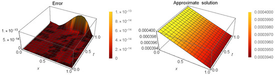
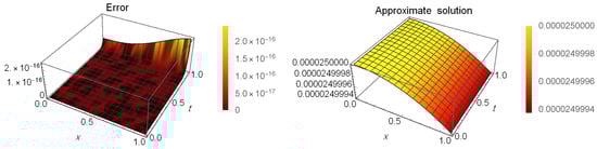
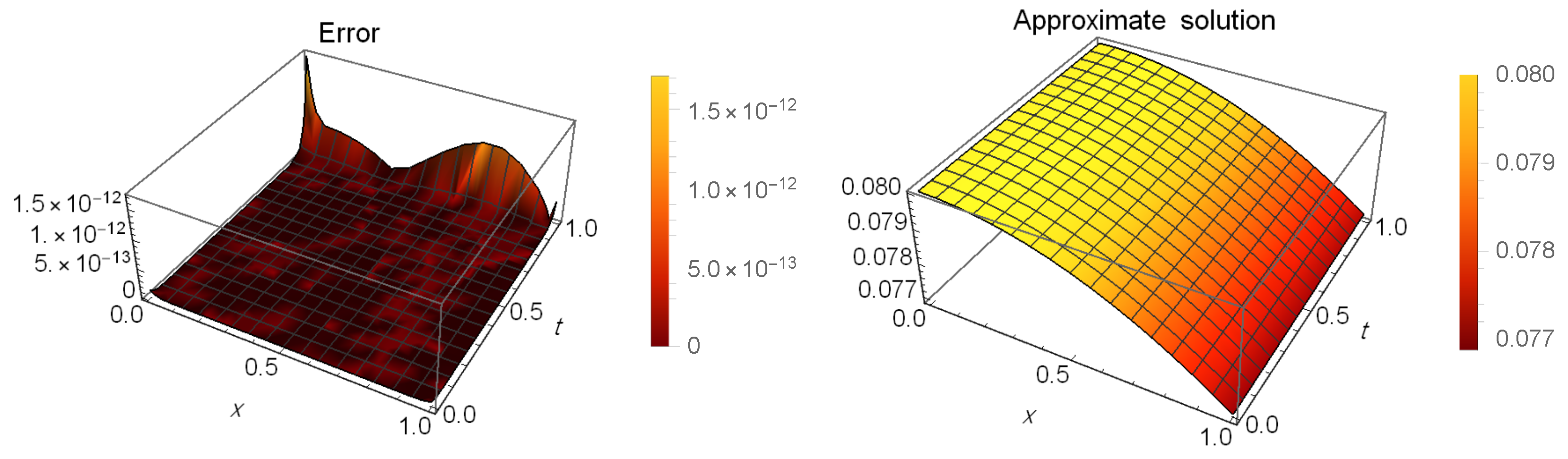
Table 1 presents a comparison of error between our method at and the method in [53] when and . Table 2 shows the CPU time used in seconds of the results in Table 1. Moreover, Table 3 shows the absolute errors (AEs) at different values of t when and . Table 4 shows the maximum AEs and the order of convergence, which is calculated by (81) at different values of N. Figure 1 illustrates the AEs (left) and approximate solution (right) at when and .
Table 1.
The error of Example 1.
Table 2.
CPU time used in seconds of Table 1.
Table 3.
The AEs of Example 1.
Table 4.
The maximum AEs and order of convergence for Example 1.
Figure 1.
The AEs and the approximate solution for Example 1.
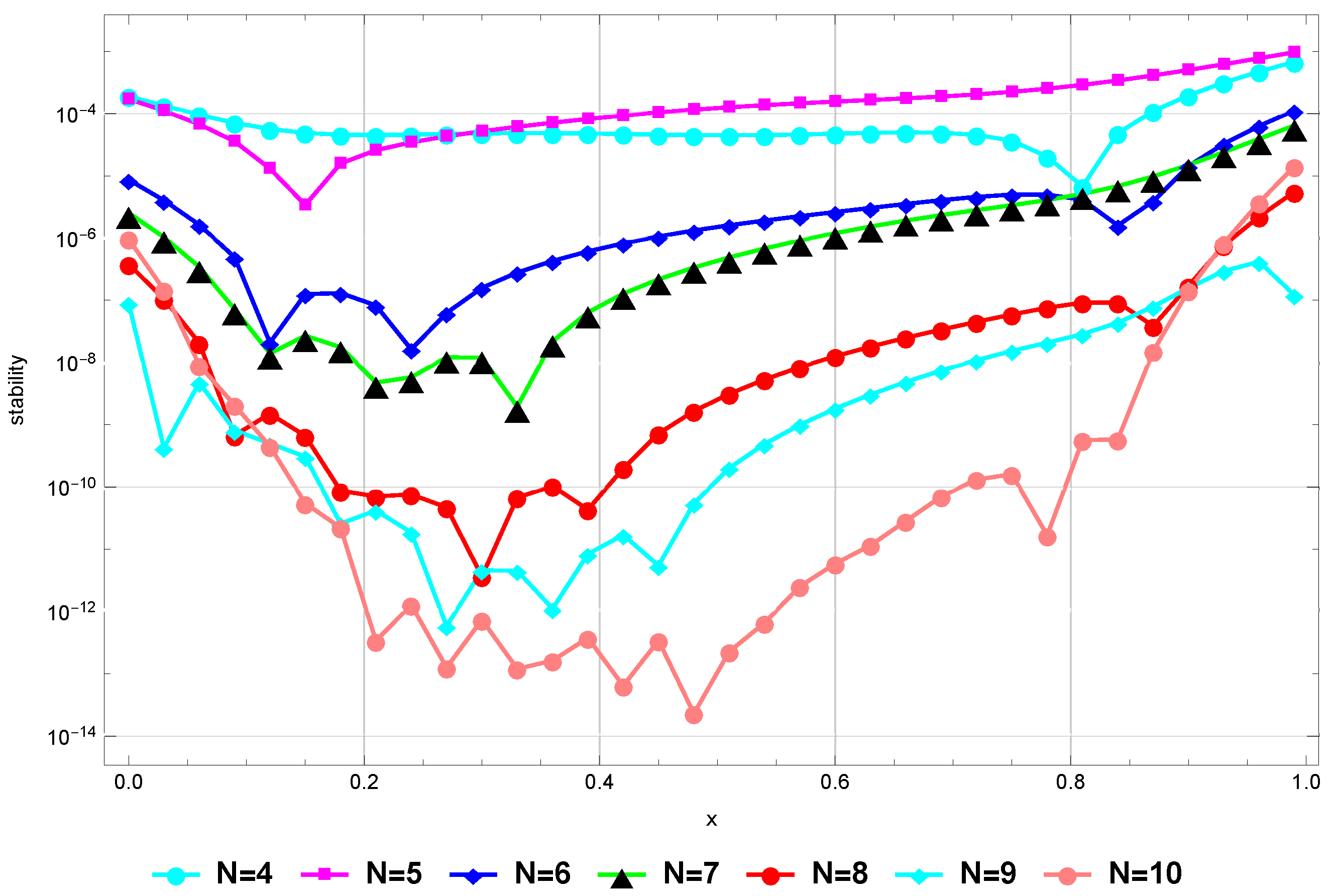
Remark 1
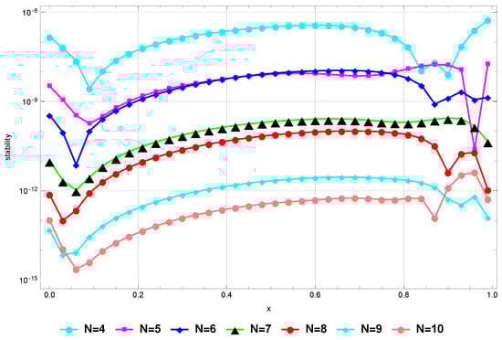
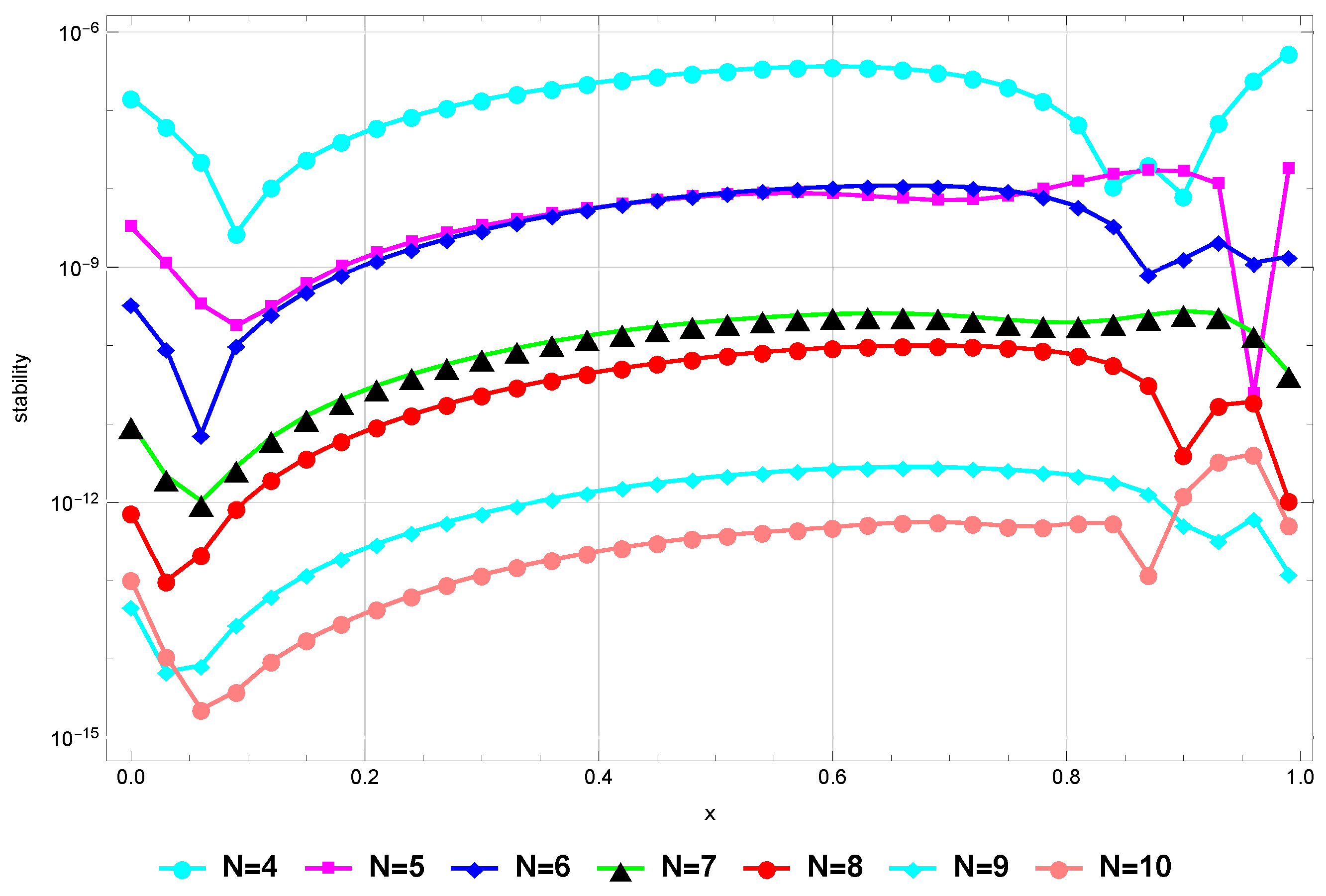
(Stability). We comment that our proposed method is stable in the sense that is sufficiently small for sufficiently large values of N, see [58]. To confirm this regarding Problem (82), we plot Figure 2 that shows that our method remains stable for .
Figure 2.
Stability for Example 1.
Remark 2
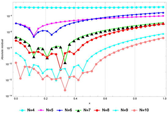
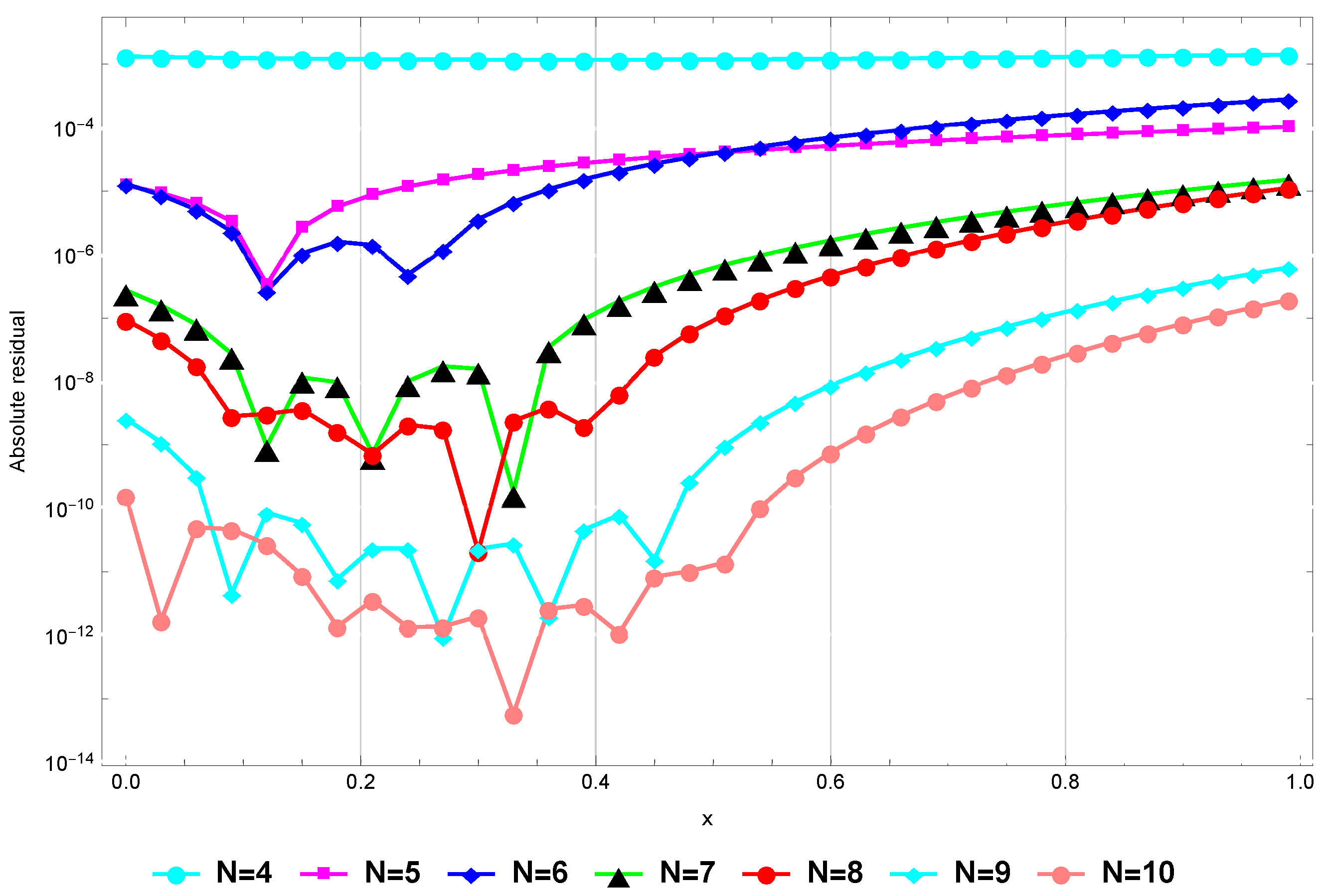
(Consistency). To show the consistency of our numerical method in the sense that is small for sufficiently large values of N, we plot Figure 3 that gives the absolute residual at for Problem (82). This figure shows the absolute residual at is sufficiently small for sufficiently large values of N.
Figure 3.
The absolute residual at for Example 1.
Example 2
([53,54]). Consider the following Sawada–Kotera equation of order five:
governed by
where the analytic solution of this problem is
Table 5 presents a comparison of error between our method at and the method in [53] when and . Table 6 shows the CPU time used in seconds of the results in Table 5. Moreover, Table 7 shows the AEs at different values of t when and . Figure 4 illustrates the AEs (left) and approximate solution (right) at when and .
Table 5.
The error of Example 2.
Table 6.
CPU time used in seconds of Table 5.
Table 7.
The AEs of Example 2.
Figure 4.
The AEs and the approximate solution for Example 2.
Example 3
([53,54]). Consider the following Caudrey–Dodd–Gibbon equation of order five:
governed by
where the analytic solution of this problem is
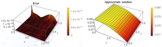
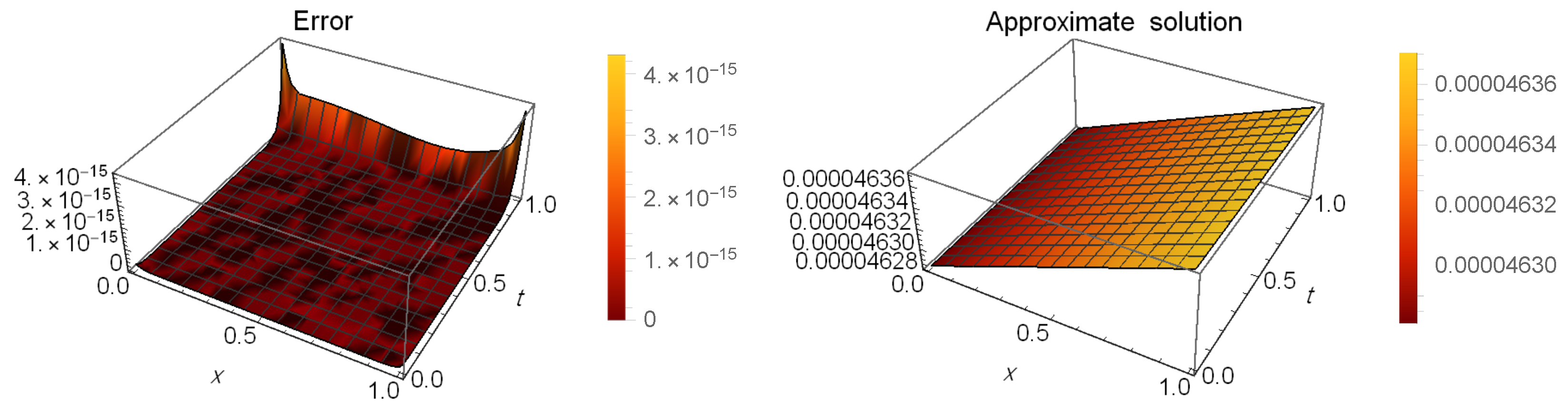
Table 8 presents a comparison of error between our method at and the method in [53] when . Table 9 shows the AEs at different values of t when . Figure 5 illustrates the AEs (left) and approximate solution (right) at when .
Table 8.
The error of Example 3.
Table 9.
The AEs of Example 3.
Figure 5.
The AEs and the approximate solution for Example 3.
Example 4

([53,54]). Consider the following fifth-order Kaup–Kuperschmidt equation:
governed by
where the analytic solution of this problem is
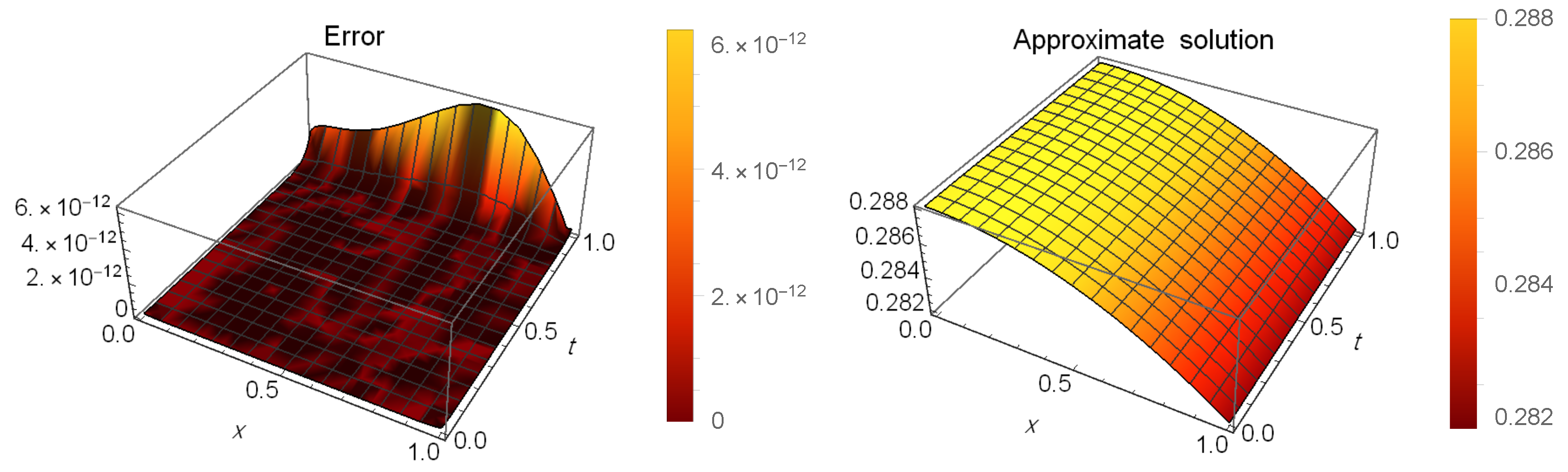
Table 10 presents a comparison of error between our method at , and the method in [53] when . Table 11 shows the AEs at different values of t when . Figure 6 illustrates the AEs (left) and approximate solution (right) at when .
Table 10.
The error of Example 4.
Table 11.
The AEs of Example 4.
Figure 6.
The AEs and the approximate solution for Example 4.
Example 5

([53,54]). Consider the following fifth-order Ito equation:
governed by
where the analytic solution of this problem is
Table 12 presents a comparison of error between our method at and the method in [53] when and . Table 13 shows the AEs at different values of t when and . Figure 7 illustrates the AEs (left) and approximate solution (right) at when and . Table 14 shows the maximum AEs and order of convergence (81) at different values of N.
Table 12.
The error of Example 5.
Table 13.
The AEs of Example 5.
Figure 7.
The AEs and the approximate solution for Example 5.
Table 14.
The maximum AEs and order of convergence for Example 5.
Remark 3.
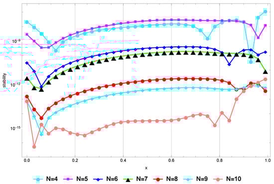
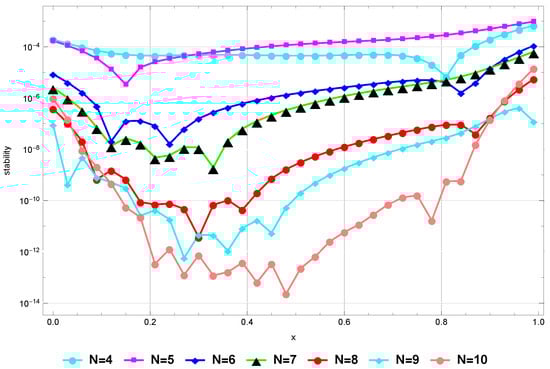
Figure 8 confirms that the method remains stable when for higher values of N. Finally, Figure 9 verifies that the at is sufficiently small for sufficiently large values of N, and this proves the consistency of the presented method.
Figure 8.
Stability for Example 5.
Figure 9.
The absolute residual at for Example 5.
Example 6.
Consider the following Sawada–Kotera equation of order five:
governed by
Since the exact solution is not available, so we define the following absolute residual error norm:
and applying the presented method at to obtain Table 15, which illustrates the RE.
Table 15.
The RE of Example 6.
7. Conclusions
This study successfully developed and analyzed a numerical algorithm to treat the fifth-order KdV-type equations, producing highly accurate results. The main idea was to introduce new shifted Horadam polynomials to act as basis functions. We established many basic formulas for these polynomials to design the proposed numerical method. In addition, some specific formulas and inequalities helped to investigate the convergence of the shifted Horadam approximate solutions in depth. We also offered numerical examples to confirm the method’s applicability and usefulness in tackling complicated nonlinear problems in mathematical physics and related domains. To the best of our knowledge, this is the first time these polynomials have been used in the scope of numerical solutions of DEs. We plan to employ these polynomials to treat other types of DEs in the applied sciences.
Author Contributions
Conceptualization, W.M.A.-E. and A.G.A.; Methodology, W.M.A.-E., O.M.A. and A.G.A.; Software, A.G.A.; Validation, W.M.A.-E., O.M.A. and A.G.A.; Formal analysis, W.M.A.-E. and A.G.A.; Investigation, W.M.A.-E., O.M.A. and A.G.A.; Writing—original draft, A.G.A. and W.M.A.-E.; Writing—review and editing, W.M.A.-E., A.G.A. and O.M.A.; Visualization, A.G.A. and W.M.A.-E.; Supervision, W.M.A.-E.; Funding acquisition, W.M.A.-E. and O.M.A. All authors have read and agreed to the published version of the manuscript.
Funding
This research received no external funding.
Data Availability Statement
Data are contained within the article.
Conflicts of Interest
The authors declare no conflicts of interest.
References
- Almatrafi, M.B.; Alharbi, A. New soliton wave solutions to a nonlinear equation arising in plasma physics. CMES-Comput. Model. Eng. Sci. 2023, 137, 827–841. [Google Scholar] [CrossRef]
- Parand, K.; Aghaei, A.A.; Kiani, S.; Zadeh, T.I.; Khosravi, Z. A neural network approach for solving nonlinear differential equations of Lane–Emden type. Eng. Comput. 2024, 40, 953–969. [Google Scholar] [CrossRef]
- Oruç, Ö. A new algorithm based on Lucas polynomials for approximate solution of 1D and 2D nonlinear generalized Benjamin–Bona–Mahony–Burgers equation. Comput. Math. Appl. 2017, 74, 3042–3057. [Google Scholar] [CrossRef]
- Bhowmik, S.K.; Khan, J.A. High-Accurate Numerical Schemes for Black–Scholes Models with Sensitivity Analysis. J. Math. 2022, 2022, 4488082. [Google Scholar] [CrossRef]
- Abd-Elhameed, W.M.; Al-Harbi, M.S.; Atta, A.G. New convolved Fibonacci collocation procedure for the Fitzhugh-Nagumo non-linear equation. Nonlinear Eng. 2024, 13, 20220332. [Google Scholar] [CrossRef]
- Mahdy, A.M.S. A numerical method for solving the nonlinear equations of Emden-Fowler models. J. Ocean Eng. Sci. 2022. [Google Scholar] [CrossRef]
- Majchrzak, E.; Mochnacki, B. The BEM application for numerical solution of non-steady and nonlinear thermal diffusion problems. Comput. Assist. Methods Eng. Sci. 2023, 3, 327–346. [Google Scholar]
- Yasin, M.W.; Iqbal, M.S.; Seadawy, A.R.; Baber, M.Z.; Younis, M.; Rizvi, S.T.R. Numerical scheme and analytical solutions to the stochastic nonlinear advection diffusion dynamical model. Int. J. Nonlinear Sci. Numer. Simul. 2023, 24, 467–487. [Google Scholar] [CrossRef]
- Shang, Y.; Wang, F.; Sun, J. Randomized neural network with Petrov–Galerkin methods for solving linear and nonlinear partial differential equations. Commun. Nonlinear Sci. Numer. Simul. 2023, 127, 107518. [Google Scholar] [CrossRef]
- Jiang, X.; Wang, J.; Wang, W.; Zhang, H. A predictor–corrector compact difference scheme for a nonlinear fractional differential equation. Fractal Fract. 2023, 7, 521. [Google Scholar] [CrossRef]
- Abd-Elhameed, W.M.; Alqubori, O.M.; Atta, A.G. A collocation procedure for treating the time-fractional FitzHugh–Nagumo differential equation using shifted Lucas polynomials. Mathematics 2024, 12, 3672. [Google Scholar] [CrossRef]
- Sadaf, M.; Arshed, S.; Akram, G.; Ahmad, M.; Abualnaja, K.M. Solitary dynamics of the Caudrey–Dodd–Gibbon equation using unified method. Opt. Quantum Electron. 2025, 57, 21. [Google Scholar] [CrossRef]
- Oad, A.; Arshad, M.; Shoaib, M.; Lu, D.; Li, X. Novel soliton solutions of two-mode Sawada-Kotera equation and its applications. IEEE Access 2021, 9, 127368–127381. [Google Scholar] [CrossRef]
- Alharthi, M.S. Extracting solitary solutions of the nonlinear Kaup–Kupershmidt (KK) equation by analytical method. Open Phys. 2023, 21, 20230134. [Google Scholar] [CrossRef]
- Attia, R.A.M.; Xia, Y.; Zhang, X.; Khater, M.M.A. Analytical and numerical investigation of soliton wave solutions in the fifth-order KdV equation within the KdV-KP framework. Results Phys. 2023, 51, 106646. [Google Scholar] [CrossRef]
- Matsutani, S. On real hyperelliptic solutions of focusing modified KdV equation. Math. Phys. Anal. Geom. 2024, 27, 19. [Google Scholar] [CrossRef]
- D’Ambrosio, R.; Di Giovacchino, S. Numerical conservation issues for the stochastic Korteweg–de Vries equation. J. Comput. Appl. Math. 2023, 424, 114967. [Google Scholar] [CrossRef]
- Ahmed, H.M.; Hafez, R.M.; Abd-Elhameed, W.M. A computational strategy for nonlinear time-fractional generalized Kawahara equation using new eighth-kind Chebyshev operational matrices. Phys. Scr. 2024, 99, 045250. [Google Scholar] [CrossRef]
- Dwivedi, M.; Sarkar, T. Fully discrete finite difference schemes for the fractional Korteweg-de Vries equation. J. Sci. Comput. 2024, 101, 30. [Google Scholar] [CrossRef]
- Mishra, N.K.; AlBaidani, M.M.; Khan, A.; Ganie, A.H. Two novel computational techniques for solving nonlinear time-fractional Lax’s Korteweg-de Vries equation. Axioms 2023, 12, 400. [Google Scholar] [CrossRef]
- Ahmad, F.; Rehman, S.U.; Zara, A. A new approach for the numerical approximation of modified Korteweg–de Vries equation. Math. Comput. Simul. 2023, 203, 189–206. [Google Scholar] [CrossRef]
- Haq, S.; Arifeen, S.U.; Noreen, A. An efficient computational technique for higher order KdV equation arising in shallow water waves. Appl. Numer. Math. 2023, 189, 53–65. [Google Scholar] [CrossRef]
- Cao, H.; Cheng, X.; Zhang, Q. Numerical simulation methods and analysis for the dynamics of the time-fractional KdV equation. Phys. D 2024, 460, 134050. [Google Scholar] [CrossRef]
- Alshareef, A.; Bakodah, H.O. Non-central m-point formula in method of lines for solving the Korteweg-de Vries (KdV) equation. J. Umm Al-Qura Univ. Appl. Sci. 2024, 1–11. [Google Scholar] [CrossRef]
- Ahmed, H.M. Numerical solutions of Korteweg-de Vries and Korteweg-de Vries-Burger’s equations in a Bernstein polynomial basis. Mediterr. J. Math. 2019, 16, 102. [Google Scholar] [CrossRef]
- Nikiforov, F.; Uvarov, V.B. Special Functions of Mathematical Physics; Springer: Berlin/Heidelberg, Germany, 1988; Volume 205. [Google Scholar]
- Shen, J.; Tang, T.; Wang, L.L. Spectral Methods: Algorithms, Analysis and Applications; Springer Science and Business Media: Berlin/Heidelberg, Germany, 2011; Volume 41. [Google Scholar]
- Abd-Elhameed, W.M.; Al-Sady, A.M.; Alqubori, O.M.; Atta, A.G. Numerical treatment of the fractional Rayleigh-Stokes problem using some orthogonal combinations of Chebyshev polynomials. AIMS Math. 2024, 9, 25457–25481. [Google Scholar] [CrossRef]
- Alharbi, M.H.; Abu Sunayh, A.F.; Atta, A.G.; Abd-Elhameed, W.M. Novel Approach by Shifted Fibonacci Polynomials for Solving the Fractional Burgers Equation. Fractal Fract. 2024, 8, 427. [Google Scholar] [CrossRef]
- Sharma, R.; Rajeev. An operational matrix approach to solve a 2D variable-order reaction advection diffusion equation with Vieta–Fibonacci polynomials. Spec. Top. Rev. Porous Media Int. J. 2023, 14, 79–96. [Google Scholar] [CrossRef]
- Sharma, R.; Rajeev. A numerical approach to solve 2D fractional RADE of variable-order with Vieta–Lucas polynomials. Chin. J. Phys. 2023, 86, 433–446. [Google Scholar] [CrossRef]
- Adel, M.; Khader, M.M.; Algelany, S. High-dimensional chaotic Lorenz system: Numerical treatment using Changhee polynomials of the Appell type. Fractal Fract. 2023, 7, 398. [Google Scholar] [CrossRef]
- El-Sayed, A.A.; Agarwal, P. Spectral treatment for the fractional-order wave equation using shifted Chebyshev orthogonal polynomials. J. Comput. Appl. Math. 2023, 424, 114933. [Google Scholar] [CrossRef]
- Djordjevic, S.S.; Djordjevic, G.B. Generalized Horadam polynomials and numbers. An. Ştiinţ. Univ. Ovidius Constanţa Ser. Mat. 2018, 26, 91–101. [Google Scholar] [CrossRef]
- Keskin, R.; Siar, Z. Some new identities concerning the Horadam sequence and its companion sequence. Commun. Korean Math. Soc. 2019, 34, 1–16. [Google Scholar]
- Srivastava, H.M.; Altınkaya, Ş.; Yalçın, S. Certain subclasses of bi-univalent functions associated with the Horadam polynomials. Iran. J. Sci. Technol. Trans. A Sci. 2019, 43, 1873–1879. [Google Scholar] [CrossRef]
- Bagdasar, O.D.; Larcombe, P.J. On the characterization of periodic generalized Horadam sequences. J. Differ. Equ. Appl. 2014, 20, 1069–1090. [Google Scholar] [CrossRef]
- Srividhya, G.; Rani, E.K. A new application of generalized k-Horadam sequence in coding theory. J. Algebr. Stat. 2022, 13, 93–98. [Google Scholar]
- Canuto, C.; Hussaini, M.Y.; Quarteroni, A.; Zang, T.A. Spectral Methods in Fluid Dynamics; Springer: Berlin/Heidelberg, Germany, 1988. [Google Scholar]
- Hesthaven, J.S.; Gottlieb, S.; Gottlieb, D. Spectral Methods for Time-Dependent Problems; Cambridge University Press: Cambridge, UK, 2007; Volume 21. [Google Scholar]
- Alsuyuti, M.M.; Doha, E.H.; Ezz-Eldien, S.S. Galerkin operational approach for multi-dimensions fractional differential equations. Commun. Nonlinear Sci. Numer. Simul. 2022, 114, 106608. [Google Scholar] [CrossRef]
- Rezazadeh, A.; Darehmiraki, M. A fast Galerkin-spectral method based on discrete Legendre polynomials for solving parabolic differential equation. Comput. Appl. Math. 2024, 43, 315. [Google Scholar] [CrossRef]
- Abd-Elhameed, W.M.; Alsuyuti, M.M. Numerical treatment of multi-term fractional differential equations via new kind of generalized Chebyshev polynomials. Fractal Fract. 2023, 7, 74. [Google Scholar] [CrossRef]
- Atta, A.G.; Abd-Elhameed, W.M.; Moatimid, G.M.; Youssri, Y.H. Advanced shifted sixth-kind Chebyshev tau approach for solving linear one-dimensional hyperbolic telegraph type problem. Math. Sci. 2023, 17, 415–429. [Google Scholar] [CrossRef]
- Ahmed, H.F.; Hashem, W.A. Novel and accurate Gegenbauer spectral tau algorithms for distributed order nonlinear time-fractional telegraph models in multi-dimensions. Commun. Nonlinear Sci. Numer. Simul. 2023, 118, 107062. [Google Scholar] [CrossRef]
- Zaky, M.A. An improved tau method for the multi-dimensional fractional Rayleigh-Stokes problem for a heated generalized second grade fluid. Comput. Math. Appl. 2018, 75, 2243–2258. [Google Scholar] [CrossRef]
- Abd-Elhameed, W.M.; Youssri, Y.H.; Amin, A.K.; Atta, A.G. Eighth-kind Chebyshev polynomials collocation algorithm for the nonlinear time-fractional generalized Kawahara equation. Fractal Fract. 2023, 7, 652. [Google Scholar] [CrossRef]
- Amin, A.Z.; Lopes, A.M.; Hashim, I. A space-time spectral collocation method for solving the variable-order fractional Fokker-Planck equation. J. Appl. Anal. Comput. 2023, 13, 969–985. [Google Scholar] [CrossRef]
- Abdelkawy, M.A.; Lopes, A.M.; Babatin, M.M. Shifted fractional Jacobi collocation method for solving fractional functional differential equations of variable order. Chaos Solitons Fract. 2020, 134, 109721. [Google Scholar] [CrossRef]
- Sadri, K.; Hosseini, K.; Baleanu, D.; Salahshour, S.; Park, C. Designing a matrix collocation method for fractional delay integro-differential equations with weakly singular kernels based on Vieta–Fibonacci polynomials. Fractal Fract. 2021, 6, 2. [Google Scholar] [CrossRef]
- Horadam, A.F. Extension of a synthesis for a class of polynomial sequences. Fibonacci Q. 1996, 34, 68–74. [Google Scholar] [CrossRef]
- Koepf, W. Hypergeometric Summation, 2nd ed.; Springer Universitext Series; Springer: Berlin/Heidelberg, Germany, 2014. [Google Scholar]
- Saleem, S.; Hussain, M.Z. Numerical solution of nonlinear fifth-order KdV-type partial differential equations via Haar wavelet. Int. J. Appl. Comput. Math. 2020, 6, 164. [Google Scholar] [CrossRef]
- Bakodah, H.O. Modified Adomian decomposition method for the generalized fifth order KdV equations. Am. J. Comput. Math. 2013, 3, 53–58. [Google Scholar] [CrossRef]
- Luke, Y.L. Inequalities for generalized hypergeometric functions. J. Approx. Theory 1972, 5, 41–65. [Google Scholar] [CrossRef]
- Jameson, G.J.O. The incomplete gamma functions. Math. Gaz. 2016, 100, 298–306. [Google Scholar] [CrossRef]
- Fakhari, H.; Mohebbi, A. Galerkin spectral and finite difference methods for the solution of fourth-order time fractional partial integro-differential equation with a weakly singular kernel. J. Appl. Math. Comput. 2024, 70, 5063–5080. [Google Scholar] [CrossRef]
- Yassin, N.M.; Aly, E.H.; Atta, A.G. Novel approach by shifted Schröder polynomials for solving the fractional Bagley-Torvik equation. Phys. Scr. 2024, 100, 015242. [Google Scholar] [CrossRef]


Disclaimer/Publisher’s Note: The statements, opinions and data contained in all publications are solely those of the individual author(s) and contributor(s) and not of MDPI and/or the editor(s). MDPI and/or the editor(s) disclaim responsibility for any injury to people or property resulting from any ideas, methods, instructions or products referred to in the content. |
© 2025 by the authors. Licensee MDPI, Basel, Switzerland. This article is an open access article distributed under the terms and conditions of the Creative Commons Attribution (CC BY) license (https://creativecommons.org/licenses/by/4.0/).