A Novel Approximation Method for Solving Ordinary Differential Equations Using the Representation of Ball Curves

Abstract

Numerical methods are frequently developed to investigate concepts for approximately solving ordinary differential equations (ODEs). To achieve minimal error and higher accuracy in approximate solutions, researchers have focused on developing algorithms using various numerical techniques. This study proposes the application of Ball curves, specifically the Said–Ball curve, for estimating solutions to higher-order ODEs. To obtain the best control points of the Said–Ball curve, the least squares method is used. These control points are calculated by minimizing the residual error through the sum of the squares of the residual functions. To demonstrate the proposed method, several boundary value problems are presented, and their performance is compared with existing methods in terms of error accuracy. The numerical results indicate that the proposed method improves error accuracy compared to existing studies, including those employing Bézier curves and the steepest descent method.

1. Introduction

Real-world problems in science and engineering often involve mathematical models described by higher-order ordinary differential equations (ODEs). These equations are typically solved analytically, numerically, or approximately. When analytical or exact solutions are unavailable, approximate methods are employed. Numerical methods and algorithms have been extensively developed to approximate solutions for higher-order ODEs.

Polynomial or piecewise polynomial functions are frequently used for this purpose [1]. By interpolating the function and connecting its values, approximate solutions can be constructed. Bézier curves are widely utilized for approximating functions, polynomial functions, and data [2,3,4,5,6,7]. Control points-based methods, which rely on Bézier curves, have proven effective and computationally advantageous for solving dynamic systems involving differential equations [3,4,5,6,7,8,9].

Bézier curves are particularly useful for solving boundary value problems (BVPs) of ODEs and singular nonlinear equations [5,10]. If the desired level of accuracy is not achieved, the degree of Bézier curves can be increased. Conversely, unnecessary degrees can be reduced to minimize computational overhead if the approximate solution is already acceptable [11].

In the 1970s, the Ball curve’s basis functions were introduced as more efficient and effective alternatives to Bézier curves [12,13,14,15,16]. Generalized Ball curves share similar properties with Bézier curves in terms of shape preservation but offer computational advantages, particularly when using recursive algorithms such as de Casteljau’s [15,17]. Degree raising and lowering is also more efficient with Ball curves than with Bézier curves [18].

The Ball curve’s control points framework has become a valuable tool for achieving precise curvature, making the computation of control points an attractive technique. Ball initially introduced the cubic polynomial function while designing aircraft shapes in the conic lofting surface program CONSURF [12,13,14]. Extensions of the Ball curve, such as the DP Ball, Said–Ball, and Wang–Ball curves, generalize it to higher-degree $n$ polynomials [15,16,19]. Subsequent studies have focused on theoretical approaches to degree modification for optimizing curve accuracy [10,15,18,19,20,21,22,23].

The following equation represents the basis function of the cubic Ball curve, both mathematically and graphically:

$$B_3\left(x\right)=\sum _{j=0}^3 u_j U_j\left(x\right), 0\le x\le 1,$$

(1)

where $U_0\left(x\right)={(1-x)}^2, U_1\left(x\right)=2x{(1-x)}^2, U_2\left(x\right)=2x^2\left(1-x\right), \mathrm{and} U_3\left(x\right)=x^2$ represent the basis functions, and $u_j$ denote the control points of a cubic Ball curve (see Figure 1).

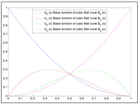
Figure 1. Cubic Ball curve basis functions.

The first advantage of the cubic basis function of Ball curves is that it can be reduced to the quadratic basis function of Bézier curves when combined with its internal control points. Secondly, the basis function of Ball curves demonstrates better computational performance than Bézier curves when represented in a generalized form [15]. As a result, the Said–Ball curve is slightly more computationally efficient than Bézier curves while maintaining similar shape-preserving properties [15,24,25].

Our study aims to achieve the best approximate solutions for ODEs by enhancing error accuracy through numerical methods. Various algorithms have been developed to solve higher-order ODEs approximately, with a focus on attaining high accuracy [26,27,28,29,30,31,32]. However, challenges such as extensive programming effort, increased human effort, and computational burden can affect the accuracy of these methods.

In the 1960s, Rutishauser introduced a direct method for solving higher-order ODEs without reducing them to systems of first-order ODEs [28], offering an efficient alternative to reduction methods. Earlier, in 1795, Gauss introduced the least squares method (LSM), one of the first direct approaches, which utilizes polynomial or piecewise polynomial functions to approximate solutions to higher-order ODEs and discretize integrals [29]. For solving ODEs, the LSM combined with Bézier curves has been employed as an alternative to integral discretization and has minimized an objective function to determine the Bézier curve’s control points [30]. Additionally, the LSM has been successfully applied to various differential equations in combination with other techniques [4,33,34,35,36,37,38,39,40]. Its simplicity and ability to improve the accuracy of approximate solutions make the LSM advantageous for solving higher-order ODEs [3,25,39,41].

To the best of our knowledge, the use of Said–Ball curves combined with the LSM to improve error accuracy in ODE solutions has not been explored. This research aims to determine the optimal control points of Said–Ball curves using the LSM for improved approximate solutions of ODEs.

Specifically, the objectives are as follows:

i.

To identify the best control points of Said–Ball curves by minimizing the residual error through the sum of the squares of the residual function.

ii.

To achieve better approximate solutions by substituting these optimized control points into Said–Ball curves.

iii.

To significantly improve error accuracy compared to existing methods.

iv.

To establish Said–Ball curve representations with the LSM as a suitable alternative method, contributing to analytical approximations for solving BVPs of ODEs.

The content of this paper is organized as follows: Section 2 provides an overview of Bezier curve representations. Section 3 introduces the representations and properties of Said–Ball curves. Section 4 describes the proposed method, using Said–Ball curves with the LSM to approximate ODE solutions. Section 5 provides a convergence analysis of the method. Numerical examples validating the proposed method are presented in Section 6, followed by the results in Section 7. Finally, Section 8 concludes the study.

2. Bézier Curves

From [30], Bézier curves of degree $m$ can be defined using $\left(m+1\right)$ control points ${\left\{b_j\right\}}_{j=0}^m$ as follows:

$$B\left(x\right)={\sum }_{j=0}^m{b}_j{B}_j^m\left({\displaystyle \frac{x-a}{b-a}}\right), a\le x\le b,$$

(2)

where $b_j$ are the Bézier control points (or Bézier coefficients), and the polynomials of Bézier curves $B_j^m\left(x\right)$ in the interval [a, b] are as follows:

$$B_j^m\left({\displaystyle \frac{x-a}{b-a}}\right)=\left({\displaystyle \genfrac{}{}{0pt}{}{m}{j}}\right){\left({\displaystyle \frac{x-a}{b-a}}\right)}^j{\left({\displaystyle \frac{b-x}{b-a}}\right)}^{m-j}$$

In particular,

$$B\left(x\right)=\sum _{j=0}^m{b}_j{B}_j^m\left(x\right), 0\le x\le 1,$$

(3)

where

$$B_j^m\left(x\right)=\left({\displaystyle \genfrac{}{}{0pt}{}{m}{j}}\right)x^j{\left(1-x\right)}^{m-j}.$$

The function $B\left(x\right)$ is a parametric Bézier curve if it is a polynomial in the form of a vector-valued function. Moreover, its control polygon contains of the line segments $b_j-b_{j+1},$ where $j=0, 1, 2, \dots , m-1$. If $B\left(x\right)$ is a scalar-valued function, then the function $y=B\left(x\right)$ is known as an explicit Bézier curve, represented by $(x, B\left(x\right))$.

3. Said–Ball Curves

From [15,22,42,43], Said–Ball curves of degree $m$ are defined as follows:

$$S\left(x\right)={\sum }_{j=0}^m{S}_j^m\left(x\right)v_{j },$$

(4)

where ${\left\{v_j\right\}}_{j=0}^m$ are the $m+1$ control points,

$$S_j^m\left(x\right)=\left\{\begin{array}{c}\left(\begin{array}{c}{\displaystyle \frac{m-1}{2}}+j\\ j\end{array}\right)x^j{\left(1-x\right)}^{{\displaystyle \frac{m+1}{2}}},\hspace{1em}\hspace{1em}\hspace{1em}for 0\le j\le {\displaystyle \frac{m-1}{2}}\\ \left(\begin{array}{c}{\displaystyle \frac{m-1}{2}}+m-j\\ m-j\end{array}\right)x^{{\displaystyle \frac{m+1}{2}}}{\left(1-x\right)}^{m-j},\hspace{1em}\hspace{1em}\hspace{1em}for {\displaystyle \frac{m+1}{2}}\le j\le m \end{array}\right.$$

(5)

when $m$ is odd, and

$$S_j^m\left(x\right)=\left\{\begin{array}{c}\left(\begin{array}{c}{\displaystyle \frac{m}{2}}+j\\ j\end{array}\right)x^j{(1-x)}^{{\displaystyle \frac{m}{2}}+1}, for 0\le j\le {\displaystyle \frac{m}{2}}-1 \\ \left(\begin{array}{c}m\\ {\displaystyle \frac{m}{2}}\end{array}\right)x^{{\displaystyle \frac{m}{2}}}{\left(1-x\right)}^{{\displaystyle \frac{m}{2}}}, for j={\displaystyle \frac{m}{2}}\\ \left(\begin{array}{c}{\displaystyle \frac{m}{2}}+m-j\\ m-j\end{array}\right)x^{{\displaystyle \frac{m}{2}}+1}{\left(1-x\right)}^{m-j}, for {\displaystyle \frac{m}{2}}+1\le j\le m\end{array}\right.$$

(6)

when m is even.

Properties:

$$\mathbf{i}. S_j^m\left(x\right)\ge 0, \mathrm{for} \mathrm{all} j=0,1,2,\dots ,m.$$

(7)

$$\mathbf{ii}. {\sum }_{j=0}^m{S}_j^m\left(x\right)=1.$$

(8)

The properties in Equations (7) and (8) demonstrate the convex combination of the control points. Hence, the Said–Ball curve’s control polygon lies within the convex hull [22].

The basis functions of Said–Ball curves of degrees two, three, four, and five are presented in Equations (8a), (8b), (8c), and (8d), respectively:

$$\begin{array}{l}{S}_1\left(x\right)=S_0^2\left(x\right)={(1-x)}^2,\hspace{1em}{S}_2\left(x\right)=S_1^2\left(x\right)=2x\left(1-x\right),\\ \hspace{1em}\hspace{1em}\hspace{1em}{S}_3\left(x\right)=S_2^2\left(x\right)=x^2;\end{array}$$

(8a)

$$\begin{array}{l}{S}_1\left(x\right)=S_0^3\left(x\right)={(1-x)}^2,\hspace{1em}{S}_2\left(x\right)=S_1^3\left(x\right)=2x{(1-x)}^2,\\ \hspace{1em}\hspace{1em}\hspace{1em}\hspace{1em}\hspace{1em}\hspace{1em}\hspace{1em}\hspace{1em}{S}_3\left(x\right)=S_2^3\left(x\right)=2x^2\left(1-x\right),\hspace{1em}{S}_4\left(x\right)=S_3^3\left(x\right)=x^2;\end{array}$$

(8b)

$$\begin{array}{l}{S}_1\left(x\right)=S_0^4\left(x\right)={(1-x)}^3,\hspace{1em}{S}_2\left(x\right)=S_1^4\left(x\right)=3x{(1-x)}^3,\\ \hspace{1em}\hspace{1em}\hspace{1em}\hspace{1em}\hspace{1em}\hspace{1em}\hspace{1em}\hspace{1em}{S}_3\left(x\right)=S_2^4\left(x\right)=6x^2{(1-x)}^2,\\ \hspace{1em}\hspace{1em}\hspace{1em}\hspace{1em}\hspace{1em}\hspace{1em}\hspace{1em}\hspace{1em}{S}_4\left(x\right)=S_3^4\left(x\right)=3x^3\left(1-x\right),\hspace{1em}{S}_5\left(x\right)=S_4^4\left(x\right)=x^3;\end{array}$$

(8c)

$$\begin{array}{l}{S}_1\left(x\right)=S_0^5\left(x\right)={(1-x)}^3,\hspace{1em}{S}_2\left(x\right)=S_1^5\left(x\right)=3x{(1-x)}^3,\\ \hspace{1em}\hspace{1em}\hspace{1em}\hspace{1em}\hspace{1em}\hspace{1em}\hspace{1em}\hspace{1em}{S}_3\left(x\right)=S_2^5\left(x\right)=6x^2{(1-x)}^3,\\ \hspace{1em}\hspace{1em}\hspace{1em}\hspace{1em}\hspace{1em}\hspace{1em}\hspace{1em}\hspace{1em}{S}_4\left(x\right)=S_3^5\left(x\right)=3x^3{(1-x)}^2,\\ \hspace{1em}\hspace{1em}\hspace{1em}\hspace{1em}\hspace{1em}\hspace{1em}\hspace{1em}\hspace{1em}{S}_5\left(x\right)=S_4^5\left(x\right)=3x^3\left(1-x\right),\hspace{1em}{S}_6\left(x\right)=S_5^5\left(x\right)=x^3.\end{array}$$

(8d)

Figure 2, Figure 3, Figure 4 and Figure 5 below each show the graphs of the basis functions of Said–Ball curves of degrees two, three, four, and five, respectively.

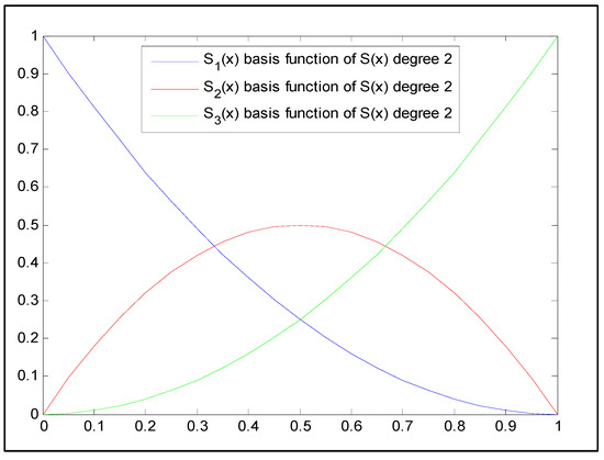
Figure 2. Said–Ball curve with degree 2 basis functions.

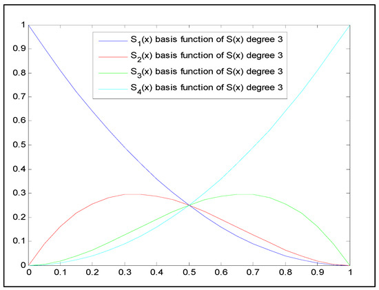
Figure 3. Said–Ball curve with degree 3 basis functions.

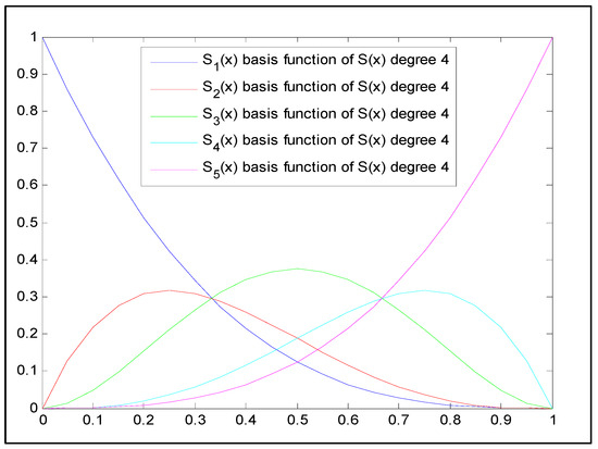
Figure 4. Said–Ball curve with degree 4 basis functions.

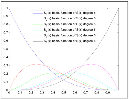
Figure 5. Said–Ball curve with degree 5 basis functions.

4. Least Squares Method for Solving ODEs

4.1. Exploration of Said–Ball Curve’s Control Points Technique

The Said–Ball curves are proposed as a technique based on their control points, as the basis function of Said–Ball curves offers better computational capability than the basis function of Bézier curves.

The strategies involved in the study are as follows:

• Exploring the optimal control points using the LSM.
• Computing the control points by minimizing the residual function through the LSM.

Consider the following ${\left(2n\right)}^{th}$-order ODE:

$$Lg\left(x\right)={\sum }_{i=0}^{2n}{\phi }_i\left(x\right){\displaystyle \frac{d^i}{{dx}^i}}\left[g\left(x\right)\right]=f\left(x\right), 0\le x\le 1,$$

(9)

with initial conditions:

$${\displaystyle \frac{d^i}{{dx}^i}}\left[g\left(0\right)\right]={\eta }_i, i=\mathrm{0,1}, 2, \dots , n-1,$$

(10)

and boundary conditions:

$${\displaystyle \frac{d^i}{{dx}^i}}\left[g\left(0\right)\right]={\eta }_i,{\displaystyle \frac{d^i}{{dx}^i}}\left[g\left(1\right)\right]={\xi }_i,i=0,1,2,\dots ,n-1,$$

(11)

where

$$L={\sum }_{i=0}^{2n}{\phi }_i\left(x\right){\displaystyle \frac{d^i}{{dx}^i}}$$

is the ${\left(2n\right)}^{th}$-order differential operator with the polynomial coefficients ${\phi }_i\left(x\right)$ and $f\left(x\right)$ is a polynomial function.

The residual error is measured by minimizing the residual function as follows:

$$R\left(x\right)=Lg\left(x\right)-f\left(x\right),$$

(12)

The minimization of the residual function is achieved by summing the squares of the residual values at the control points. This summation becomes zero when the residual error at all control points is zero, indicating that the approximate solution matches the exact solution.

To address this, a new algorithm is proposed to obtain the approximate solution of Equation (9) while satisfying the initial conditions in Equation (10) and the boundary conditions in Equation (11). The algorithm is described as follows:

Step 1: Represent the approximate solution using Said–Ball curves of degree $m$, where $m\ge$ the order of the differential equation, i.e.,

$$S\left(x\right)={\sum }_{j=0}^m{S}_j^m\left(x\right)v_j, 0\le x\le 1,$$

(13)

where the $\left(m+1\right)$ control points ${\left\{v_j\right\}}_{j=0}^m=v_0,v_1,v_2,\dots ,v_m$ need to be calculated.

Step 2: Compute the residual function $R_S\left(x\right)=Lg\left(x\right)-f\left(x\right)$ by substituting $S\left(x\right)$ into Equation (9) while incorporating the initial and boundary conditions given in Equations (10) and (11). The residual function can be expressed as a polynomial:

$$R_S\left(x\right)=\sum _{j=0}^k{ c}_{Sj}{ S}_j^m\left(x\right),$$

which is represented using Said–Ball curves of degree $\le k$, where

$$k=\underset{j}{\max }\left\{m-j+\mathrm{deg}\left({\phi }_j\right),\mathrm{deg}\left(f\left(x\right)\right)\right\}.$$

Here, $c_{Sj}$ are the control points of $R_S\left(x\right)$, expressed as linear functions of the unknowns $v_j$, with $j=0, 1, 2, 3,\dots , k$.

Step 3: Develop the objective function for Said–Ball curves:

$$F_S=\sum _{j=0}^k{c}_{Sj}^2{v}_j.$$

Step 4: Solve for the control points $v_j$ by addressing the constrained optimization problem:

$$\min F_S =\sum _{j=0}^k{c}_{Sj}^2{v}_j,$$

subject to the following conditions

$${\displaystyle \frac{d^i}{{dx}^i}}\left[g\left(0\right)\right]={\eta }_j \mathrm{a}\mathrm{n}\mathrm{d} {\displaystyle \frac{d^i}{{dx}^i}}\left[g\left(1\right)\right]={\xi }_j,j=0,1,2,\dots ,m-1.$$

To solve this constrained optimization problem, any suitable method can be applied, such as the Lagrange Multiplier Method.

Step 5: Substitute the calculated control points $v_j$ back into Equation (13) to obtain the approximate solution of Equation (9).

4.2. Degree-Raising Scheme

In Section 4.1, the control points-based method using the LSM provides an approximate solution to the ODEs. By substituting the values of Said–Ball curve control points $v_j$ back into the objective function $F_s$, the Euclidean norm of the Said–Ball curve’s control points can be computed. This enables determining an upper bound for the residual function $R_s\left(x\right)$ based on the values of $c_j$, expressed as

$$\left|R_s\left(x\right)\right|\le {max}_j\left\{\left|c_j\right|\right\},\hspace{1em}\hspace{1em}0\le x\le 1.$$

(14)

If the obtained error values are not sufficiently small, the approximate solution does not meet the expected accuracy level. To address this, the degree of the Said–Ball curve, which serves as the approximate solution, can be increased. By repeating the process outlined in Section 4.1 with the updated curve degree, an improved solution can be achieved, meeting the desired level of accuracy and reducing the error.

4.3. Performance Comparison

The proposed method was implemented in MATLAB-R2020a and applied to solve BVPs for second-order and fourth-order ODEs. The error metrics, including error accuracy, maximum absolute error, maximum relative error, and maximum percent relative error of the exact and approximate solutions based on Said–Ball curves, were compared with existing methods such as the Bézier curve method [30], the direct inverse method, the steepest descent method, and FMARI [36].

The formulas for the three types of errors are as follows:

$$\mathbf{A}\mathbf{b}\mathbf{s}\mathbf{o}\mathbf{l}\mathbf{u}\mathbf{t}\mathbf{e} \mathbf{E}\mathbf{r}\mathbf{r}\mathbf{o}\mathbf{r} = \left|\mathrm{E}\mathrm{x}\mathrm{a}\mathrm{c}\mathrm{t} \mathrm{V}\mathrm{a}\mathrm{l}\mathrm{u}\mathrm{e}-\mathrm{A}\mathrm{p}\mathrm{p}\mathrm{r}\mathrm{o}\mathrm{x}\mathrm{i}\mathrm{m}\mathrm{a}\mathrm{t}\mathrm{e} \mathrm{V}\mathrm{a}\mathrm{l}\mathrm{u}\mathrm{e}\right|,$$

$$\mathbf{R}\mathbf{e}\mathbf{l}\mathbf{a}\mathbf{t}\mathbf{i}\mathbf{v}\mathbf{e} \mathbf{E}\mathbf{r}\mathbf{r}\mathbf{o}\mathbf{r}=\left|{\displaystyle \frac{\mathrm{E}\mathrm{x}\mathrm{a}\mathrm{c}\mathrm{t} \mathrm{V}\mathrm{a}\mathrm{l}\mathrm{u}\mathrm{e}-\mathrm{A}\mathrm{p}\mathrm{p}\mathrm{r}\mathrm{o}\mathrm{x}\mathrm{i}\mathrm{m}\mathrm{a}\mathrm{t}\mathrm{e} \mathrm{V}\mathrm{a}\mathrm{l}\mathrm{u}\mathrm{e}}{Exact Value}}\right|,$$

$$\mathbf{P}\mathbf{e}\mathbf{r}\mathbf{c}\mathbf{e}\mathbf{n}\mathbf{t} \mathbf{R}\mathbf{e}\mathbf{l}\mathbf{a}\mathbf{t}\mathbf{i}\mathbf{v}\mathbf{e} \mathbf{E}\mathbf{r}\mathbf{r}\mathbf{o}\mathbf{r}=\left|{\displaystyle \frac{\mathrm{E}\mathrm{x}\mathrm{a}\mathrm{c}\mathrm{t} \mathrm{V}\mathrm{a}\mathrm{l}\mathrm{u}\mathrm{e}-\mathrm{A}\mathrm{p}\mathrm{p}\mathrm{r}\mathrm{o}\mathrm{x}\mathrm{i}\mathrm{m}\mathrm{a}\mathrm{t}\mathrm{e} \mathrm{V}\mathrm{a}\mathrm{l}\mathrm{u}\mathrm{e}}{\mathrm{E}\mathrm{x}\mathrm{a}\mathrm{c}\mathrm{t} \mathrm{V}\mathrm{a}\mathrm{l}\mathrm{u}\mathrm{e}}}\right|\times 100\%.$$

The method with the smallest error across all metrics is considered the best-performing approach.

5. Convergence Analysis

A convergence analysis of the proposed technique is conducted based on the Said–Ball curve’s control points. The analysis focuses on a two-point BVP with a unique $C^2$ smooth solution, ensuring the method’s robustness in producing solutions that converge to the exact values under appropriate conditions.

Consider the following BVP:

$$Lg\left(x\right)={\phi }_2\left(x\right)g^{″}\left(x\right)+{\phi }_1\left(x\right)g^{\prime }\left(x\right)+{\phi }_0\left(x\right)g\left(x\right)=f\left(x\right),\hspace{1em}\hspace{1em}\hspace{1em}0\le x\le 1,$$

(15)

with $g\left(0\right)=c,g\left(1\right)=d,$ where ${\phi }_0, {\phi }_1, {\phi }_2$, and $f$ are polynomials in terms of $x$.

By averaging the control points of Said–Ball curves, the square of the $L_2$ norm polynomial can be approximated over the interval $0\le x\le 1$ based on the control points of the Said–Ball curve.

Lemma 1.

If the Said–Ball curves represented in the form of a polynomial are

$$S\left(x\right)=\sum _{j=0}^m{v}_{j,m}{S}_j^m\left(x\right),$$

then

$${\displaystyle \frac{1}{m+1}}{\sum }_{j=0}^m{v}_{j,m}^2\ge {\displaystyle \frac{1}{m+2}}{\sum }_{j=0}^{m+1}{v}_{j,m+1}^2\ge {\displaystyle \frac{1}{m+3}}{\sum }_{j=0}^{m+2}{v}_{j,m+2}^2\ge \cdots \ge {\displaystyle \frac{1}{m+n+1}}{\sum }_{j=0}^{m+n}{v}_{j,m+n}^2\to {\int }_0^1{S}^2\left(x\right)dx, n\to +\mathrm{\infty },$$

where $v_{j, m+k}$ are the control points of Said–Ball curves after increasing the degree to $m+k$.

Proof. 

By using the degree-raising rule

$$v_{j,m+1}={\displaystyle \frac{j}{m+1}}{v}_{j-1,m}+{\displaystyle \frac{m+1-j}{m+1}}{v}_{j,m},$$

hence,

$$\begin{array}{l}\hspace{1em}{\displaystyle \frac{1}{m+2}}{\sum }_{j=0}^{m+1}{v}_{j,m+1}^2\\ \hspace{1em}\hspace{1em}={\displaystyle \frac{1}{m+2}}{\displaystyle \sum _{j=0}^{m+1}}\left[{\left({\displaystyle \frac{j}{m+1}}\right)}^2{v}_{j-1,m}^2+{\left({\displaystyle \frac{m+1-j}{m+1}}\right)}^2{v}_{j,m}^2+2{\displaystyle \frac{j(m+1-j)}{{(m+1)}^2}}{v}_{j-1,m} v_{j,m}\right]\\ \le {\displaystyle \frac{1}{m+2}}\left[{\displaystyle \sum _{j=1}^{m+1}}{\left({\displaystyle \frac{j}{m+1}}\right)}^2{v}_{j-1,m}^2+{\displaystyle \sum _{j=0}^m}{\left({\displaystyle \frac{m+1-j}{m+1}}\right)}^2{v}_{j,m}^2+{\displaystyle \sum _{j=1}^m}{\displaystyle \frac{j\left(m+1-j\right)}{{\left(m+1\right)}^2}}\left(v_{j-1,m}+v_{j,m}\right)\right]\\ \hspace{1em}\hspace{1em}={\displaystyle \frac{1}{m+1}}{\displaystyle \sum _{j=0}^m}{v}_{j,m}^2.\end{array}$$

This demonstrates that the sequence

$$\left\{{\displaystyle \frac{1}{m+n+1}}{\sum }_{j=0}^{m+n}{v}_{j,m+n}^2\right\}.$$

is monotonically decreasing and converges as $n\to +\mathrm{\infty }$, with the lower bound being zero. It remains to prove that ${\int }_0^1{S}^2\left(x\right)dx$ is equal to the limit of the above sequence.

Using the definition of the definite integration, we have

$${\int }_0^1{S}^2\left(x\right)dx=\underset{n\to +\mathrm{\infty }}{\mathit{lim}}\left({\displaystyle \frac{1}{m+n+1}}{\sum }_{j=0}^{m+n}{S}^2\left({\displaystyle \frac{j}{m+n}}\right)\right).$$

From the convergence property of the Said–Ball curves’ degree raising, there exists an arbitrarily small positive number ${\epsilon }_j$ $(j=0,1,2,3,...,m+n)$ such that

$$S\left({\displaystyle \frac{j}{m+n}}\right)=v_{j,m+n}+{\epsilon }_j, j=0,1,2,3,...,m+n,$$

with

$$\underset{n\to +\mathrm{\infty }}{\mathit{lim}}{\mathit{max}}_j\left|{\epsilon }_j\right|=0.$$

Hence,

$${\displaystyle \frac{1}{m+n+1}}{\sum }_{j=0}^{m+n}{S}^2\left({\displaystyle \frac{j}{m+n}}\right)={\displaystyle \frac{1}{m+n+1}}{\sum }_{j=0}^{m+n}\left(v_{j,n+m}^2+2v_{j,m+n}{\epsilon }_j+{\epsilon }_j^2\right).$$

Let

$${\epsilon }_{m,n}={max}_j{\left\{\left|{\epsilon }_j\right|\right\}}_{j=0}^{m+n}.$$

Now, we estimate the last two terms in the right-hand side of the equation as follows:

$$\left|{\displaystyle \frac{1}{m+n+1}}{\sum }_{j=0}^{m+n}\left({\epsilon }_j^2\right)\right|\le {\epsilon }_{m,n}^2$$

and

$$\begin{array}{c}\left|{\displaystyle \frac{1}{m+n+1}}{\displaystyle \sum _{j=0}^{m+n}}\left(v_{j,m+n}{\epsilon }_j\right)\right|\le {\displaystyle \frac{1}{m+n+1}}{\epsilon }_{m,n}{\displaystyle \sum _{j=0}^{m+n}}\left|v_{j,m+n}\right|\hfill \\ \hspace{1em}\hspace{1em}\hspace{1em}\hspace{1em}\hspace{1em}\hspace{1em}\hspace{1em}\hspace{1em}\hspace{1em}\hspace{1em}\hspace{1em}\hspace{1em} \le {\displaystyle \frac{1}{m+n+1}} \left[{\epsilon }_{m,n}{\displaystyle \sum _{j=0}^{m+n}}\right({\displaystyle \frac{j}{m+n}}\left|v_{j-1,m+n-1}\right|\hfill \\ \hspace{1em}\hspace{1em}\hspace{1em}\hspace{1em}\hspace{1em}\hspace{1em}\hspace{1em}\hspace{1em}\hspace{1em}\hspace{1em}\hspace{1em}\hspace{1em}\hspace{1em}\hspace{1em}\hspace{1em}\hspace{1em}\hspace{1em}\hspace{1em}\hspace{1em}\hspace{1em}+{\displaystyle \frac{m+n-j}{m+n}}\left|v_{j,m+n-1}\right|\left)\right]\hfill \\ \hspace{1em}\hspace{1em}\hspace{1em}\hspace{1em}\hspace{1em}\hspace{1em}\hspace{1em}\hspace{1em}\hspace{1em}\le {\displaystyle \frac{1}{m+n}}{\epsilon }_{m,n}{\sum }_{j=0}^{m+n-1}\left|v_{j,m+n-1}\right|\le \cdots \le {\displaystyle \frac{1}{m+1}}{\epsilon }_{m,n}{\sum }_{j=0}^m\left|v_{j,m}\right|.\hfill \end{array}$$

Hence,

$$\underset{n\to +\mathrm{\infty }}{\mathit{lim}}\left[{\displaystyle \frac{1}{m+n+1}}{\sum }_{j=0}^{m+n}\left(2v_{j,m+n}{\epsilon }_j+{\epsilon }_j^2\right)\right]=0.$$

Thus,

$$\underset{n\to +\mathrm{\infty }}{lim}\left[{\displaystyle \frac{1}{m+n+1}}{\sum }_{j=0}^{m+n}{S}^2\left({\displaystyle \frac{j}{m+n}}\right)\right]=\underset{n\to +\mathrm{\infty }}{lim}\left[{\displaystyle \frac{1}{m+n+1}}{\sum }_{j=0}^{m+n}\left(v_{j,n+m}^2\right)\right].$$

□

Theorem 1.

Let $g\left(x\right)$ be the $C^2$-continuous and unique solution of the two-point BVP (15). The approximate solution $g_n\left(x\right)$ constructed using the control points of Said–Ball curves, converges to the exact solution g(x) as the degree of the approximate solution tends to infinity.

Proof. The proof is divided into several steps:

• Step 1.

Given an arbitrarily small number $\epsilon >0$, the Weierstrass theorem [25,37,38] guarantees the existence of a polynomial $H_K$ of degree $K$ such that

$${‖{\displaystyle \frac{d^j{H}_K\left(x\right)}{{dx}^j}}-{\displaystyle \frac{d^{j}g\left(x\right)}{{dx}^j}}‖}_{\mathrm{\infty }}<{\displaystyle \frac{\epsilon }{2}}, j=0,1,2,$$

where ${‖.‖}_{\mathrm{\infty }}$ denotes the $L_{\mathrm{\infty }}$-norm over $0\le x\le 1$.

However, $H_K\left(x\right)$ may not generally satisfy the given boundary conditions. By applying a small perturbation in the form of a linear polynomial $ax+b$, we construct another polynomial $G_K\left(x\right)=H_K\left(x\right)+ax+b$ such that $G_K\left(x\right)$ satisfies the boundary conditions $G_K\left(0\right)=c$ and $G_K\left(1\right)=d,$ and

$${‖{\displaystyle \frac{d^j{G}_K\left(x\right)}{{dx}^j}}-{\displaystyle \frac{d^{j}g\left(x\right)}{{dx}^j}}‖}_{\mathrm{\infty }}<\epsilon ,j=0,1,2.$$

Hence, the residual function can be estimated as follows:

$$\begin{array}{l}{‖L{G}_K\left(x\right)-f\left(x\right)‖}_{\mathrm{\infty }}={‖L\left(G_K\left(x\right)-g\left(x\right)\right)‖}_{\mathrm{\infty }}\\ \hspace{1em}\hspace{1em}\hspace{1em}\hspace{1em}\hspace{1em}\hspace{1em}\hspace{1em}\le {‖{\phi }_2\left(x\right)‖}_{\mathrm{\infty }}{‖G_K^{″}-g^{″}‖}_{\mathrm{\infty }}+{‖{\phi }_1\left(x\right)‖}_{\mathrm{\infty }}{‖G_K^{\prime }-g^{\prime }‖}_{\mathrm{\infty }}+{‖{\phi }_0\left(x\right)‖}_{\mathrm{\infty }}{‖G_K-g‖}_{\mathrm{\infty }}\\ \hspace{1em}\hspace{1em}\hspace{1em}\hspace{1em}\hspace{1em}\hspace{1em}\hspace{1em}\le \left({‖{\phi }_2\left(x\right)‖}_{\mathrm{\infty }}+{‖{\phi }_1\left(x\right)‖}_{\mathrm{\infty }}+{‖{\phi }_0\left(x\right)‖}_{\mathrm{\infty }}\right)\epsilon \end{array}$$

where ${‖{\phi }_2\left(x\right)‖}_{\mathrm{\infty }}+{‖{\phi }_1\left(x\right)‖}_{\mathrm{\infty }}+{‖{\phi }_0\left(x\right)‖}_{\mathrm{\infty }}$ is a constant.

• Step 2.

In this step, we represent the residual in the form of the Said–Ball curve as follows:

$$R(G_K):=L\left(G_K\right)-f\left(x\right)=\sum _{j=0}^m{v}_{j,m}{S}_j^m\left(x\right)$$

From Lemma 1, there exists an integer $N(\ge M)$ such that if $n>N$, then

$$\left|{\displaystyle \frac{\sum _{j=0}^m{v}_{j,m}^2}{m+1}}-\underset{0}{\overset{1}{\int }}{\left(R\left(G_K\right)\right)}^{2}dx\right|<\epsilon$$

$$⟹{\displaystyle \frac{\sum _{j=0}^m{v}_{j,m}^2}{m+1}}<\epsilon +\underset{0}{\overset{1}{\int }}{\left(R\right(G_K)}^{2}dx\le \epsilon +{\left[\left({‖{\phi }_2\left(x\right)‖}_{\mathrm{\infty }}+{‖{\phi }_1\left(x\right)‖}_{\mathrm{\infty }}+{‖{\phi }_0\left(x\right)‖}_{\mathrm{\infty }}\right)\epsilon \right]}^2.$$

• Step 3.

Now, suppose that $g_n\left(x\right)$ is the approximate solution of (15) with degree $n\ge N$ constructed using the control points of Said–Ball curves. Let

$$R(g_n\left(x\right))=L\left(g_n\left(x\right)\right)-f\left(x\right)=\sum _{j=0}^l{c}_{j,l}{S}_j^l\left(x\right)$$

with degree $l\ge n\ge N$.

Further, we estimate the Sobolev norm of the difference in the exact solution $g\left(x\right)$ and the approximate solution $g_n\left(x\right)$ as follows:

$${‖g_n\left(x\right)-g\left(x\right)‖}_{H^2\left[0,1\right]}≔\underset{0}{\overset{1}{\int }}\sum _{i=0}^2{\left|{\displaystyle \frac{d^i{g}_n\left(x\right)}{{dx}^i}}-{\displaystyle \frac{d^{i}g\left(x\right)}{{dx}^i}}\right|}^{2}dx$$

$$\le T\left(\left|g_n\left(0\right)-g\left(0\right)\right|+\left|g_n\left(1\right)-g\left(1\right)\right|+{‖R\left(g_n\left(x\right)-g\left(x\right)\right)‖}_2\right)=T\underset{0}{\overset{1}{\int }}{\left(\sum _{j=0}^l{c}_{j,l}{S}_j^l\left(x\right)\right)}^{2}dx\le {\displaystyle \frac{T}{l+1}}\sum _{j=0}^l{c}_{j,l}^2.$$

Here, $T$ is a constant. Since the average of the squared residuals at the control points of the Said–Ball curves is minimized using the control points-based method, the average value of the approximate solution $g_n\left(x\right)$ is smaller than $G_K\left(x\right)$.

Thus,

$$\begin{array}{l}{‖g_n\left(x\right)-g\left(x\right)‖}_{H^2[0,1]}\le {\displaystyle \frac{T}{l+1}}\sum _{j=0}^l{c}_{j,l}^2\le {\displaystyle \frac{T}{l+1}}\sum _{j=0}^l{v}_{j,l}^2\le {\displaystyle \frac{T}{m+1}}\sum _{j=0}^m{v}_{j,l}^2\\ \hspace{1em}\hspace{1em}\hspace{1em}\hspace{1em}\hspace{1em}\hspace{1em}\hspace{1em}\le T\left(\epsilon {+\left(\left({‖{\phi }_2\left(x\right)‖}_{\mathrm{\infty }}+{‖{\phi }_1\left(x\right)‖}_{\mathrm{\infty }}+{‖{\phi }_0\left(x\right)‖}_{\mathrm{\infty }}\right)\epsilon \right)}^2\right).\end{array}$$

Hence, the approximate solution converges to the exact solution as the degree of the approximate solution approaches infinity. □

6. Numerical Examples

Four numerical examples from related works were considered to demonstrate the proposed method. The basis function of the Said–Ball curve was used to approximate the solution of BVPs involving second-order and fourth-order ODEs, as well as second-order non-homogeneous ODEs, utilizing the LSM. The results and accuracy, in terms of error, were compared with those from existing studies.

The maximum absolute error, relative error, and percent relative error between the exact and approximate solutions based on Said–Ball curves were compared with those obtained using the Bézier curve method [30], the direct inverse method, the steepest descent method, and FMARI [36].

6.1. Example 1: [30]

To illustrate the method, a very simple example is considered as the first case.

Consider

$$\begin{gathered} y^{″}\left(x\right)-6x=0, \\ y\left(0\right)=0,\hspace{1em}y\left(1\right)=1. \end{gathered}$$

The exact solution of the above BVP is $y_e\left(x\right)=x^3$.

Suppose that a degree-2 Said–Ball curve is used to represent the approximate solution.

$$\begin{array}{c}\hspace{1em}\hspace{1em}\hspace{1em}\hspace{1em}{y}_a\left(x\right)=S_a\left(x\right)={\displaystyle \sum _{j=0}^2}{S}_j^m\left(x\right)v_j=v_0{S}_0^2\left(x\right)+v_1{S}_1^2\left(x\right)+v_2{S}_2^2\left(x\right)\hfill \\ =v_0{\left(1-x\right)}^2+v_{1}2x\left(1-x\right)+v_2{x}^2.\hfill \end{array}$$

(16)

The residual function is obtained by substituting $y_a\left(x\right)=S_a\left(x\right)$ into the given ODE:

$$\begin{array}{l}{R}_S\left(x\right)=2v_0-4v_1+2v_2-6\\ \hspace{1em}\hspace{1em}\hspace{1em}\hspace{1em}\hspace{1em}\hspace{1em}\hspace{1em}=\left(2v_0-4v_1+2v_2\right)S_0^2\left(x\right)+\left(2v_0-4v_1+2v_2-6x\right)S_1^2\left(x\right).\end{array}$$

The objective function is developed as follows:

$$F_S(v_0,v_1,v_2)={\left(2v_0-4v_1+2v_2\right)}^2+{\left(2v_0-4v_1+2v_2-6\right)}^2.$$

The values of $v_0, v_1,{\mathrm{a}\mathrm{n}\mathrm{d} v}_2$ were determined by applying the proposed technique with the boundary conditions $y\left(0\right)=0 \mathrm{a}\mathrm{n}\mathrm{d} y\left(1\right)=1$, resulting in $v_0=0, v_1=0,$ and $v_2=1$.

These control points values were substituted into Equation (16); yielding the approximate solution as follows:

$$y_a\left(x\right)=S_a\left(x\right)=x^2.$$

(17)

The exact solution and the approximate solution using a degree-2 Said–Ball curve are presented graphically in Figure 6.

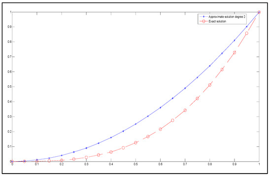
Figure 6. The exact solution $y_e\left(x\right)$ (represented by circles with dashed lines) and the approximate solution $y_a\left(x\right)$ (represented by stars with dashed lines) for degree 2.

Next, Example 1 is reconsidered by increasing the degree of the Said–Ball curve to 3 to enhance error accuracy.

$$\begin{gathered} y_a\left(x\right)=S_a\left(x\right)={\sum }_{j=0}^3{S}_j^m\left(x\right)v_j=v_0{S}_0^3\left(x\right)+v_1{S}_1^3\left(x\right)+v_2{S}_2^3\left(x\right)+v_3{S}_3^3\left(x\right). \\ =v_0{\left(1-x\right)}^2+2v_{1}x{\left(1-x\right)}^2+2v_2{x}^2\left(1-x\right)+v_3{x}^2. \end{gathered}$$

(18)

The control points values of the Said–Ball curve in Table 1 were calculated by applying the proposed method with the boundary conditions $y\left(0\right)=0 \mathrm{a}\mathrm{n}\mathrm{d} y\left(1\right)=1$.

Table 1. Control points values of the Said–Ball curve for Example 1.

Control Points	Values
$v_0$	0
$v_1$	0
$v_2$	−0.5
$v_3$	1

Thus, the approximate solution was obtained by substituting the above control points values into Equation (18).

$$\begin{gathered} y_a\left(x\right)=S_a\left(x\right)=2(-0.5)x^2\left(1-x\right)+\left(1\right)x^2 \\ \Rightarrow y_a\left(x\right)=S_a\left(x\right)=x^3. \end{gathered}$$

(19)

The exact solution and the approximate solution using a degree-3 Said–Ball curve are presented graphically in Figure 7.

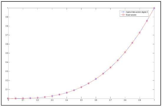
Figure 7. The exact solution $y_e\left(x\right)$ (represented by circles with dashed lines) and the approximate solution $y_a\left(x\right)$ (represented by stars with dashed lines) for degree 3.

In Example 1, the maximum absolute error of 0.147578 occurs at $x=0.65 \mathrm{within} \mathrm{the} \mathrm{interval} 0\le x\le 1$, between the exact solution and the approximate solution of degree 2. However, when the degree of the Said–Ball curve is increased to 3, the approximate solution becomes equivalent to the exact solution.

6.2. Example 2: [30]

$$\begin{gathered} {\left(\left(x^2+1\right)y^{″}\left(x\right)\right)}^{″}=x+1,0<x<1, \\ \mathrm{with} y\left(0\right)=y\left(1\right)=0, y^{\prime }\left(0\right)=y^{\prime }\left(1\right)=0. \end{gathered}$$

The exact solution of the above problem is

$$\begin{array}{l}{y}_e\left(x\right)=[336x\arctan \left(x\right)-36\pi x^2+9{\pi }^2{x}^2+36{\left(\ln 2\right)}^2{x}^2-4\pi x^3+{\pi }^2{x}^3+4{\left(\ln 2\right)}^2{x}^3-44\pi x+168\ln 2x\\ \hspace{1em}\hspace{1em}\hspace{1em}\hspace{1em}\hspace{1em}\hspace{1em}\hspace{1em}-168\ln 2\arctan \left(x\right)+44\pi \arctan \left(x\right)-168\ln \left(1+x^2\right)+44\ln 2\ln \left(1+x^2\right)+42\pi \ln \left(1+x^2\right)\\ \hspace{1em}\hspace{1em}\hspace{1em}\hspace{1em}\hspace{1em}\hspace{1em}\hspace{1em}-84\pi x\arctan \left(x\right)-88\ln 2x\arctan \left(x\right)+22\pi x\ln \left(1+x^2\right)-84\ln 2x\ln \left(1+x^2\right)]\\ \hspace{1em}\hspace{1em}\hspace{1em}\hspace{1em}\hspace{1em}\hspace{1em}\hspace{1em} /36\left(4{\left(\ln 2\right)}^2+{\pi }^2-4\pi \right).\end{array}$$

Firstly, Bézier curves of degrees 5 and 8 are demonstrated as existing methods. For the approximate solution, a Bézier curve of degree 5 is assumed.

$$y_a\left(x\right)=\mathrm{B}\left(x\right)=\sum _{j=0}^5{b}_j B_j^m\left(x\right)$$

$$\begin{array}{c}=b_0{B}_0^5\left(x\right)+b_1{B}_1^5\left(x\right)+b_2{B}_2^5\left(x\right)+b_3{B}_3^5\left(x\right)+b_4{B}_4^5\left(x\right)+b_5{B}_5^5\left(x\right)\hfill \\ =b_0{\left(1-x\right)}^5+5b_1 x{\left(1-x\right)}^4+10b_2{x}^2{\left(1-x\right)}^3+10b_3{x}^3{\left(1-x\right)}^2\hfill \\ +5b_4{x}^4\left(1-x\right)+b_5{x}^5.\end{array}$$

(20)

The control points values of the Bézier curve method in Table 2 were calculated with the boundary conditions $y\left(0\right)=y\left(1\right)=0 \mathrm{a}\mathrm{n}\mathrm{d} y^{\prime }\left(0\right)=y^{\prime }\left(1\right)=0.$

Table 2. Control points values of the Bézier curve of degree 5.

Control Points	Values
$b_0$	0
$b_1$	0
$b_2$	0.0043
$b_3$	0.0033
$b_4$	0
$b_5$	0

Equation (21) is an approximate solution of degree 5, obtained by substituting the control points into Equation (20):

$$y_a\left(x\right)=B\left(x\right)=0.043x^2{\left(1-x\right)}^3+0.033x^3{\left(1-x\right)}^2.$$

(21)

Let the approximate solution be the Bézier curve of degree 8:

$$\begin{array}{ll}{y}_a\left(x\right)& =\mathrm{B}\left(x\right)={\displaystyle \sum _{j=0}^8}{b}_j B_j^m\left(x\right)\\ & =b_0{B}_0^8\left(x\right)+b_1{B}_1^8\left(x\right)+b_2{B}_2^8\left(x\right)+b_3{B}_3^8\left(x\right)+b_4{B}_4^8\left(x\right)+b_5{B}_5^8\left(x\right)\\ & \hspace{1em}\hspace{1em}\hspace{1em}\hspace{1em}\hspace{1em}\hspace{1em}\hspace{1em}+b_6{B}_6^8\left(x\right)+b_7{B}_7^8\left(x\right)+b_8{B}_8^8\left(x\right),\\ & =b_0{\left(1-x\right)}^8+8b_{1}x{\left(1-x\right)}^7+28b_2{x}^2{\left(1-x\right)}^6+56b_3{x}^3{\left(1-x\right)}^5\\ & \hspace{1em}\hspace{1em}\hspace{1em}\hspace{1em}\hspace{1em}\hspace{1em}\hspace{1em}+70b_4{x}^4{\left(1-x\right)}^4+56b_5{x}^5{\left(1-x\right)}^3+28b_6{x}^6{\left(1-x\right)}^2\\ & \hspace{1em}\hspace{1em}\hspace{1em}\hspace{1em}\hspace{1em}\hspace{1em}\hspace{1em}+8b_7{x}^7\left(1-x\right)+b_8{x}^8.\end{array}$$

The control points values of the Bézier curve method in Table 3 were calculated with the boundary conditions $y\left(0\right)=y\left(1\right)=0 \mathrm{a}\mathrm{n}\mathrm{d} y^{\prime }\left(0\right)=y^{\prime }\left(1\right)=0.$

Table 3. Control points values of the Bézier curve of degree 8.

Control Points	Values
$b_0$	0
$b_1$	0
$b_2$	0.0018082143
$b_3$	0.0036007143
$b_4$	0.0040078571
$b_5$	0.0030312500
$b_6$	0.0013717857
$b_7$	0
$b_8$	0

Therefore, the approximate solution of degree 8 is found as follows:

$$\begin{array}{ll}{y}_a\left(x\right)=B\left(x\right)=& 0.05063x^2{\left(1-x\right)}^6+0.20164x^3{\left(1-x\right)}^5+0.280549997x^4{\left(1-x\right)}^4\\ & +0.16975x^5{\left(1-x\right)}^3+0.038409999x^6{\left(1-x\right)}^2.\end{array}$$

The exact solution and the approximate solution using degree-5 and -8 Bézier curves are illustrated graphically in Figure 8.

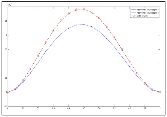
Figure 8. The exact solution $y_e\left(x\right)$ (represented by circles with dashed lines) and the approximate solution $y_a\left(x\right)$ (represented by stars with dashed lines) with Bézier curve of degree 5.

Next, we apply the proposed method to obtain an approximate solution for a BVP involving a fourth-order ODE.

Initially, we assume that the approximate solution is a Said–Ball curve of degree 5.

$$y_a\left(x\right)=S_a\left(x\right)=\sum _{j=0}^5{S}_j^m\left(x\right)v_j=v_0{S}_0^5\left(x\right)+v_1{S}_1^5\left(x\right)+v_2{S}_2^5\left(x\right)+v_3{S}_3^5\left(x\right)+v_4{S}_4^5\left(x\right)+v_5{S}_5^5\left(x\right).$$

$$\begin{array}{c}=v_0{\left(1-x\right)}^3+3v_{1}x{\left(1-x\right)}^3+6v_2{x}^2{\left(1-x\right)}^3+6v_3{x}^3{\left(1-x\right)}^2+3v_4{x}^3\left(1-x\right)+\\ v_5{x}^3.\end{array}$$

(22)

The control points values of the Said–Ball curve in Table 4 were calculated by applying the proposed method with the boundary conditions $y\left(0\right)=y\left(1\right)=0 \mathrm{a}\mathrm{n}\mathrm{d} y^{\prime }\left(0\right)=y^{\prime }\left(1\right)=0$.

Table 4. Control points values of the Said–Ball curve of degree 5 for Example 2.

Control Points	Values
$v_0$	0
$v_1$	0
$v_2$	0.007665
$v_3$	0.005832
$v_4$	0
$v_5$	0

Therefore, the approximate solution is obtained by substituting the values of the control points into Equation (22). Thus, the approximate solution of degree 5 is given by Equation (23):

$$y_a\left(x\right)=S_a\left(x\right)=0.04599x^2{\left(1-x\right)}^3+0.034992x^3{\left(1-x\right)}^2.$$

(23)

The exact solution and the approximate solution using a degree-5 Said–Ball curve are presented graphically in Figure 9.

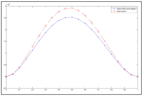
Figure 9. The exact solution $y_e\left(x\right)$ (represented by circles with dashed lines) and the approximate solution $y_a\left(x\right)$ (represented by stars with dashed lines) for degree 5.

Since the approximate solution of degree 5 did not achieve the expected level of accuracy, the degree of the Said–Ball curve is increased. Assume that the approximate solution is the Said–Ball curve of degree 8.

$$\begin{array}{l}{y}_a\left(x\right)=S_a\left(x\right)={\displaystyle \sum _{j=0}^8}{S}_j^m\left(x\right)v_j\\ \hspace{1em}\hspace{1em}\hspace{1em}\hspace{1em}\hspace{1em}\hspace{1em}=v_0{S}_0^8\left(x\right)+v_1{S}_1^8\left(x\right)+v_2{S}_2^8\left(x\right)+v_3{S}_3^8\left(x\right)+v_4{S}_4^8\left(x\right)+v_5{S}_5^8\left(x\right)+v_6{S}_6^8\left(x\right)+v_7{S}_7^8\left(x\right)\\ \hspace{1em}\hspace{1em}\hspace{1em}\hspace{1em}\hspace{1em}\hspace{1em} +v_8{S}_8^8\left(x\right),\\ =v_0{\left(1-x\right)}^5+5v_{1}x{\left(1-x\right)}^5+15v_2{x}^2{\left(1-x\right)}^5+35v_3{x}^3{\left(1-x\right)}^5+70v_4{x}^4{\left(1-x\right)}^4+35v_5{x}^5{\left(1-x\right)}^3\\ \hspace{1em}\hspace{1em}\hspace{1em}\hspace{1em}\hspace{1em}\hspace{1em} +15v_6{x}^5{\left(1-x\right)}^2+5v_7{x}^5\left(1-x\right)+v_8{x}^5.\end{array}$$

Then, the control points $v_0, v_1, v_2, v_3,v_4, v_5, v_6, v_7,$ and $v_8$ are obtained by adopting the proposed method via minimization of the objective function. Their conditions are $y\left(0\right)=y\left(1\right)=0 \mathrm{a}\mathrm{n}\mathrm{d} y^{\prime }\left(0\right)=y^{\prime }\left(1\right)=0$. (see Table 5).

Table 5. Control points values of the Said–Ball curve of degree 8 for Example 2.

Control Points	Values
$v_0$	0
$v_1$	0
$v_2$	0.0033923547
$v_3$	0.0043452293
$v_4$	0.0040366036
$v_5$	0.0037710466
$v_6$	0.0025725930
$v_7$	0
$v_8$	0

Therefore, the approximate solution is obtained by substituting the values of the control points into the above equation. Thus, the approximate solution of degree 8 is given by

$$\begin{array}{c}{y}_a\left(x\right)=0.0508853209x^2{\left(1-x\right)}^5+0.1520830270x^3{\left(1-x\right)}^5+0.2825622496x^4{\left(1-x\right)}^4\\ +0.1319866298x^5{(1-x)}^3+0.0385888955x^5{(1-x)}^2.\end{array}$$

Figure 10 provides a schematic illustration of the exact and approximate solutions of degree 8.

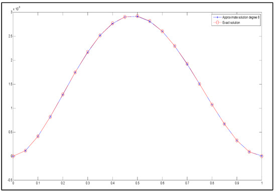
Figure 10. The exact solution $y_e\left(x\right)$ (represented by circles with dashed lines) and the approximate solution $y_a\left(x\right)$ (represented by stars with dashed lines) for degree 8.

6.3. Example 3: A Non-Homogeneous 2nd Order Linear ODE with BVP [36]

$$\begin{array}{ll}& y^{″}+4y=x^2+3e^x,\\ \mathrm{with} & y\left(0\right)=0, y\left(1\right)=2.\end{array}$$

The exact solution of the above BVP is

$$y_e\left(x\right)={\displaystyle \frac{\sin \left(2\right)\left(10x^2+24e^x-19\cos \left(2x\right)-5\right)+\mathrm{s}\mathrm{i}\mathrm{n}\left(2x\right)(-24e+19\cos \left(2\right)+75)}{\left(40\mathrm{s}\mathrm{i}\mathrm{n}\right(2\left)\right)}}.$$

Firstly, assume the Said–Ball curve of degree 3 is the approximate solution to the problem in Example 3.

$$y_a\left(x\right)=S_a\left(x\right)=\sum _{j=0}^3{S}_j^m\left(x\right)v_j=v_0{S}_0^3\left(x\right)+v_1{S}_1^3\left(x\right)+v_2{S}_2^3\left(x\right)+v_3{S}_3^3\left(x\right),$$

$$y_a\left(x\right)=S_a\left(x\right)=v_0{\left(1-x\right)}^2+2v_{1}x{\left(1-x\right)}^2+2v_2{x}^2\left(1-x\right)+v_3{x}^2.$$

(24)

Secondly, the minimization of the objective function with the boundary conditions $y\left(0\right)=0 \mathrm{a}\mathrm{n}\mathrm{d} y\left(1\right)=1$ is performed using the LSM. After that, the constrained optimization problem must be solved in order to obtain the values of the control points for the Said–Ball curve (see Table 6).

Table 6. Control points values of the Said–Ball curve of degree 3 for Example 3.

Control Points	Values
$v_0$	0.0000000002
$v_1$	0.3617523077
$v_2$	0.5333872077
$v_3$	1.9999999952

By substituting the calculated values of the control points of the Said–Ball curve into (24), the approximate solution of the BVP for the 2nd-order non-homogeneous ODE is obtained. Hence, the approximate solution of degree 3 is given in Equation (25).

$$\begin{array}{ll}{y}_a\left(x\right)=S_a\left(x\right)=& 0.0000000002{\left(1-x\right)}^2+0.7235046154x{\left(1-x\right)}^2\\ & +1.0667744154x^2\left(1-x\right)+1.9999999952x^2.\end{array}$$

(25)

Figure 11 presents the approximate and exact solutions graphically.

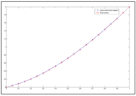
Figure 11. The exact solution $y_e\left(x\right)$ (represented by circles with dashed lines) and the approximate solution $y_a\left(x\right)$ (represented by stars with dashed lines) for degree 3.

Hence, the error accuracy is not at an acceptable level with the degree 3 Said–Ball curve. Now, by increasing the degree of the Said–Ball curve to degree 4, assume the approximate solution of the BVP for the 2nd-order non-homogeneous ODE in the same Example 3.

$$\begin{array}{ll}{y}_a\left(x\right)& =S_a\left(x\right)={\displaystyle \sum _{j=0}^4}{S}_j^m\left(x\right)v_j\\ & =v_0{S}_0^4\left(x\right)+v_1{S}_1^4\left(x\right)+v_2{S}_2^4\left(x\right)+v_3{S}_3^4\left(x\right)+v_4{S}_4^4\left(x\right),\\ & \hspace{1em}=v_0{\left(1-x\right)}^3+3v_{1}x{\left(1-x\right)}^3+6v_2{x}^2{\left(1-x\right)}^2+3v_3{x}^3\left(1-x\right)+v_4{x}^3.\end{array}$$

(26)

The values of the Said–Ball curve’s control points were determined using the proposed method, along with the given conditions y (0) = 0 and y (1) = 2, after resolving the constrained optimization problem (see Table 7).

Table 7. Control points values of the Said–Ball curve for Example 3.

Control Points	Values
$v_0$	0.0000000002
$v_1$	0.2343983997
$v_2$	0.6098651615
$v_3$	1.0154883261
$v_4$	2.0000000042

By substituting the calculated values of the control points of the Said–Ball curve into (26), the approximate solution of the BVP for the 2nd-order non-homogeneous ODE is obtained. Therefore, the approximate solution of degree 4 is given in Equation (27).

$$\begin{array}{ll}{y}_a\left(x\right)=S_a\left(x\right)=& 0.0000000002{\left(1-x\right)}^3+0.7031951991x{\left(1-x\right)}^3\\ & +3.659190969x^2{\left(1-x\right)}^2+3.0464649783x^3\left(1-x\right)\\ & +2.0000000042x^3.\end{array}$$

(27)

Figure 12 shows the approximate solution of degree 5 and the exact solution graphically.

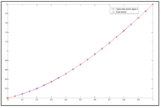
Figure 12. The exact solution $y_e\left(x\right)$ (represented by circles with dashed lines) and the approximate solution $y_a\left(x\right)$ (represented by stars with dashed lines) for degree 4.

6.4. Example 4: A Non-Homogeneous 2nd Order Linear ODE with BVP [36]

$$\begin{array}{ll}& y^{″}-2y^{\prime }+y=x{e}^x+4,\\ \mathrm{with} & y\left(0\right)=1, y\left(1\right)=2.\end{array}$$

The exact solution of the above problem is

$$y_e\left(x\right)={\displaystyle \frac{1}{6}}\left(x^3{e}^x+17x{e}^x-18e^x\right)-2x{e}^{\left(x-1\right)}+4.$$

Firstly, suppose the approximate solution is the Said–Ball curve of degree 3.

$$y_a\left(x\right)=S_a\left(x\right)=\sum _{j=0}^3{S}_j^m\left(x\right)v_j=v_0{S}_0^3\left(x\right)+v_1{S}_1^3\left(x\right)+v_2{S}_2^3\left(x\right)+v_3{S}_3^3\left(x\right),$$

$$=v_0{\left(1-x\right)}^2+2v_{1}x{\left(1-x\right)}^2+2v_2{x}^2\left(1-x\right)+v_3{x}^2.$$

(28)

The values of the Said–Ball curve’s control points were determined using the proposed method, along with the given conditions y (0) = 0 and y (1) = 2, after resolving the constrained optimization problem (see Table 8).

Table 8. Control points values of the Said–Ball curves of degree 3.

Control Points	Values
$v_0$	0.9999999941
$v_1$	0.5627636123
$v_2$	−0.5020055626
$v_3$	2.0000000006

By substituting the calculated values of the control points of the Said–Ball curve into (28), the approximate solution of the BVP for the 2nd-order non-homogeneous ODE is obtained. Therefore, the approximate solution of degree 3 is given in Equation (29).

$$\begin{array}{ll}{y}_a\left(x\right)=S_a\left(x\right)=& 0.9999999941{\left(1-x\right)}^2+1.1255272246x{\left(1-x\right)}^2\\ & -1.0040111252x^2\left(1-x\right)+2.0000000006x^2.\end{array}$$

(29)

Figure 13 shows the approximate and exact solutions graphically.

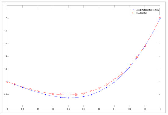
Figure 13. The exact solution $y_e\left(x\right)$ (represented by circles with dashed lines) and the approximate solution $y_a\left(x\right)$ (represented by stars with dashed lines) for degree 3.

Thus, the error accuracy between the exact and approximate solutions does not meet the expected level. Therefore, by increasing the degree of the Said–Ball curve to 4.

$$\begin{array}{ll}{y}_a\left(x\right)=S_a\left(x\right)=& {\displaystyle \sum _{j=0}^4}{S}_j^m\left(x\right)v_j\\ & =v_0{S}_0^4\left(x\right)+v_1{S}_1^4\left(x\right)+v_2{S}_2^4\left(x\right)+v_3{S}_3^4\left(x\right)+v_4{S}_4^4\left(x\right),\\ y_a\left(x\right)=S_a\left(x\right)=& v_0{\left(1-x\right)}^3+3v_{1}x{\left(1-x\right)}^3+6v_2{x}^2{\left(1-x\right)}^2\\ & +3v_3{x}^3\left(1-x\right)+v_4{x}^3.\end{array}$$

(30)

The control points values of the Said–Ball curve in Table 9 were calculated by applying the proposed method with the boundary conditions $y\left(0\right)=1 \mathrm{a}\mathrm{n}\mathrm{d} y\left(1\right)=2$.

Table 9. Control points values of the Said–Ball curve for Example 4.

Control Points	Values
$v_0$	0.9999999995
$v_1$	0.6991391125
$v_2$	0.6742822767
$v_3$	0.3137076492
$v_4$	1.9999999680

Thus, the approximate solution is computed by substituting the values of the control points into (30). Consequently, the approximate solution of degree 4, using the LSM with the Said–Ball curve, is as follows:

$$\begin{array}{ll}{y}_a\left(x\right)=S_a\left(x\right)=& 0.9999999995{\left(1-x\right)}^3+2.0974173375x{\left(1-x\right)}^3+4.0456936602x^2{\left(1-x\right)}^2\\ & +0.9411229476x^3\left(1-x\right)+1.9999999680x^3.\end{array}$$

The approximate solution of degree 4 and the exact solution are presented graphically in Figure 14.

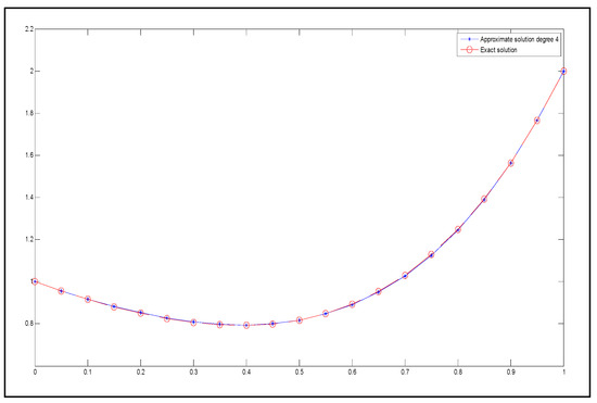
Figure 14. The exact solution $y_e\left(x\right)$ (represented by circles with dashed lines) and the approximate solution $y_a\left(x\right)$ (represented by stars with dashed lines) for degree 4.

7. Results and Discussion

The Said–Ball curve is used as a basis function for program development in the mathematical software MATLAB. The approximate solutions for BVPs, including second-order and fourth-order ODEs as well as second-order non-homogeneous ODEs, are computed using the Said–Ball curve with the LSM.

The following tables present the highest absolute error, highest relative error, and highest percentage relative error between the exact and approximate solutions based on the Said–Ball curves. These results are compared with existing methods, including the Bézier curve [30], the direct inverse method, the steepest descent method, and FMARI [36] (see Table 10, Table 11, Table 12, Table 13, Table 14, Table 15 and Table 16).

Table 10. Comparison of the maximum errors between the proposed method and the existing study (Bézier curve) for problem 2.

Errors	Bézier Curve [30]	Proposed Method	Error Accuracy Improved
Max Absolute Error	0.0000205000	0.0000030955	0.0000174040
Max Relative Error	0.0696930856	0.0012276801	0.0684654055
Max Percent Relative Error	6.9693085614	0.1227680090	6.8465405524

Table 11. Comparison of the maximum errors between the proposed method and the existing study (direct inverse method) for problem 3.

Errors	Direct Inverse Method [36]	Proposed Method	Error Accuracy Improved
Max Absolute Error	0.0108610200	0.0011377431	0.0097232769
Max Relative Error	0.0352655193	0.0052109784	0.0300545409
Max Percent Relative Error	3.5265519267	0.5210978390	3.0054540877

Table 12. Comparison of the maximum errors between the proposed method and the existing study (steepest descent method) for problem 3.

Errors	Steepest Descent Method [36]	Proposed Method	Error Accuracy Improved
Max Absolute Error	0.0108073000	0.0011377431	0.0096695569
Max Relative Error	0.0349771397	0.0052109784	0.0297661613
Max Percent Relative Error	3.4977139730	0.5210978390	2.976616134

Table 13. Comparison of the maximum errors between the proposed method and the existing study (FMARI) for problem 3.

Errors	FMARI [36]	Proposed Method	Error Accuracy Improved
Max Absolute Error	0.0103579380	0.0011377431	0.0092201949
Max Relative Error	0.0325642234	0.0052109784	0.027353245
Max Percent Relative Error	3.2564223426	0.5210978390	2.7353245036

Table 14. Comparison of the maximum errors between the proposed method and the existing study (direct inverse method) for problem 4.

Errors	Direct Inverse Method [36]	Proposed Method	Error Accuracy Improved
Max Absolute Error	0.0521528400	0.0030998110	0.0490530290
Max Relative Error	0.0638078279	0.0038462689	0.0599615590
Max Percent Relative Error	6.380782789	0.3846268926	5.9961558964

Table 15. Comparison of the maximum errors between the proposed method and the existing study (steepest descent method) for problem 4.

Errors	Steepest Descent Method [36]	Proposed Method	Error Accuracy Improved
Max Absolute Error	0.0521528720	0.0030998110	0.0490530610
Max Relative Error	0.0638078670	0.0038462689	0.0599615981
Max Percent Relative Error	6.3807867046	0.3846268926	5.9961598120

Table 16. Comparison of the maximum errors between the proposed method and the existing study (FMARI) for problem 4.

Errors	FMARI [36]	Proposed Method	Error Accuracy Improved
Max Absolute Error	0.0521528210	0.0030998110	0.04905301
Max Relative Error	0.0638078046	0.0038462689	0.0599615357
Max Percent Relative Error	6.3807804649	0.3846268926	5.9961535723

The above tables show that the proposed method significantly improves error accuracy.

8. Conclusions

In this study, Said–Ball curves are represented using the LSM to approximate solutions for higher-order ODEs. The approximate solution is expressed as Said–Ball curves and substituted into the given ODEs. We determined the optimal control points of Said–Ball curves by minimizing the residual error, defined as the sum of the squares of the residual function. A better approximate solution was obtained by applying these optimized control points to the Said–Ball curves, significantly improving error accuracy compared to existing methods.

The computation process is straightforward and does not require external directional controls. Numerical examples of linear and non-homogeneous linear ODEs are provided to demonstrate the effectiveness of Said–Ball curve representations. Additionally, we developed an algorithm and performed a convergence analysis for two-point boundary value problems based on the control points of Said–Ball curves using the LSM. The proposed method is versatile and can be applied to solve other types of differential equations.

References

- Lai, M.J.; Wenston, P. Bivariate spline method for numerical solution of steady state Navier–Stokes equations over polygons in stream function formulation. Numer. Methods Partial. Differ. Equ. Int. J. 2000, 16, 147–183. [Google Scholar] [CrossRef]
- Nürnberger, G.; Zeilfelder, F. Developments in bivariate spline interpolation. J. Comput. Appl. Math. 2000, 121, 125–152. [Google Scholar] [CrossRef]
- Mortari, D. Least-squares solution of linear differential equations. Mathematics 2017, 5, 48. [Google Scholar] [CrossRef]
- Adiyaman, M.; Oger, V. A residual method using Bezier curves for singular nonlinear equations of Lane-Emden type. Kuwait J. Sci. 2017, 44, 9–18. [Google Scholar]
- Al-Janabi, A.N.; Al Zahed, F.J.; Hussain, A.H. An approximate solution of integral equation using Bezier control points. Int. J. Nonlinear Anal. Appl. 2021, 12, 793–798. [Google Scholar]
- Jameel, A.F.; Amen, S.G.; Saaban, A.; Man, N.H. On solving fuzzy delay differential equation using Bezier curves. Int. J. Electr. Comput. Eng. 2020, 10, 6521–6530. [Google Scholar] [CrossRef]
- Ayoo, P.V.; Amobeda, R.E.; Akinwale, O. Solution of systems of disjoint Fredholm-Volterra integro-differential equations using Bezier control points. Sci. World J. 2020, 15, 35–40. [Google Scholar]
- Ghomanjani, F.; Farahi, M.H.; Pariz, N. A new approach for numerical solution of a linear system with distributed delays, Volterra delay-integro-differential equations, and nonlinear Volterra-Fredholm integral equation by Bezier curves. Comput. Appl. Math. 2017, 36, 1349–1365. [Google Scholar] [CrossRef]
- Gachpazan, M. Solving of time varying quadratic optimal control problems by using Bézier control points. Comput. Appl. Math. 2011, 30, 367–379. [Google Scholar] [CrossRef][Green Version]
- Beltran, J.V.; Monterde, J. Bézier solutions of the wave equation. In Proceedings of the International Conference on Computational Science and Its Applications, Assisi, Italy, 14–17 May 2004; pp. 631–640. [Google Scholar]
- Farin, G. Curves and Surfaces for Computer Aided Geometric Design-A Practical Guide, 4th ed.; Rheinbolt, W., Ed.; Academic Press: San Diego, CA, USA, 1997. [Google Scholar]
- Ball, A.A. CONSURF. Part one: Introduction of conic lofting tile. Comput. Aided Des. 1974, 6, 243–249. [Google Scholar] [CrossRef]
- Ball, A.A. CONSURF. Part two: Description of the algorithms. Comput. Aided Des. 1975, 7, 237–242. [Google Scholar] [CrossRef]
- Ball, A.A. CONSURF. Part three: How the program is used. Comput. Aided Des. 1977, 9, 9–12. [Google Scholar] [CrossRef]
- Said, H.B. A generalized Ball curve and its recursive algorithm. ACM Trans. Graph. 1989, 8, 360–371. [Google Scholar] [CrossRef]
- Wang, G. Ball curve of high degree and its geometric properties. Appl. Math. A J. Chin. Univ. 1987, 2, 126–140. [Google Scholar]
- Hongyi, W. Unifying representation of Bézier curve and generalized Ball curves. Appl. Math. J. Chin. Univ. 2000, 15, 109–121. [Google Scholar] [CrossRef]
- Goodman, T.N.; Said, H.B. Properties of generalized Ball curves and surfaces. Comput. Aided Des. 1991, 23, 554–560. [Google Scholar] [CrossRef]
- Delgado, J.; Pena, J.M. A linear complexity algorithm for the Bernstein basis. In Proceedings of the 2003 International Conference on Geometric Modeling and Graphics, London, UK, 16–18 July 2003; IEEE: New York, NY, USA, 2003. [Google Scholar]
- Delgado, J.; Peña, J.M. A shape preserving representation with an evaluation algorithm of linear complexity. Comput. Aided Geom. Des. 2003, 20, 1–10. [Google Scholar] [CrossRef]
- Aphirukmatakun, C.; Dejdumrong, N. Multiple degree elevation and constrained multiple degree reduction for DP curves and surfaces. Comput. Math. Appl. 2011, 61, 2296–2299. [Google Scholar] [CrossRef][Green Version]
- Hu, S.M.; Wang, G.Z.; Jin, T.G. Properties of two types of generalized Ball curves. Comput. Aided Des. 1996, 28, 125–133. [Google Scholar] [CrossRef]
- Pihien, H.N.; Dejdumrong, N. Efficient algorithms for Bézier curves. Comput. Aided Geom. Des. 2000, 17, 247–250. [Google Scholar]
- Jaafar, W.; Nurhadani, W. Visualization of Curve and Surface Data Using Rational Cubic Ball Functions. Ph.D. Thesis, Universiti Sains Malaysia, Pulau Pinang, Malaysia, 2018. [Google Scholar]
- Weierstrass, K. Über die analytische Darstellbarkeit sogenannter willkürlicher Functionen einer reellen Veränderlichen. Sitzungsberichte Der Königlich Preußischen Akad. Der Wiss. Zu Berl. 1885, 2, 633–639. [Google Scholar]
- Lambert, J.D.; Watson, I.A. Symmetric multistip methods for periodic initial value problems. IMA J. Appl. Math. 1976, 18, 189–202. [Google Scholar] [CrossRef]
- Sarafyan, D. New algorithms for the continuous approximate solutions of ordinary differential equations and the upgrading of the order of the processes. Comput. Math. Appl. 1990, 20, 77–100. [Google Scholar] [CrossRef]
- Anake, T.A. Continuous Implicit Hybrid One-Step Methods for the Solution of Initial Value Problems of General Second-Order Ordinary Differential Equations. Ph.D. Thesis, Covenant University, Ogun State, Nigeria, 2011. [Google Scholar]
- Ascher, U. Discrete least squares approximations for ordinary differential equations. SIAM J. 1978, 15, 478–496. [Google Scholar] [CrossRef]
- Zheng, J.; Sederberg, W.T.; Johnson, W.R. Least squares methods for solving differential equations using Bezier control points. Appl. Numer. Math. 2004, 48, 237–252. [Google Scholar] [CrossRef]
- Yousef, F.; Alkam, O.; Saker, I. The dynamics of new motion styles in the time-dependent four-body problem: Weaving periodic solutions. Eur. Phys. J. Plus 2020, 135, 742. [Google Scholar] [CrossRef]
- Yousef, F.; Semmar, B.; Al Nasr, K. Incommensurate conformable-type three-dimensional Lotka–Volterra model: Discretization, stability, and bifurcation. Arab. J. Basic Appl. Sci. 2022, 29, 113–120. [Google Scholar] [CrossRef]
- Amaal, A.M. Approximate solution of differential equations of fractional orders using Bernstein-Bézier polynomial. Al-Mustansiriya J. Sci. 2012, 23, 65–74. [Google Scholar]
- Alavizadeh, S.R.; Maalek, G.F. Numerical solution of higher-order linear and nonlinear ordinary differential equations with orthogonal rational legendre functions. J. Math. Ext. 2014, 8, 109–130. [Google Scholar]
- Monterde, J. Bézier surfaces of minimal area: The Dirichlet approach. Comput. Aided Geom. Des. 2004, 21, 117–136. [Google Scholar] [CrossRef]
- Jameel, A.F.; Anakira, N.R.; Shather, A.H.; Saaban, A.; Alomari, A.K. Numerical algorithm for solving second order nonlinear fuzzy initial value problems. Int. J. Electr. Comput. Eng. 2020, 10, 6497–6506. [Google Scholar] [CrossRef]
- Hunter, J. Continuous Functions. Available online: https://www.math.ucdavis.edu/~hunter/book/ch2.pdf (accessed on 21 July 2005).
- Casselman, B. From Bézier to Bernstein; Feature Column from American Mathematical Society: Providence, RI, USA, 2008. [Google Scholar]
- Bhatti, A.; Karim, S.B. Approximation method using DP Ball curves for solving ordinary differential equations. Math. Stat. 2023, 11, 464–489. [Google Scholar] [CrossRef]
- Ghomanjani, F. A new approach for solving linear fractional integro-differential equations and multi variable order fractional differential equations. Proyecciones 2020, 39, 199–218. [Google Scholar] [CrossRef]
- Ibrahim, S. Numerical approximation method for solving differential equations. Eur. J. Sci. Eng. 2020, 6, 157–168. [Google Scholar]
- Aphirukmatakun, C.; Dejdumrong, N. An approach to polynomial curve comparison in geometric object database. Int. J. Comput. Sci. 2007, 2, 240–246. [Google Scholar]
- Dan, Y.; Xinmeng, C. Another type of generalized ball curves and surfaces. Acta Math. Sci. 2007, 27, 897–907. [Google Scholar] [CrossRef]
Disclaimer/Publisher’s Note: The statements, opinions and data contained in all publications are solely those of the individual author(s) and contributor(s) and not of MDPI and/or the editor(s). MDPI and/or the editor(s) disclaim responsibility for any injury to people or property resulting from any ideas, methods, instructions or products referred to in the content. |
© 2025 by the authors. Licensee MDPI, Basel, Switzerland. This article is an open access article distributed under the terms and conditions of the Creative Commons Attribution (CC BY) license (https://creativecommons.org/licenses/by/4.0/).