Abstract
This study aims to investigate various dynamical aspects of the dual-mode Gardner equation derived from an ideal fluid model. By applying a specific wave transformation, the model is reduced to a planar dynamical system, which corresponds to a conservative Hamiltonian system with one degree of freedom. Using Hamiltonian concepts, phase portraits are introduced and briefly discussed. Additionally, the conditions for the existence of periodic, super-periodic, and solitary solutions are summarized in tabular form. These solutions are explicitly constructed, with some graphically represented through their and profiles. Furthermore, the influence of specific physical parameters on these solutions is analyzed, highlighting their effects on amplitude and width. By introducing a more general periodic external influence into the model, quasi-periodic and chaotic behavior are explored. This is achieved through the presentation of and phase portraits, along with time-series analyses. To further examine chaotic patterns, the Poincaré surface of section and sensitivity analysis are employed. Numerical simulations reveal that variations in frequency and amplitude significantly alter the dynamical characteristics of the system.
Keywords:
dual-mode Gardner equation; phase portrait; wave solutions; quasi-periodic; chaotic behavior MSC:
35C07; 35C08; 37K40; 83C15
1. Introduction
In mechanical engineering, nonlinear partial differential equations (PDEs) are crucial because they describe intricate processes, such as heat transfer, fluid flow, material stress, and deformation. Nonlinear PDEs are generally more difficult to solve and, due to their complexity, typically require numerical or approximate methods, in contrast to linear PDEs, which often have analytical solutions [1,2]. Finding exact solutions to such equations is important because it allows us to understand and explain many complex phenomena modeled by these equations. As a result, researchers are motivated to explore new methods or refine existing ones. Various powerful methods have been proposed and successfully applied in several works, such as the inverse scattering transform [3], Hirota’s bilinear operators [4,5], the Bäcklund–Darboux transform [6,7,8], the homotopy perturbation method [9], projective Riccati equations [10], the sub-ODE method [11,12], Lie symmetry [13,14,15,16,17,18], the auxiliary equation technique [19,20], the Kudryshov technique [21], Painlevé analysis [22,23], and bifurcation analysis [24,25,26,27,28,29].
Surface waves in shallow water have been extensively studied due to their distinctive characteristics. These waves are commonly described using mathematical models, with the Korteweg–de Vries (KdV) equation being one of the fundamental formulations. The KdV equation is particularly notable for its well-defined solutions and plays a crucial role in analyzing the dynamics of shallow-water waves [30]. Its origin is linked to its development as a nonlinear wave equation governing unidirectional wave propagation [30]. This equation was derived through an asymptotic expansion of the fundamental wave motion within the shallow-water Euler equations, closely related to the study of small-amplitude waves on a free surface. It encompasses two significant parameters, and , which define the wave size relative to the water depth and the square of the water depth relative to the wavelength, respectively. Thus, the KdV equation incorporates two essential elements: linear dispersion, which explains the spreading and transformation of waves, and nonlinear steepening, where waves grow taller in shallow water [31]. This equation is crucial for understanding the behavior of solitary waves in these contexts and for examining the characteristics of periodic waves, which aids in our comprehension of the consistent patterns and oscillations observed in various wave phenomena. Now, here is the key point: this equation behaves differently when and have significantly different values. In other words, when the wave size differs from the water depth, it significantly affects how these waves move and behave. Equations that account for higher-order effects, such as higher-order KdV equations, follow the same principle [31]. The derivation of this equation originates from the (2 + 1)-dimensional Gardner equation [32], which illustrates the relationship between the sizes of and : and , where is the transverse wavelength parameter.
It is important to highlight that in our research, we are focusing on a specific case with a flat bottom, which requires setting the bottom variation parameter equal to zero. This choice is particularly significant because it simplifies our calculations. Our study focuses on the Gardner equation, which was originally derived in a previous work [33]:
Equation (1) is essential to the analysis and is employed to examine the behavior of a specific non-dimensional parameter: the Bond number , , and , where , and L define the average upstream depth, gravity acceleration, wave amplitude, surface tension coefficient, water density, and wave length, respectively. These non-dimensional factors are crucial to our investigation because they enable us to understand the behavior of the system under consideration. The Korsunsky approach [34] is applied to transform Equation (1) into a novel dual-mode model, as presented in [35]. Thus, we obtain the following dual-mode model for the Gardner equation:
where represents a field function defined over the domain . Here, and denote the nonlinearity parameter and dispersion, respectively, and are restricted by and , while s characterizes the phase velocity. The dual-mode Gardner equation generalizes both the KdV equation and the modified KdV (mKdV) equation by incorporating both quadratic and cubic nonlinear terms. It is widely used to model the propagation of nonlinear waves in various physical systems, especially in fields such as fluid dynamics and plasma physics [36,37]. It is worth mentioning that the Korsunsky approach has been extended to the KdV equation by several scholars to investigate dual-mode equations. For instance, the dual-mode modified KdV and higher order KdV equations were studied in [38], the dual-mode Kuramoto–Sivashinsky equation was investigated in [39,40], and the dual-mode Sharma–Tasso–Olver equation and the dual-mode fourth-order Burgers equation were considered in [41]. Soliton solutions of Equation (2) were constructed utilizing the tan/cot and tanh/coth methods in [35]. Lie symmetry analysis has been applied to Equation (2), and some solutions have been obtained using the power series method [42].
The primary objectives of this work are to apply the qualitative theory of planar systems to determine and systematically tabulate the existence conditions for certain bounded solutions to Equation (2) and to explicitly construct some of these solutions. Additionally, we analyze the influence of specific physical parameters on these solutions. Furthermore, by incorporating external periodic effects into the model, we investigate the emergence of quasi-periodic and chaotic behavior in wave phenomena.
This work is organized as follows. In Section 2, we apply a specific wave transformation to convert Equation (2) into a dynamical system that is equivalent to a Hamiltonian system with one degree of freedom. Section 3 focuses on the bifurcation analysis of the traveling wave system, including the tabulation of the existence conditions for periodic, super-periodic, and solitary solutions, along with a brief description of the phase portrait. In Section 4, we construct specific solutions categorized as periodic, super-periodic, and solitary. Section 5 presents graphical representations of some solutions in both and formats, as well as an analysis of the influence of certain physical parameters on these solutions. In Section 6, we examine quasi-periodic and chaotic behavior by introducing an external periodic perturbation term. A sensitivity analysis for different initial conditions is conducted, and Poincaré section and bifurcation diagrams are used to identify chaotic patterns in the model. Finally, Section 7 summarizes the key findings of this study.
2. Traveling Wave System
Let us assume that the solution to Equation (2) is expressed as follows:
where is the wave variable, represents the wave number, and denotes the wave speed. The solution form (3) stands for the traveling wave solution to Equation (2). By substituting Equation (3) into Equation (2), we obtain
where ’ indicates the derivatives with respect to . By integrating Equation (4) twice with respect to and setting the integration constants to zero, we derive
where are newly introduced constants for simplicity, replacing the original ones, and are given by
Let and let . Then, the second-order differential Equation (5) is written as follows:
The system in Equation (7a,b) is referred to as the traveling wave system. It is conservative because , and it is Hamiltonian because it can be derived from the Hamiltonian function
using Hamilton’s canonical equations [43], where is the three-parameter potential function given by
The Hamiltonian function itself is a constant of motion for the system in Equation (7a,b), as it does not explicitly depend on [43]. Hence, we have
where q is a free parameter that will play a key role in the subsequent analysis, as we demonstrate later. Substituting Equation (7a) into the conserved quantity (10) and separating the variables, we obtain the following differential form:
where is a quartic polynomial taking the form
Since one of the main objectives is to construct all possible solutions to Equation (2), determining the range of the parameters , and q is essential for integrating the differential form (11). The qualitative theory for planar integrable systems is applied to identify this range. Furthermore, this approach is significant because it does not only provide the required parameter ranges but also determines the type of solutions before solving them by linking them with phase trajectories. This enables us to isolate bounded solutions, which are physically meaningful, and to construct only real (non-complex) solutions by introducing the concept of intervals for real wave propagation.
3. Bifurcation and Phase Portrait
The dynamical behavior and qualitative analysis of Equation (2) are explored using Hamiltonian concepts [43,44]. The significance of the bifurcation study is encapsulated in the following lemma, which is crucial, as it illustrates the relationship between the phase trajectories and the types of solutions.
Lemma 1
([45,46]). Assume that is a solution to Equation (2) for all with and . Hence, Equation (2) possesses the following:
- (a)
- A solitary solution corresponding to a homoclinic trajectory when .
- (b)
- A kink (or anti-kink) solution corresponding to a heteroclinic trajectory when .
- (c)
- A periodic solution corresponding to the periodic phase trajectory.
On the other hand, unbounded phase trajectories are linked to unbounded solutions, which are physically undesirable in real-world problems. Consequently, the bifurcation study allows us to disregard such solutions associated with these trajectories. Hence, the bifurcation analysis is necessary for determining the range of the parameters and q in order to integrate both sides of the differential form in Equation (11). Additionally, it is essential to find the conditions on these parameters that lead to periodic, homoclinic, heteroclinic, and unbounded trajectories.
The phase portrait of the system in Equation (7a,b) can vary depending on the number of equilibrium points and the number of separatrix layers it covers [47]. To systematize the distinct trajectories in the phase portrait, we denote the periodic trajectory, heteroclinic trajectory, homoclinic trajectory, and super-nonlinear periodic trajectory as , , , and , where p represents the number of stable equilibrium points covered by the trajectory and r denotes the number of separatrix layers covered by the trajectory [48].
Let us first introduce the following theorem, which will be useful for the subsequent analysis.
Theorem 1
((Lagrange Theorem) [44]). For a conservative system, if the potential energy has a strict minimum at some positions, then these positions are stable equilibrium points.
Let us assume and define as the equilibrium point of the system in Equation (7a,b), where is a critical point of the potential function in Equation (9), i.e., a solution to the equation
The number of equilibrium points depends on the value of , which can be negative, zero, or positive. We examine each case individually:
- 1.
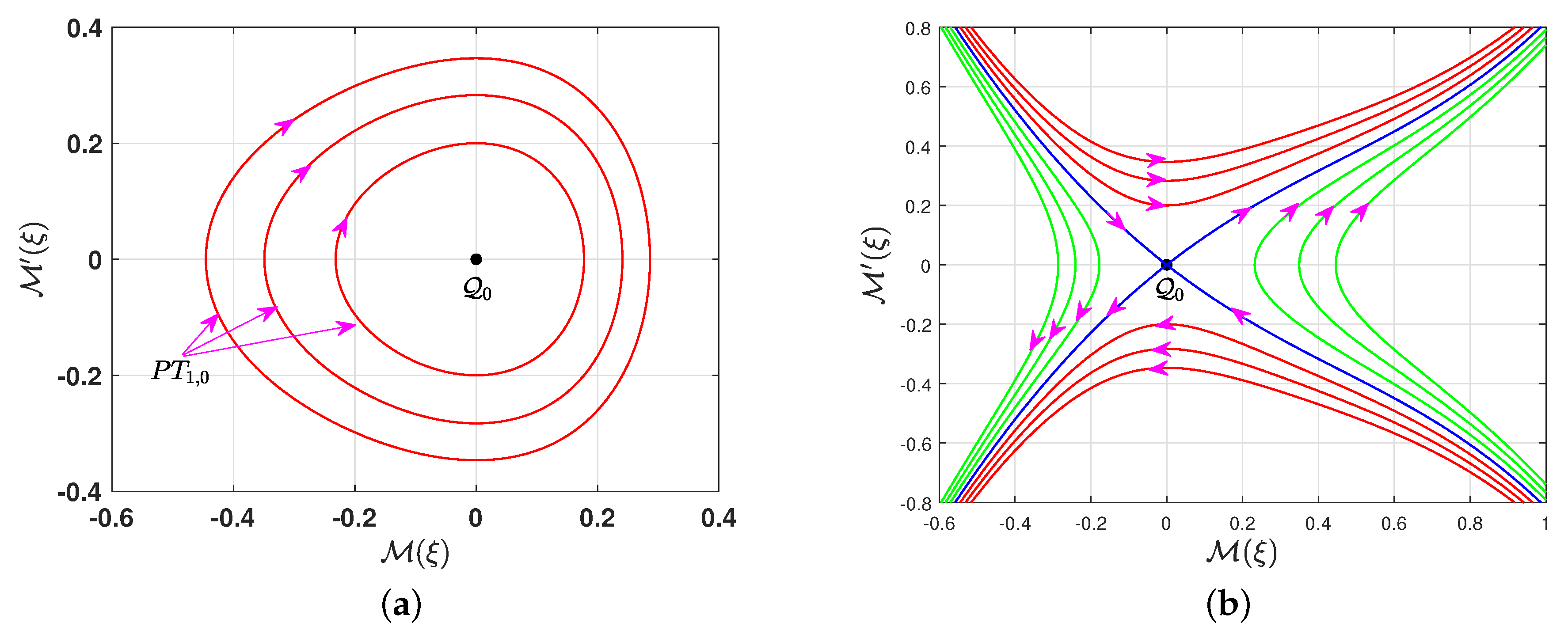
- If , which is equivalent to , then Equation (13) has a unique solution, . Consequently, the system in Equation (7a,b) has a single equilibrium point, . To classify the nature of this point, we apply Theorem 1. Direct calculations yield . The point is classified as either a center point if or a saddle point if . The value of the parameter q at the equilibrium point is calculated, resulting in . Figure 1 illustrates the phase portrait of the system (7a,b) for , representing the scenario in which the system has a single equilibrium point. We conclude that when , all phase trajectories of the system are bounded and periodic, and are classified as for all , as depicted in Figure 1a. Conversely, when , all phase trajectories of the system (7a,b) are unbounded for all possible values of .
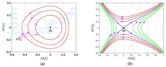 Figure 1. The phase portrait of the system (7a,b) for . The black point marks the equilibrium point. (a) , (b) .
 - 2.
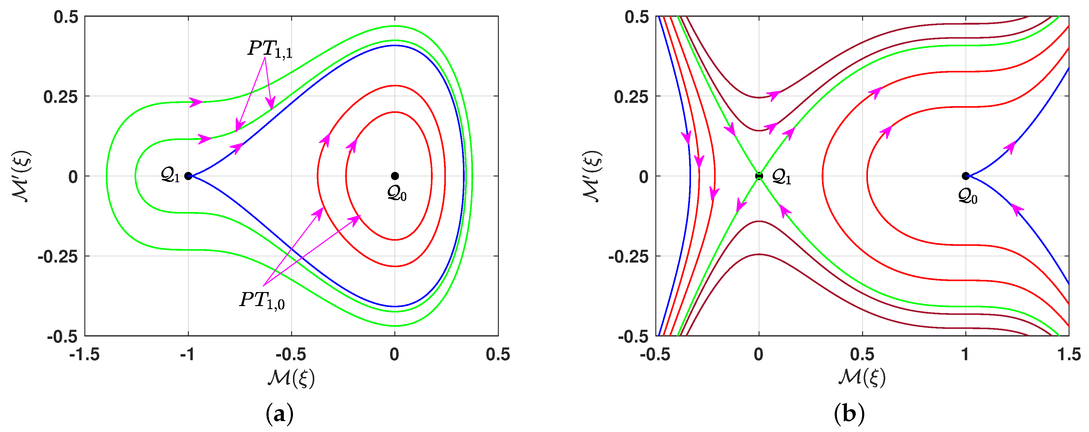
- When , this condition corresponds to , where . In this case, Equation (13) yields two solutions: and . As a result, the system (7a,b) possesses two equilibrium points: and . Theorem 1 is applied to classify these points. Direct calculations yieldHence, the equilibrium point is a cusp point, and is a center point if or a saddle point if . The phase portrait for the system (7a,b) in this case is shown in Figure 2. We compute the value of the parameter q at the following equilibrium points: and . We briefly describe the phase portrait in this case. When , all phase trajectories are bounded and periodic, varying according to the values of the parameter q, as shown in Figure 2a. There are two families of periodic trajectories: one characterized by for in green, and the other by for in red. Additionally, the blue trajectory passing through the cusp point typically exhibits periodic behavior, especially near the equilibrium point. On the other hand, if , all phase trajectories of the system (7a,b) are unbounded, as shown in Figure 2b.
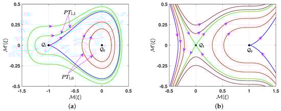 Figure 2. The phase portrait of the system (7a,b) for . The black point marks the equilibrium point. (a) , (b) .
 - 3.
- If , which is equivalent to , then Equation (13) has three real solutions, . Consequently, the system (7a,b) has three equilibrium points: and . The Lagrange Theorem 1 is employed to classify the equilibrium points; hence, we haveAlso, we compute the value of q at the following points:which are sufficient to give a short description of the phase portrait. Let us now consider the next two cases, in which is either positive or negative:
- Case A: If , the condition yields or :
- (a)
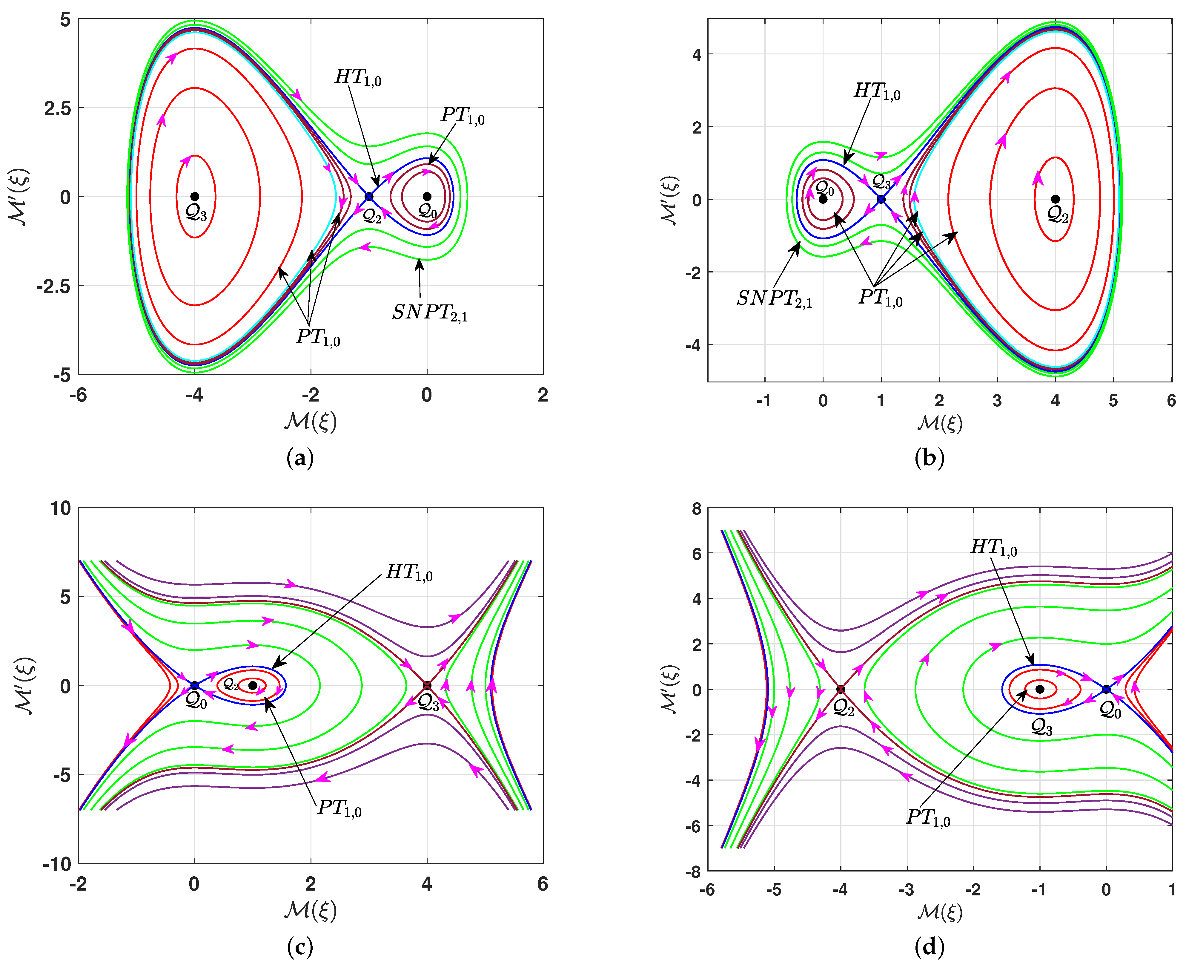
- If , and , the equilibrium point is a center point, while is a saddle point and is a center point. Figure 3a depicts the phase portrait for the system (7a,b) in this case. It consists of several types of bounded trajectories, depending on the values of the parameter q. There is a family of super-periodic trajectories in green, characterized by for , two brown families of periodic trajectories around the center point , characterized by for , a family of red periodic trajectories around the center point , characterized by for , and a single cyan periodic trajectory for . Additionally, there are two homoclinic trajectories in blue for , which is characterized by .
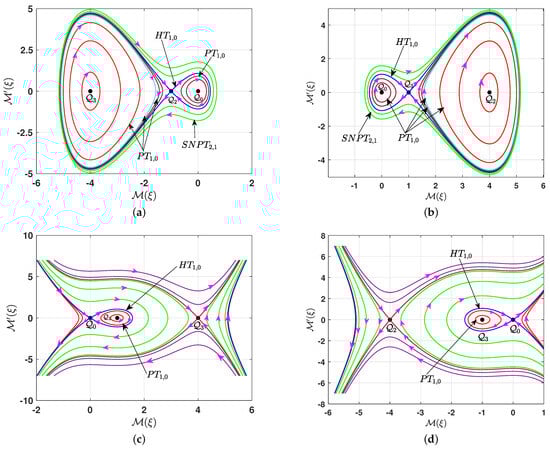 Figure 3. The phase portrait of the system (7a,b) for with . The black point marks the equilibrium point. (a) , (b) , (c) , (d) .
 - (b)
- On the other hand, if , and , then is a center point, is a center point, and is a saddle point. The phase portrait for this case is shown in Figure 3b. All the trajectories are bounded and categorized into different types based on the value of the parameter q. A similar phase description can be provided as in (a).
- (c)
- If , and , the equilibrium point is a saddle point, while is a center point and is a saddle point. The phase portrait for this case is illustrated in Figure 3c. All the phase trajectories are unbounded, except for the family of periodic red trajectories for , which is characterized by . This family is enclosed within a homoclinic trajectory in blue for , which is characterized by .
- (d)
- If , and , the equilibrium point is a saddle point, while is a saddle point and is a center point. The phase portrait for this case is shown in Figure 3d. A similar phase description can be provided as in (c).
- Case B: If , then the condition holds automatically. Thus, we proceed to consider the following possible cases:
- (a)
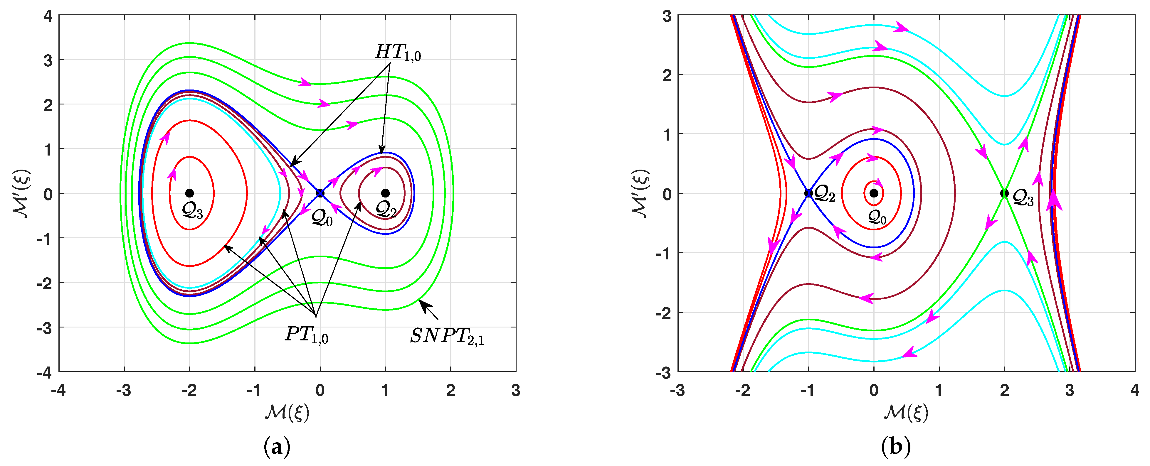
- If , and is a nonzero real number, the equilibrium point is a saddle point while and are center points. The phase portrait for the system (7a,b) corresponding to this case is illustrated in Figure 4a. All the phase trajectories are bounded, and their type depends on the value of the parameter q. There is a family of periodic red trajectories around the center point for , and two periodic families of brown trajectories surrounding the two center points and for , situated within the two homoclinic orbits (blue) at . Additionally, there is a single periodic trajectory (cyan) for . All these periodic trajectories are characterized by . Furthermore, for , there is a green family of super-periodic trajectories characterized by .
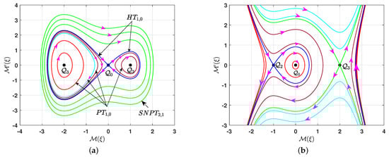 Figure 4. The phase portrait of the system (7a,b) for with . The black point marks the equilibrium point. (a) , (b) .
 - (b)
- If , and is a nonzero real number, the equilibrium point is a center point while both equilibrium points are saddle points. The phase portrait for this case is depicted in Figure 4b. All the phase trajectories are unbounded, except for a family of red periodic trajectories around the center point when . This family lies within the homoclinic orbit (blue) at .
4. Solutions
According to Lemma 1, the nature of the solution depends on the characteristics of the trajectories. Therefore, it is more appropriate to compile and tabulate the conditions that result in periodic, super-periodic, and solitary solutions. Unbounded solutions are excluded, as they are physically unacceptable. Hereafter, we compute the solutions corresponding to similar trajectories where the leading term of the polynomial (12) has the same sign.
4.1. Periodic Solutions
This subsection constructs periodic solutions to Equation (2), utilizing the parameter restrictions summarized in Table 1. Thus, we have the following:

Table 1.
Conditions for the existence of periodic solutions to Equation (2).
- (a)
- The parameter conditions in Case 1 indicate that the polynomial (12) has two real roots, denoted as , where , and two complex conjugate roots, denoted as , where * denotes the complex conjugate. Thus, it can be expressed as . The interval for the real solution is . Assuming , integrating both sides of Equation (11) yields a new solution to Equation (2) of the formwhere , , and . The solution (15) is periodic, with a period given by , where denotes the complete elliptic integral of the first kind [49].The solutions corresponding to Case 2, Case 3, Case 5, Case 7, and Case 12 in Table 1 are identical to the solution (15), differing only in their arguments. This difference arises because the roots of the polynomial change with the parameter constraints, while the sign of the leading order of the polynomial remains fixed.
- (B)
- The parameter conditions in Case 4, Case 8, and Case 13 indicate that the polynomial (12) has four real zeros, denoted as for , satisfying . Thus, it is written as . The intervals of the real solutions are . For , we assume and integrate both sides of Equation (11). Consequently, we obtain a novel periodic solution to Equation (2) of the formwhere . The period of the solution (16) is , where is a complete elliptic integral of the first kind [49]. The solution (16) corresponds to the left family of periodic trajectories, as illustrated in Figure 3a,b. On the other hand, if , we assume that . Consequently, integrating both sides of Equation (11) yieldswhich is a new periodic solution to Equation (2) with period . The solution (17) corresponds to the right family of periodic trajectories, as shown in Figure 3a,b.Note that for fixed values of the parameters , and q, two distinct solutions arise, depending on the differences in the intervals of real solutions. Hence, employing such intervals is crucial.
- (c)
- The parameter conditions in Case 6 and Case 9 indicate that the polynomial (12) has one double root at the origin and two simple roots given by . In Case 6, these roots satisfy , while in Case 9, . The polynomial (12) can be expressed as . The interval of real propagation is for Case 6 and for Case 9. Postulating in both cases and integrating both sides of Equation (11), we obtain
- (d)
- Cases 10, 11, and 15 justify the existence of four real zeros of the polynomial, namely , with . It is worth mentioning that the values of these roots vary from case to case due to their dependence on the polynomial coefficients. The polynomial (12) is expressed as . The intervals of the real solutions are given by . We restrict ourselves to , as this interval corresponds to periodic trajectories, whereas the other intervals describe unbounded trajectories. Integrating both sides of Equation (11) under the assumption (11) that yieldswhere . The solution (19) characterizes a new solution to Equation (2), with a period given by .
4.2. Super-Periodic Solutions
A super-periodic nonlinear wave, a novel type of nonlinear wave, is characterized by the nontrivial topology of its phase portraits, which exhibit greater complexity than simple periodic waves. These waves correspond to phase-plane orbits or trajectories that involve at least two stable equilibrium points (centers) and a separatrix layer. Super-periodic wave solutions arise in various physical phenomena, including fluid dynamics, optics, and plasma physics, where they play a crucial role in describing and predicting the evolution of wave patterns in complex systems. For further details on these solutions, see, for example, [50,51].
The conditions for the existence of super-periodic solutions to Equation (2) are summarized in Table 2. This section focuses on constructing these solutions.
Table 2.
Conditions for the existence of super-periodic solutions to Equation (2).
All cases in Table 2 demonstrate that the polynomial (12) has two real roots, and , with , and two complex conjugate roots, and . Consequently, the polynomial (12) can be expressed as . The interval of the real solutions is . Integrating both sides of Equation (11) under the assumption that yields
where , , and . Solution (20) characterizes a novel super-periodic solution to Equation (2).
4.3. Solitary Solutions
This subsection focuses on deriving the solitary wave solution to Equation (2), incorporating the parameter conditions specified in Table 3. For brevity, only selected cases are considered, as the calculations for the remaining cases follow a similar approach.
Table 3.
Conditions for the existence of solitary solutions to Equation (2).
First, we examine Case 1 in Table 3. In this case, the polynomial (12) has one double root, denoted by , which corresponds to the -coordinate of the saddle point . The other roots, , are simple. This implies that can be expressed as , where . The roots and are given by
The intervals for the real solutions are . The first interval, , corresponds to the left homoclinic trajectory, while the second interval, , corresponds to the right homoclinic trajectory, as illustrated by the blue curves in Figure 3b. Let us construct the solution corresponding to each interval individually:
- (a)
- (b)
Using similar calculations, we can construct the solution for Case 2 in Table 3.
Case 3 and Case 4 indicate that the polynomial (12) has a double root at the origin and two distinct simple roots, . For Case 3, these roots satisfy , whereas for Case 4, they satisfy . Accordingly, the polynomial (12) can be expressed as . The intervals of real wave propagation are for Case 3 and for Case 4. By integrating both sides of Equation (11) under the assumption that , we obtain the solution
which characterizes a novel solitary solution to Equation (2).
5. Physical Interpretation
This section focuses on graphically presenting some of the obtained solutions using and representations, as well as exploring the effects of the wave velocity and wave number on the periodic, super-periodic, and solitary solutions.
We allow the parameters to take the values , , , , , , , and . Consequently, Equation (6) yields , , and . It is evident that , , and . The phase portrait for the system (7a,b) is shown in Figure 3a. The values of the parameter q at the equilibrium points , , and are , , and , respectively. As mentioned above, the type of solution depends on the values of q, which also determine the nature of the trajectory.
If we select , then the system (7a,b) has two families of periodic orbits, shown in brown. The corresponding solution can be determined by calculating the roots , for , of the polynomial (12). These roots are , , , and . Consequently, the solution (16) becomes
Figure 5a and Figure 5b present the and representations of the solution (24), respectively, illustrating its periodicity. Additionally, we examine the influence of the wave velocity and wave number on the periodic solution (16) by fixing the values of all parameters while allowing only or to vary. Figure 5c demonstrates the impact of on the periodic solution (16), showing that as increases, the amplitude of the solution grows while its width decreases. Similarly, Figure 5d illustrates the effect of the wave number on the periodic solution (16). It is evident that as increases, the amplitude of the solution remains unchanged, while its width expands.
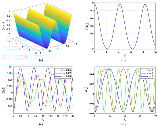
Figure 5.
Graphical representations of the periodic solution (16) and the influence of the wave velocity and wave number . (a) representation, (b) representation, (c) impact of , (d) impact of .
If we select , the system (7a,b) exhibits a family of super-periodic trajectories, shown in green in Figure 3b. Consequently, Equation (2) admits a solution of the form (20). To derive this solution, we calculate the roots of the polynomial (12), which are , , , and . Hence, the solution (20) is expressed as
Figure 6a,b present the and representations of the super-periodic solution (20), respectively. Figure 6c demonstrates that the effect of the wave velocity on the solution (20) is minimal for both amplitude and width. Figure 6d illustrates the influence of the wave number on the solution (20), showing that as increases, the amplitude of the solution remains nearly constant, while its width increases.
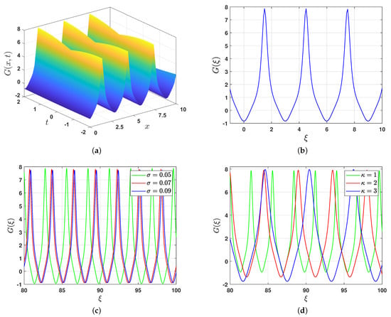
Figure 6.
Graphical representations of the super-periodic solution (20) and the influence of the wave velocity and wave number . (a) representation, (b) representation, (c) impact of , (d) impact of .
If we choose , the system (7a,b) has two homoclinic trajectories, as shown in Figure 3b. Hence, Equation (2) has a solitary solution of the form (21) or (22), depending on the possible intervals of the real solutions. To find these solutions, we first find the roots of the polynomial (12). These roots are , and . Hence, the solution (21) takes the form
Figure 7 provides a graphical representation of the solution (21). Specifically, Figure 7a,b show the and depictions of the solution, respectively. It is evident that this solution is symmetric about the vertical line , as illustrated in Figure 7b. Figure 7c demonstrates that the variation in the wave velocity has a minimal effect on the amplitude and width of the solution. Finally, Figure 7d highlights the influence of the wave number on the solution (21). As the wave number increases, the amplitude of the solution remains approximately constant, while its width expands.
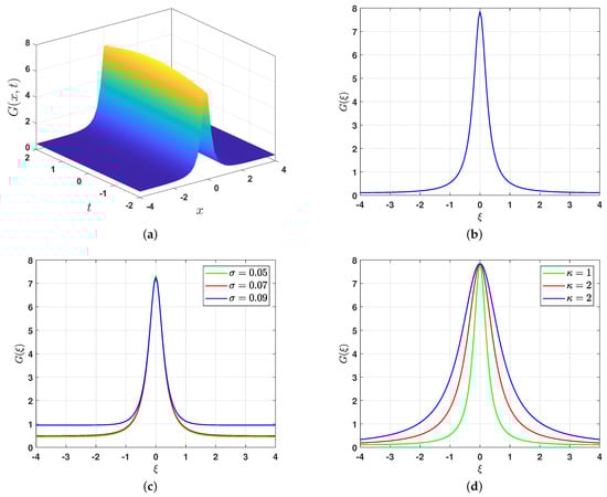
Figure 7.
Graphical representations of the solitary solution (21) and the influence of the wave velocity and wave number . (a) representation, (b) representation, (c) impact of , (d) impact of .
6. Quasi-Periodic Behavior
This section investigates the autoresonance behavior of a non-autonomous system in which the oscillator self-regulates under the influence of a variable periodic force. The perturbed version of the traveling wave system corresponding to Equation (2) emerges as a result of external effects. These effects are characterized by the inclusion of specific forces, represented as . It has the form
By substituting (3) into Equation (27), we derive a perturbed system that corresponds to the unperturbed system (7a,b) of the form
where is the Jacobi elliptic function [49]. The parameters are defined by (6), and the external periodic force is chosen as , where represents the strength of the external periodic force and denotes its frequency. This choice is significant because it can degenerate into trigonometric or hyperbolic functions as k approaches 0 or 1, respectively.
The unperturbed system (7a,b) is studied with the following parameter values: , , , , , , , and . These parameters are equivalent to , , and . We choose the initial conditions and , which results in , where q lies within the interval . This case corresponds to Case 8 in Table 1. Hence, the unperturbed system (7a,b) exhibits periodic behavior, as demonstrated in Figure 8a,b. Additionally, Figure 8c shows the plot of versus , which further confirms the system’s periodic behavior.
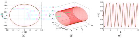
Figure 8.
The 2D, 3D, and time-series representations of the unperturbed system (7a,b) with the initial conditions and , where , , , , , , , and . (a) phase portrait, (b) phase portrait.
The inclusion of the free parameters , and , in addition to the three parameters , , and k associated with the perturbed term, adds complexity to understanding the periodic and chaotic dynamical behavior of the dual-mode Gardner model. This problem is addressed through the adoption of comprehensive and diverse strategies. This involves the presentation of 2D and 3D phase portraits, time series, and an examination of the influence of parameters through two distinct events. The investigation systematically varies the frequency (or strength) of the external force while keeping the other parameters fixed.
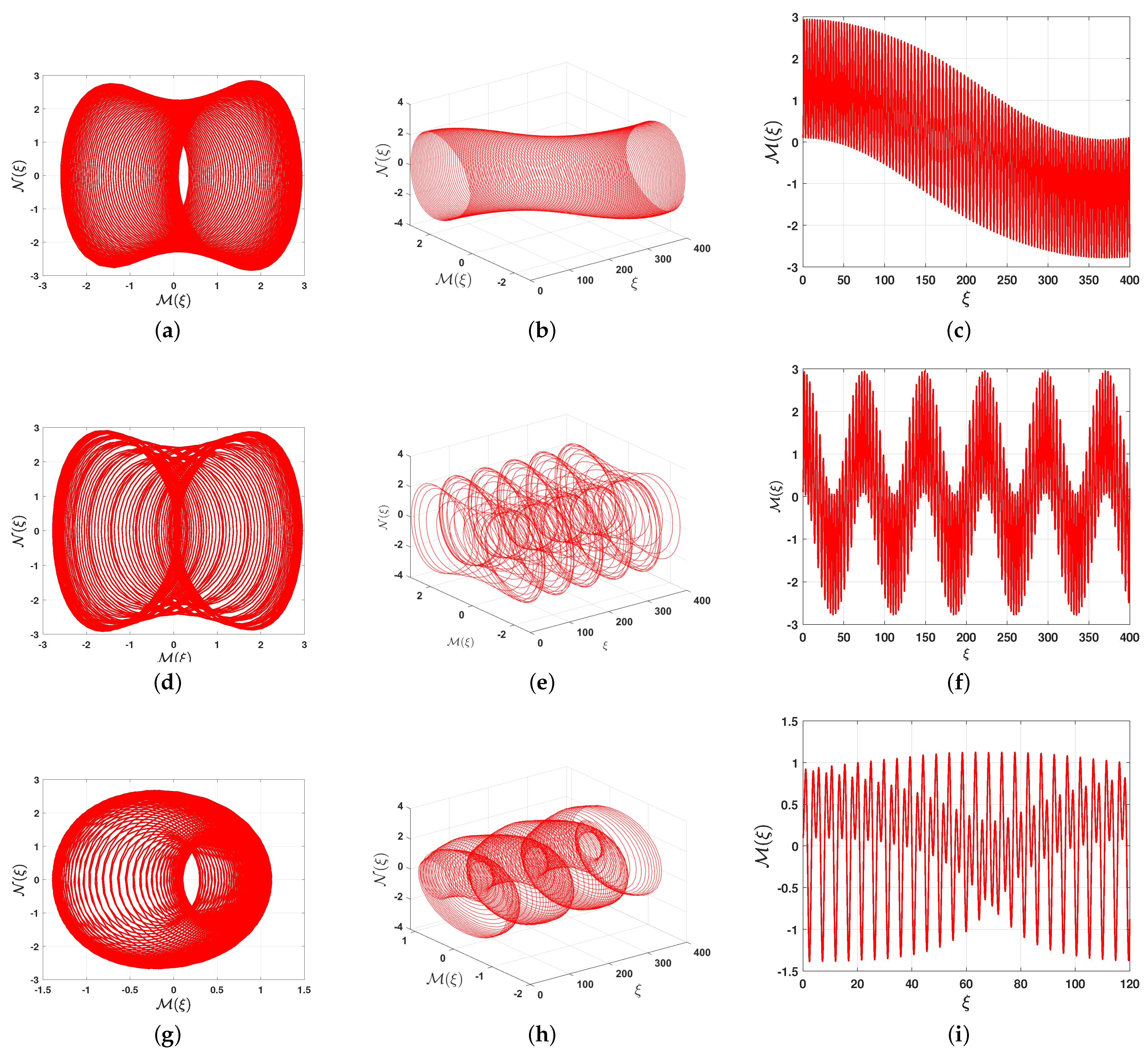
First, we assume the following parameter values: , , , , , , , , , and, consequently, , , and . In this section, we fix the strength of the external periodic effect at and allow the frequency to vary while keeping the initial condition fixed. For , Figure 9a and Figure 9b, which depict the and phase portraits of the perturbed system (28), show a quasi-periodic wave phenomenon, as confirmed by Figure 9c, which illustrates the solution as a function of . As the frequency increases to , the quasi-periodic behavior remains, as shown in Figure 9d–f. Moreover, chaotic behavior is absent even for , as confirmed by the and phase portraits in Figure 9g,h and the time-series representation depicted in Figure 9i. This is consistently observed due to the in commensurability of the frequency ratio.
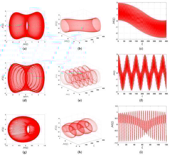
Figure 9.
The 2D, 3D, and time-series representations of the unperturbed system (28) with the initial condition , where , , , , , , , , , , and for different values of . (a) phase portrait, (b) phase portrait, (c) as a function of , (d) phase portrait, (e) phase portrait, (f) as a function of , (g) phase portrait, (h) phase portrait, (i) as a function of .
Second, we select suitable values for the physical parameters, fixing one of the parameters () while allowing all other parameters to vary. Specifically, we assume , , , , , , , , and . As a result, we have , , and . We present the 2D and 3D phase portraits, along with the time-series representation, for different values of the frequency and a fixed initial condition . For , the 2D and 3D phase portraits displayed in Figure 10a–c clearly show that the perturbed system (28) still exhibits quasi-periodic behavior. As the frequency increases to , the system dynamics shift to chaotic behavior, as shown in Figure 10d–f. Moreover, as the frequency further increases to , even more pronounced chaotic behavior is observed, as illustrated in Figure 10g–i.
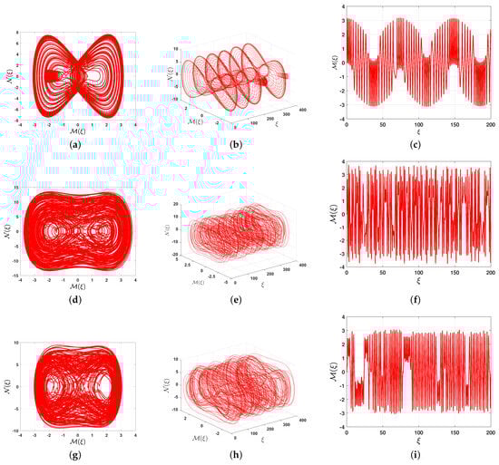
Figure 10.
The 2D, 3D, and time-series representations of the unperturbed system (28) with the initial condition , where , , , , , , , , and . (a) phase portrait, (b) phase portrait, (c) as a function of , (d) phase portrait, (e) phase portrait, (f) as a function of , (g) phase portrait, (h) phase portrait, (i) as a function of .
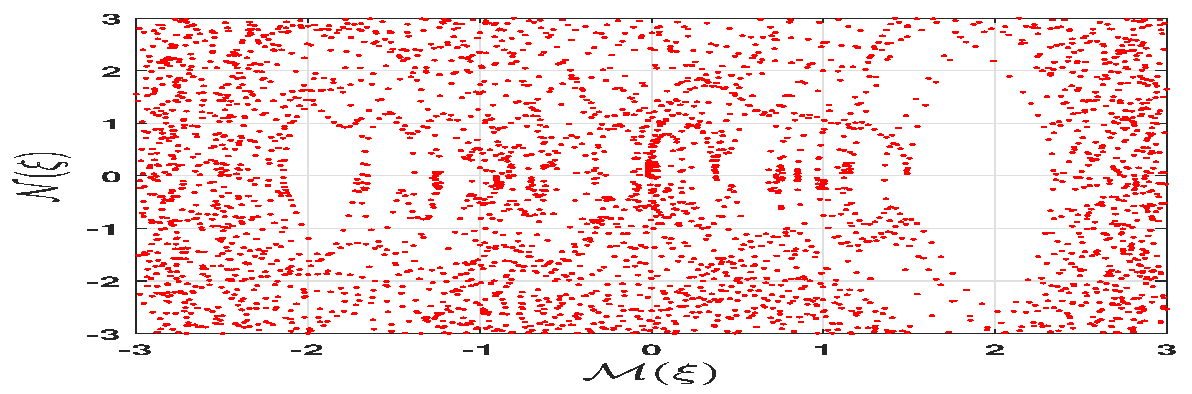
We introduce the Poincaré surface of section using the same parameter values as those in Figure 10, which lead to chaotic dynamics. The Poincaré surface of section shown in Figure 11 is irregular. In other words, it is dispersed and fails to form any recognizable pattern. This behavior arises because the perturbed dynamical system (28) exhibits chaotic dynamics.
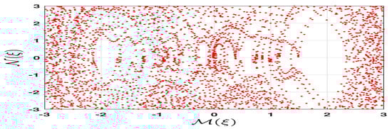
Figure 11.
Poincaré surface of section for the perturbed system (28) with the initial condition , where , , , , , , , , , and .
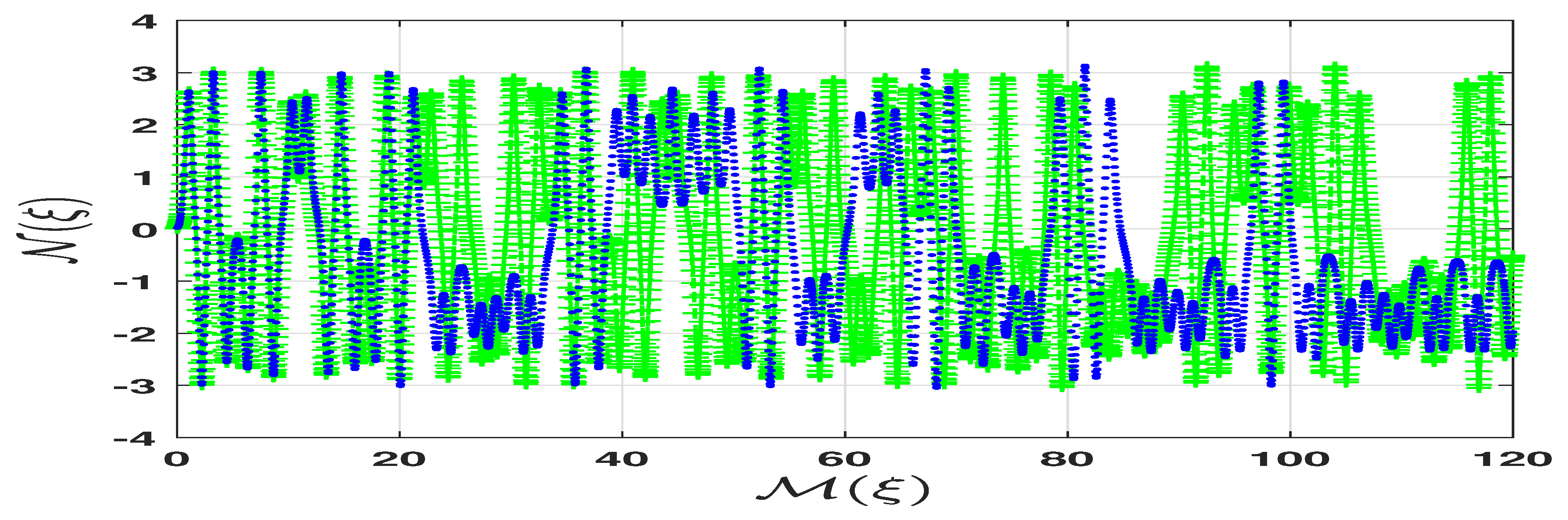
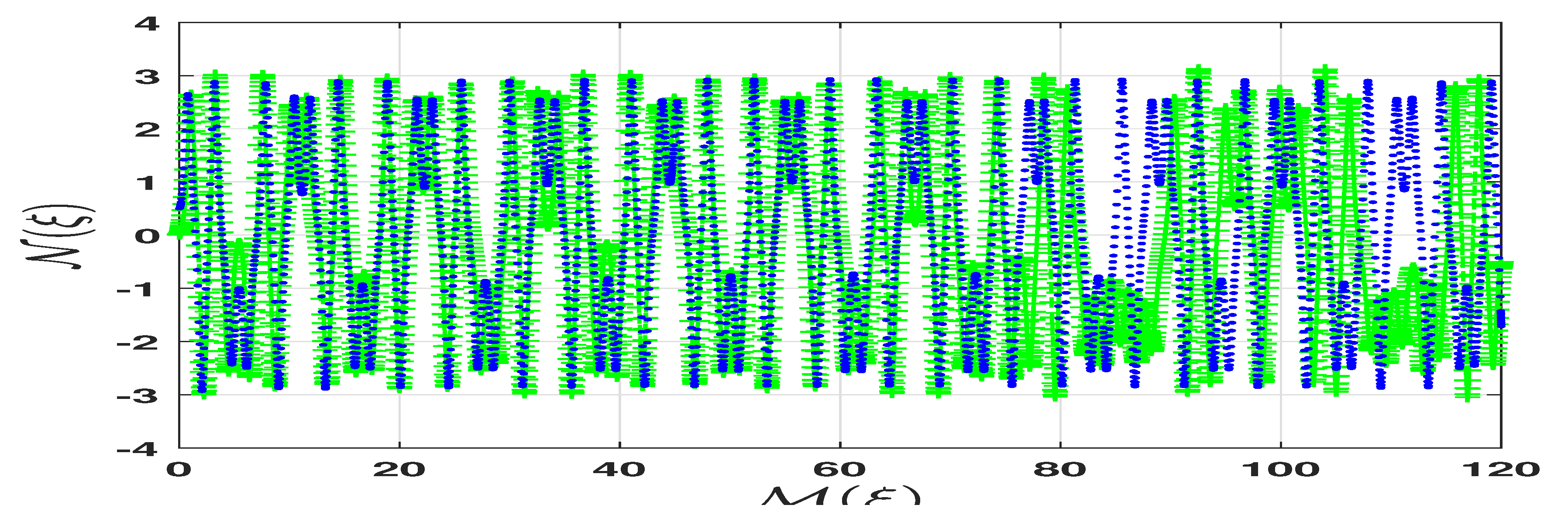
One can investigate the sensitivity of quasi-periodic waves by slightly altering the initial conditions. To explore this sensitivity, we consider two different initial conditions. The first set includes in green with a plus sign marker and in blue with a dot marker, as shown in Figure 12. The second set includes in green with a plus sign marker and in blue with a dot marker, as shown in Figure 13. Both figures compare the solutions of the system (28) for various initial conditions. The perturbed dynamical system (28) is sensitive to changes in the initial conditions due to its chaotic nature, which depends on the parameter values. Based on the observations and comparisons in Figure 12 and Figure 13, we conclude that the quasi-periodic chaotic behavior of the perturbed system is evident in its sensitivity to the initial conditions when specific parameter values are tested.

Figure 12.
Two-dimensional graph of sensitivity analysis of distinct initial conditions and in the perturbed system (28), where , , , , , , , , , and .
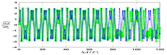
Figure 13.
Two-dimensional graph of sensitivity analysis of distinct initial conditions and in the perturbed system (28), where , , , , , , , , , and .
7. Conclusions
This study focuses on examining certain qualitative aspects of a dual-mode model for the Gardner equation derived from an ideal fluid. A wave transformation is applied to Equation (2), converting it into a dynamical system that corresponds to a Hamiltonian system with one degree of freedom. Consequently, finding a solution to Equation (2) is equivalent to solving the one- dimensional motion of a particle under the influence of a three-parameter potential function (9). This equivalence is significant as it allows for the determination of the real wave propagation intervals, which correspond to the possible real motions in Hamiltonian mechanics. Additionally, a bifurcation analysis is conducted on the traveling wave systems, highlighting its significance for several reasons, which are outlined below:
- (a)
- This approach enables us to classify the solutions before explicitly determining them by linking the solution types to the phase trajectories, as stated in Lemma 1. In other words, it provides the existence conditions for periodic, super-periodic, and solitary solutions, as shown in Table 1, Table 2, and Table 3, respectively.
- (b)
- This approach allows us to construct real (non-complex) solutions by considering the intervals of real wave propagation. Moreover, the significance of these intervals cannot be overlooked, as different intervals of real wave propagation yield different solutions. In other words, even under the same parameter conditions, distinct solutions arise due to variations in the intervals of real wave propagation.
- (c)
- This approach allows us to isolate unbounded solutions, which are less relevant in real-world applications. However, it is worth mentioning that these solutions can be computed using the same procedures as bounded solutions.
Although bifurcation analysis offers several advantages, as discussed earlier, it also has certain limitations in its application. For its effective use, the reduced traveling wave system must be conservative and Hamiltonian, with only one or two degrees of freedom. While this approach is theoretically applicable to Hamiltonian systems with higher degrees of freedom, practically implementing it in such cases remains highly challenging.
Taking into account the bifurcation conditions on the parameters, we construct new solutions to Equation (2), classifying them into periodic, super-periodic, and solitary solutions. These solutions are graphically illustrated through their and representations. Additionally, we analyze the influence of the wave number and wave velocity on some of these solutions, revealing their effects on amplitude and width variations. Finally, we introduce a periodic perturbation term to Equation (2), leading to the perturbed dynamical system (28). In the absence of this term, the unperturbed dynamical system (7a,b) is integrable, and consequently, it exhibits regular behavior. However, the inclusion of the perturbation alters the dynamical behavior, leading to quasi-periodic and chaotic dynamics. To analyze these effects, we present and phase diagrams, along with time-series representations. Furthermore, a sensitivity analysis is conducted for different initial conditions, and Poincaré maps are used to identify chaotic patterns in the model.
Now, let us compare the findings of this paper with those from the relevant literature. In [35], the authors utilized the tan/cot and tanh/coth methods to derive solutions, all of which were expressed in terms of tan, cot, tanh, and coth functions. In contrast, our solutions are constructed using Jacobi elliptic functions, rendering them entirely novel. Furthermore, in [42], the authors conducted a symmetry analysis and examined the conservation laws of model (2), as well as investigated its dynamical behavior under a cosine-perturbed term. Our work extends this perturbation to the Jacobi elliptic function , which reduces to the cosine-perturbed term when .
Funding
This work was supported by the Deanship of Scientific Research, Vice Presidency for Graduate Studies and Scientific Research, King Faisal University, Saudi Arabia [Grant no. KFU250790].
Data Availability Statement
No data were used to support this study.
Conflicts of Interest
The author declares that the research was conducted in the absence of any conflicts of interest.
References
- Gao, W.; Ismael, H.F.; Bulut, H.; Baskonus, H.M. Instability modulation for the (2 + 1)-dimension paraxial wave equation and its new optical soliton solutions in Kerr media. Phys. Scr. 2020, 95, 035207. [Google Scholar] [CrossRef]
- Fan, F.C.; Xu, Z.G.; Shi, S.Y. Soliton, breather, rogue wave and continuum limit for the spatial discrete Hirota equation by Darboux–Bäcklund transformation. Nonlinear Dyn. 2023, 111, 10393–10405. [Google Scholar] [CrossRef]
- Ablowitz, M.J.; Clarkson, P.A. Solitons, Nonlinear Evolution Equations and Inverse Scattering; Cambridge University Press: Cambridge, UK, 1991. [Google Scholar]
- Hirota, R. Exact N-soliton solutions of the wave equation of long waves in shallow-water and in nonlinear lattices. J. Math. Phys. 1973, 14, 810–814. [Google Scholar] [CrossRef]
- Alomair, A.; Al Naim, A.S.; Bekir, A. Exploration of Soliton Solutions to the Special Korteweg–De Vries Equation with a Stability Analysis and Modulation Instability. Mathematics 2024, 13, 54. [Google Scholar] [CrossRef]
- Matveev, V.B.; Salle, M.A. Darboux Transformations and Solitons; Springer Series in Nonlinear Dynamics; Springer: Berlin/Heidelberg, Germany, 1991. [Google Scholar]
- Konopelchenko, B.; Rogers, C. Bäcklund and reciprocal transformations: Gauge connections. Math. Sci. Eng. 1992, 185, 317–362. [Google Scholar]
- Rashedi, K.A.; Almusawa, M.Y.; Almusawa, H.; Alshammari, T.S.; Almarashi, A. Applications of Riccati–Bernoulli and Bäcklund Methods to the Kuralay-II System in Nonlinear Sciences. Mathematics 2024, 13, 84. [Google Scholar] [CrossRef]
- Dehghan, M.; Manafian, J. The solution of the variable coefficients fourth-order parabolic partial differential equations by the homotopy perturbation method. Z. Naturforsch. A 2009, 64, 420–430. [Google Scholar] [CrossRef]
- Fu, Z.; Liu, S.; Liu, S. New kinds of solutions to Gardner equation. Chaos Solitons Fractals 2004, 20, 301–309. [Google Scholar] [CrossRef]
- Li, X.; Wang, M. A sub-ODE method for finding exact solutions of a generalized KdV–mKdV equation with high-order nonlinear terms. Phys. Lett. A 2007, 361, 115–118. [Google Scholar] [CrossRef]
- Wang, M.; Li, X.; Zhang, J. Sub-ODE method and solitary wave solutions for higher order nonlinear Schrödinger equation. Phys. Lett. A 2007, 363, 96–101. [Google Scholar] [CrossRef]
- Wang, P.; Feng, X.; He, S. Lie Symmetry Analysis of Fractional Kersten–Krasil’shchik Coupled KdV–mKdV System. Qual. Theory Dyn. Syst. 2025, 24, 17. [Google Scholar] [CrossRef]
- Tanwar, D.V. On Lie symmetries, soliton interaction nature and conservation laws of Broer-Kaup-Kupershmidt system in shallow water of uniform depth. Phys. Scr. 2025, 100, 025225. [Google Scholar] [CrossRef]
- Gandarias, M.L.; Raza, N.; Umair, M.; Almalki, Y. Dynamical Visualization and Qualitative Analysis of the (4+ 1)-Dimensional KdV-CBS Equation Using Lie Symmetry Analysis. Mathematics 2024, 13, 89. [Google Scholar] [CrossRef]
- Moretlo, T.; Muatjetjeja, B.; Adem, A.R. Lie symmetry analysis and conservation laws of a two-wave mode equation for the integrable kadomtsev-petviashvili equation. J. Appl. Nonlinear Dyn. 2021, 10, 65–79. [Google Scholar] [CrossRef]
- Moretlo, T.; Muatjetjeja, B.; Adem, A. On the solutions of a (3+ 1)-dimensional novel kp-like equation. Iran. J. Sci. Technol. Trans. A Sci. 2021, 45, 1037–1041. [Google Scholar] [CrossRef]
- Mabenga, C.; Muatjetjeja, B.; Motsumi, T. Bright, dark, periodic soliton solutions and other analytical solutions of a time-dependent coefficient (2+ 1)-dimensional Zakharov–Kuznetsov equation. Opt. Quantum Electron. 2023, 55, 1117. [Google Scholar] [CrossRef]
- Elbrolosy, M.; Alhamud, M.; Elmandouh, A. Analytical solutions to the fractional stochastic (3+ 1) equation of fluids with gas bubbles using an extended auxiliary function method. Alex. Eng. J. 2024, 92, 254–266. [Google Scholar] [CrossRef]
- Pei, F.; Wu, G.; Guo, Y. Construction of infinite series exact solitary wave solution of the KPI equation via an auxiliary equation method. Mathematics 2023, 11, 1560. [Google Scholar] [CrossRef]
- Ryabov, P.N.; Sinelshchikov, D.I.; Kochanov, M.B. Application of the Kudryashov method for finding exact solutions of the high order nonlinear evolution equations. Appl. Math. Comput. 2011, 218, 3965–3972. [Google Scholar] [CrossRef]
- Elmandouh, A.; Elbrolosy, M. Integrability, variational principle, bifurcation, and new wave solutions for the Ivancevic option pricing model. J. Math. 2022, 2022, 9354856. [Google Scholar] [CrossRef]
- Elmandouh, A.; Aljuaidan, A.; Elbrolosy, M. The Integrability and Modification to an Auxiliary Function Method for Solving the Strain Wave Equation of a Flexible Rod with a Finite Deformation. Mathematics 2024, 12, 383. [Google Scholar] [CrossRef]
- Elbrolosy, M.; Elmandouh, A.; Elmandouh, A. Construction of new traveling wave solutions for the (2+ 1) dimensional extended Kadomtsev-Petviashvili equation. J. Appl. Anal. Comput 2022, 12, 533–550. [Google Scholar] [CrossRef]
- Elmandouh, A. Bifurcation, quasi-periodic, chaotic pattern, and soliton solutions for a time-fractional dynamical system of ion sound and Langmuir waves. Math. Methods Appl. Sci. 2025, 48, 3825–3841. [Google Scholar] [CrossRef]
- Elmandouh, A.; Fadhal, E. Bifurcation of exact solutions for the space-fractional stochastic modified Benjamin–Bona–Mahony equation. Fractal Fract. 2022, 6, 718. [Google Scholar] [CrossRef]
- El-Dessoky, M.M.; Elmandouh, A. Qualitative analysis and wave propagation for Konopelchenko-Dubrovsky equation. Alex. Eng. J. 2023, 67, 525–535. [Google Scholar] [CrossRef]
- Siddique, I.; Mehdi, K.B.; Jaradat, M.M.; Zafar, A.; Elbrolosy, M.E.; Elmandouh, A.A.; Sallah, M. Bifurcation of some new traveling wave solutions for the time–space M-fractional NEW equation via three altered methods. Results Phys. 2022, 41, 105896. [Google Scholar] [CrossRef]
- Zhang, X.Z.; Siddique, I.; Mehdi, K.B.; Elmandouh, A.; Inc, M. Novel exact solutions, bifurcation of nonlinear and supernonlinear traveling waves for M-fractional generalized reaction Duffing model and the density dependent M-fractional diffusion reaction equation. Results Phys. 2022, 37, 105485. [Google Scholar] [CrossRef]
- Burde, G.I.; Sergyeyev, A. Ordering of two small parameters in the shallow water wave problem. J. Phys. A Math. Theor. 2013, 46, 075501. [Google Scholar] [CrossRef]
- Karczewska, A.; Rozmej, P. Can simple KdV-type equations be derived for shallow water problem with bottom bathymetry? Commun. Nonlinear Sci. Numer. Simul. 2020, 82, 105073. [Google Scholar] [CrossRef]
- Karczewska, A.; Rozmej, P. (2+ 1)-dimensional KdV, fifth-order KdV, and Gardner equations derived from the ideal fluid model. Soliton, cnoidal and superposition solutions. Commun. Nonlinear Sci. Numer. Simul. 2023, 125, 107317. [Google Scholar] [CrossRef]
- Rozmej, P.; Karczewska, A. Soliton, periodic and superposition solutions to nonlocal (2+ 1)-dimensional, extended KdV equation derived from the ideal fluid model. Nonlinear Dyn. 2023, 111, 18373–18389. [Google Scholar] [CrossRef]
- Korsunsky, S.V. Soliton solutions for a second-order KdV equation. Phys. Lett. A 1994, 185, 174–176. [Google Scholar] [CrossRef]
- Sadiq, S.; Javid, A.; Riaz, M.B.; Basendwah, G.A.; Raza, N. Bi-directional solitons of dual-mode Gardner equation derived from ideal fluid model. Results Phys. 2024, 57, 107337. [Google Scholar] [CrossRef]
- Gardner, C.S. Korteweg-de Vries equation and generalizations. IV. The Korteweg-de Vries equation as a Hamiltonian system. J. Math. Phys. 1971, 12, 1548–1551. [Google Scholar] [CrossRef]
- Tribeche, M.; Amour, R.; Shukla, P. Ion acoustic solitary waves in a plasma with nonthermal electrons featuring Tsallis distribution. Phys. Rev. E—Stat. Nonlinear Soft Matter Phys. 2012, 85, 037401. [Google Scholar] [CrossRef]
- Wazwaz, A.M. Two-mode fifth-order KdV equations: Necessary conditions for multiple-soliton solutions to exist. Nonlinear Dyn. 2017, 87, 1685–1691. [Google Scholar] [CrossRef]
- Jaradat, H.; Alquran, M.; Syam, M.I. A reliable study of new nonlinear equation: Two-mode Kuramoto–Sivashinsky. Int. J. Appl. Comput. Math. 2018, 4, 1–8. [Google Scholar] [CrossRef]
- Ambrose, D.M.; Mazzucato, A.L. Global solutions of the two-dimensional Kuramoto–Sivashinsky equation with a linearly growing mode in each direction. J. Nonlinear Sci. 2021, 31, 1–26. [Google Scholar] [CrossRef]
- Wazwaz, A.M. Two-mode Sharma-Tasso-Olver equation and two-mode fourth-order Burgers equation: Multiple kink solutions. Alex. Eng. J. 2018, 57, 1971–1976. [Google Scholar] [CrossRef]
- Jhangeer, A.; Beenish; Říha, L. Symmetry analysis, dynamical behavior, and conservation laws of the dual-mode nonlinear fluid model. Ain Shams Eng. J. 2025, 16, 103178. [Google Scholar] [CrossRef]
- Goldstein, H. Classical Mechanics Addison-Wesley Series in Physics; Addison-Wesley: Reading, MA, USA, 1980. [Google Scholar]
- Gantmacher, F. Lectures in Analytical Mechanics; Mir: Moscow, Russia, 1970. [Google Scholar]
- Meng, Q.; He, B.; Long, Y.; Rui, W. Bifurcations of travelling wave solutions for a general Sine–Gordon equation. Chaos Solitons Fractals 2006, 29, 483–489. [Google Scholar] [CrossRef]
- He, B.; Li, J.; Long, Y.; Rui, W. Bifurcations of travelling wave solutions for a variant of Camassa–Holm equation. Nonlinear Anal. Real World Appl. 2008, 9, 222–232. [Google Scholar]
- Dubinov, A.E.; Kolotkov, D.Y.; Sazonkin, M.A. Supernonlinear waves in plasma. Plasma Phys. Rep. 2012, 38, 833–844. [Google Scholar] [CrossRef]
- Saha, A.; Banerjee, S. Dynamical Systems and Nonlinear Waves in Plasmas; CRC Press: Boca Raton, FL, USA, 2021; p. x+207. [Google Scholar]
- Byrd, P.F.; Friedman, M.D. Handbook of Elliptic Integrals for Engineers and Scientists, 2nd ed.; Die Grundlehren der Mathematischen Wissenschaften, Band 67; Springer: New York, NY, USA; Berlin/Heidelberg, Germany, 1971; p. xvi+358. [Google Scholar]
- Saha, A.; Tamang, J. Effect of q-nonextensive hot electrons on bifurcations of nonlinear and supernonlinear ion-acoustic periodic waves. Adv. Space Res. 2019, 63, 1596–1606. [Google Scholar] [CrossRef]
- Tamang, J.; Saha, A. Dynamical behavior of supernonlinear positron-acoustic periodic waves and chaos in nonextensive electron-positron-ion plasmas. Z. Naturforsch. A 2019, 74, 499–511. [Google Scholar] [CrossRef]

Disclaimer/Publisher’s Note: The statements, opinions and data contained in all publications are solely those of the individual author(s) and contributor(s) and not of MDPI and/or the editor(s). MDPI and/or the editor(s) disclaim responsibility for any injury to people or property resulting from any ideas, methods, instructions or products referred to in the content. |
© 2025 by the author. Licensee MDPI, Basel, Switzerland. This article is an open access article distributed under the terms and conditions of the Creative Commons Attribution (CC BY) license (https://creativecommons.org/licenses/by/4.0/).